Early dark energy and its interaction with dark matter

Abstract

We study a class of early dark energy models which has substantial amount of dark energy in the early epoch of the universe. We examine the impact of the early dark energy fluctuations on the growth of structure and the CMB power spectrum in the linear approximation. Furthermore we investigate the influence of the interaction between the early dark energy and the dark matter and its effect on the structure growth and CMB. We finally constrain the early dark energy model parameters and the coupling between dark sectors by confronting to different observations.

I Introduction

From astronomical observations, it is convincing that our universe is undergoing accelerated expansion. The driving force of this acceleration is dark energy(DE), which composes roughly $70\%$ of the total energy budget of our universe. The physical nature of DE, together with its origin and time evolution, is one of the most enigmatic puzzles in modern cosmology. The simplest explanation of DE is the cosmological constant with equation of state (EoS) $w=-1$. Although the cosmological constant fits well to current observational data, it suffers serious theoretical problems. One is the cosmological constant problem, the fact that the quantum field theory prediction for the value of $\Lambda$ is about hundred orders of magnitude larger than the observation coincidence . Another problem, more closely related to the cosmological evolution itself, is the coincidence problem, namely why being a constant, the $\Lambda$ value becomes important for the evolution of the universe just at the present moment coin . Besides the cosmological constant, there are other alternative explanations of DE. But so far, the focus has been on the EoS of DE and in particular on its current value $w_{0}$.

It is rather the amount of DE, $\Omega_{de}$, than the EoS, that influences the evolution of our universe. In this spirit, an interesting sub-class of DE models involving a non-negligible DE contribution at early times has been proposed. These models are called Early Dark Energy (EDE), and have been extensively studied recently. EDE models can potentially alleviate the coincidence problem. Furthermore, they can influence the cosmic microwave background 1304.3724 ; Doran2001 ; 1003.1259 ; astro-ph/0508132 ; astro-ph/0611507 ; 1305.2209 ; 0901.0605 , big-bang nucleosynthesisMuller and large-scale structure formation Bartelmann ; 1004.0437 ; 1207.1723 ; 0809.3404 ; 1303.0414 ; xx ; Baldi . For now, it would be fair to say that there are no strong observational constraints on the EDE models, and it is especially difficult to discriminate EDE models which have $w=-1$ at present from the $\Lambda$CDM model.

In this paper, we will focus on a specific EDE model, which is similar to that originally introduced by Wetterich wetterich and further examined in 0809.3404 . This model is characterized by a low but non-vanishing DE density at early times with the EoS varying with time in the form

$$w(z)=\frac{w_{0}}{1+b\ln{(1+z)}^{2}},\hskip 28.45274ptb=-\frac{3w_{0}}{\ln{(\frac{1-\Omega_{de,e}}{\Omega_{de,e}})}+\ln{(\frac{1-\Omega_{m,0}}{\Omega_{m,0}})}}$$ (1)

where $w_{0}$ and $\Omega_{de,0}=1-\Omega_{m,0}$ represent the present-day EoS and amount of DE, respectively, while $\Omega_{de,e}$ gives the average energy density parameter at early times. The EDE model described in (1) has been confronted to the type Ia supernova test including samples at $z>1.25$ Rahvar yungui . The impact of this EDE cosmology on galaxy properties has been studied by coupling high-resolution numerical simulations with semi-analytic modeling of galaxy formation and evolution 1207.1723 . The available results highlight that such EDE model leads to important modifications in the galaxy properties with respect to a standard $\Lambda$CDM universe.

We use this dynamical EDE parametrization to further discuss the influence of this specific model on the cosmic microwave background radiation (CMB) and compare with the $\Lambda$CDM prediction. For dynamical DE models, in contrast with $\Lambda$CDM, they possess DE fluctuations. In the linear regime, these fluctuations for usual DE models, for example quintessence, are usually several orders of magnitude smaller than that of dark matter (DM), so that DE fluctuations are usually neglected in studies of CMB and structure formations in the linear approximation. It would be interesting to examine the presence of the EDE fluctuation and its impact on the DM perturbations and CMB, and compare with the usual assumption of nearly homogeneous EDE and $\Lambda$CDM models. This can help to distinguish between homogeneous and inhomogeneous EDE models and also disclose the difference from the $\Lambda$CDM model. Moreover we will attempt to constrain this EDE model using current data. In 0901.0605 one different type of EDE model was constrained by using observational data at high redshift including the WMAP five year data for CMB, but in their study they have not compared different effects brought by the inhomogeneous and homogeneous EDE.

It is clear that DM and DE are two main components of our universe, which compose almost $95\%$ of the total universe. It is a special assumption that these two biggest components existing independently in the universe. A more natural understanding, in the framework of field theory, is to consider that there is some kind of interaction between them. It has been shown that the interaction between DM and DE is allowed by astronomical observations and can help to alleviate the coincidence problem, see for example 1311.7380 ; 1308.1475 ; 1012.3904 ; 1001.0097 ; 0710.1198 and references therein. It would be of great interest to extend the previous studies to the interaction between EDE and DM. With the non-negligible DE energy density at high redshift, the interaction between dark sectors will start to play the role earlier. To investigate the influence of the interaction between EDE and DM on the structure growth and CMB signals is the second objective of this paper.

The outline of the paper is the following. In the next section, we will first present the background evolution of the EDE model and discuss the influence of the interaction between dark sectors on the background dynamics. And then we will study evolutions of linear perturbations of a system with EDE and pressureless matter and calculate the growth of structure. We will examine the effect of the interaction between EDE and DM on the linear perturbations. Section III is devoted to the study of the CMB power spectrum. In Section IV we will present the constraint of the EDE model from fittings to current observational data and in the last section we will present our conclusions.

II Analytical Formalism

In this paper, we investigate the EDE model presented in (1), in which there is a low but non-vanishing DE density at early times. We modified CAMB code to examine the influences of the EDE on the background evolution, linear perturbation and CMB power spectrum by performing analysis for two models ‘EDE1’ and ‘EDE2’, which have $w_{0}=-0.93,\Omega_{de,e}=2\times 10^{-4}(b=0.29,\Omega_{m,0}=0.25)$ and $w_{0}=-1.07,\Omega_{de,e}=2\times 10^{-4}(b=0.33,\Omega_{m,0}=0.25)$, respectively.

Figure 1 shows the evolutions of EoS in EDE models that we examine in this work. The amount of DE at early times is non vanishing and EDE models approach to the cosmological constant scenario at recent times. The EDE1 model has EoS always above $-1$, while EDE2 EoS can cross $-1$ and stay below $-1$ at present.

Figure 1: EoS of two EDE models. The dotted line refers to the EDE1 with b=0.01.

In the spatially flat Friedmann-Robertson-Walker(FRW) universe, the evolutions of the energy densities of DE and DM in the background spacetime are governed by

$$\rho^{\prime}_{dm}+3\mathcal{H}\rho_{dm}=aQ_{dm}$$

$$\rho^{\prime}_{de}+3\mathcal{H}(1+w)\rho_{de}=aQ_{de},$$ (2)

where $H$ is the Hubble constant and $\mathcal{H}=aH$ with $a$ the scale factor of the universe. $Q_{\alpha}$ indicates the interaction between dark sectors, where the subscript ‘$\alpha$’ refers to ‘$dm$’ or ‘$de$’ respectively. We show the evolution of the DE fractional energy density when there is no interaction between DE and DM in Figure 2. In the left panel of Figure 2, we compare the $\Omega_{de}$ for EDE1 with constant EoS DE and cosmological constant. We can see that for the model EDE1, DE started to have a significant ratio in the budget of the universe earlier, which help to alleviate the coincidence problem. We also compare the evolution of $\Omega_{de}$ for different EDE models with that of the cosmological constant in the right panel of Figure 2. The evolution of $\Omega_{de}$ shows that the model EDE1 is favorable to ease the coincidence problem. To see more clearly, we present the behavior on the ratio $\rho_{dm}/\rho_{de}$ in Figure 3. It is easy to see that the ratio for EDE1 is smaller at early times. This shows that the ratio for EDE1 evolves slower, so that it has longer period for the energy densities of EDE1 and DM to be comparable, in the spirit of alleviating the coincidence problem.

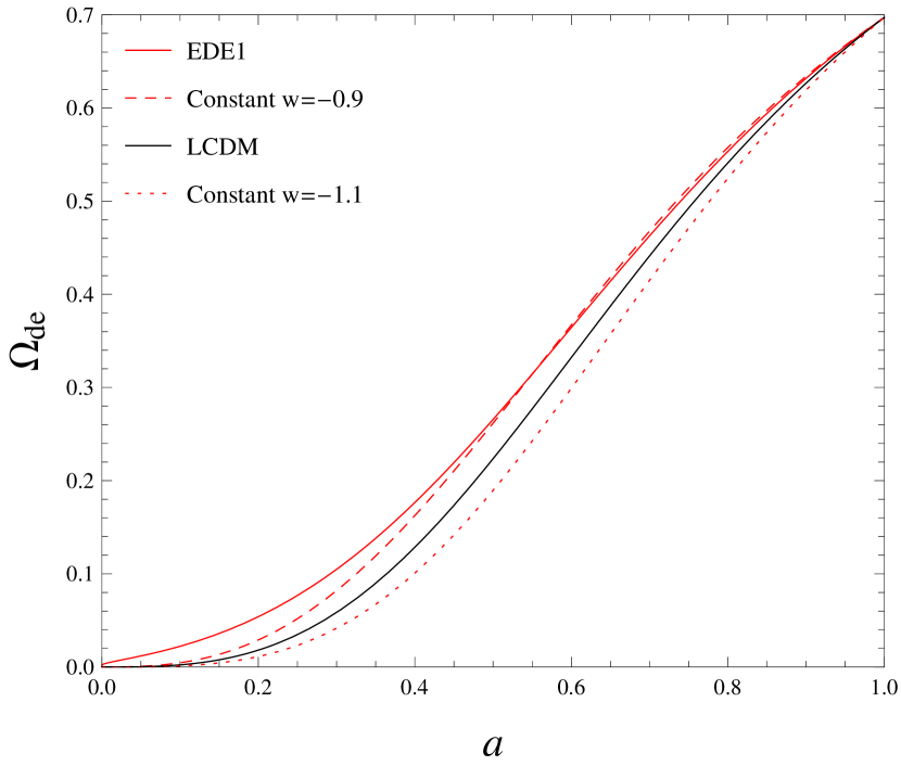
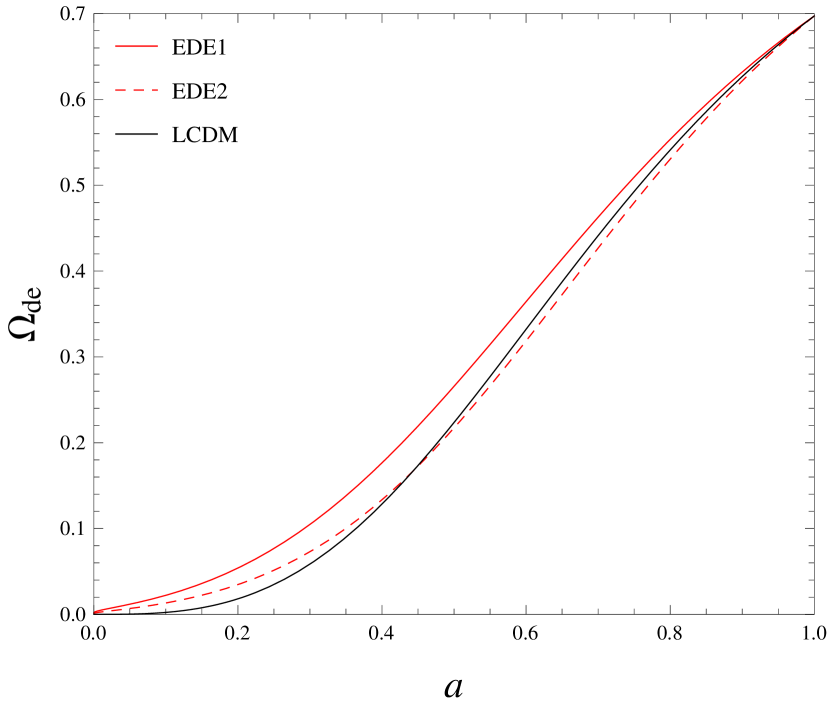
Figure 2: The evolutions of DE fractional energy densities for different DE models when there is no interaction between dark sectors.

Figure 3: The ratio of DM densities to DE densities for different DE models when there is no interaction between dark sectors.

Since we know the nature of neither DM nor DE, it is hard to describe the interaction between them, although there are some attempts on this task 1202.0499 ; Sandro1 ; Sandro2 ; 1206.2589 . Our study on the interaction between dark sectors will concentrate on the phenomenological descriptions. We assume there is energy flow due to the interaction between dark sectors where the coupling vector is defined in the form $Q^{\nu}=(\frac{Q}{a},0,0,0)^{T}$ 1012.3904 , and $Q$ takes the phenomenological form $Q=3\lambda_{1}H\rho_{dm}$ or $Q=3\lambda_{2}H\rho_{de}$, where $\lambda_{1}$ and $\lambda_{2}$ refer to the strength of the respective couplings.

We plot the evolution of the DE fractional energy density in Figure 4. In the left panel, we choose the interaction as being proportional to the energy density of DM. For the EDE model, with the positive coupling proportional to the DM energy density ($\lambda_{1}>0$), the influence of DE in the universe evolution appeared much earlier. The positive coupling, in our notation, indicates that energy flows from DE to DM 1311.7380 ; 1308.1475 ; 1012.3904 ; 1001.0097 ; 0710.1198 . For the same amount of DE today, with the positive coupling, it implies that DE density was higher in the past. The coupling strength $\lambda_{1}$ cannot be chosen negative, since the negative $\lambda_{1}$ will lead to the negative DE fractional energy density $\Omega_{de}$ at early time of the universe, as is shown in the middle panel of Figure 4, which is certainly unphysical. In the right panel of Figure 4, we show the case where the interaction is proportional to the DE density. We see that for the EDE1 model with positive coupling ($\lambda_{2}>0$), there was more EDE at high redshift if the present DE amount is the same as that of the $\Lambda$CDM model, what we also argued to have consequences related to DM phenomenology in accordance to results of BOSS abdferreirawang . But comparing with the left panel, the influence of the coupling is weaker in the right panel. This is easy to understand, because in the right panel the interaction is proportional to DE energy density, which was much lower than that of DM at early times in the universe.

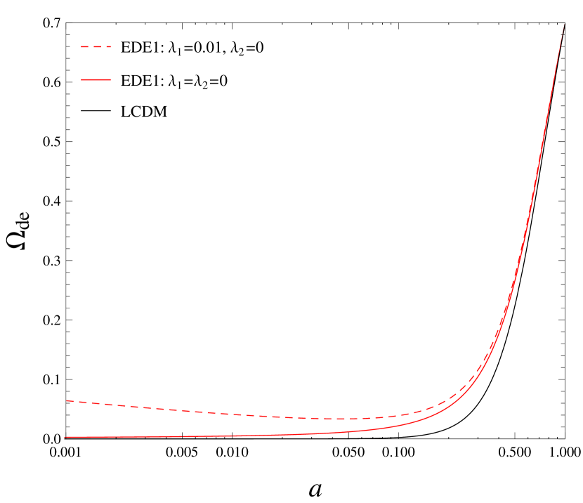
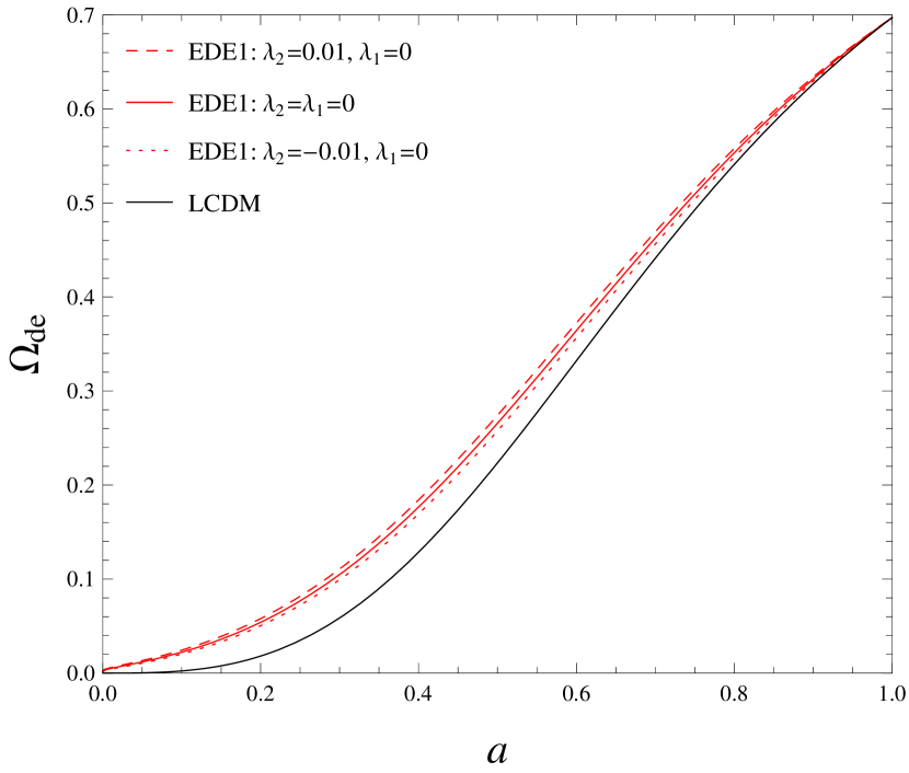
Figure 4: The evolutions of DE fractional densities when there is interaction between dark sectors.

Besides the background dynamics, we can extend the study to the linear relativistic evolution of the system of DE and DM. The gauge invariant linear perturbation equations of the system were derived in0807.3471 ; 0902.0660 ; 0906.0677 ; 1012.3904 . Using the phenomenological form of the energy transfer between dark sectors defined above, the equations yield

$$D_{dm}^{\prime} = -kU_{dm}+3\mathcal{H}\Psi{(\lambda_{1}+\lambda_{2}/r)}-3(\lambda_{1}+\lambda_{2}/r)\Phi^{\prime}+3\mathcal{H}\lambda_{2}(D_{de}-D_{dm})/r,$$

$$U_{dm}^{\prime} = -\mathcal{H}U_{dm}+k\Psi-3\mathcal{H}(\lambda_{1}+\lambda_{2}/r){U_{dm}};$$

$$D_{de}^{\prime} = -3\mathcal{H}(C_{e}^{2}-w)D_{de}+\{3w^{\prime}-9\mathcal{H}(w-C_{e}^{2})(\lambda_{1}{r}+\lambda_{2}+1+w)\}\Phi,$$

$$- 9\mathcal{H}^{2}(C_{e}^{2}-C_{a}^{2})\frac{U_{de}}{k}+3(\lambda_{1}{r}+\lambda_{2})\Phi^{\prime}-3\Psi\mathcal{H}(\lambda_{1}{r}+\lambda_{2})+3\mathcal{H}\lambda_{1}{r}(D_{de}-D_{dm})$$

$$- 9\mathcal{H}^{2}(C_{e}^{2}-C_{a}^{2})(\lambda_{1}{r}+\lambda_{2})\frac{U_{de}}{(1+w)k}-kU_{de},$$

$$U_{de}^{\prime} = -\mathcal{H}(1-3w)U_{de}-3kC_{e}^{2}(\lambda_{1}{r}+\lambda_{2}+1+w)\Phi+3\mathcal{H}(C_{e}^{2}-C_{a}^{2})(\lambda_{1}{r}+\lambda_{2})\frac{U_{de}}{(1+w)}$$ (3)

$$+ 3(C_{e}^{2}-C_{a}^{2})\mathcal{H}U_{de}+kC_{e}^{2}D_{de}+(1+w)k\Psi+3\mathcal{H}(\lambda_{1}{r}+\lambda_{2})U_{de}\quad,$$

where $\Psi,\Phi$ are gauge invariant gravitational potentials, $D_{\alpha}=\delta_{\alpha}-\frac{\rho^{\prime}_{\alpha}}{\rho\mathcal{H}}\Phi$ is the gauge invariant density contrast, $U_{\alpha}=(1+w_{\alpha})V_{\alpha}$, $V_{\alpha}$ is the gauge invariant peculiar velocity, and $r\equiv\rho_{dm}/\rho_{de}$ is the energy density ratio of DM and DE. $C_{a}$ is the adiabatic sound speed of DE and $C_{e}$ is the effective sound speed of DE which we will set to be $1$ in this work. Having these perturbation equations, we are in a position to discuss the evolutions of DE and DM density perturbations.

Assuming $\lambda_{1}=\lambda_{2}=0$ in (3), we display the evolution of the DE perturbation in the left panel of Figure 5. In contrast to the DE models with constant EoS, which always have very small DE fluctuations, we see that although the fluctuation of EDE decays to zero as its EoS approaches to the cosmological constant, at early times, when EDE started to play a significant role, its fluctuation was not too small. It would be interesting to investigate how the EDE perturbation influences the growth of DM perturbations. We display the result in Figure 6, where we show the evolution of DM density perturbation in different DE models. It is clear that the earlier presence of non-negligible DE fractional density in the background suppresses the growth in the DM perturbation. To see more closely, we have compared the evolution of the DM perturbation to the standard $\Lambda$CDM model in Figure 6. DM perturbations were suppressed compared with $\Lambda$CDM model if DE is described by EDE2, constant $w=-0.9$ and EDE1. The only exception is when DE has a constant EoS $w=-1.1$. The difference in the structure growth from that of the $\Lambda$CDM model can be mainly attributed to the differences in the background DE fractional energy density from the standard $\Lambda$CDM model. The suppression of the growth of perturbations was caused by the excessive amount of DE than that in the $\Lambda$CDM model at early epoch, which hindered gravitational attraction and weakened the growth of DM perturbations. For the EDE models, especially EDE1, the further excess of $\Omega_{de}$ at early times suppresses the structure growth even more. The solid lines indicate the models having DE perturbation, while the dashed lines are for the homogeneous DE models where the DE perturbations are neglected. For the DE models with constant EoS, the difference of effects on the DM perturbations caused by homogeneous and inhomogeneous DE are negligible. This can be further seen in Figure 6. But for EDE models, we clearly see the differences between the solid and dashed lines for the inhomogeneous and homogeneous DE. Figure 6 shows this property much clearer. This is understandable because for the DE with constant EoS, the DE perturbation itself is tiny. However for the EDE models, we clearly see that different from the homogeneous DE model, the DE perturbations do have impact on DM perturbations.

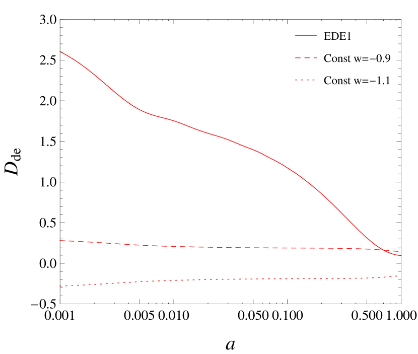
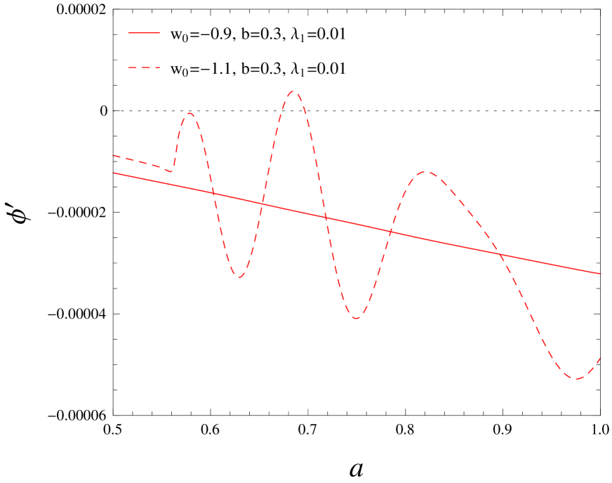
Figure 5: The left panel: The evolutions of DE perturbations. The right panel: The time derivative of the gravitational potential.

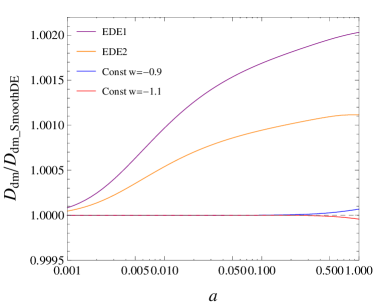
Figure 6: (a) The evolutions of DM perturbations. (b) The comparison of DM perturbation evolutions with that of $\Lambda$CDM model. (c) The comparison of DM perturbation evolutions with and without DE perturbations. The solid lines refer to models taking into account DE perturbations. The dashed lines refer to the models assuming homogenous DE.

Considering the interaction between dark sectors, the situation becomes more complicated. To see clearly the influence of the interaction in dark sectors on the linear perturbations, we concentrate on the DE model EDE1, because in EDE1 the DE EoS is always greater than $-1$. $1+w$ has to be positive in order to avoid oscillation in the time derivative of the gravitational potential on large scales if the interaction between dark sectors is proportional to the energy density of DM, which is inconsistent with observations, as shown in the right panel of Figure 5. In Figure 7, we see that at the present moment for the model with energy decay from EDE to DM, the DM perturbation is smaller, which is different from the case with energy decay in the opposite direction. This is easy to understand, because for the positive coupling the background $\Omega_{de}$ was bigger in the past, which hindered the structure growth. In Figure 7, we present the comparison of the DM perturbations between the interacting EDE model and the $\Lambda$CDM model. It is clear that, comparing with $\Lambda$CDM model, EDE interacting with DM leads to smaller DM perturbations. For the interaction between dark sectors proportional to the energy density of DM, the effect of interaction showed up earlier. A positive $\lambda_{1}$ implies more DE in the past, bringing further suppression in the DM perturbations at early time. For the interaction between dark sectors proportional to the density of DE, the effect showed up later when DE started to dominate. A positive $\lambda_{2}$ indicates the energy flow from EDE to DM, which implies that there was more DE in the past, preventing the DM perturbations further. This explains why the line in Figure 7 with positive $\lambda_{2}$ is lower. For negative $\lambda_{2}$, energy flows from DM to DE. To have the observed amount of DM now, there must be more DM in the past, which implies faster growth of DM perturbation. Since this effect of interaction started to appear when DE became important and became more influential in the era of accelerated expansion, lines corresponding to positive and negative $\lambda_{2}$ in Figure 7 deviate from the non-interacting case late in the history of the universe. The solid and dashed lines in Figure 7 refer to inhomogeneous and homogeneous DE, respectively. We see that DM perturbations differ by including the DE perturbations or not. This can be seen much clearer in Figure 7. Comparing with Fig.6, we see that when energy flows from DE to DM, the difference in the DM perturbations caused by the inhomogeneous DE and homogeneous DE is enlarged. Also from Figure 7 we see that the difference in the DM perturbations between inhomogeneous and homogeneous DE is more sensitive to the coupling if it is proportional to the energy density of DM.

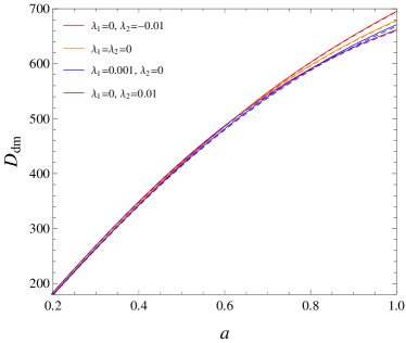
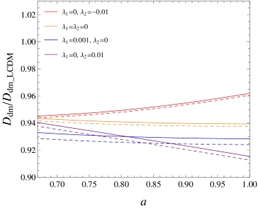
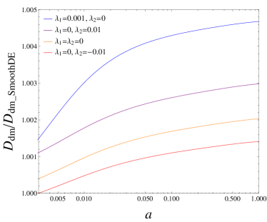
Figure 7: (a) DM perturbations when EDE interacts with DM. (b) The comparison of DM perturbation evolutions with that of $\Lambda$CDM model. (c) The comparison of DM perturbation evolutions between models with and without DE perturbations. The solid lines refer to models taking into account DE perturbations. The dashed lines refer to the models assuming homogenous DE.

III CMB power spectrum

Once we have the understanding of the linear perturbations for DM and DE, we can proceed to study the effects of DE models on CMB. On large scales, the CMB power spectrum is composed of the ordinary Sachs-Wolfe (SW) effect and the Integrated SW (ISW) effect. The SW effect indicates the photons’ initial condition when it left the last scattering surface while the ISW effect is the contribution due to the change of the gravitational potential when photons passing through the universe on their way to earth. The gauge invariant gravitational potential in the absence of anisotropic stress can be given by the Poisson equation $k^{2}\Phi=-4\pi Ga^{2}\delta\rho$. Its derivative in DM plus DE universe, which is the source term for the ISW contribution, is given by $k^{2}\Phi^{\prime}=-4\pi G\frac{\partial}{\partial\eta}[a^{2}(\delta\rho_{dm}+\delta\rho_{de})]$. Thus the large scale CMB power spectrum depends on the evolution of the density perturbations of DE and DM. However it should be noted that ISW effect is complicated. Besides density perturbations in DM and DE, other cosmological parameters such as the EoS of DE, background energy densities and $H_{0}$ etc. also have influence on it. Only for the same background evolution, the large scale CMB power spectrum can be interpreted in terms of the evolution of the density perturbations for DE and DM.

Neglecting the interaction between dark sectors, for DE with constant EoS $w=-0.9$, we show the CMB power spectrum in Figure 8. Comparing with the $\Lambda$CDM model, there is little difference in CMB at small $l$ ISW effect. The ISW effect relates to the time variation of the gravitational potentials, which demonstrates little difference between DE with constant EoS and $\Lambda$CDM xx . For DE with constant EoS, the CMB power spectrum keeps the same no matter we include the DE fluctuations in the computation or not. The DE fluctuations do not show up in the CMB power spectrum. This is because for DE with constant EoS, the DE perturbation is negligible. And the result at large scale CMB power spectrum agrees with what disclosed in the growth of DM perturbation in the previous section where the DE fluctuations do not show up for the DE with constant EoS. Thus including the DE fluctuations, the CMB power spectrum remains the same as when the perturbations to DE is not taken into account.

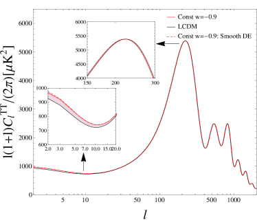
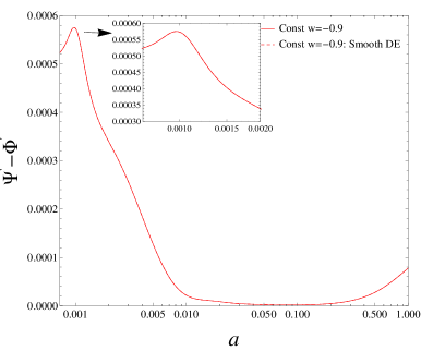
Figure 8: CMB power spectrum and the time derivative of the gravitational potential when DE EoS is constant, $w=-0.9$

For the EDE models, we observed some interesting results in CMB. We considered both cases where EDE is homogeneous and inhomogeneous in Figures 9. Besides a slight shift of the position of the acoustic peaks with respect to $\Lambda$CDM model, we see that the CMB power spectrum at small $l$ is different between inhomogeneous and homogeneous EDE. In homogeneous EDE model in which DE fluctuations is neglected, the small $l$ spectrum is suppressed as compared with that of $\Lambda$CDM. In inhomogeneous EDE model in which DE fluctuations is taken into account, we observe an enhanced power spectrum at low $l$ with respect to $\Lambda$CDM. For a given EDE model, the evolutions of background cosmological parameters are the same, the differences in the large scale CMB power spectrum can be attributed to the evolutions of DE and DM density perturbations. In the last section, we learnt that the inhomogeneity in EDE will have an impact on the DM perturbations. For the inhomogeneous EDE, the DM perturbation is stronger. The inhomogeneous EDE perturbation also evolves with time. These effects result in a change of the gravitational potential and the varition of the gravitational potential in time leads to the differences in the ISW effect in CMB.

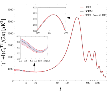
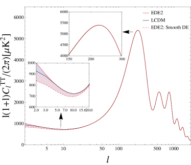
Figure 9: CMB power spectrum for EDE models. We compare the CMB power spectrum for the universe with inhomogeneous DE and homogeneous DE. For EDE models, the solid lines refer to inhomogeneous DE and the dashed lines refer to homogeneous DE.

Including interaction between dark sectors, we have a richer physics in CMB. In the left panel of Figure 10, we present the CMB power spectrum for the interaction proportional to the energy density of DM. With a positive interaction, we see that the difference at low $l$ CMB between homogeneous and inhomogeneous EDE is enlarged compared with the zero coupling case. This can be attributed to the enlarged differences in the EDE perturbations together with the DM perturbations between including the EDE fluctuations or not in the presence of the interaction between dark sectors. Besides the difference we observe at low $l$, at the first peak the differences between homogeneous and inhomogeneous EDE for the same coupling is small. In the right panel we show the influence of interaction proportional to the energy density of DE. With inhomogeneous EDE, the interaction makes the power spectrum higher (the blue solid line) at low $l$. But with homogeneous EDE, the power spectrum at small $l$ is suppressed (the blue dashed line). The interaction between dark sectors enlarge the differences in the small $l$ CMB power spectrum between homogeneous and inhomogeneous EDE. Making the strength of the interaction stronger ($\lambda_{2}=0.05$), we see the clear enhancement of the first peak.

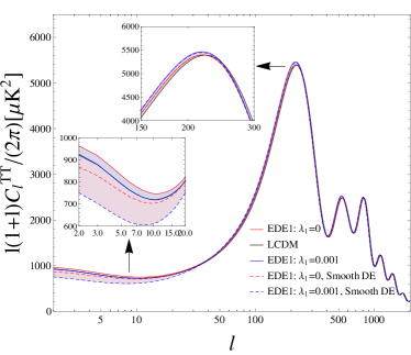
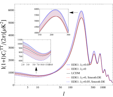
Figure 10: CMB power spectrum for EDE coupled to DM. For EDE models, the solid lines refer to inhomogeneous DE and the dashed lines refer to homogeneous DE.

To disclose the influence of different forms and strength of the interaction , we show the CMB power spectrum for EDE1 with various interactions as well as $\Lambda$CDM in Figure 11. We see that when the interaction is proportional to the density of DM, its influence appears not only at small $l$ but also at the first acoustic peak of the CMB power spectrum. A larger $\lambda_{1}$ accommodates the suppression at low $l$ spectrum but also the enhancement of the first peak. If the interaction is proportional to the energy density of DE, the CMB power spectrum exhibits consistent behaviors both at low $l$ and the first peak: a larger $\lambda_{2}$ leads to the enhancement of the power spectrum. For the EDE models, the influences of the interaction between dark sectors present the same qualitative influence on CMB as compared with the DE with constant EoS 0906.0677 ; 1012.3904 .

Figure 11: CMB power spectrum for EDE1 coupled to DM. For EDE models, the solid lines refer to inhomogeneous DE and the dashed lines refer to homogeneous DE.

IV Fitting results

In this section we fit the EDE models to observations by Markov chain Monte Carlo (MCMC) method. We modify the public code CosmoMCcosmomc1 cosmomc2 to perform the MCMC analysis. For the EDE models without interaction with DM, we carry out the fittings using two datasets: the CMB observations from $Planck$(TT+TE+BB+EE)planck1 ; planck2 ; planck3 and a combined dataset of $Planck$(TT+TE+BB+EE)+BAObao1 bao2 bao3 +SNSN +$H_{0}$H0 . We try to use these observational data to distinguish between homogeneous and inhomogeneous EDE models. When there is interaction between EDE and DM, we fit the EDE models to the combined dataset only, since the CMB data alone cannot constrain the cosmological parameters tightly due to the degeneracy between the coupling strength and DE EoS. In our numerical fittings, the priors of the cosmological parameters are listed in Table 1. For the interaction proportional to the energy density of DM, we have to put strict limits on the priors of the parameters. In order to avoid the negative DE energy density in the early background dynamics and the oscillatory behavior in the time derivative of the gravitational potential, it is necessary that $\lambda_{1}>0$ and $w_{0}>-1$, as we discussed above. For the sake of consistency, we set the prior of $w_{0}$ bigger than $-1$ in all models. Besides, $b$ cannot be close to zero if $\lambda_{1}>0$. Otherwise the DE EoS would be approximately a constant above and close to $-1$ in the early time of the universe, as shown in Figure 1, which is known to cause unstable growth of curvature perturbation0807.3471 ; Xu2011 . Furthermore, considering that CMB power spectrum is more sensitive to $\lambda_{1}$ than $\lambda_{2}$, following 1311.7380 , the prior of $\lambda_{1}$ is tighter than $\lambda_{2}$.

Table 1: The priors for cosmological parameters. $b$(I) refers to the prior of the parameter $b$ of EDE model for no interaction between DM and DE and the interaction proportional to the energy density of DE. $b$(II) refers to the prior for the interaction in proportional to the energy density of DM.

Parameter	Prior
$\Omega_{b}h^{2}$	[0.005, 0.1 ]
$\Omega_{c}h^{2}$	[0.001, 0.5 ]
$100\theta$	[0.5, 10]
$\tau$	[0.01, 0.8]
$n_{s}$	[0.9, 1.1]
$log(10^{10}A_{s})$	[2.7, 4]
$w_{0}$	[-0.99, -0.3]
$b(I)$	[0.0, 1]
$b(II)$	[0.1, 1]
$\lambda_{1}$	[0.0, 0.01]
$\lambda_{2}$	[-0.5, 0.5]

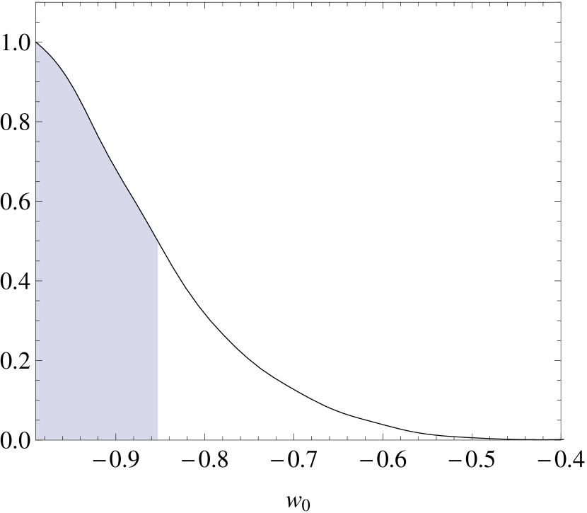
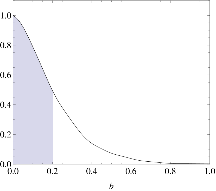
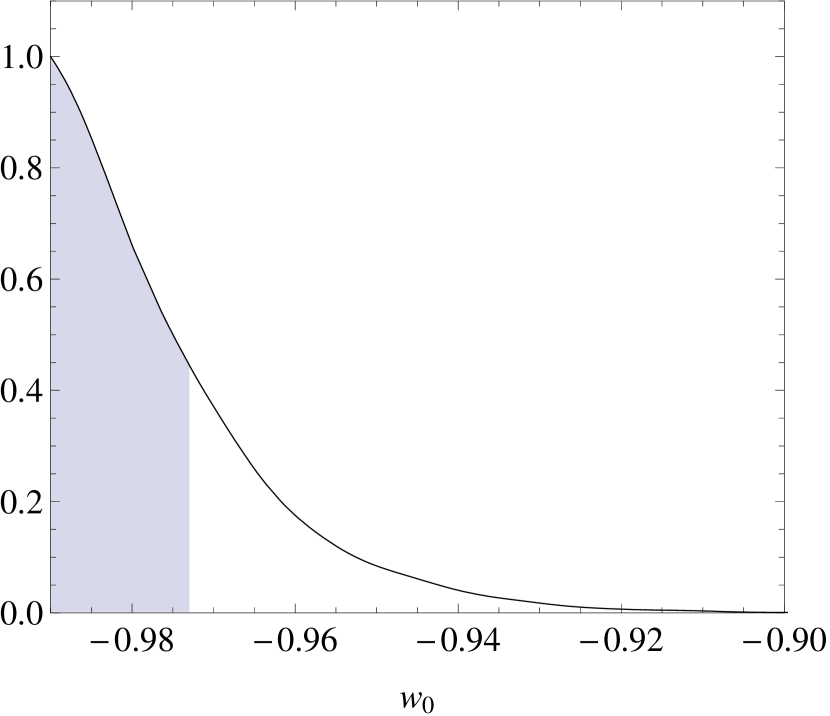
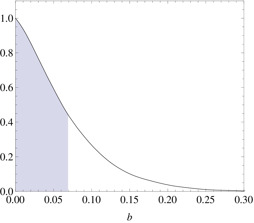
Figure 12: Fitting results of the inhomogeneous EDE model. The upper panel is from the Planck data alone, while the lower panel is from the combined dataset.

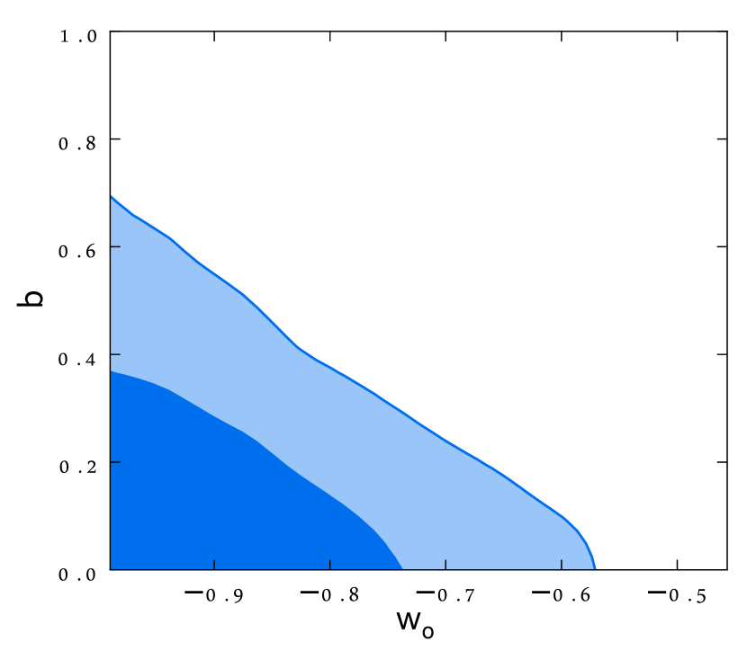
Figure 13: Fitting results of the inhomogeneous EDE model in 2D contour $w_{0}-b$. The left panel is from the Planck data alone, while the right panel is from the combined dataset.

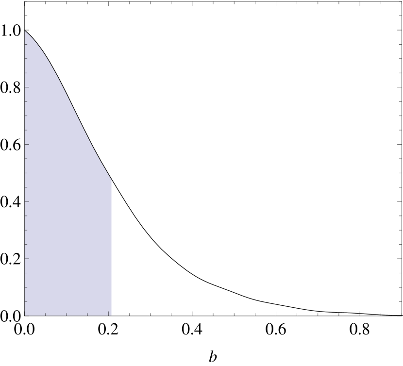
Figure 14: Fitting results of the homogeneous EDE model. The upper panel is from the Planck data alone, while the lower panel is from the combined dataset.

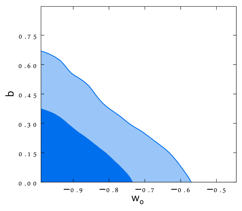
Figure 15: Fitting results of the homogeneous EDE model in 2D contour $w_{0}-b$. The left panel is from the Planck data alone, while the right panel is from the combined dataset.

Table 2: Best fit values and $68\%$ C.L. constraints on the inhomogeneous EDE.

	Planck		Planck+BAO+SN+H0
Parameter	Best-fit	$68\%$ limits	Best-fit	$68\%$ limits
$w_{0}$	$-0.944$	$-0.877^{+0.024}_{-0.113}$	$-0.989$	$-0.975^{+0.002}_{-0.015}$
$b$	$0.111$	$0.171^{+0.033}_{-0.171}$	$0.012$	$0.057^{+0.012}_{-0.057}$
$\chi^{2}$	$9807$		$10243$

Table 3: Best fit values and $68\%$ C.L. constraints on the homogeneous EDE.

	Planck		Planck+BAO+SN+H0
Parameter	Best-fit	$68\%$ limits	Best-fit	$68\%$ limits
$w_{0}$	$-0.886$	$-0.879^{+0.024}_{-0.111}$	$-0.988$	$-0.974^{+0.002}_{-0.016}$
$b$	$0.010$	$0.173^{+0.034}_{-0.173}$	$0.011$	$0.061^{+0.013}_{-0.061}$
$\chi^{2}$	$9806$		$10243$

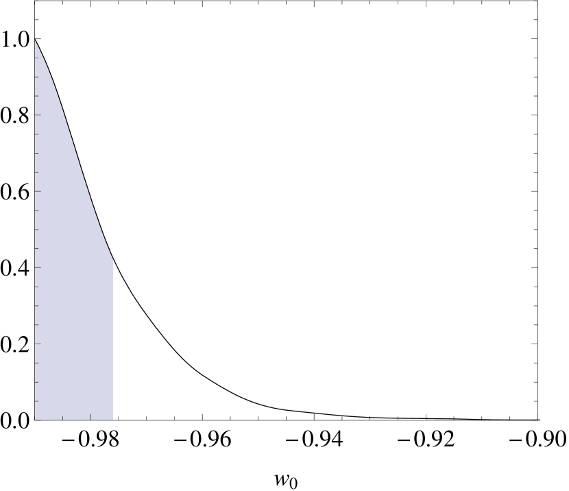
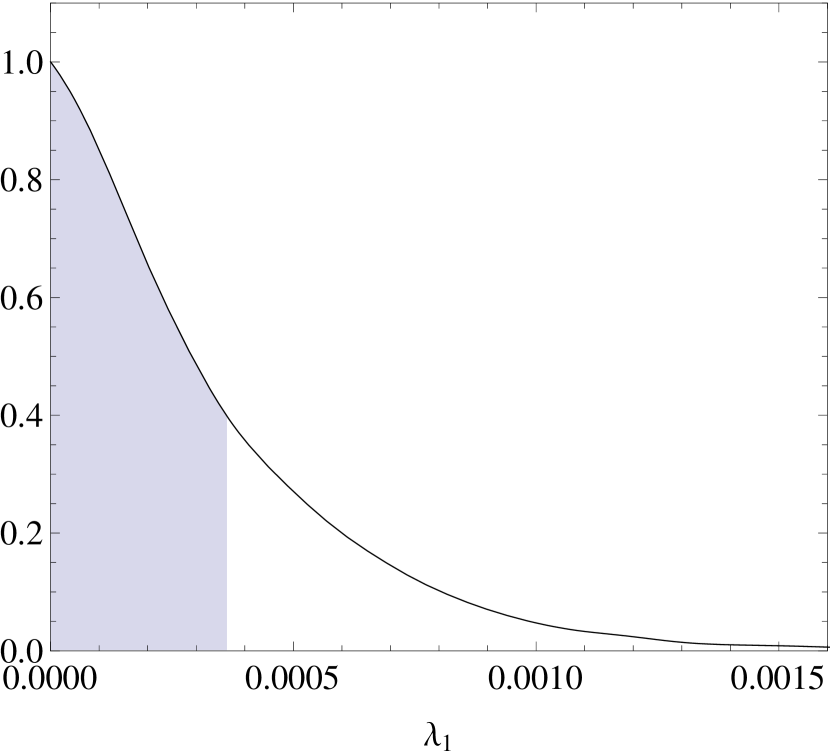
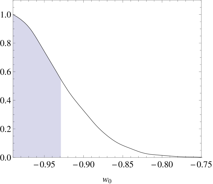
Figure 16: Global fitting results of the inhomogeneous EDE model with interaction. The upper panel is for the interaction proportional to the energy density of DM, while the lower panel is for the interaction proportional to the energy density of DE.

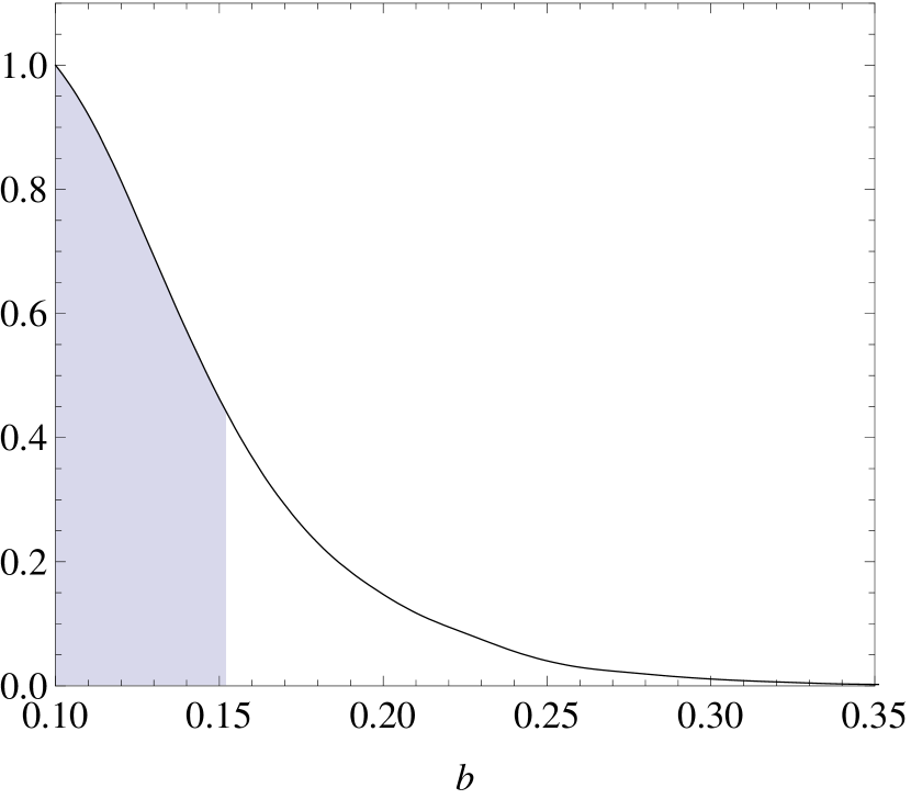
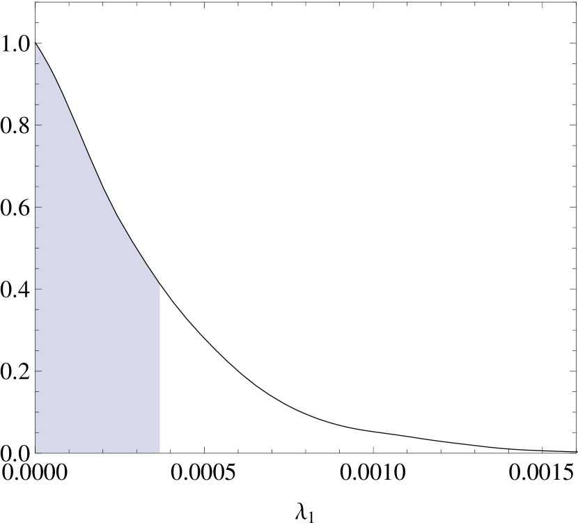
Figure 17: Global fitting results of the homogeneous EDE model with interaction. The upper panel is for the interaction proportional to the energy density of DM, while the lower panel is for the interaction proportional to the energy density of DE.

Table 4: Best fit values and $68\%$ C.L. constraints on inhomogeneous EDE models with interaction using the combined dataset of Planck+BAO+SN+$H_{0}$

	Interaction $\propto\rho_{DM}$		Interaction $\propto\rho_{DE}$
Parameter	Best-fit	$68\%$ limits	Best-fit	$68\%$ limits
$w_{0}$	$-0.985$	$-0.978^{+0.002}_{-0.012}$	$-0.989$	$-0.941^{+0.012}_{-0.049}$
$b$	$0.113$	$0.147^{+0.007}_{-0.047}$	$0.200$	$0.274^{+0.034}_{-0.174}$
$\lambda_{1}$	$0.000274$	$0.000309^{+0.000054}_{-0.000309}$	-	-
$\lambda_{2}$	-	-	$-0.137$	$-0.209^{+0.035}_{-0.050}$
$\chi^{2}$	$10247$		$10238$

Table 5: Best fit values and $68\%$ C.L. constraints on homogeneous models with interaction using the combined dataset of Planck+BAO+SN+$H_{0}$

	Interaction $\sim\rho_{DM}$		Interaction $\sim\rho_{DE}$
Parameter	Best-fit	$68\%$ limits	Best-fit	$68\%$ limits
$w_{0}$	$-0.974$	$-0.977^{+0.002}_{-0.013}$	$-0.966$	$-0.943^{+0.011}_{-0.047}$
$b$	$0.115$	$0.144^{+0.008}_{-0.044}$	$0.123$	$0.282^{+0.038}_{-0.182}$
$\lambda_{1}$	$0.000109$	$0.000311^{+0.000057}_{-0.000311}$	-	-
$\lambda_{2}$	-	-	$-0.189$	$-0.209^{+0.036}_{-0.058}$
$\chi^{2}$	$10248$		$10237$

Figure 18: Ratio of DM energy density to DE energy density of best-fit EDE models.

We first assume that DE and DM evolve independently in the MCMC analysis. For the inhomogeneous EDE, with Planck data alone, we show the results in Table 2. The likelihood distribution for parameters $w_{0}$ and $b$ in the EDE model are shown in the upper panel of Figure 12. Using the combined dataset, we can see how the constraints improve. We list the results in Table 2 and exhibit the likelihood distributions of $w_{0}$ and $b$ in the lower panel of Figure 12. It is easy to see that the addition of the complementary data clearly improves the constraints on the EDE parameters. This is because the parameters which could be degenerate with the EDE parameters, such as the Hubble parameter, are well-constrained by other observations. The 2D contour for $w_{0}$-$b$ is shown in Figure 13.

We then turn to the case where DE perturbations are neglected. Performing an analysis with Planck data alone, we show the fitting results in Table 3 and likelihoods for the EDE model parameters in the upper panel of Figure 14. We find that with Planck data alone, the best-fit of $w_{0}$ is farther away from $-1$ and the best-fit of $b$ gets smaller than the results of the inhomogeneous case. But the mean values and $68\%$ limits are nearly the same. With combined data sets, the best-fit and $68\%$ limit of the inhomogeneous and homogeneous cases shows basically no difference. The 2D contour of $w_{0}$ - $b$ is shown in Figure 15. Both of them suggest that $w_{0}$ is very close to $-1$ and $b$ is small which inmplies tiny EDE effect.

Considering the interaction between DE and DM, we carry out the MCMC analysis again. We display the likelihood distributions of the EDE parameters and the coupling strength from the combined datasets for inhomogeneous and homogeneous EDE in Figure 16 and 17, respectively. The best fitting values and $68\%$ limits are listed in Table 4 and 5. For inhomogeneous EDE with different forms of interaction, the fitting results of $w_{0}$ are similar to that of non-interacting EDE model. On the other hand, we see that in the presence of interaction, the limit of $b$ is larger, which implies that the EDE effect is stronger. This may be attributed to the choice of prior $b$(II). But this tendency is also clear when the interaction is proportional to DE density, which share the same prior of $b$ as non-interacting EDE models.

In the theoretical discussion of the CMB spectrum, we see that the interaction proportional to DM energy density has stronger impact on CMB power spectrum than the interaction proportional to DE energy density. This can be seen also in the fitting results as we find that the limit of $\lambda_{1}$ is much smaller than that of $\lambda_{2}$. The negative best-fit value of $\lambda_{2}$ agrees with the result when DE EoS is constant 1311.7380 . The fitting results for the homogeneous case are similar to the inhomogeneous case.

In the tables of the fitting results, we presented the $\chi^{2}$ for the best-fit models. When the interaction is proportional to the energy density of DM, the prior of $b$ and $\lambda_{1}$ is highly limited as mentioned above. As a result, the $\chi^{2}$ is a bit larger than the non-interacting EDE model. On the contrary, the presence of the interaction proportional to DE density decreases the $\chi^{2}$. Comparing with $\Lambda$CDM model, in which $\chi^{2}=9806,10242$ for $Planck$ and the combined dataset of $Planck$+BAO+SN+$H_{0}$ respectively, we find that the EDE models and its interactions with DM are compatible with current observations.

To examine whether the EDE models allowed by the observations is effective to alleviate the coincidence problem, we plot in Figure 18 the ratio of DM energy density to DE energy density in the best-fit EDE models of the joint analysis and compare them with the $\Lambda$CDM prediction. Comparing the EDE models with $\Lambda$CDM model, we find that if the interaction is proportional to the energy density of DM, the ratio evolves slower than those in other models. By introducing the interaction between dark sectors, the coincidence problem becomes less acute. We conclude that the EDE model is compatible with observations and it is effective to alleviate the coincidence problem.

V conclusions and discussions

In this paper we have studied the influence of EDE on DM perturbations. We have observed that, different from DE models with constant EoS, DM perturbation is larger in inhomogeneous EDE models than in homogeneous EDE model in which DE fluctuation is neglected. We have also disclosed the difference between inhomogeneous and homogeneous EDE in the large scale CMB power spectrum. It is expected that the probe of the growth of large scale structure and small $l$ CMB power spectrum can help to distinguish homogeneous and inhomogeneous EDE models.

Furthermore we have extended our discussion to the interaction between EDE and DM. We have observed that an interaction between EDE and DM also affects DM perturbations and small $l$ CMB power spectrum, which may be degenerate with the effect of DE fluctuations. Comparing these effects, we found that the interaction between EDE and DM has stronger influence on DM perturbations and on the ISW effect.

We have confronted the EDE models to Planck data and a combined dataset of Planck+BAO+SN+$H_{0}$. The analysis showed that the coincidence problem in all best-fit EDE models is less severe than in $\Lambda$CDM model. The positive coupling between EDE and DM proportional to the energy density of DM is particularly effective to alleviate the coincidence problem. This can be clearly seen in Fig. 18 that with the positive coupling between EDE and DM proportional to the energy density of DM, it has longer period for the DE and DM to be comparable.

It is interesting to further examine whether the disclosed impacts of the DE fluctuations and the interaction between DE and DM on observables are specific to EDE models. A lot of efforts on this problem are called for.

- (1) S. Weinberg, Rev. Mod. Phys. 61 1(1989).
- (2) L. P. Chimento, A. S. Jakubi, D. Pavon, and W. Zimdahl, Phys. Rev. D67, 083513 (2003), arXiv: astro-ph/0303145 [astro-ph].
- (3) A. Hojjati, E. V. Linder, J. Samsing, Phys.Rev. Lett111, 041301(2013), arXiv: 1304.3724
- (4) M. Doran, M. Lilley, J. Schwindt, C. Wetterich, ApJ. 559 501(2001)
- (5) U. Alam, ApJ. 714 1460, arXiv: 1003.1259(2010)
- (6) M. Doran, K. Karwan, C. Wetterich, JCAP. 0511 007(2005), arXiv: astro-ph/050813
- (7) P. Wu, H. Yu, Phys. Lett. B643 315(2006), arXiv: astro-ph/0611507
- (8) J. Bielefeld, W.L.Kimmy Wu, R.R. Caldwell, O. Dore, Phys.Rev. D88 103004(2013), arXiv: 1305.2209
- (9) J.Q Xia, M. Viel, JCAP. 0904 002(2009), arXiv: 0901.0605
- (10) C.M. Müller, G. Schäfer, C. Wetterich, Phys.Rev. D70 083504(2004)
- (11) M. Bartelmann, M. Doran, C. Wetterich, A&A, 454 27(2006)
- (12) U. Alam, Z. Lukic, S. Bhattacharya, ApJ. 727 87(2011)
- (13) F. Fontanot, V. Springel, R. E. Angulo, B. Henriques, MNRAS. 426 2335(2012)
- (14) M. Grossi, V. Springel, MNRAS. 394 1559(2009)
- (15) M. Sadegh Movahed, S. Rahvar, Phys. Rev. D73, 083518 (2006)
- (16) Y. G. Gong, Class. Quan. Grav. 22, 2121 (2005)
- (17) R. C. Batista, F. Pace, JCAP. 1306 044(2013)
- (18) S. Das, A. Shafieloo, T. Souradeep, JCAP, 10, 016 (2013), arXiv: 1305.4530
- (19) M. Baldi, MNRAS. 422 1028(2012)
- (20) C. Wetterich, Phys.Lett. B594 17(2004)
- (21) A.A. Costa, X.D. Xu, B. Wang, E.G.M. Ferreira, E. Abdalla, Phys.Rev. D89 103531(2014)
- (22) X.D. Xu, B. Wang, P.J. Zhang, F. Atrio-Barandela, JCAP, 1312 001(2013), arXiv: 1308.1475
- (23) J.H. He, B. Wang, E. Abdalla, Phys.Rev. D83 063515(2011), arXiv: 1012.3904
- (24) J.H. He, B. Wang, E. Abdalla, D. Pavon, JCAP. 1012 022(2010), arXiv: 1001.0079
- (25) E. Abdalla, L. R. W. Abramo, J. Sodre, L., B. Wang, Phys.Lett. B673 107(2009), arXiv: 0710.1198
- (26) E. Abdalla, E.G. M. Ferreira, J. Quintin and Bin Wang, arXiv: 1412.2777
- (27) E. Abdalla, L. Graef, B. Wang, Phys.Lett. B726 786(2012), arXiv: 1202.0499
- (28) S. Micheletti, E. Abdalla, B Wang, Phys.Rev. D79 123506(2009)
- (29) S. Micheletti, JCAP. 1005 009(2010)
- (30) O. Bertolami, P. Carrilho, J. Paramos, Phys.Rev. D86 103522(2012)
- (31) J.H. He, B. Wang, E. Abdalla, Phys.Lett. B671 139(2009), arXiv: 0807.3471
- (32) J.H. He, B. Wang, Y.P. Jing, JCAP. 0907 030(2009), arXiv: 0902.0660
- (33) J.H. He, B. Wang, P.J. Zhang, Phys.Rev. D80 063530(2009), arXiv: 0906.0677
- (34) A. Lewis, A. Challinor, A. Lasenby, Astrophys.J. 538, 473(2000), arXiv: astro-ph/9911177 [astro-ph]
- (35) A. Lewis, S. Bridle, Phys.Rev. D66 103511(2002), arXiv: astro-ph/0205436 [astro-ph]
- (36) A. Lewis, Phys.Rev. D87 103529(2013), arXiv: 1304.4473 [astro-ph.CO]
- (37) Planck Collaboration I. A&A 571, A1(2014), arXiv: 1303.5062
- (38) Planck Collaboration XVI. A&A 571, A16(2014), arXiv: 1303.5076
- (39) Planck Collaboration XV. A&A 571, A15(2014), arXiv: 1303.5075
- (40) F. Beutler, C. Blake, M. Colless, D. H. Jones, L. Staveley-Smith, et al., MNRAS. 416 3017(2011), arXiv: 1106.3366
- (41) N. Padmanabhan, X. Xu, D. J. Eisenstein, R. Scalzo, A. J. Cuesta, et al., MNRAS. 427 2132(2012), arXiv: 1202.0090
- (42) L. Anderson, E. Aubourg, S. Bailey, D. Bizyaev, M. Blanton, et al., MNRAS. 427 3435(2013), arXiv: 1203.6594
- (43) N. Suzuki, D. Rubin, C. Lidman, G. Aldering, R. Amanullah, et al., Apj. 746 85(2012), arXiv: 1105.3470
- (44) A. G. Riess, L. Macri, S. Casertano, H. Lampeitl, H. C. Ferguson, et al., Apj. 730 119(2011), arXiv: 1103.2976
- (45) X.D. Xu, J.H. He and B. Wang, Phys.Lett B 701 (2011) 513 C519, arXiv: 1103.2632