Fluorescence in nonlocal dissipative periodic structures

Abstract

We present an approach for the description of fluorescence from optically active material embedded in layered periodic structures. Based on an exact electromagnetic Green’s tensor analysis, we determine the radiative properties of emitters such as the local photonic density of states, Lamb shifts, line widths etc. for a finite or infinite sequence of thin alternating plasmonic and dielectric layers. In the effective medium limit, these systems may exhibit hyperbolic dispersion relations so that the large wave-vector characteristics of all constituents and processes become relevant. These include the finite thickness of the layers, the nonlocal properties of the constituent metals, and local-field corrections associated with an emitter’s dielectric environment. In particular, we show that the corresponding effects are non-additive and lead to considerable modifications of an emitter’s luminescence properties.

I Introduction

Modern technology relies more and more on the ability of building microscopic devices based on carefully designed nano-structured materials. For example, engineered stacks of differently doped semiconductors are used in modern transistors and (nano-structured) dielectrics with different indices of refraction are used to guide light in the most exotic ways. A special class of nano-structures consists of alternating metallic and insulating layers arranged into one-dimensional periodic lattices. When carefully designed such combinations of plasmonic and dielectric materials lead – within the effective medium limit – to effective hyperbolic dispersion relations Iorsh12 ; Kidwai12 ; Poddubny13 that may be exploited for a number of applications such as subwavelength imaging Belov06 , strong nonlinearities Wurtz11 , emission engineering Cortes12 , and many more. The dispersion relations of these fictitious, spatially uniform hyperbolic meta-materials (HMMs), support radiative modes with infinitely large wave vectors which, in turn, lead to broadband super-singularities of the local photonic density of states DOS (LDOS). It has been recognized that in the actual nano-structure (i.e., without the effective medium description) these singularities become regularized (i) by the fact that for sufficiently large wave-vector values the actual lattice-structure will be resolved Iorsh12 and (ii) via the nonlocal properties of the metallic constituents Iorsh12 ; Yan12 . The LDOS itself can be obtained from the electromagnetic Green’s tensor of the relevant structure. In turn, the LDOS modifies the spontaneous decay rate of an emitter and the corresponding so-called Purcell factor can be determined from the electromagnetic Green’s tensor Yan12 .

Most of the above computations, however, have ignored the effects of local-field corrections in the dielectric layers, despite the fact that these corrections, too, may significantly contribute to the decay dynamics of the emitter. Therefore, in the present work, we include these effects into the Green’s tensor formalism and provide a comprehensive study of the non-additive interplay between the above regularization mechanisms and the local-field corrections on the luminescence properties of emitters embedded in finite-sized and infinitely extended layered HMM-type structures. Besides the aforementioned modified decay rates, this also includes frequency shifts that emitters experience when being embedded in such structures. In addition, we study these effects in the context of different material models for the nonlocal optical properties of the plasmonic constituents and identify analogies and differences in the results.

II Decay Rate and Frequency Shift

The dynamical properties of emitters are correlated with the environment surrounding them. In particular, the decay rates from excited states or the intrinsic transition frequencies depend on the LDOS associated with the electromagnetic environment. Since the latter is strongly correlated with the geometry and the optical properties of the objects filling the space around the emitter, it is not surprising that an appropriate choice of these two characteristics can lead to enhancement or suppression of decay rates as well as to frequency shifts of transitions with respect to their vacuum (empty space) values. Even strong non-Markovian effects can be realized Hoeppe12 . In this section we briefly review the general approach for computing decay rates and frequency shifts of emitters that are embedded in an arbitrary electromagnetic environment.

II.1 Spontaneous decay and local field corrections

We will focus first on the spontaneous decay and calculate the (Purcell) enhancement factor. Within the standard theory for a simple two-level emitter with transition frequency $\Omega$ located at $\mathbf{r}=\mathbf{r}_{0}$, an emitter’s transition rate is given by Wylie84 ; Novotny12

$$\Gamma(\Omega)=\mathrm{Tr}\left[\frac{2\langle\hat{\mathbf{d}}\hat{\mathbf{d}}\rangle}{\hbar}\frac{k_{0}^{2}}{\epsilon_{0}}\mathrm{Im}\left[\underline{G}(\mathbf{r}_{0},\mathbf{r}_{0},\Omega)\right]\right]$$ (1)

Here, $\epsilon_{0}$ and $\hat{\mathbf{d}}$ denote, respectively, the vacuum permittivity and the emitter’s dipole operator while $k_{0}=\Omega/c$ represents the free-space wave vector. The quantum average $\langle.\rangle$ is performed over the emitter’s ground state. The quantity $\underline{G}(\mathbf{r}_{0},\mathbf{r}_{0},\Omega)$ is the electric Green’s tensor, i.e., the solution to the Maxwell equations for an electric point-dipole oscillating with frequency $\Omega$ located at $\mathbf{r}_{0}$ subject to the boundary conditions imposed by the structure surrounding the emitter.

In vacuum the spontaneous decay is well defined and has been studied by many authors. In this case the Green’s tensor is

$$\underline{G}_{0}(\mathbf{r}_{\alpha},\mathbf{r}_{\beta};\omega) =\frac{k_{0}}{4\pi}\bigg{\{}e^{\mathrm{i}k_{0}r_{\alpha,\beta}}\bigg{[}\frac{3\mathbf{n}_{\alpha,\beta}\mathbf{n}_{\alpha,\beta}-1}{k^{3}_{0}r_{\alpha,\beta}^{3}}\left(1-\mathrm{i}k_{0}r_{\alpha,\beta}\right)$$

$$+\frac{1-\mathbf{n}_{\alpha,\beta}\mathbf{n}_{\alpha,\beta}}{k^{3}_{0}r_{\alpha,\beta}^{3}}(k_{0}r_{\alpha,\beta})^{2}\bigg{]}-\frac{4\pi}{3k_{0}^{3}}\delta(\mathbf{r}_{\alpha}-\mathbf{r}_{\beta})\bigg{\}}.$$ (2)

In this expression, we have decomposed the vector $\mathbf{r}_{\alpha}-\mathbf{r}_{\beta}=\mathbf{n}_{\alpha,\beta}\,r_{\alpha,\beta}$ into a unit vector $\mathbf{n}_{\alpha,\beta}$ and a length $r_{\alpha,\beta}$. Equation (2) is nothing but the electromagnetic field emitted by a dipole radiating in vacuum Jackson75 . Using this expression, it is straightforward to show

$$\mathrm{Im}\left[\underline{G}_{0}(\mathbf{r}_{0},\mathbf{r}_{0},\omega)\right] =\frac{k_{0}}{6\pi}$$ (3)

$$\Gamma_{0}(\Omega) =\frac{\langle\langle\hat{d}^{2}\rangle\rangle_{g}}{3\pi\hbar}\frac{k_{0}^{3}}{\epsilon_{0}}=\frac{c}{2\pi\epsilon_{0}}\alpha_{g}k_{0}^{4}.$$ (4)

Here, we have also averaged over the dipole’s direction so that $\langle\hat{d}_{i}\hat{d}_{j}\rangle=\delta_{ij}\langle\langle\hat{d}^{2}\rangle\rangle/3$. In the last term we have used the relation $\alpha_{g}=\frac{2}{3\hbar\omega_{a}}\langle\langle\hat{d}^{2}\rangle\rangle_{g}$ that connects the ground-state and angle-averaged dipole moment with the static polarizability $\alpha_{g}$. When the dipole is instead embedded in a homogeneous dielectric medium, things are, however, more complicated. The corresponding Green’s tensor can be obtained by the formal replacement $k_{0}\to k_{h}=\sqrt{\epsilon(\Omega)}k_{0}$ where $\epsilon(\Omega)$ is the dielectric function describing the medium. From simple considerations, one would expect that $\Gamma(\Omega)=\mathrm{Re}[\sqrt{\epsilon(\Omega)}]\Gamma_{0}(\Omega)$. In reality, in a naive application of Eq.(1), with the Green’s tensor given by Eq.(2) for a homogeneous dielectric medium, even a minute amount of dissipation would lead to a divergent decay rate. Physically, this difficulty can be understood by thinking that in a continuum approximation, resulting from a macroscopic average, the emitter can superpose with an atom of the dielectric leading to a divergent interaction Fleischhauer99 . The spontaneous decay of an emitter embedded in a dielectric medium thus represents an example of how dissipation can substantially complicate the theory of quantum phenomena.

For the realistic description of spontaneous decay processes we have to take into account that the electromagnetic field “seen” by an emitter that is embedded in a medium is not given by solutions of the macroscopic Maxwell equations. Rather, the fields provided by macroscopic electrodynamics are the result of spatial averages where materials are described as continuous entities characterized by permittivities and permeabilityies. At the microscopic level the “granular” structure of the medium becomes important and the local field felt by the emitter can be rather different from the result of the macroscopic averaging procedure. In turn, this may have a very significant impact on the emitters’ dynamics, notably if they are exposed to multiple scattering effects originating from a complex nano-structured environment. In order to treat the local-field problem, one can distinguish two different cases Glauber91 ; Vries98 ; Scheel99a ; Scheel99 ; Fleischhauer99 : (a) The emitter is of the same species as the atoms (or molecules) that constitute the host medium or (b) the emitter is of a different species as the host medium, i.e., an impurity, a substitution etc. In both cases (and even for non-dissipative media), the spontaneous decay is non-trivially modified with respect to the result for vacuum presented above. The first scenario is described within the virtual-cavity model Vries98 ; Scheel99a ; Scheel99 ; Fleischhauer99 , where the Green’s tensor is appropriately modified to remove all unphysical divergences. The second scenario is treated within the Onsager real-cavity model where the emitter is thought to be placed in vacuum at the center of a spherical cavity carved into the host medium Glauber91 ; Vries98 ; Scheel99a ; Scheel99 ; Tomas01 ; Dung06 , where the cavity radius is essentially given by the distance to the next atom (molecule) of the dielectric (see Fig. 1). In the present work, we will restrict ourselves to systems for which the real-cavity model may be applied.

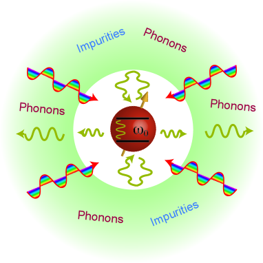
Figure 1: (Color online) Within the real-cavity model the emitter is placed in vacuum and a spherical cavity is carved inside the host dielectric material. This is a simple description of realistic situation where the emitter is embedded into the lattice formed by the atoms (molecules) of the host material Vries98 . The cavity radius is determind by the average distance between the emitter and the nearest atoms (molecules) of the host material.

Before describing how Eq. (1) has to be modified in order to include the local-field correction, we first consider the impact of multiple scattering effects by complex nano-structured systems on the electromagnetic Green’s tensor. If all media are linear, we have that

$$\underline{G}(\mathbf{r}_{0},\mathbf{r}_{0};\omega)=\underline{G}_{h}(\mathbf{r}_{0},\mathbf{r}_{0};\omega)+\underline{G}_{s}(\mathbf{r}_{0},\mathbf{r}_{0};\omega),$$ (5)

where the tensor $\underline{G}_{h}$ describes the propagation of the electromagnetic field within a homogeneous medium with the same permittivity and permeability as the medium at position $\mathbf{r}_{0}$. Within the real-cavity model this allows us to identify vacuum as the homogeneous medium required for the homogeneous Green’s tensor, i.e., we have $\underline{G}_{h}=\underline{G}_{0}$. Further, the tensor $\underline{G}_{s}$ represents the scattered Green’s tensor and takes into account the multiple scattering processes due to the material interfaces in the nano-structure. For simple geometries the expressions for $\underline{G}_{s}$ are well-known and have been reported in the literature (we refer to Wylie84 ; Wylie85 ; Jackson75 ; Tomas95 and our discussion of layered systems below). In the local-field corrected Green’s tensor within the framework of the real-cavity model, the emitter is placed in vacuum enclosed at the center of a spherical cavity with radius $R$ much smaller than the optical wavelength ($k_{0}R\ll 1$). In our specific case of alternating metallic and dielectric layers, this spherical local-field cavity with the emitter in its center is located inside a central dielectric layer with permittivity $\epsilon(\omega)$ sandwiched between a finite or infinite number of further layers on either side. This means that the scattering Green’s tensor $\underline{G}_{s}$ is determined from both, the boundary conditions on the cavity sphere and on interfaces between the layers. Clearly, these two sets of boundary conditions act in a very non-additive way, thus complicating the evaluation of the Green’s tensor. Fortunately, this topic has been extensively discussed in the literature Tomas01 ; Dung06 ; Sambale07 ; Scheel08 so that we may directly utilize that in this case the scattered Green’s tensor can be written as

$$\underline{G}_{s}(\mathbf{r}_{0},\mathbf{r}_{0};\omega)=C(\omega,R)\frac{k_{0}}{6\pi}+S^{2}(\omega,R)\,\underline{\mathcal{G}}_{s}(\mathbf{r}_{0},\mathbf{r}_{0};\omega)$$ (6)

Here, $\underline{\mathcal{G}}_{s}$ is the scattered Green’s tensor that exclusively results from the multiple scattering at the layers’ interfaces and the effect of the spherical cavity appears in two terms: An offset $C(\omega,R)$ that will survive even if we remove all the scattering from all layers and a prefactor $S^{2}(\omega,R)$ to the scattering Green’s tensor $\underline{\mathcal{G}}_{s}$ that account for the multiple scattering at layer interfaces. This specific structure of the full scattering Green’s tensor $\underline{G}_{s}$ makes quite explicit the non-additive character of the local-field and the multiple-scattering corrections. Within the real-cavity model, we have Tomas01 ; Dung06 ; Sambale07 ; Scheel08

$$C(\omega,R)= \frac{h^{(1)}_{1}(\nu_{0})[\nu h^{(1)}_{1}(\nu)]-\epsilon(\omega)[h^{(1)}_{1}(\nu_{0})\nu_{0}]^{\prime}h^{(1)}_{1}(\nu)}{\epsilon(\omega)h^{(1)}_{1}(\nu)[\nu_{0}j_{1}(\nu_{0})]^{\prime}-[h^{(1)}_{1}(\nu)\nu]^{\prime}j_{1}(\nu_{0})}$$ (7)

$$S(\omega,R)= \frac{j_{1}(\nu_{0})[\nu_{0}h^{(1)}_{1}(\nu_{0})]^{\prime}-[j_{1}(\nu_{0})\nu_{0}]^{\prime}h^{(1)}_{1}(\nu_{0})}{j_{1}(\nu_{0})[\nu h^{(1)}_{1}(\nu)]^{\prime}-\epsilon(\omega)[j_{1}(\nu_{0})\nu_{0}]^{\prime}h^{(1)}_{1}(\nu)}$$ (8)

where we have introduced the abbreviations $\nu_{0}=k_{0}R$ and $\nu=k_{0}\sqrt{\epsilon(\omega)}R$ while $j_{1}(\nu)$ and $h^{(1)}_{1}(\nu)$ denote, respectively, the spherical Bessel function of order one and the spherical Hankel function of the first kind of order one (the prime indicates the derivative with respect to the argument of the corresponding Bessel/Hankel functions). We would like to emphasize that $\nu$ and, consequently, also the wave vector of the dielectric host medium $k_{h}=k_{0}\sqrt{\epsilon(\omega)}$ are complex valued due to the fact that the host medium’s permittivity $\epsilon(\omega)$ is, in general, complex valued. Also, as a result of the foregoing, the spontaneous decay formally depends on an external parameter, i.e., the cavity radius $R$. As stated above, this parameter is fixed by the microscopic arrangement of the host dielectric atoms and must be experimentally determined. However, for optical frequencies, one may even consider an expansion of the above expressions in the small parameter $k_{0}R\ll 1$(see Refs. Tomas01 ; Dung06 ; Sambale07 ; Scheel08 ).

Upon averaging over the emitter’s dipole orientations, the local-field corrected emission rate is given by

$$\Gamma(\Omega) =\frac{1}{3}\,\mathrm{Tr}[\underline{H}_{\rm P}]\,\Gamma_{0}(\Omega),$$ (9)

where we have introduced the tensor

$$\underline{H}_{\rm P} =1+\mathrm{Im}[C(\Omega,R)]$$

$$+\frac{6\pi}{k_{0}}\mathrm{Im}\left[S^{2}(\Omega,R)\,\underline{\mathcal{G}}_{s}(\mathbf{r}_{0},\mathbf{r}_{0};\Omega)\right].$$ (10)

The last step in our approach is the determination of $\underline{\mathcal{G}}_{s}$, for which we have to specify the arrangement of layers. In this work, we consider one central dielectric layer containing the emitter that is symmetrically sandwiched by a finite or infinite number of identical bilayers that consist of one plasmonic and one dielectric material. For simplicity, we restrict ourselves to the case where all dielectric layers are made from the same material (see Fig. 2). From the emitter’s point of view, the structure resembles a cavity that is formed by two Bragg mirrors and is filled with a dielectric material with permittivity $\epsilon(\omega)$. We align the $z$-direction with the stacking direction of the layers and denote the emitter’s distance from the nearest plasmonic layer with $d$. Further, the left and right Bragg mirror are, respectively, labeled with indices “1” and “2”. Then, we may decompose the scattering Green’s tensor $\underline{\mathcal{G}}_{s}$ into components parallel and perpendicular to the stacking direction of the layers

$$\underline{\mathcal{G}}_{s}(\mathbf{r}_{0},\mathbf{r}_{0};\omega) \equiv\underline{\mathcal{G}}_{s}(d,\omega)$$

$$=\mathcal{G}_{\|}(d,\omega)(\mathbf{x}\mathbf{x}+\mathbf{y}\mathbf{y})+\mathcal{G}_{\bot}(d,\omega)\mathbf{z}\mathbf{z}.$$ (11)

In turn, the parallel and perpendicular components of the Green’s tensor, $\mathcal{G}_{\|}$ and $\mathcal{G}_{\bot}$, may be expressed through the structure’s geometrical parameters and the (frequency- and wave-vector dependent) reflection coefficients $r^{\sigma}_{1}$, and $r^{\sigma}_{2}$ ($\sigma=s,p$) of the two Bragg mirrors for s- and p-polarized plane waves. Specifically, if $D$ is the cavity length, these components of the Green’s tensor read as Tomas95

$$\mathcal{G}_{\|}(d,\omega)=\frac{1}{8\pi}\int_{0}^{\infty}dk\,\frac{k\,\kappa_{\rm lc}}{k_{h}^{2}} \left[\frac{r^{p}_{1}e^{-2\kappa_{\rm lc}d}+r^{p}_{2}e^{-2\kappa_{\rm lc}(D-d)}-2r^{p}_{1}r^{p}_{2}e^{-2\kappa_{\rm lc}D}}{1-r^{p}_{1}r^{p}_{2}e^{-2\kappa_{\rm lc}D}}\right.$$

$$+ \left.\frac{k_{h}^{2}}{\kappa_{\rm lc}^{2}}\frac{r^{s}_{1}e^{-2\kappa_{\rm lc}d}+r^{s}_{2}e^{-2\kappa_{\rm lc}(D-d)}+2r^{s}_{1}r^{s}_{2}e^{-2\kappa_{\rm lc}D}}{1-r^{s}_{1}r^{s}_{2}e^{-2\kappa_{\rm lc}D}}\right],$$ (12a)

$$\mathcal{G}_{\bot}(d,\omega)=\frac{1}{8\pi}\int_{0}^{\infty}dk\,\frac{k\,\kappa_{\rm lc}}{k_{h}^{2}}\,\left[2\frac{k^{2}}{\kappa_{\rm lc}^{2}}\frac{r^{p}_{1}e^{-2\kappa_{\rm lc}d}+r^{p}_{2}e^{-2\kappa_{\rm lc}(D-d)}+2r^{p}_{1}r^{p}_{2}e^{-2\kappa_{\rm lc}D}}{1-r^{p}_{1}r^{p}_{2}e^{-2\kappa_{\rm lc}D}}\right],$$ (12b)

where $\kappa_{\rm lc}=\sqrt{k^{2}-k_{h}^{2}}=-\mathrm{i}k_{\rm lc}$. For our symmetric geometry, the reflection coefficients of the Bragg mirrors are identical so that $r^{s}_{1}=r^{s}_{2}=r^{s}$ and $r^{p}_{1}=r^{p}_{2}=r^{p}$. For simplicity, we will subsequently restrict ourselves to the case of $D=2d$ so that the emitter is located at the center of the cavity (see Fig. 2). The complete determination of the scattered Green’s tensor components requires the evaluation of the reflection coefficient $r^{\sigma}$ which will be the subject of the section III.

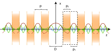
Figure 2: (Color online) Sketch of the layered material considered in this work. A central dielectric layer (thickness $D$, white shading) is sandwiched between a finite or infinite number of identical bilayers (total thickness $p=p_{1}+p_{2}$) consisting of a plasmonic (thickness $p_{2}$, red shading) and a dielectric layer (thickness $p_{1}$, white shading). All dielectric layers are made from the same material (permittivity $\epsilon(\omega)$). The plasmonic layers are identical and different material models are considered. For the infinite system, the dashed region delineates the unit cell. See text for further details.

II.2 Frequency shift

In addition to the spontaneous decay rate, modifications of the electromagnetic environment as well as local-field corrections have an impact on the emitter’s energy levels. The treatment of this effect leverages on the same tools as discussed above, i.e., the determination of the Green’s tensor. For a two-level emitter the standard approach relies on the connection between the Casimir-Polder energy ($U_{\rm CP}$) Intravaia11 ; Haakh13 and the change in the emitter’s ground state energy ($\Delta E_{g}$) Wylie84 ; Wylie85 : $U_{\rm CP}=\Delta E_{g}\equiv\hbar\Delta\omega_{g}$. (This connection can also be generalized to higher energy levels Wylie84 ; Wylie85 .) If $\underline{\alpha}(\omega)$ is the ground-state polarizability, the Casimir-Polder energy is given by

$$U_{\rm CP}=\hbar\int_{0}^{\infty}\frac{d\xi}{2\pi\epsilon_{0}}\mathrm{Tr}\left[\underline{\alpha}(\mathrm{i}\xi)\cdot\frac{\xi^{2}}{c^{2}}\underline{G}_{s}(\mathbf{r}_{0},\mathbf{r}_{0};\mathrm{i}\xi)\right],$$ (13)

where we have used the local-field corrected expression (6) for the scattered Green’s tensor. For a two-level emitter and after averaging over the emitter’s dipole direction, we obtain

$$\underline{\alpha}(\mathrm{i}\xi)=\alpha(\mathrm{i}\xi)\underline{1}=\alpha_{g}\frac{\Omega^{2}}{\xi^{2}+\Omega^{2}}\underline{1}\,,$$ (14)

where $\underline{1}$ denotes the unit tensor. Within the framework of second-order perturbation theory Wylie84 ; Wylie85 ; Intravaia11 the above expression is equivalent to an additional contribution to the vacuum-induced Lamb shift of the ground state energy that is generated by the nano-structure. From Eq.(6), we obtain two distinct contributions. The first is exclusively associated with the local-field correction

$$U^{(1)}_{\rm CP}=3\hbar\int_{0}^{\infty}\frac{d\xi}{2\pi\epsilon_{0}}\,\alpha(\mathrm{i}\xi)\frac{\xi^{2}}{c^{2}}G_{\rm C}(\mathrm{i}\xi,R),$$ (15)

where

$$G_{\rm C}(\omega,R)=C(\omega,R)\frac{k_{0}}{6\pi}.$$ (16)

The second contribution

$$U^{(2)}_{\rm CP}=\hbar\int_{0}^{\infty}\frac{d\xi}{2\pi\epsilon_{0}}\,\alpha(\mathrm{i}\xi)\,S^{2}(\mathrm{i}\xi,R)\mathrm{Tr}\left[\underline{\mathcal{G}}_{s}(d,\mathrm{i}\xi)\right],$$ (17)

describes the impact of the Bragg mirrors on the shift and, therefore, depends on the detailed characteristics of the structure such as the distance of the emitter from the dielectric/metal interfaces etc. In the following, we will exclusively focus on this second contribution, since for a specific dielectric it is the only one that can be tuned as a function on the geometric parameters of the surrounding nano-structure Sambale07 .

III Periodic Structures: Bloch equation and Scattering Coefficients

The behavior of the electromagnetic field within a periodic structure can be analyzed in the framework of the Bloch theorem Busch07 . If the periodic medium is composed of a stacking sequence of layers, the problem can be tackled analytically with the help of a transfer-matrix approach Yeh77 ; Yariv83 . Specifically, the continuity of the transverse field components leads to boundary conditions across each layer. For the metallic layer, we have (c.f. Fig. 2)

$$\begin{pmatrix}E\\ cB\end{pmatrix}_{z=\frac{p_{1}}{2}+p_{2}}^{\sigma}=\mathbb{M}^{\sigma}_{\rm nl}(p_{2})\begin{pmatrix}E\\ cB\end{pmatrix}_{z=\frac{p_{1}}{2}}^{\sigma},$$ (18)

while for the dielectric layer, we obtain

$$\begin{pmatrix}E\\ cB\end{pmatrix}_{z=\frac{p_{1}}{2}+p}^{\sigma}=\mathbb{M}^{\sigma}_{\rm lc}(p_{1})\begin{pmatrix}E\\ cB\end{pmatrix}_{z=\frac{p_{1}}{2}+p_{2}}^{\sigma}.$$ (19)

Here, $\sigma=s,p$ indicates again the polarization while $\mathbb{M}^{\sigma}_{\rm nl}\left(p_{2}\right)$ and $\mathbb{M}^{\sigma}_{\rm lc}\left(p_{1}\right)$ represent the transfer matrices associated with each layer. Specifically, as we will exclusively consider spatially local material models for the dielectric, we have introduced the subscript “lc” for dielectric layer transfer matrices. Similarly, as we will mainly focus on spatially nonlocal material models for the metal, we have introduced the subscript “nl” for metal layer transfer matrices. Further, the propagation across a bilayer can be written as

$$\begin{pmatrix}E\\ cB\end{pmatrix}_{z=\frac{p_{1}}{2}+p}^{\sigma}=\mathbb{T}^{\sigma}\begin{pmatrix}E\\ cB\end{pmatrix}_{z=\frac{p_{1}}{2}}^{\sigma},$$ (20)

where the corresponding transfer matrix $\mathbb{T}$ is given by

$$\mathbb{T}^{\sigma}=\mathbb{M}^{\sigma}_{\rm nl}\left(p_{2}\right)\mathbb{M}^{\sigma}_{\rm lc}\left(p_{1}\right).$$ (21)

For a local dielectric material, the transfer matrix $\mathbb{M}^{\sigma}_{\rm lc}\left(p_{1}\right)$ can be written as

$$\mathbb{M}^{\sigma}_{\rm lc}\left(p_{1}\right)=\begin{pmatrix}\cos(k_{\rm lc}p_{1})&\mathrm{i}\delta^{\sigma}\sin(k_{\rm lc}p_{1})Z^{\sigma}_{\rm lc}\\ \mathrm{i}\delta^{\sigma}\sin(k_{\rm lc}p_{1})/Z^{\sigma}_{\rm lc}&\cos(k_{\rm lc}p_{1})\end{pmatrix},$$ (22)

where, for p- and s-polarization, respectively, we have $\delta^{p}=1$ and $\delta^{s}=-1$. Further, we have defined the local surface impedances

$$Z_{\rm lc}^{p}=\frac{ck_{\rm lc}}{\omega\epsilon(\omega)},\quad\mbox{and}\quad Z_{\rm lc}^{s}=\frac{\omega}{ck_{\rm lc}}.$$ (23)

In the case of a metallic layer with nonlocal material model the entries of $\mathbb{M}_{\rm nl}(p_{2})$ depends on the specific model used to describe the nonlocality (see section IV). Nevertheless, the matrix has a similar structure as in the local case

$$\mathbb{M}^{\sigma}_{\rm nl}\left(p_{2}\right)=\begin{pmatrix}\mathrm{cs}^{\sigma}_{\rm nl}(p_{2})&\mathrm{i}\delta^{\sigma}\mathcal{Z}^{\sigma}_{\rm right}(p_{2})\\ \mathrm{i}\delta^{\sigma}/\mathcal{Z}^{\sigma}_{\rm left}(p_{2})&\mathrm{cs}_{\rm nl}(p_{2}),\end{pmatrix}$$ (24)

with functions $\mathrm{cs}^{\sigma}_{\rm nl}(p_{2})$, $\mathcal{Z}^{\sigma}_{\rm left}(p_{2})$ and $\mathcal{Z}^{\sigma}_{\rm left}(p_{2})$ that have to be determined from the specific material model. For instance, reciprocity stipulates that both matrices $\mathbb{M}^{\sigma}_{\rm nl}\left(p_{2}\right)$ and $\mathbb{M}^{\sigma}_{\rm lc}\left(p_{1}\right)$ have a determinant equal to one. While this clearly is fulfilled for $\mathbb{M}_{\rm lc}(p_{1})$, this condition imposes certain restriction to the general form describing the non-local case

$$\frac{\mathcal{Z}_{\rm right}(p_{2})}{\mathcal{Z}_{\rm left}(p_{2})}+\mathrm{cs}^{2}_{\rm nl}(p_{2})=1.$$ (25)

III.1 Infinite Bragg Mirrors

In an infinite periodic structure the Bloch theorem further requires that the field values across a unit cell satisfy

$$\begin{pmatrix}E\\ cB\end{pmatrix}_{z=\frac{p_{1}}{2}+p}=e^{\mathrm{i}\alpha p}\begin{pmatrix}E\\ cB\end{pmatrix}_{z=\frac{p_{1}}{2}}\leavevmode\nobreak\ .$$ (26)

This leads to an eigenvalue equation $\mathbb{T}=e^{\mathrm{i}\alpha p}$ that connects the eigenvalues with the generally complex values of the Bloch vector $\alpha$. Since $\mathrm{Det}[\mathbb{T}]=1$, the eigenvalues have the form $e^{\pm\mathrm{i}\alpha p}$ and using the invariance of the trace of a matrix we obtain the generalized Bloch equation

$$\cos(\alpha p)=\cos(k_{\rm lc}p_{1})\mathrm{cs}_{\rm nl}(p_{2})\\ -\frac{1}{2}\sin(k_{\rm lc}p_{1})\left(\frac{Z_{\rm lc}}{\mathcal{Z}_{\rm left}(p_{2})}+\frac{\mathcal{Z}_{\rm right}(p_{2})}{Z_{\rm lc}}\right),$$ (27)

where, for simplicity of notation, we have dropped the polarization superscript. For the computation of the scattering Green’s tensor, we require the reflection coefficients from infinitely extended half-spaces and this can be derived in terms of the eigenvector of the transfer matrix Mochan87 ; Yariv83 : Each of the two eigenvectors corresponds to a Bloch mode propagating either to the right or to the left of the unit cell. The components of the mode are the corresponding electric and magnetic fields from which it is possible to derive the surface impedance $Z_{\rm per}$ for the periodic structure Mochan87 . We obtain

$$Z_{\rm per}=-\frac{\mathbb{T}_{12}}{\mathbb{T}_{11}-e^{\mathrm{i}\alpha p}}=-\frac{\mathbb{T}_{22}-e^{\mathrm{i}\alpha p}}{\mathbb{T}_{21}},$$ (28)

which, upon inserting the specific form of the transfer matrices, explicitly reads as

$$Z_{\rm per} =\mathrm{i}\mathcal{Z}_{\rm right}\frac{\cos(k_{\rm lc}p_{1})+\frac{Z_{\rm lc}}{\mathcal{Z}_{\rm left}}\mathrm{cs}_{\rm nl}(p_{2})\sin(k_{\rm lc}p_{1})}{e^{\mathrm{i}\alpha p}-\cos(k_{\rm lc}p_{1})\mathrm{cs}_{\rm nl}(p_{2})+\sin(k_{\rm lc}p_{1})\frac{\mathcal{Z}_{\rm right}}{Z_{\rm lc}}}$$

$$=-\mathrm{i}\mathcal{Z}_{\rm left}\frac{e^{\mathrm{i}\alpha p}-\cos(k_{\rm lc}p_{1})\mathrm{cs}_{\rm nl}(p_{2})+\sin(k_{\rm lc}p_{1})\frac{Z_{\rm lc}}{\mathcal{Z}_{\rm left}}}{\cos(k_{\rm lc}p_{1})+\frac{\mathcal{Z}_{\rm left}}{Z_{\rm lc}}\mathrm{cs}_{\rm nl}(p_{2})\sin(k_{\rm lc}p_{1})},$$ (29)

where, again, the polarization superscript has been suppressed. The reflection coefficients for infinite periodic Bragg mirrors can then be written as

$$r^{p}=\frac{Z^{p}_{\rm lc}-Z^{p}_{\rm per}}{Z^{p}_{\rm lc}+Z^{p}_{\rm per}},\quad\mbox{and}\quad r^{s}=-\frac{Z^{s}_{\rm lc}-Z^{s}_{\rm per}}{Z^{s}_{\rm lc}+Z^{s}_{\rm per}}.$$ (30)

III.2 Finite Bragg Mirrors

The transfer matrix $\mathbb{T}$ can also be utilized for obtaining the reflection coefficients for structures with a finite number of bilayers Yeh77 ; Yariv83 embedded into half-spaces of the host dielectric materials. For a single metallic layer (i.e., a slab) with thickness $p_{2}$ the reflection and transmission coefficients, $r_{\rm slab}^{\sigma}$ and $t_{\rm slab}^{\sigma}$, are given by

$$r_{\rm slab}^{\sigma}=\delta^{\sigma}\frac{Z^{2}_{\rm lc}-Z_{\rm right}(p_{2})Z_{\rm left}(p_{2})}{Z^{2}_{\rm lc}+Z_{\rm right}(p_{2})Z_{\rm left}(p_{2})+2\mathrm{i}\,\mathrm{cs}_{\rm nl}(p_{2})Z_{\rm lc}Z_{\rm left}}$$ (31)

$$t_{\rm slab}^{\sigma}=\frac{2\mathrm{i}Z_{\rm lc}Z_{\rm left}(p_{2})}{Z_{\rm lc}^{2}+Z_{\rm right}(p_{2})Z_{\rm left}(p_{2})+2\mathrm{i}\,\mathrm{cs}_{\rm nl}(p_{2})Z_{\rm lc}Z_{\rm left}(p_{2})}.$$ (32)

Here, again, the polarization superscript has been suppressed. The expression for the reflection coefficients of a finite structure composed of a sequence of $N$ can then be written as Yeh77 ; Yariv83

$$r^{\sigma}_{N}=\frac{r^{\sigma}_{\rm slab}e^{2\mathrm{i}k_{\rm lc}p_{1}}}{1-t^{\sigma}_{\rm slab}e^{\mathrm{i}k_{\rm lc}p_{1}}\frac{\sin([N-1]\alpha p)}{\sin(N\alpha p)}},$$ (33)

where, we recall that $\alpha$ is the Bloch vector.

IV The Description of Nonlocal Media

The description of the nonlocal properties of metals has been the subject of many publications in the past (we refer to Ford84 for an overview of earlier works) and, in the context of nano-plasmonics, has recently experienced renewed interests. Here, we give a brief review of two different models which have been formulated in the literature and provide the results that are required for our computations.

IV.1 The SCIB Model

We first consider the approach which goes under the name of semi-classical infinite barrier (SCIB) model Feibelman82 ; Ford84 , that has been utilized for the description of the anomalous skin effect Kliewer68 ; Jones69 ; Fuchs69 . In the SCIB model, the interface is described very crudely through an infinite barrier but it takes into account the most relevant physical phenomena inside the metal Feibelman82 ; Ford84 . Within this approach, the electrons are treated as a classical ideal gas that is governed by the Fermi-Dirac statistics and whose dynamics is described via the Boltzmann equation. It is further assumed that the electrons in this nonlocal medium specularly reflect at the interface with another medium Horovitz12 . It has been shown that the fields in the interior of such a nonlocal medium, are identical to the fields that arise from a current sheet source at the surface. Since in our case, the system is invariant with respect to translations in the $x-y$ plane and an interface is located at $z=z_{0}$ this sheet current has the form (we follow the notation of Ref. Ford84 )

$$\mathbf{j}(\mathbf{r},t)=\mathbf{J}\delta(z-z_{0})e^{\mathrm{i}(\mathbf{k}\cdot\mathbf{R}-\omega t)}\quad\text{ with }\quad\mathbf{J}\cdot\mathbf{z}=0,$$ (34)

where $\mathbf{k}$ is the component of the wavevector orthogonal to the $z$-direction ($\mathbf{z}$ denotes the unit vector along the $z$-direction). The corresponding electric field has the form

$$\mathbf{E}(\mathbf{r},t)=\mathbf{E}(z)e^{\mathrm{i}(\mathbf{k}\cdot\mathbf{R}-\omega t)}$$ (35)

and an analoguous expression holds for the magnetic field. If $\mathbf{K}=(\mathbf{k},k_{z})$ is the three-dimensional wave vector, the dielectric tensor of the metal within SCIB can be written as

$$\underline{\epsilon}(K,\omega)=\epsilon_{l}(K,\omega)\frac{\mathbf{K}\mathbf{K}}{K^{2}}+\epsilon_{t}(K,\omega)\frac{K^{2}\underline{1}-\mathbf{K}\mathbf{K}}{K^{2}}.$$ (36)

The Maxwell equations can then be solved in terms of the longitudinal and transverse dielectric functions, $\epsilon_{l}(K,\omega)$ and $\epsilon_{t}(K,\omega)$, respectively, and we obtain that the component of the electric and magnetic field parallel to the layer interface can be written as

$$E_{nl}^{p}(z) =-\frac{Z_{0}}{2}\hat{\mathbf{k}}\cdot\mathbf{J}\eta^{p}(z-z_{0})$$ (37)

$$B_{nl}^{p}(z) =-\frac{Z_{0}}{2c}\hat{\mathbf{k}}\cdot\mathbf{J}\beta(z-z_{0})$$ (38)

$$E_{nl}^{s}(z) =-\frac{Z_{0}}{2}(\hat{\mathbf{z}}\times\hat{\mathbf{k}})\cdot\mathbf{J}\eta^{s}(z-z_{0})$$ (39)

$$B_{nl}^{s}(z) =\frac{Z_{0}}{2c}(\hat{\mathbf{z}}\times\hat{\mathbf{k}})\cdot\mathbf{J}\beta(z-z_{0})$$ (40)

where $Z_{0}=\sqrt{\mu_{0}/\epsilon_{0}}$ is the vacuum impedance and the dimensionless functions $\eta(z)$ and $\beta(z)$ are defined as

$$\eta^{p}(z)=\frac{\omega}{c}\int_{-\infty}^{\infty}\frac{dk_{z}}{2\pi\mathrm{i}}\left(\frac{2\frac{k_{z}^{2}}{K^{2}}e^{\mathrm{i}k_{z}z}}{K^{2}-\frac{\omega^{2}}{c^{2}}\epsilon_{t}(K,\omega)}-\frac{2\frac{k^{2}}{K^{2}}e^{\mathrm{i}k_{z}z}}{\frac{\omega^{2}}{c^{2}}\epsilon_{l}(K,\omega)}\right),$$ (41a)

$$\eta^{s}(z)=\frac{\omega}{c}\int_{-\infty}^{\infty}\frac{dk_{z}}{2\pi\mathrm{i}}\frac{2e^{\mathrm{i}k_{z}z}}{K^{2}-\frac{\omega^{2}}{c^{2}}\epsilon_{t}(K,\omega)},$$ (41b)

$$\beta(z)=\int_{-\infty}^{\infty}\frac{dk_{z}}{2\pi\mathrm{i}}\frac{2k_{z}e^{\mathrm{i}k_{z}z}}{K^{2}-\frac{\omega^{2}}{c^{2}}\epsilon_{t}(K,\omega)}.$$ (41c)

At this point, we would like to note that $\eta(z)=\eta(-z)$ and $\beta(z)=-\beta(-z)$. Also, it is straightforward to show that $\beta(0^{+})=\lim_{z\to 0,z>0}[\beta(z)]=1$.

The above expressions still do not provide an essential piece of information, i.e. the expressions for the dielectric function. In fact, this is where the Boltzmann equation for the dynamics of the electronic fluid (semi-classical approach) has to be employed. In the Boltzmann equation approach, the most important aspect is the treatment of collisions. In the single relaxation-time approximation the corresponding analysis delivers Ford84 ; Lindhard54 ; Kliewer68 ; Jones69

$$\epsilon_{t}(\omega) =\epsilon_{b}(\omega)-\frac{\omega^{2}_{p}}{\omega(\omega+\mathrm{i}\Gamma)}f_{t}(v),$$ (42a)

$$\epsilon_{l}(K,\omega) =\epsilon_{b}(\omega)-\frac{\omega^{2}_{p}}{\omega(\omega+\mathrm{i}\Gamma)}f_{l}(v).$$ (42b)

Here, we have introduced the functions Kliewer68

$$f_{t}(v) =\frac{3}{2v^{3}}\left[v-(1-v^{2})\text{arctanh}(v)\right],$$ (43a)

$$f_{l}(v) =-\frac{3}{v^{2}}\frac{\omega}{\mathrm{i}\Gamma}\frac{v-\text{arctanh}(v)}{v\left(1+\frac{\omega}{\mathrm{i}\Gamma}\right)-\text{arctanh}(v)}.$$ (43b)

Further, we have abbreviated $v=v_{F}K/(\omega+\mathrm{i}\Gamma)$ where $\omega_{p}$, $v_{F}$, and $\Gamma$ denote, respectively, the plasma frequency, the Fermi velocity, and the dissipation rate of the metal. In addition, the function $\epsilon_{b}(\omega)$ describes the dielectric function associated with a potential dynamic behavior of the ionic background charge. In the following, we will disregard this contribution for all material models and, consequently, set $\epsilon_{b}(\omega)\equiv 1$. Using the above expressions, we may determine the entries of the transfer matrix $\mathbb{M}^{\sigma}_{\rm nl}\left(p_{2}\right)$ and obtain

$$\mathrm{cs}_{\rm nl}(p_{2})=\frac{\beta(0^{+})\eta(0)+\beta(p_{2})\eta(p_{2})}{\beta(p_{2})\eta(0)+\beta(0^{+})\eta(p_{2})}$$ (44a)

$$\mathcal{Z}_{\rm up}(p_{2})=-\mathrm{i}\frac{\eta^{2}(p_{2})-\eta^{2}(0)}{\beta(p_{2})\eta(0)+\beta(0^{+})\eta(p_{2})}$$ (44b)

$$\mathcal{Z}_{\rm dwn}(p_{2})=\mathrm{i}\frac{\beta(p_{2})\eta(0)+\beta(0^{+})\eta(p_{2})}{\beta^{2}(p_{2})-\beta^{2}(0^{+})}$$ (44c)

IV.2 The Hydrodynamic Model

The SCIB is just one of the possible approaches for treating the nonlocal behavior of metals and alternative, however less realistic Feibelman82 , descriptions may be based an hydrodynamic models.

The standard approach (for a recent example see, e.g., ref. raza11 ) describes the metal’s conduction electrons as a compressible fluid and leads to the following equation for the free current in the metal

$$\beta_{\rm H}^{2}\nabla\left(\nabla\cdot\mathbf{j}(\mathbf{r},\omega)\right)+\omega(\omega+\mathrm{i}\Gamma)\mathbf{j}(\mathbf{r},\omega)=\mathrm{i}\omega\omega_{p}^{2}\epsilon_{0}\mathbf{E}(\mathbf{r},\omega).$$ (45)

Here, $\beta_{\rm H}$ describes the electron fluid’s compressibility. The value of this constant depends on the frequency regime one is interested in. We have $\beta_{\rm H}\sim v_{F}/\sqrt{3}$ is appropriate at low frequency, while $\beta_{\rm H}\sim v_{F}\sqrt{3/5}$ should be used in case of a high frequency dynamics Bloch34 ; Barton79 . Here we chose this second value since we will be interested in phenomena around the plasma frequency. From the above equation, we can directly infer the longitudinal and transverse components of the dielectric tensor. If we follow the above-stated premise that the ionic background does not provide additional contributions to the dielectric behavior from bound charges, we obtain

$$\epsilon_{t}(\omega) =\epsilon_{\rm D}(\omega)=1-\frac{\omega^{2}_{p}}{\omega(\omega+\mathrm{i}\Gamma)},$$ (46a)

$$\epsilon_{l}(K,\omega) =1-\frac{\omega^{2}_{p}}{\omega(\omega+\mathrm{i}\Gamma)-\beta_{\rm H}^{2}K^{2}},$$ (46b)

where, the transverse dielectric constant $\epsilon_{t}(\omega)$ is identical to the standard (spatially local) Drude dielectric constant $\epsilon_{\rm D}(\omega)$. Thus, in the hydrodynamic model, only the longitudinal part of the electric field is actually affected by the nonlocal behavior of the metal.

Following Ref. Mochan87 (see also Yan12 ), inside the nonlocal medium, the field is no longer transverse and is instead given by a superposition of left- and right-propagating waves with transverse and longitudinal wave vectors, $k_{\rm D}$ and $k_{\rm B}$, respectively, where

$$k_{\rm D} =\sqrt{\frac{\omega^{2}}{c^{2}}\epsilon_{\rm D}(\omega)-k^{2}}$$ (47a)

$$k_{\rm B} =\sqrt{\frac{\omega^{2}}{c^{2}}\frac{\epsilon_{\rm D}(\omega)}{\chi(\omega)}-k^{2}},\quad\text{with}\quad\chi(\omega)=\frac{\omega}{\omega+\mathrm{i}\Gamma}\frac{\beta_{\rm H}^{2}}{c^{2}}.$$ (47b)

The wave vector of the longitudinal wave fulfills $\epsilon_{l}\left(\sqrt{k^{2}+k_{\rm B}},\omega\right)=0$.

The continuity of the tangential components of $\mathbf{E}$ and $\mathbf{B}$ relates two unknown coefficients (per polarization) in the dielectrics with four unknowns (two transverse and two longitudinal) inside the metal. This requires two additional boundary conditions (ABCs) in order to arrive at a well-determined system of equations. In case of the hydrodynamic model, it is reasonable to assume that the density of free carriers in the metal does not create any singularity at the dielectrics/metal interface. An application of Gauss’ theorem immediately yields that the normal component of the displacement field $\mathbf{D}$ must be continuous across the interface

$$\epsilon(\omega)E_{z,{\rm lc}}=E_{z,{\rm m}},$$ (48)

where, $E_{z,{\rm m}}$ and $E_{z,{\rm lc}}$, respectively, denote the electric field in the metal and in the (spatially local) dielectric material. In other words, the normal component of the electric fields exhibits a jump across the metal-dielectric interface, the magnitude of which is governed by the value of $\epsilon(\omega)$. Using the continuity equation of the electric charge, the above relation of the normal component of the electric field is also equivalent to the continuity of the orthogonal component of the current of free carriers across the interface. If in the dielectric there are no free carriers, this is equivalent to a vanishing $j_{z}$ at the interface of the metal. A second boundary condition that ensures consistent optical properties is obtained by requiring the scalar electric potential $\phi$ to be continuous across an interface Mochan87 ; Ruppin84 . With these two ABCs and following a reasoning similar to the one described in the previous subsection, we have the $p$-polarization

$$\begin{pmatrix}E\\ cB\\ E_{z}\\ \phi\end{pmatrix}^{p}_{z=\frac{p_{1}}{2}+p2}=\mathbb{Y}(p_{2})\begin{pmatrix}E\\ cB\\ E_{z}\\ \phi\end{pmatrix}^{p}_{z=\frac{p_{1}}{2}}.$$ (49)

Here, the transfer matrix $\mathbb{Y}(p_{2})=\mathbb{Z}^{p}_{\rm H}\mathbb{P}_{\rm H}(p_{2})[\mathbb{Z}^{p}_{\rm H}]^{-1}$ may be computed from the interface matrix Mochan87

$$\mathbb{Z}^{p}_{\rm H}=-\frac{Z_{0}}{2}\begin{pmatrix}Z^{p}_{\rm D}&Z^{p}_{\rm D}&\mathrm{i}k&\mathrm{i}k\\ 1&-1&0&0\\ -W_{\rm D}&W_{\rm D}&\mathrm{i}k_{\rm B}&-\mathrm{i}k_{\rm B}\\ 0&0&-1&-1\end{pmatrix},$$ (50)

and the propagation matrix

$$\mathbb{P}_{\rm H}(z)=\mathrm{diag}\{e^{\mathrm{i}k_{\rm D}z},e^{-\mathrm{i}k_{\rm D}z},e^{\mathrm{i}k_{\rm B}z},e^{-\mathrm{i}k_{\rm B}z}\},$$ (51)

where we have introduced the abbreviations

$$Z_{\rm D}^{p}=\frac{ck_{\rm D}}{\omega\epsilon_{\rm D}(\omega)},\quad Z_{\rm D}^{s}=\frac{\omega}{ck_{\rm D}},\quad W_{\rm D}=\frac{ck}{\omega\epsilon_{D}(\omega)}.$$ (52)

The main difference of these ABCs for the hydrodynamic model with respect to the local case is that in order to take into account the longitudinal waves (bulk plasmons) in the metals we have to add the extra degrees of freedom, $E_{z}$ and the potential $\phi$, in the description of the field. These longitudinal waves (bulk plasmons) can only be excited when the electric field in the dielectric exhibits a non-zero component orthogonal to the surface. As this is not the case for s-polarized radiation, we can take over the results of the description of s-polarized waves in local (metallic) media

$$\begin{pmatrix}E\\ cB\end{pmatrix}_{z=\frac{p_{1}}{2}+p_{2}}^{s}=\mathbb{M}^{s}_{\rm H}(p_{2})\begin{pmatrix}E\\ cB\end{pmatrix}_{z=\frac{p_{1}}{2}}^{s},$$ (53)

where the transfer matrix $\mathbb{M}^{s}_{\rm H}\left(p_{1}\right)$ is

$$\mathbb{M}^{s}_{\rm H}\left(p_{2}\right)=\begin{pmatrix}\cos(k_{\rm D}p_{2})&-\mathrm{i}\sin(k_{\rm D}p_{2})Z^{s}_{\rm D}\\ -\mathrm{i}\sin(k_{\rm D}p_{2})/Z^{\sigma}_{\rm D}&\cos(k_{\rm D}p_{2})\end{pmatrix}$$ (54)

The situation is entirely different in the case of p-polarized radiation: In the local dielectric material just next to the interface, we have

$$E^{p}_{z,\rm lc}=-c\,\frac{W_{0}}{\epsilon(\omega)}B_{\rm lc}^{p}\quad\text{where}\quad W_{0}=\frac{ck}{\omega}.$$ (55)

The boundary condition at the interface implies that $\epsilon(\omega)E_{z,{\rm lc}}=E_{z,{\rm m}}$ and $B_{\rm lc}^{p}=B_{\rm m}^{p}$, leading to the relation $E^{p}_{z,\rm m}=-c\,W_{0}B_{\rm m}^{p}$ which is valid inside the metal just next to the interface Yan12 ; Mochan87 . This allows us to eliminate $E_{z}$ and $\phi$ from Eq.(49) so that we finally obtain

$$\begin{pmatrix}E\\ cB\end{pmatrix}_{z=\frac{p_{1}}{2}+p2}^{p}=\mathbb{M}^{p}_{\rm H}(p_{2})\begin{pmatrix}E\\ cB\end{pmatrix}_{z=\frac{p_{1}}{2}+p2}^{p}.$$ (56)

The entries of the transfer matrix (see eq. (24)) in the hydrodynamic model for p-polarization as thus given by

$$\mathrm{cs}^{p}_{\rm nl}(p_{2})=\mathbb{Y}_{11}-\mathbb{Y}_{14}\frac{W_{0}\mathbb{Y}_{21}+\mathbb{Y}_{31}}{W_{0}\mathbb{Y}_{24}+\mathbb{Y}_{34}}\leavevmode\nobreak\ ,$$ (57a)

$$\mathrm{i}\mathcal{Z}^{p}_{\rm right}(p_{2})=\mathbb{Y}_{12}-W_{0}\mathbb{Y}_{13}\\ -\mathbb{Y}_{14}\left(\frac{W_{0}\mathbb{Y}_{22}+\mathbb{Y}_{32}}{W_{0}\mathbb{Y}_{24}+\mathbb{Y}_{34}}-W_{0}\frac{W_{0}\mathbb{Y}_{23}+\mathbb{Y}_{33}}{W_{0}\mathbb{Y}_{24}+\mathbb{Y}_{34}}\right)\leavevmode\nobreak\ ,$$ (57b)

$$\frac{\mathrm{i}}{\mathcal{Z}^{p}_{\rm left}(p_{2})}=\mathbb{Y}_{21}-\mathbb{Y}_{24}\frac{W_{0}\mathbb{Y}_{21}+\mathbb{Y}_{31}}{W_{0}\mathbb{Y}_{24}+\mathbb{Y}_{34}}\leavevmode\nobreak\ .$$ (57c)

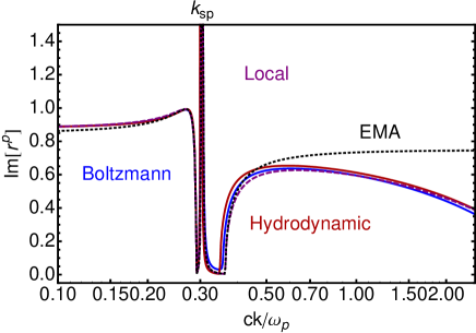
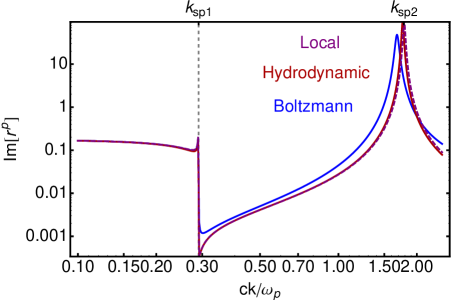
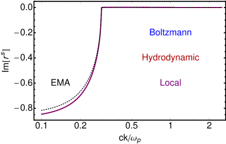
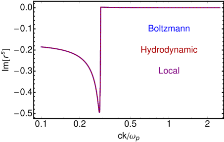
Figure 3: (Color online) Top row: Lateral wave-vector dependence of the imaginary part of the reflection coefficients for p-polarized light for a infinite number of silver/silica bilayers (left panel) and a thin silver layer on top of a silica half-space (right panel). The frequency is fixed to $\omega=0.2\omega_{p}$ and the thickness of the silica and silver layers are $p_{1}=0.2c/\omega_{p}\sim 4.4$nm and $p_{2}=0.1c/\omega_{p}\sim 2.2$nm, respectively (see Fig. 2). Bottom row: Same as the top row but for s-polarized light. In each plot, the different curves correspond to different material models for silver: The nonlocal SCIB model based on the Boltzmann equation (blue solid line), the local Drude model (purple dashed line) and the nonlocal hydrodynamic model (red solid line). For comparisons with the case of the periodic structure, also the predictions of the effective medium approximation (EMA, black dashed) Kidwai12 are depicted.

IV.3 Discussion of the Nonlocal Material Models

The two material models described above, display several analogies but also profound differences Feibelman82 ; Ford84 . If we consider the expressions in Eq.(41c), the residue theorem allows us to show that $\eta^{p}(z)$ can be written as the sum of waves that propagate with wave vectors that are solutions of $K^{2}-\epsilon_{t}(K,\omega)\omega^{2}/c^{2}=0$ and $\epsilon_{t}(K,\omega)=0$. Clearly, these solutions correspond to transverse and longitudinal waves, respectively. This correspondence between the models is, however, only qualitative as the expressions for longitudinal and transverse dielectric functions are quite different. For instance, while the hydrodynamic model only exhibits nonlocal modifications to the longitudinal part of the electromagnetic field, the SCIB predicts nonlocal modifications for both the longitudinal and the transverse part of the field. Probably the most apparent difference between the two models concerns the boundary conditions at the interface. While the SCIB model relies on the symmetries of the Boltzmann equation to determine the behavior of electrons at an interface with dielectric materials, the hydrodynamic description uses the non-locality to implement a finite density of electrons at the interface which removes the discontinuity in the $z$-component of the displacement field.

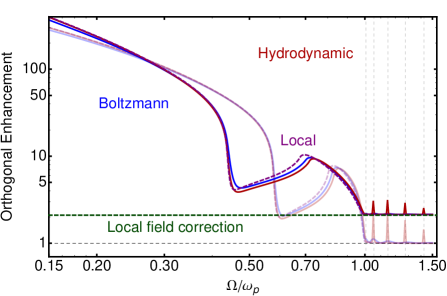
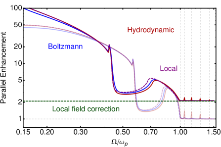
Figure 4: (Color online) Spontaneous emission enhancement factor derived from the orthogonal (left) and parallel (right) components of the scattering Green’s tensor of an infinite sequence of alternating silver and silica layers. The different curves correspond to different material models for silver: The nonlocal SCIB model based on the Boltzmann equation (blue solid line), the local Drude model (purple dashed line) and the nonlocal hydrodynamic model (red solid line). In order to highlight the impact of the local-field corrections, the same computations have been carried out for the same parameters except for replacing silica by vacuum. The results are displayed in the semi-transparent curves. In particular, the incorporation of local-field effects leads to a significant broadening of the plasmon resonance. The gray dashed lines indicate the position of the odd bulk plasmon resonance as give in eq.(60) ($\omega^{\rm B}_{2n+1}$). See the text for details regarding the geometric and material parameters.

Despite these differences, the two non-local models provide qualitatively similar results for the reflection coefficients of the infinitely periodic structures and of a thin silver slab embedded in silica matrix. In Fig. 3 we represent the imaginary part of the corresponding reflection coefficients for the p- and s-polarization. The quantities are plotted as functions of the lateral wave-vector for a fixed frequency ($\omega=0.2\omega_{p}$). We note that for the periodic structure the usual effective medium approach (EMA) in terms of a local dielectric functions Orlov11 ; Chebykin11 provides a good description of the system for sufficiently small wave-vectors (see Fig.3) Kidwai12 . As expected, Kidwai12 the agreement degrades at larger wave-vectors. The plasmon resonance of the periodic structure ($k_{\rm sp}$, see top left panel of Fig. 3) coincides with the surface-plasmon-polariton (SPP) of a silica/metal interface

$$k_{\rm sp}(\omega)=\frac{\omega}{c}\sqrt{\frac{\epsilon(\omega)\epsilon_{\rm D}(\omega)}{\epsilon(\omega)+\epsilon_{\rm D}(\omega)}}\leavevmode\nobreak\ .$$ (58)

The thin single metallic layer exhibits two resonances associated with the symmetric and antisymmetric coupling of the SPPs on the two metal/silica interfaces ($k_{\rm sp1}$ and $k_{\rm sp2}$, see top right panel of Fig. 3) which in other context’s are know as the short-range and the long-range SPP, respectively Berini09 ). In the local description for frequency smaller than $\omega_{p}$ and small thickness the resonances’ positions are approximatly given by

$$k_{\rm sp1}(\omega)\sim\frac{\omega}{c}\sqrt{\epsilon(\omega)}\leavevmode\nobreak\ ,$$ (59a)

$$k_{\rm sp2}(\omega)\sim\sqrt{\left[\frac{2\epsilon(\omega)}{p_{2}\epsilon_{\rm D}(\omega)}\right]^{2}+\frac{\omega^{2}}{c^{2}}\epsilon(\omega)}\leavevmode\nobreak\ .$$ (59b)

which correspond to the values for the symmetric (near the light cone) and anti-symmetric SPPs. The anti-symmetric resonance is much stronger than the symmetric resonance. It is also worth noting that for the anti-symmetric SPP the SCIB gives rise to a value which is different from the value for the local and the hydrodynamic description. For s-polarized radiation, the behavior is much simpler and the nonlocality only slightly affects the reflection coefficients. In all cases, a characteristic abrupt change occurs at the light cone, i.e. for $k\sim\omega\sqrt{\epsilon(\omega)}/c$.

V Results

We now apply the above formalism to study the modified radiation dynamics of an emitter embedded in two distinct structures. The first structure consists of a central cavity silica layer ($D=2c/\omega_{p}$) that is symmetrically sandwiched between infinite sequences of bilayers of silver ($p_{2}=0.1c/\omega_{p}$) and silica ($p_{1}=0.2c/\omega_{p}$) as depicted in Fig. 2. The second structure comprises the same central cavity silica layer that is symmetrically sandwiched between two silver layers with thickness $p_{2}=0.1c/\omega_{p}$ and this composite slab-structure is embedded into two half spaces of silica. The dielectric properties of silica are described via a three-oscillator model Gunde00 and we consider the above-discussed and widely used material models for silver, i.e., the local Drude model, the SCIB model and the hydrodynamic model. All these models employ the same plasma frequency $\omega_{p}=8.89$ eV ($c/\omega_{p}\sim 22$nm) and damping constant $\Gamma=0.018$ eV. Additionally, the SCIB model and the hydrodynamic model use the Fermi velocity $v_{F}=1.39\times 10^{6}$ m/s) of silver Iorsh12 . In both of the above structures, we position an emitter midway in the cavity layer ($d=c/\omega_{p}$) and the radius of the real-cavity model for the local field correction is $R=10^{-2}c/\omega_{p}$.

V.1 Decay Enhancement and Frequency Shift in Infinite Periodic Structure

In Fig. 4 we depict the results of the spontaneous emission enhancement factor for a dipole oriented orthogonal and parallel to the stacking direction of the above-described infinite periodic structure. For comparison, we have also included the results of computations where silica has been replaced by vacuum (or air). As expected, the nonlocal material models lead to a slight blue shift of the main plasmon resonance around $\omega/\omega_{p}=1\sqrt{2}\sim 0.7$ relative to the local Drude model. The decay rates essentially follow the dispersion relation of the surface plasmons coupled across the cavity containing the emitter. From the expressions of the orthogonal and parallel components of the Green’s tensor in eqs.(12b) one deduces that the orthogonal enhancement is associated with the dispersion relation of the anti-symmetric cavity surface plasmon while the behavior of the parallel enhancement can be associated with the dispersion relation of the symmetric cavity surface plasmon Mochan87 ; Haakh13 ; Intravaia05 ; Intravaia07 : The integrals in eqs.(12b) can be approximatively evaluated as the residues for the corresponding cavity plasmon. Upon using dimension less variables $\omega/c\to\omega d/c$ and $k\to kd$ in eqs.(12b), one can infer that the behavior at low frequencies is equivalent to a reduction of the distance between the emitter and the interface explaining the large enhancement of the decay. In this same region ($\omega/\omega_{p}\lesssim 0.2$) the hydrodynamic model gives results very similar to the local description while the SCIB model produces slightly a different prediction (more pronounced when we use silica instead of vacuum for the dielectric layer). At frequencies higher than the plasma frequency, we observe additional resonances for the nonlocal materials models. These resonances corresponds to the excitation of bulk plasmons which are known to appear in nonlocal descriptions of the metal beyond the plasma frequency Mochan87 . It is worth noting that while these bulk plasmon resonances occur at roughly the same positions for the SCIB and the hydrodynamic model (a shift appears at large frequencies) they are much less pronounced and wider for the SCIB model (see Fig.5). Approximately, the bulk plasmon resonances are given by

$$\omega^{\rm B}_{n}\approx\sqrt{\omega_{p}^{2}+\left(n\frac{\beta\pi}{p_{2}}\right)^{2}}.$$ (60)

In the hydrodynamic description only the odd frequencies couple to the external radiation Mochan87 while the even resonances are almost decoupled from the external field and can be excited only minimally (see Fig.5). We observe a similar behavior for the SCIB model with the exception of the lowest bulk plasmon frequency $\omega^{\rm B}_{1}$: In the hydrodynamic model this resonance lies in a band gap which forbids any propagation Mochan87 . The situation is different for the model based on the Boltzmann equation, where we clearly observe a resonance at $\omega^{\rm B}_{1}$.

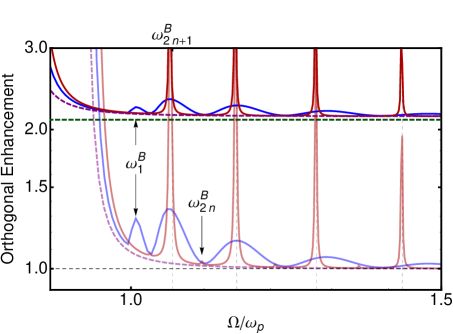
Figure 5: (Color online) Bulk plasmon resonances in the orthogonal enhancement of the spontaneous decay of an emitter located in a cavity formed by two thin metallic layers. The position and behavior of these resonances is similar in all configurations considered in this work. The different curves correspond to different material models for silver: The local Drude model (purple dashed line), the nonlocal hydrodynamic model (red solid line) and the SCIB model based on the Boltzmann equation (blue solid line). See the text for details regarding the geometric and material parameters. In order to highlight the impact of the local-field corrections, the same computations have been carried out for the same parameters except for replacing silica by vacuum. The results are depicted in the semi-transparent curves.

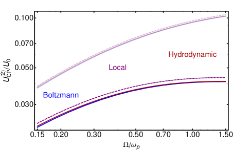
Figure 6: (Color online) Geometric frequency shift for an emitter in a silica nano-cavity sandwiched between infinite sequences of alternating silver and silica layers. The parameters and the models are the same as those used for describing the spontaneous decay (see main text). The values are normalized to $U_{0}=-\hbar\omega_{p}(\alpha_{g}\omega_{p}^{3}/c^{3})(2\pi\epsilon_{0})^{-1}$ and depicted as a functions of the emitter’s transition frequency. The different curves correspond to different material models for silver: The local Drude model (purple dashed line), the nonlocal hydrodynamic model (red solid line) and the SCIB model based on the Boltzmann equation (blue solid line). See the text for details regarding the geometric and material parameters. In order to highlight the impact of the local-field corrections, the same computations have been carried out for the same parameters except for replacing silica by vacuum. The results are depicted in the semi-transparent curves. The local-field corrections significantly reduce the magnitude of these geometry-induced shifts relative to vacuum.

The differences between the nonlocal models are directly connected to the different ways the wave vector (non-locality) and dissipation enter in eqs.(42) and (43) with respect to eqs.(46) and, clearly, also to the different boundary conditions discussed in section IV. Therefore, experimental studies on the spontaneous emission enhancement in such systems for frequencies above the plasma frequency may be able to probe the nature of the plasmonic material.

Upon comparing the results for vacuum with those of silica as the dielectric material, the offset originating from the local-field corrections and the red-shift of the curves as well as of the SPP resonance is clearly visible. Again, this (expected) behavior can be understood in connection with the dispersion relation of the symmetric and anti-symmetric cavity surface plasmons which are expected to red-shift in presence of the dielectrics. Furthermore, the local-field corrections lead to a rather significant broadening of the main plasmon resonance characteristics. Conversely, the positions of the bulk plasmon resonances are not affected by the local field correction and there hardly is any additional broadening for both models. Instead, we observe a reduction in the peak hight.

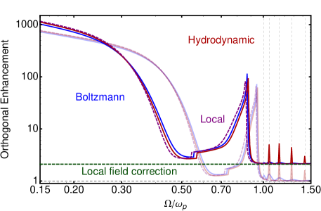
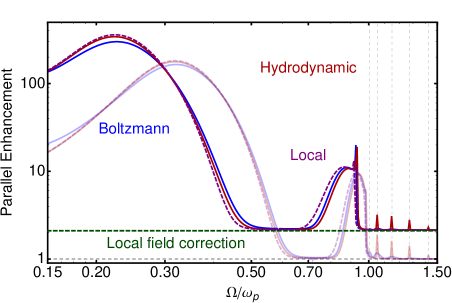
Figure 7: (Color online) Spontaneous emission enhancement factor derived from the orthogonal (left) and parallel (right) components of the scattering Green’s tensor of composite slab structure consisting of a central silica layer sandwiched between two silver layers and completely embedded in silica. The emitter is located in the center of central silica layer. The different curves correspond to different material models for silver: The nonlocal SCIB model based on the Boltzmann equation (blue solid line), the local Drude model (purple dashed line) and the nonlocal hydrodynamic model (purple solid line). In order to highlight the impact of the local-field corrections, the same computations have been carried out for the same parameters except for replacing silica by vacuum. The results are displayed in the semi-transparent curves. The incorporation of local-field effects leads to a significant broadening of the plasmon resonance. The gray dashed lines indicate the position of the odd bulk plasmon resonance as give in eq.(60) ($\omega^{\rm B}_{2n+1}$). See the text for details regarding the geometric and material parameters.

In addition, in Fig. 6 we display the results for the geometrical frequency shift experienced by the emitter in the above-discussed infinite structure. Owing to the fact that this shift results from an integration over imaginary frequencies (c.f. Eq. (17)), no characteristic features resulting from plasmon resonances are visible and the results for the local Drude model and the nonlocal models are very similar and this is in agreement with previous works Esquivel03 ; Esquivel04 ; Roman-Velazquez04 ; Esquivel-Sirvent05 ; Svetovoy05 . Also, the differences between the SCIB and the hydrodynamic description are less prominent and both models essentially provide the same result. Nevertheless, the local-field corrected computations for silica yield geometry-induced shifts that are significantly reduced with respect to the computations for vacuum. This is the result of an effective screening provided by the dielectric material.

V.2 Decay Enhancement for a Finite Slab Structure

In Fig. 7, we display the spontaneous emission enhancement factor for a dipole oriented orthogonal and parallel to the stacking direction of the above-described slab structure. For comparison, we have included the results of computations where silica has been replaced by vacuum (or air). Also in this case the enhancement factor shows the features described above. As before, we observe the characteristic blue-shift of the main plasmon resonance between the local Drude description and the nonlocal descriptions for the plasmonic layers as well as the occurence of bulk plasmon resonances for frequencies above the plasma frequency, strong resonances for the hydrodynamic model and weak resonances for the SCIB model. Similarly, the comparison of the local-field corrected computations for silica with the computations for vacuum reveal that in the case of silica the main plasmon resonance is much broader and the bulk plasmon resonance peaks are suppressed. However, we would like to note that the enhancement values generally are much larger than for the infinite system discussed above. This is for our specific choice of geometric parameters the resonance in the reflection coefficient for the thin slab are much stronger as compared to the infinitely layered system (see Fig. 3). Finally, in the composite silica-silver slab system for frequencies $\omega/\omega_{p}\lesssim 0.2$, we observe again differences between the emission enhancements related to the nonlocal SCIB description and to the hydrodynamic model. This occurs for both dipole’s orientation whereas for these frequencies, the results of the hydrodynamic model agrees rather well with those of the Drude model. In this case we can connect this behavior with the features of the p-reflection coefficient in Fig. 3.

In summary, we have developed a comprehensive framework for computing decay enhancements and level shifts for emitters embedded in arbitrary layered structures. This framework is capable of including local-field corrections in (weakly absorbing) dielectric systems and can treat the nonlocal optical properties of metals. All these features influence the emitters’s dynamic in a non-additive way, which is also amplified by the relative complexity of the surrounding structure. Nevertheless we were able to show that the local-field corrections generally introduce an offset in the spontaneous decay rates and lead to broadening of plasmon resonances below the plasma frequency. In addition, local-field corrections effectively reduce geometry-induced level shifts. Furthermore, we have found that the differences between the different material models for metals can be analyzed either by changing the dielectric material between the metal layers or by carefully inspecting the decay rates for frequencies above the plasma frequency. While this may be unrealizable for silver-based structures, we would like to point out that recent advances in highly-doped semiconductors place their plasma frequency in the near infrared Sadofev13 , thus rendering such investigations experimentally feasible.

VI Acknowledgments

We acknowledge support by the Deutsche Forschungsgemeinschaft (DFG) through the sub-projects B10 within the Collaborative Research Center (CRC) 951 Hybrid Inorganic/Organic Systems for Opto-Electronics (HIOS). FI further acknowledges financial support from the European Union Marie Curie People program through the Career Integration Grant No. 631571 and through the German-Israeli Project Cooperation (DIP) project “Quantum Phenomena in Hybrid Systems: Interfacing Engineered Materials and Nanostructures with Atomic Systems”.

References

- (1) I. Iorsh, A. Poddubny, A. Orlov, P. Belov, and Y. S. Kivshar, Phys. Lett. A 376, 185 (2012).
- (2) O. Kidwai, S. V. Zhukovsky, and J. E. Sipe, Phys. Rev. A 85, 053842 (2012).
- (3) A. Poddubny, I. Iorsh, P. Belov, and Y. Kivshar, Nat Photon 7, 948 (2013).
- (4) P. A. Belov and Y. Hao, Phys. Rev. B 73, 113110 (2006).
- (5) G. A. Wurtz et al., Nat Nano 6, 107 (2011).
- (6) C. L. Cortes, W. Newman, S. Molesky, and Z. Jacob, J. Optics 14, 063001 (2012).
- (7) W. Yan, M. Wubs, and N. A. Mortensen, Phys. Rev. B 86, 205429 (2012).
- (8) U. Hoeppe, C. Wolff, J. Küchenmeister, J. Niegemann, M. Drescher, H. Benner, and K. Busch, Phys. Rev. Lett. 108, 043603 (2012).
- (9) J. M. Wylie and J. E. Sipe, Phys. Rev. A 30, 1185 (1984).
- (10) L. Novotny and B. Hecht, Principles of Nano-Optics (Cambridge University Press, Cambridge, 2012)
- (11) J. Jackson, Classical Electrodynamics (John Wiley and Sons Inc., New York, 1975).
- (12) R. J. Glauber and M. Lewenstein, Phys. Rev. A 43, 467 (1991).
- (13) P. de Vries and A. Lagendijk, Phys. Rev. Lett. 81, 1381 (1998).
- (14) S. Scheel, L. Knöll, D.-G. Welsch, and S. M. Barnett, Phys. Rev. A 60, 1590 (1999).
- (15) S. Scheel, L. Knöll, and D.-G. Welsch, Phys. Rev. A 60, 4094 (1999).
- (16) M. Fleischhauer, Phys. Rev. A 60, 2534 (1999).
- (17) M. S. Tomas, Phys. Rev. A 63, 053811 (2001).
- (18) H. T. Dung, S. Y. Buhmann, and D.-G. Welsch, Phys. Rev. A 74, 023803 (2006).
- (19) J. M. Wylie and J. E. Sipe, Phys. Rev. A 32, 2030 (1985).
- (20) M. S. Tomas, Phys. Rev. A 51, 2545 (1995).
- (21) A. Sambale, S. Y. Buhmann, D.-G. Welsch, and M.-S. Tomas, Phys. Rev. A 75, 042109 (2007).
- (22) S. Scheel and S. Y. Buhmann, Acta Physica Slovaca 58, 675 (2008).
- (23) W. L. Mochán, M. del Castillo-Mussot, and R. G. Barrera, Phys. Rev. B 35, 1088 (1987).
- (24) F. Intravaia, C. Henkel, and M. Antezza, in Casimir Physics, Vol. 834 of Lecture Notes in Physics, edited by D. Dalvit, P. Milonni, D. Roberts, and F. da Rosa (Springer, Berlin / Heidelberg, 2011), pp. 345–391.
- (25) H. R. Haakh and F. Intravaia, Phys. Rev. A 88, 052503 (2013).
- (26) K. Busch, G. von Freymann, S. Linden, S.F. Mingaleev, L. Tkeshelashvili, and M. Wegener, Phys. Rep. 444, 101 (2007).
- (27) P. Yeh, A. Yariv, and C.-S. Hong, J. Opt. Soc. Am. 67, 423 (1977).
- (28) A. Yariv and P. Yeh, Optical Waves in Crystals (John Wiley & Sons, New York, 1983)
- (29) P. J. Feibelman, Prog. Surf Sci. 12, 287 (1982).
- (30) G. W. Ford and W. H. Weber, Phys. Rep. 113, 195 (1984).
- (31) K. L. Kliewer and R. Fuchs, Phys. Rev. 172, 607 (1968).
- (32) W. E. Jones, K. L. Kliewer, and R. Fuchs, Phys. Rev. 178, 1201 (1969).
- (33) R. Fuchs and K. L. Kliewer, Phys. Rev. 185, 905 (1969).
- (34) B. Horovitz and C. Henkel, Europhys. Lett. 97, 57010 (2012).
- (35) J. Lindhard, Kgl. Danske Videnskab. Selskab Mat.-Fys. Medd. 28, (1954).
- (36) F. Bloch, Helv. Phys. Acta 7, (1934).
- (37) G. Barton, Rep. Prog. Phys. 42, 963 (1979).
- (38) S. Raza, G. Toscano, A.-P. Jauho, M. Wubs, and N. A. Mortensen, Phys. Rev. B 84, 121412 (2011).
- (39) P. Berini, Adv. Opt. Photonics 1, 484 (2009)
- (40) R. Ruppin and R. Engleman, Phys. Rev. Lett. 53, 1688 (1984)
- (41) A. V. Chebykin, A. A. Orlov, A. V. Vozianova, S. I. Maslovski, Y. S. Kivshar, and P. A. Belov, Phys. Rev. B 84, 115438 (2011).
- (42) A. A. Orlov, P. M. Voroshilov, P. A. Belov, and Y. S. Kivshar, Phys. Rev. B 84, 045424 (2011).
- (43) M. K. Gunde, Physica B 292, 286 (2000).
- (44) F. Intravaia and A. Lambrecht, Phys. Rev. Lett. 94, 110404 (2005).
- (45) F. Intravaia, C. Henkel, and A. Lambrecht, Phys. Rev. A 76, 033820 (2007).
- (46) R. Esquivel, C. Villarreal, and W. L. Mochan, Phys. Rev. A 68, 052103 (2003). See also the Erratum: Phys. Rev. A 71, 029904 (2005).
- (47) R. Esquivel and V. B. Svetovoy, Phys. Rev. A 69, 062102 (2004).
- (48) C. E. Roman-Velazquez, C. Noguez, C. Villarreal, and R. Esquivel-Sirvent, Phys. Rev. A 69, 042109 (2004).
- (49) R. Esquivel-Sirvent and V. B. Svetovoy, Phys. Rev. B 72, 045443 (2005).
- (50) V. B. Svetovoy and R. Esquivel, Phys. Rev. E 72, 036113 (2005).
- (51) S. Sadofev, S. Kalusniak, P. Schäfer, and F. Henneberger, Appl. Phys. Lett. 102, 181905 (2013)