New results for electromagnetic quasinormal and quasibound modes of Kerr black holes

Abstract

The perturbations of the Kerr metric and the miracle of their exact solutions play a critical role in the comparison of predictions of general relativity with astrophysical observations of compact massive objects. The differential equations governing the late-time ring-down of the perturbations of the Kerr metric, the Teukolsky Angular Equation and the Teukolsky Radial Equation, can be solved analytically in terms of confluent Heun functions. In this article, we solve numerically the spectral system formed by those exact solutions and we obtain the electromagnetic (EM) spectra of the Kerr black hole.

Because of the novel direct way of imposing the boundary conditions, one is able to discern three different types of spectra: the well-known quasinormal modes (QNM), the symmetric with respect to the real axis quasibound modes (QBM) and a spurious spectrum who is radially unstable. This approach allows clearer justification of the term ‘‘spurious’’ spectrum, which may be important considering the recent interest in the spectra of the electromagnetic counterparts of events producing gravitational waves.

Keywords quasinormal modes, Kerr metric, QNM, quasibound modes, Teukolsky radial equation, Teukolsky angular equation, confluent Heun function

1 Quasi-normal modes of black holes

During the long history of the study of the quasinormal modes (QNMs) of a black hole (BH) (Regge & Wheeler (1957); Zerilli (1970); Vishveshwara (1970),
Bardeen et al. (1972),Teukolsky (1972, 1973, 2014), Press & Teukolsky (1973); Teukolsky & Press (1974); Chandrasekhar (1975, 1976a, 1976b), Chandrasekhar (1983), Chandrasekhar & Detweiler (1975); Detweiler (1976, 1980),Leaver (1985, 1986); Andersson (1992),
Berti et al. (2003, 2009), Berti (2004); Fiziev (2006); Ferrari & Gualtieri (2007), Fiziev (2009, 2010a),
Hod & Hod (2010),Hod (2011), Konoplya & Zhidenko (2011)), the case of electromagnetic (EM) perturbations has been often ignored in favor to the gravitational one. It is considered that the gravitational output should be significantly more luminous than the EM one (Schnittman (2011)), which combined with the strong absorption of the EM spectrum by the interstellar medium, makes the detection very difficult at the predicted low frequencies for the electromagnetic QNMs. On the other hand, the gravitational waves (GW) interact very weakly with matter and thus they can travel big distances without getting absorbed or scattered, i.e. without obscuring the signature of the body that emitted them. It is, therefore, reasonable to expect that the GW should be much better suited for studying the central engines of astrophysical events, such as gamma-ray bursts (GRBs).

The lack of GW detection from both LIGO and VIRGO (LIGO & VIRGO (2010a, 2011); Abadie et al. (2011, 2012, 2013, 2014) ), however, forced the introduction of the so-called multimessenger approach. With it, one can use the EM counterpart of the GW emission to gain more complete picture on the event and to improve the localization of the source and the sensitivity of the analysis of the GW data Coward et al. (2011); Schnittman (2011); LIGO & VIRGO (2012); Christensen (2011); Bogdanovic et al. (2011),
Moesta et al. (2011).

In the case of short GRBs, the negative results may be explained by a GRB-generating process which in good approximation preserves the spherical symmetry of the central engine and thus admits only significant dipole radiation (EM waves) and no quadrupole one (GW waves). It can also be due to the unknown model-dependent ratio between EM and GW emission in more traditional processes. In the absence of GW detection, studying the characteristic EM spectrum of the object is the best path to understand the GRB central engine.

The discrete spectrum of complex frequencies called QNMs describe only the linearized perturbations of the metric. For this reason, they cannot describe the dynamics of the process during the early, highly intensive stage of the event, when the linearized theory is not applicable. In EM observations, however, we ‘‘see’’ only the tails of the event, being far from them. Furthermore, it is known from full numerical simulations that the QNMs dominate the late-time evolution of the object’s response to perturbations (Berti et al. (2003), Jaramillo et al. (2012)).

The QNMs correspond to particular boundary conditions characteristic of the object in question. In the case of BHs, the no-hair theorem states that they should depend only on the parameters of the metric, which means that measuring those frequencies observationally can be used to test the nature of the object – a black hole or other compact massive object like super-spinars (naked singularities), neutron stars, black hole mimickers etc. (Berti et al. (2006); Chirenti & Rezzolla (2007, 2008); Schutz et al. (2011); Pani et al. (2009); Staicova & Fiziev (2010)). It also can constrain additionally the no-hair theorem, which has recently been called into question for the case of black holes formed as a result of the collapse of rotating neutron stars Lyutikov & McKinney (2011).

An interesting possibility is to find a way to use the damping times of the EM quasinormal modes for comparison with observations. While the frequencies can be distorted by interaction with the surrounding matter, their damping times should be related to the variability-scale of the event. Recent simulations of jet propagation imply that the short-scale variability of the light-curve is due to the central engine and not to the interaction of the jet with the surrounding medium (see Gao et al. (2011)). Such studies could be particularly interesting in the case of the central engines of GRBs, where numerical simulations although capable of describing some of the features of the GRBs light curves (for a review on GRBs, see Zhang (2011)), still struggle to explain the extended duration and characteristic time-variability (for a novel model working in this direction see for example Rezzolla & Kumar (2014)).

Existing models of GRB central engine include a compact massive object (black hole or a milli-second magnetar) and extreme magnetic field ($\sim 10^{15}G$ ) to accelerate and collimate the matter. Such central engine can be studied approximately by the linearized perturbations of the Kerr black hole. The spectrum of such perturbation do not depend on the origin of the perturbation, but only on the parameters of the compact massive object (mass and spin). In the idealized EM case, the perturbation is described by free EM waves in vacuum. While the astrophysical black holes are thought to be not charged, they are immersed into EM waves with different energy and origin. The black hole response to such EM perturbations in linear approximation will be, then, the QNM spectrum defined by the appropriate boundary conditions .

The choice of the rotating Kerr black hole, instead of the simpler Schwarzschild case, is due to the fact that rotation is critical in known energy extraction processes (for example resonant amplification or the Blandford-Znajek process Teukolsky & Press (1974); Hod & Hod (2010); Hod (2011)). Available observationally measured rotations of astrophysical compact massive objects show that there are many cases of near extremal values (for example the rotation rates of two astrophysical black holes, Sw J1644+57 with $a=0.9M$ and Sw J2058+05 with $a=0.99M$ Lei & Zhang (2011)).

To obtain the QNM spectra, one needs to solve two second-order linear differential equations: the Teukolsky radial equation (TRE) and the Teukolsky angular equation (TAE) and to impose on them specific boundary conditions (Chandrasekhar & Detweiler (1975); Chandrasekhar (1983)). Until recently, solving those equations analytically was considered impossible in terms of known functions, so approximations with more simple wave functions were used instead. The resulting system of spectral equations – a connected problem with two complex spectral parameters: the frequency $\omega$ and the separation constant $E$ – has been solved using different methods (Berti (2004); Ferrari & Gualtieri (2007); Berti et al. (2009); Konoplya & Zhidenko (2011)) with notably the most often used being the method of continued fractions adapted by Leaver from the problem of the hydrogen molecule ion in quantum mechanics Leaver (1985, 1986). This method, while being successful in obtaining the QNMs spectra, has some specific numerical problems, for example in calculation of purely imaginary modes (Leaver (1986), p.8) and also it doesn’t account for the branch cuts in the exact solutions.

The analytical solutions of the TRE and the TAE can be written in terms of the confluent Heun function (for $a\neq M$) as done for the first time in Fiziev (2006, 2010a, 2010b, 2009). Those functions are the unique local Frobenius solutions of a second-order linear ordinary differential equation of the Fucsian type Heun (1889); Decarreau et al. (1978a, b); Slavyanov & Lay (2000); Ronveaux (1995) with 2 regular singularities ($z=0,1$) and one irregular ($z=\infty$) and they are denoted as: $\text{HeunC}(\alpha,\beta,\gamma,\delta,\eta,z)$ (normalized to $\text{HeunC}(\alpha,\beta,\gamma,\delta,\eta,0)=1$). The confluent Heun function as implemented in the software package maple was used successfully in our previous works Fiziev (2006); Staicova & Fiziev (2010); Fiziev & Staicova (2011a, 2012). The advantage of using the analytical solutions is that one can impose the boundary conditions on them directly (see Fiziev (2006); Staicova & Fiziev (2010)) and thus to be able to control all the details of the physics of the problem. It is thought that the Teukolsky-Starobinsky identities stem from the fact that both the TRE and TAE can be solved in terms of the confluent Heun function Teukolsky (2014).

In a series of articles, we developed a method for solving numerically two-dimensional systems featuring the Heun functions (the two-dimensional generalization of the Müller method described in Fiziev & Staicova (2011b)) and we used it successfully in the case of gravitational perturbation ($s=-2$) of the Schwarzschild metric Fiziev & Staicova (2012). Besides repeating with high precision the already known results, we used the epsilon-method (see below) to study the branch cuts in the spectral problem and to show that the $9^{th}$ mode for $s=-2$ is not purely imaginary, and thus cannot be algebraically special. Analysis of the potentials of the Regge-Wheeler equation (RWE) and the Zerilli equation (ZRE) showed that its properties are due to the existence of a branch cut on the imaginary axis for this mode Maassen van den Brink (2000); Leung et al. (2003). This result is directly obtainable from the actual solutions of the RWE and ZRE in terms of the confluent Heun functions.

In this article, we continue the exploration of the application of the confluent Heun functions by studying the QNMs of the Kerr BH. Previous results, obtained in Staicova & Fiziev (2011) showed that using the confluent Heun function one can obtain the QNMs to a very good precision for the well-known lower modes. In the current work we are able to obtain the QNMs for a wide range of modes and rotational parameters and we show that there is a very good agreement between our results and those obtained with other methods. Additionally, we study the numerical stability of the solutions with respect to the position of the radial variable in the complex plane. Such a study cannot be carried out with the continued fractions method, where the radial variable does not enter explicitly into the equations.

Taking advantage of direct way of imposing the boundary conditions on the system, one obtains not only the QNM spectrum but also the quasibound (quasiresonant) one (QBM). The QBMs form a discrete spectrum of frequencies with negative imaginary parts, obtained by imposing boundary conditions inverse to those of the QNMs. Those boundary conditions can correspond to time-inversion and are expected to be part of the solution due to its symmetries. They can also be considered as unstable bounded waves reflected by the horizon and infinity. An example of the study of the quasibound states in the case of massive vector propagating on the Schwarzschild space-time can be found in Rosa & Dolan (2012). Finally, we obtain an additional spectrum which is found to be spurious with respect to the so-defined spectral problem.

2 The Teukolsky angular equations

In Chandrasekhar’s notation, the Teukolsky Master Equation (Teukolsky & Press (1974)), for $|s|=1$, is separable under the substitution $\Psi\!=\!e^{i(\omega t\!+\!m\phi)}S(\theta)R(r)$, where $m=0,\pm 1,\pm 2$ for integer spins and $\omega$ is the complex frequency. Due to the choice of this form of $\Psi$, the sign of $\omega$ differs from the one Teukolsky used, and the stability condition, guaranteeing that the perturbations will damp with time reads $\Im(\omega)>0$.

The TAE for EM perturbations ($s=-1$) has 16 classes of exact solutions $S(\theta)$ in terms of the confluent Heun functions (for full details see Fiziev (2010a)). To fix the spectrum approximately, one requires an additional regularity condition for the angular part of the perturbation, which means that if we choose one solution, $S_{1}(\theta)$, regular around the one pole of the sphere ($\theta=0$) and another, $S_{2}(\theta)$, which is regular around the other pole ($\theta=\pi$), then in order to ensure a simultaneous regularity, the Wronskian of the two solutions should become equal to zero, $W[S_{1}(\theta),S_{2}(\theta)]=0$. This gives us one of the equations for the two-dimensional spectral system defining QNM.

In Fiziev (2010a), there are four pairs of Wronskians, each pair being valid in a sector of the plane $\{s,m\}$. The Wronskians we used to obtain the spectra are:

$$W[S_{1},S_{2}]=\frac{\text{HeunC}^{\prime}(\alpha_{1},\beta_{1},\gamma_{1},\delta_{1},\eta_{1},\left(\cos\left(\pi/6\right)\right)^{2})}{\text{HeunC}(\alpha_{1},\beta_{1},\gamma_{1},\delta_{1},\eta_{1},\left(\cos\left(\pi/6\right)\right)^{2})}+$$

$$\frac{\text{HeunC}^{\prime}(\alpha_{2},\beta_{2},\gamma_{2},\delta_{2},\eta_{2},\left(\sin\left(\pi/6\right)\right)^{2})}{\text{HeunC}(\alpha_{2},\beta_{2},\gamma_{2},\delta_{2},\eta_{2},\left(\sin\left(\pi/6\right)\right)^{2})}+p=0$$ (1)

where the derivatives are with respect to $z$ and the values of the parameters for the two confluent Heun functions for each $m$ are as follows:

For the case $m=0$: $\alpha_{1}=4\,a\omega,\beta_{1}=1,\gamma_{1}=-1,\delta_{1}=4\,a\omega,\eta_{1}=1/2-E-2\,a\omega-{a}^{2}{\omega}^{2}$ and

$\alpha_{2}=-4\,a\omega,\beta_{2}=1,\gamma_{2}=1,\delta_{2}=-4\,a\omega,\eta_{2}=,1/2-E+2\,a\omega-{a}^{2}{\omega}^{2}$, $p=\frac{1}{\left(\sin\left(\pi/6\right)\right)^{2}}$

For the case $m=1$: $\alpha_{1}=-4\,a\omega,\beta_{1}=2,\gamma_{1}=0,\delta_{1}=4\,a\omega,\eta_{1}=1-E-2\,a\omega-{a}^{2}{\omega}^{2}$ and

$\alpha_{2}=-4\,a\omega,\beta_{2}=0,\gamma_{2}=2,\delta_{2}=-4\,a\omega,,\eta_{2}=1-E+2\,a\omega-{a}^{2}{\omega}^{2}$ and $p=-4\,a\omega$

For the case m=2: $\alpha_{1}=-4\,a\omega,\beta_{1}=3,\gamma_{1}=-1,\delta_{1}=4\,a\omega,\eta_{1}=5/2-E-2\,a\omega-{a}^{2}{\omega}^{2}$ and

$\alpha_{2}=-4\,a\omega,\beta_{2}=1,\gamma_{2}=-3,\delta_{2}=-4\,a\omega,\eta_{2}=5/2-E+2\,a\omega-{a}^{2}{\omega}^{2}$ and $p=8-4a\omega.$

where we use $\theta=\pi/3$ (the QNMs should be independent of the choice of $\theta$ in the spectral conditions).

This form of the Wronskians, different from the one in Fiziev (2010a), is chosen to improve the numerical convergence of the root-finding algorithm.

3 The Teukolsky radial equation

The TRE differential equation is of the confluent Heun type, with $r=r_{\pm}$ regular singular points and $r=\infty$ – irregular one. As it was noted in Staicova & Fiziev (2010), the point $r=0,\theta=\pi/2$ is not a singularity for this equation. The solutions of the TRE for $r>r_{+}$, are :

$$R(r)\!=\!C_{1}R_{1}(r)+C_{2}R_{2}(r),\text{for}$$ (2)

$$R_{1}(r)\!=\!e^{\frac{\alpha\,z}{2}}(r\!-\!r_{+})^{\frac{\beta\!+\!1}{2}}(r\!-\!r_{-})^{\frac{\gamma\!+\!1}{2}}\text{HeunC}(\alpha,\beta,\gamma,\delta,\eta,z)\!$$

$$R_{2}(r)\!=R_{1}(r)(\beta\to-\beta)$$

where $z=-\frac{r-r_{+}}{r_{+}-r_{-}}$ and the parameters are:

$$\alpha \!=\!-2\,i\left({\it r_{{}_{+}}}\!-\!{\it r_{{}_{-}}}\right)\omega,\beta\!=\!-\!{\frac{2\,i(\omega\,({a}^{2}+{{\it r_{{}_{+}}}}^{2})\!+\!am)}{{\it r_{{}_{+}}}\!-\!{\it r_{{}_{-}}}}}\!-\!1,$$

$$\gamma \!=\!{\frac{2\,i(\omega\,({a}^{2}\!+\!{{\it r_{{}_{-}}}}^{2})\!+\!am)}{{\it r_{{}_{+}}}\!-\!{\it r_{{}_{-}}}}}\!-\!1,\delta\!=\!2i\!\left({\it r_{{}_{-}}}\!-\!{\it r_{{}_{+}}}\right)\!\left(\omega\!-\!i\left({\it r_{{}_{-}}}\!+\!{\it r_{{}_{+}}}\right)\omega^{2}\right)\!$$

$$\eta =\!\frac{1}{2}\frac{1}{{\left({\it r_{{}_{+}}}\!-\!{\it r_{{}_{-}}}\right)^{2}}}\Big{[}4{\omega}^{2}{{\it r_{{}_{+}}}}^{4}\!+\!4\left(i\omega\!-\!2{\omega}^{2}{\it r_{{}_{-}}}\right){{\it r_{{}_{+}}}}^{3}\!+\!(1\!-\!4a\omega\,m\!-$$

$$\!2{\omega}^{2}{a}^{2}\!-\!2E)\left({{\it r_{{}_{+}}}}^{2}\!+\!{{\it r_{{}_{-}}}}^{2}\right)\!+4\left(i\omega\,{\it r_{{}_{-}}}\!-\!2i\omega\,{\it r_{{}_{+}}}\!+\!E\!-\!{\omega}^{2}{a}^{2}\!-\!\frac{1}{2}\right)\times$$

$${\it r_{{}_{-}}}\,{\it r_{{}_{+}}}\!-4{a}^{2}\left(m\!+\!\omega\,a\right)^{2}\Big{]}.$$

Here the general solution is constructed following the theory of the Fucsian equations. Accounting for the symmetries of the confluent Heun function, the solutions (2) coincide with those in Fiziev (2010a)(with $\omega\!\to\!-\!\omega$).

The TRE has 3 singular points $r_{-},r_{+},\infty$ and in order to fix the spectrum, one needs to impose specific boundary conditions on two of those singularities (i.e. to solve the central two-point connection problem Slavyanov & Lay (2000)). Different boundary conditions on different pairs of singular points will mean different physics of the problem. The QNM spectrum is obtained trough the so called black hole boundary conditions (BHBC) – waves going simultaneously into the event horizon ($r_{+}$) and into infinity – following the same reasoning as in Staicova & Fiziev (2010) where additional details can be found. Then, the BHBC read:

1. BHBC on the KBH event horizon $r_{+}$.

   For $r\to r_{+}$, from $r(t)=r_{+}+e^{\frac{-\Re(\omega)t+const}{\Im(n_{1,2})}}\to r_{+}$, where $n_{1,2}$ are the powers of the factor $(r-r_{+})^{n_{1,2}}$ in $R_{1,2}$. Thus for $m=0$, the only valid solution in the whole interval $\Re(\omega)\in(-\infty,\infty)$ is $R_{2}$, while for $m\neq 0$, the solution $R_{2}$ is valid for $\Re(\omega)\not\in(-\frac{ma}{2Mr_{+}},0)$, in the rest of the interval one needs to use $R_{1}$ to describe ingoing waves. When this condition is not fulfilled, the spectrum corresponds to waves going out of the horizon – a white hole case.

2. BHBC at infinity.

   At $r\to\infty$, the solution is a linear combination of an ingoing ($R_{\leftarrow}$) and an outgoing ($R_{\rightarrow}$) wave: $R=C_{\leftarrow}\,R_{\leftarrow}+C_{\rightarrow}\,R_{\rightarrow},$ where $C_{\leftarrow}$, $C_{\rightarrow}$ are unknown constants and $R_{\leftarrow},R_{\rightarrow}$ are found using the asymptotics of the confluent Heun function as in Slavyanov & Lay (2000); Fiziev (2010a).

   To ensure only outgoing waves at infinity, one needs to have $C_{\leftarrow}=0$.

   To achieve this, one first finds the direction of the steepest descent in the complex plane $\mathbb{C}_{r}$ for which $\lim\limits_{r\to\infty}\frac{R_{\rightarrow}}{R_{\leftarrow}}=r^{-4i\,\omega\,M+2}e^{-2i\omega\,r}=0$ tends to zero the most quickly: $\sin(\arg(\omega)\!+\!\arg(r))\!=\!-\!1$. This gives us the relation $r=\mid\!r\!\mid e^{3/2i\pi-i\,\arg(\omega)}$ (Fiziev (2006)), between $\omega$ and $r$, which is exact only if one uses the first term of the asymptotic series for the confluent Heun function (i.e. $\text{HeunC}\sim 1$).

   To completely specify the spectrum $\{\omega_{n,m},E_{n,m}\}$, for $R=R_{2}$ ($R_{1}$ is analogous), it is enough to solve:

   $$C_{\leftarrow}\!=\!r^{2\!+\!i\,\omega\!+\!\frac{2i\,m\,a\!+\!i\,\omega}{r_{+}\!-\!r_{-}}}\text{HeunC}(\alpha,\!\!-\!\beta,\gamma,\delta,\eta,z)\!=\!0,$$ (3)

The inverse boundary conditions, namely waves outgoing from the horizon and outgoing from infinity ($\lim\limits_{r\to\infty}\frac{R_{\leftarrow}}{R_{\rightarrow}}=0)$ give the QBM spectrum. Although the QBM frequencies are considered unphysical, because they lead to non-damping waves and thus to a black hole bomb, mathematically the differential system describes those states on equal footing as the QNMs.

4 The branch cuts of the radial solution

Equation (3) relies on the direction of the steepest descent defined by the phase condition $\sin(\arg(\omega)+\arg(r))\lessgtr 0$ (upper sign for QNMs, lower – for QBMs). This approximate direction was chosen ignoring the higher terms in the asymptotic expansion of the solution around the infinity point. Therefore, one can expect that the true path in the complex plane may not be a straight line but a curve. In principle, the spectrum should not depend on this curve as long as $r$ stays in the sector of the complex plane where $\lim\limits_{r\to\infty}\frac{R_{\rightarrow}}{R_{\leftarrow}}=0$ for QNM (or the inverse for the QBM).

Complications may arise due to the appearance of branch cuts (BC) in the confluent Heun function. In this numerical realization, as a branch cut is chosen the semi-infinite interval $z\in(1,\infty)$ on the real axis.

Because of the phase condition, the branch cuts in the complex $r$-plane, appear also in the complex $\omega$-plane. In order to localize those branch cuts, we utilize the $\epsilon$-method (Fiziev & Staicova (2011a, 2012)) – we add a small parameter $\epsilon<<1$ to the phase condition $\pi<\arg(r)\!+\!\arg(\omega)+\epsilon\!<2\pi$ (for QNMs), thus effectively moving $r=|r|e^{i\arg(r)}$ in the complex plane.

Then the observed branch cuts are as follow:

1. For $r$–real, one encounters a BC of the confluent Heun function. It is a line with equation: $\Im(\omega)/\Re(\omega)=\tan(3/2\pi+\epsilon\pi/2)=-\cot(\epsilon\pi/2)$, which rotates when $\epsilon$ changes.

2. If $\Im(\omega)=0$, then one encounters the BC of the argument-function, lying on the negative real axis $\Re(\omega)\in(-\infty,0)$. This BC is important only when $a\to M$ when the frequencies are almost real.

3. If $\Re(\omega)=0$ and $\Im(\omega)=2n$ , $n=1,2,3..$, then one can have $\Im(r)=0$ for certain values of $\epsilon$ and thus to reach the BC of the confluent Heun function on the real axis. This condition can affect almost imaginary modes such as the algebraically special modes.

The knowledge of the branch cuts is critical for the successful numerical evaluation and analysis of the results. Because the phase condition introduces additional complexity in this respect, we prefer to vary $\arg(r)$ in $r=|r|e^{i\arg(r)}$ directly and afterwards to check whether the QNM or QBM phase condition is satisfied.

5 Numerical algorithms

The spectral equations we need to solve to find the spectrum $\omega_{n,m}(a)$ for $M=1/2$ are Eqs.(1) and (3). This system represents a two-dimensional connected problem of two complex variables – the frequency $\omega$ and the separation parameter $E$ – and in both of its equations one encounters the confluent Heun function and in the case of the TAE – their derivatives.

Because conventional methods like the Newton method and the Broyden method do not handle well such systems, our team developed a new method, the two-dimensional Müller algorithm, which proved to be more suitable for the problem (for details see Fiziev & Staicova (2011a, b, 2012)). It relies on the Müller method, which is a quadratic generalization of the secant method having better convergence than the latter. The new algorithm does not need the evaluation of derivatives, thus saving time and avoiding some known difficulties in their evaluation outside the $|z|<1$ circle. It is important to note that both $\omega,E$ are found directly from the spectral system (Eqs. (1) and (3)) and with equal precision. The results are obtained with maple 17 code with software floating point number set to 64 and precision of the root-finding algorithm set to 25 digits.

6 Numerical results for electromagnetic QNMs

To check the precision of the method we use as control frequencies $\{\omega_{n,m}^{B},E_{n,m}^{B}\}$ the numbers published by Berti et al. (Berti et al. (2006, 2009)), which can be found on: http://www.phy.olemiss.edu/~berti/qnms.html.
They were obtained using the continued fractions method, which is still considered as the most accurate method for calculation of the QNMs from the KBH. The available control frequencies are $n=0..6$ for $l=1$ and $n=0..3$ for $l=2$.

We use $|r|=110$ as the actual numerical infinity and $M=1/2$ as the mass of the object.

6.1 Non-rotating BH

It is well known that when there is no rotation ($a=0$), the electromagnetic QNMs come in pairs symmetrical to the imaginary axis $\omega_{n,m}^{\pm}=\pm|\Re(\omega_{n,m})|+i\Im(\omega_{n,m})$ ($n=0,1..$ numbering the mode). In this case, the system reduces to one equation – the radial function (3) (for $E=l(l+1),l=1,2..$), solved here using the one-dimensional Müller algorithm.

In our numerical studies, we vary $\arg(r)$ directly to find the zeros of the two equations $R_{1}(r)$ and $R_{2}(r)$ and then we classify the modes depending on the boundary conditions they satisfy – QNM, QBM, others. Thus, we have frequencies in the 4 quadrants of the complex plane, i.e. : $\omega_{n,m}=\pm|\Re(\omega_{n,m})|\pm i\Im(\omega_{n,m})$ ($n=0,1..$).

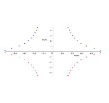
(a)   m=0, l=1, $\omega$

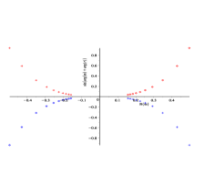
(b)   m=0, l=1, $\sin(\arg(\omega)+\arg(r))$

Fig. 1 : (a) The complex frequencies for $a=0$, for $m=0,l=1$. (b) the boundary condition $\sin(\arg(\omega)+\arg(r))$ for them. The red diamonds are obtained from $R_{1}(r)$ with $\arg(r)=1/2\pi$, the red crosses – from $R_{1}(r)$ with $\arg(r)=3/2\pi$, the blue diamonds – from $R_{2}(r)$ with $\arg(r)=1/2\pi$, the blue crosses – from $R_{2}(r)$ with $\arg(r)=3/2\pi$.

The results for $m=0,l=1$ can be seen on Fig. 1: on a) the complex frequencies, on b) the corresponding boundary conditions at infinity ( $\sin(\arg(\omega)\!+\!\arg(r))\!\lessgtr\!0$). There is a clear symmetry with respect to both the real and the imaginary axes. Also, from the boundary conditions, one can easily differ between the two types of modes – QNM and QBM.

A numerical comparison of QNMs with the frequencies obtained by Berti et al. shows that the average deviation is $|\omega_{n,m}^{B}-\omega_{n,m}|\approx 10^{-10}$.

We checked the dependence of QNM/QBM modes on $|r|$ and, as expected, the modes are stable with respect to an increase in $|r|$, which means that $|r|=110$ is a valid actual infinity. It also confirms that in both cases, $\omega\nsim r$. This requirement comes from the ansatz in the separation of variables from which one obtains the TRE and the TAE.

Another stability test is examining the dependence $\omega(\epsilon)$ (or $\arg(r)$). The so-found QNM and QBM are stable with 20 digits in certain intervals of $\epsilon$, whose width depends on $n$. Such stability intervals are related to the direction of steepest descent, as explained above.

6.2 Rotating KBH

The results for $a=[0..M)$ can be seen on figures $2-7$.

For the QNM modes, when $a\neq 0$, the symmetry with respect to the imaginary axis $\omega_{m,n}^{\pm}=\pm|\Re(\omega_{m,n})|+i\Im(\omega_{m,n})$ breaks down, but it is replaced by the symmetry:

$$\{\Re(\omega_{m,n}^{\pm}),\Im(E_{m,n}^{\pm}),m\}\to\{\!-\!\Re(\omega_{m,n}^{\pm}),\!-\!\Im(E_{m,n}^{\pm}),\!-\!m\},$$

Thus to study the behavior of the modes for $a\in[0,M)$ for all $m$, it is enough to trace both $\omega_{m,n}^{\pm}(a)$ for only $m>0$ (the index $l$ here is omitted to simplify notations).

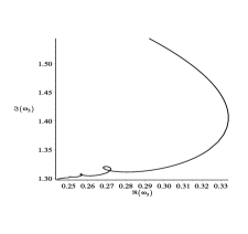
(a) $\omega_{0,3}(a)$

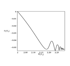
(b) $E_{0,3}(a)$

Fig. 2 : A complex plot of $\omega_{0,3}(a)$ and $E_{0,3}(a)$.

If one considers both the QNM and the QBM, i.e. the roots of the transcendental system in all the 4 quadrants of the complex plane (${I},{II},{III},{IV})$ for $m=0,1$, one observes the symmetry:

$$\Re(\omega_{I})=\Re(\omega_{IV}),\Re(\omega_{II})=\Re(\omega_{III}),$$

$$\Im(\omega_{I})=-\Im(\omega_{II}),\Im(\omega_{III})=-\Im(\omega_{IV})$$

(and analogously for $E$). This symmetry is preserved at least up to $n<4$ within the precision of the numerical method.

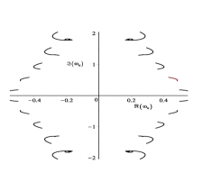
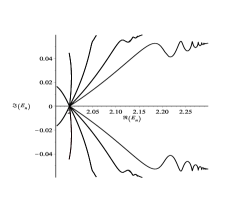
Fig. 3 : Complex plots of $\omega_{0,n}(a)$ and $E_{0,n}(a)$ for $a=[0,M)$ the first 5 modes with both positive and negative real parts

On Fig. 2, one can see an example of the loops characteristic for modes with $m=0,n\geq 3$. On Figs. 3 and 5, one can see all the results plotted together.

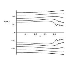
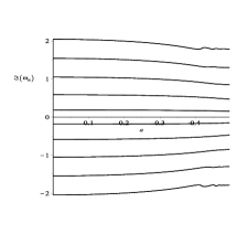
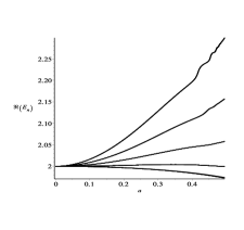
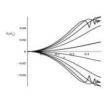
Fig. 4 : On the plots the real and the imaginary parts of $\omega_{0,n}(a)$ and $E_{0,n}(a)$ for $a=[0,M)$ for the modes $n=0..4$.

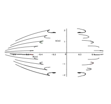
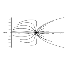
Fig. 5 : A complex plot of all the $\omega_{m,n}(a)$ and $E_{m,n}(a)$ obtained for $a=[0,M)$ for $m=0,1,l=1$ $n=0..4$

As discussed in previous sections, only frequencies for which $\Re(\omega)\!\not\in\!(0,\!-\!m\frac{a}{2Mr_{+}})$ and roots of $R_{2}(r)$ correspond to black hole boundary conditions. From Fig. 6 a), it is clear that the so obtained QNM spectrum obeys this condition. A deviation from this condition was observed in Staicova & Fiziev (2010), where some of the frequencies describing primary jets crossed the line defined by $\!-m\frac{a}{2Mr_{+}}$, thus corresponding to a white hole solution. For the QNM spectrum, however, this is not the case and the spectrum corresponds to perturbation of a black hole. Similarly, for the QBM spectrum in quadrant III, because one is working with the roots of $R_{1}(r)$, for $\omega_{n}<-m\frac{a}{2Mr_{+}}$, the frequencies correspond to a white hole solution, which combined with the boundary condition at infinity, i.e. $\sin(\arg(\omega)+\arg(r))>0$ leads to QBM. Importantly, rotation doesn’t change the type of the spectrum.

Near-extremal regime: From the same figure, one can see in the negative sector of the plot (i.e. frequencies with $\Re(\omega_{n})<0$), that the real parts of the QNMs for increasing $n$ seem to tend to the line $-m\frac{a}{2Mr_{+}}$, confirming the observed in Berti et al. (2003) relation $\Re(\omega)=-m$ for $a\to M$. For the frequencies in the positive sector ($\Re(\omega_{n})>0$), up to $a=0.4997$, the frequencies for $m=1$ do not seem to tend to a single limit.

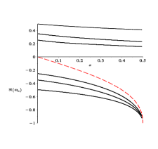
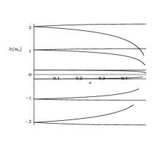
Fig. 6 : On the plots: with black solid lines – $\Re(\omega_{1,n})(a)$ and $\Im(\omega_{1,n})(a)$ for $a=[0,M)$, $n=0..2$ and with red dashed line $-m\frac{a}{2Mr_{+}}$ for $m=1$

Obtaining the modes in the limit $a\approx M$ could be of serious interest, if one is to compare the EM QNMs with the spectra obtained from astrophysical objects but it is also technically challenging. This happens because for $a=M$ the TRE changes its type and near this limit the confluent Heun function becomes numerically unstable since the analytical solutions for $a=M$ are of the biconfluent Heun type. Due to this, the examination of the limit $a\to M$ for modes with high $n$ is very difficult with current numerical realization of that function. For the lowest modes, however, the function is stable enough in the interval $a\in[0.49,0.49999]$ and the results of the numerical experiment for $m=1$ are plotted on Fig. 7. As expected, for $n=0$, for $a>0.91M$ the imaginary part of the frequency quickly tends to zero, thus proving that for extremal objects, the perturbations damp very slowly. The other two modes also seem to tend to zero, although more slowly than $n=0$. In physical units, the difference between the 3 modes for $a=0.4995$ is only 6Hz ($\omega_{0,1}\approx 1.582kHz$), but the damping times of the first mode is approximately 4.86 times bigger than that of the third and is $t^{damp}_{0,1}\approx 4.2ms$ for KBH with mass $M=10M_{\odot}$. Note that the milliseconds time-scales correspond to the usual lifetime of central engines in numerical simulations, once again confirming the relevance of QNMs.

As a test of the numerical stability of our method in the near-extremal case, we compare our numerical results with analytical formulas Eqs. 11 and 12 in Hod (2008) where this regime has been theoretically studied. We considered the cases m=1, l=1, n=0..2 and m=2, l=2, n=0 in the extremal limit $a/M\in[0.995..0.99998]$. It was found that the equations describe well the numerical results, with Eq. 11 fitting better the imaginary parts ($\Im(\omega_{theor})/\Im(\omega_{num})\sim 1\pm 0.05$), while Eq. 12 fits better the real parts ($\Re(\omega_{theor})/\Re(\omega_{num})\sim 1\pm 0.01$). The best value for the parameter ’’$\delta$‘‘ for $m=1,2$ is $\delta=\!-\!1/2$ (for $m=1$ also $\delta\!=\!-\!1/2\!+\!i/10$). The good agreement of Eq. 12 with the numerical data is somewhat unexpected, since in all test cases we have equatorial modes ($m=l$), where Eq. 11 should work better. While this behavior needs to be investigated further, the fact that the analytical formulas approximate the numerical results in the near-extremal regime well serves as an independent confirmation of the viability of the method.

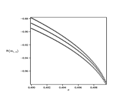
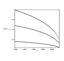
Fig. 7 : On the plot $\Re(\omega_{1,n})(a)$ and $\Im(\omega_{1,n})(a)$ for $a=[0.49,0.4995]$ for the modes $n=0,1,2$, $m=1$

6.3 Algebraically special modes, branch cuts and spurious modes

The algebraically special (AS) modes are obtained from the condition that the Teukolsky-Starobinsky constant vanishes (Chandrasekhar (1983)) and they correspond to the so called total transmission modes (TTM) – modes moving only in one direction: to the right or to the left. In the case of gravitational perturbations ($s=-2$) from non-rotating BH, because the $9^{th}$ QNM coincides approximately with the theoretically expected purely imaginary AS mode, there were speculations that the two modes coincide (see Berti et al. (2003) for a review, and also Maassen van den Brink (2000); Leung et al. (2003)). A study of this mode in the case of gravitational perturbations of KBH showed numerical peculiarities as the ‘‘doublet’’ emerging from the ‘‘AS mode’’ for $m>0$ (Berti et al. (2003)). For the non-rotating gravitational case, Maassen van den Brink Maassen van den Brink (2000); Leung et al. (2003) found that the peculiarities of the $9^{th}$ mode are due to the branch cut in the asymptotics of the Regge-Wheeler potential, which the method of continued fractions is not adapted to handle. This result was confirmed by the use of the $\epsilon$-method in our previous work Fiziev & Staicova (2011a), where the AS character of the $9^{th}$ mode was disproved.

For electromagnetic perturbations, the algebraically special modes have not been discussed much, because in the limit $a\to 0$, the Teukolsky-Starobinsky constant do not vanish for purely imaginary modes (in fact, for $a=0$ the Teukolsky-Starobinsky constant does not depend on $\omega$ at all, see Eq. (60) Chandrasekhar (1983) p.392) and there appear to be no correlation between TTM and QNM modes Onozawa (1996).

Because of the use of the analytical solutions, instead of approximate method such as the continued fraction, we are able to study the behavior of the modes with respect to proximity of a branch cut. As discussed in Section 4, we can use the epsilon-method to rotate the branch cut in the complex $\omega$-plane. This is because thanks to the relation coming from the QNM infinity boundary condition $\arg(r)\!+\!\arg(\omega)\!=\!\frac{3+\epsilon}{2}\!\pi$ (similarly for QBM) we can switch between $\omega$ and $r$. Even more importantly, because of the use of analytical solutions, we have a clear understanding how to differentiate between physical modes such as QNM and QBM and the so-called spurious modes.

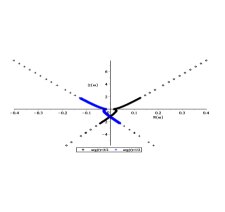
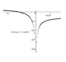
Fig. 8 : a) The spurious modes found as roots of the system. b) the boundary condition for them. Clearly, those modes fulfill both the QNM and the QBM condition for certain $n$.

An example of such a spurious additional spectrum can be seen on Fig. 8. In this case, the modes seem to fulfill the QNM boundary condition for certain $n$ and the QBM boundary condition for other $n$. This makes understanding the nature of those modes difficult. An additional test of their numerical stability with respect to changes in $|r|$ shows that those modes are unstable and they basically decrease with the increase of the actual infinity. Because $\omega\nsim r$ is underlying assumption of the problem, we discard those modes as unphysical. Such spurious modes have been reported in Berti et al. (2003) without further explanation of their nature. In our case, those are modes which are solutions of the spectral system, but which contradict the derivation of the TRE and TAE.

Additional spurious modes can be observed outside of the stability intervals on $\epsilon$ for the QNMs/QBMs. For example, for $n=0,m=0,a=0$, one has a stable mode with precision of 20 digits in the interval $\epsilon=-0.5..0.35$. For $\epsilon>0.35$ the mode starts increasing its real part until it reaches a value for which the boundary condition at infinity is no longer satisfied. We consider those modes to be a product of numerical instability due to inadequate choice of the direction of the steepest descent. Another possible reason for such dramatic changes in the numerical stability of the mode with respect to $\epsilon$ are that the branch cut in the radial function is moved by the parameter $\epsilon$, i.e. they are due to the complex character of the used analytical functions (the confluent Heun functions) in the vicinity of the irregular singular point $r=\infty$ in the complex $r$-plane. Understanding better the theory of the confluent Heun function is critical for the complete understanding of the numerical results.

7 Discussions and conclusion

From the recent developments in the field of gravitational waves detection, it is clear that finding the EM counterpart to those events can prove to be very useful. In this case, it is needed a better understanding of the fundamental physics of quasinormal ringing. In this paper, we offered a new approach to finding the QNMs for the KBH, based on directly solving the system obtained by the analytical solutions of the TRE and TAE in terms of the confluent Heun function. This approach has the advantage of being more traditional (i.e. imposing directly the corresponding boundary conditions on the exact analytical solutions of the problem) and hence it should allow better understanding of the peculiar properties of the EM QNMs and the physics they imply.

It was shown that using this approach one can reproduce the frequencies already obtained by other authors, but without relying on approximate methods. Particularly important is the ability to impose the boundary condition directly on the solutions of the differential equations. We require the standard regularity condition on the TAE and explore in detail the radial boundary condition (the BHBC). We then can solve the system for each of the radial equations, solution of the Teukolsky Master Equation and find both quasinormal and quasibound modes, and additional spurious spectra. By tracking the boundary condition at infinity we are able to work with all those modes at the same time and to obtain their spectra with and without rotation. Such a result shows the advantage of our novel method over more traditional methods. It also raises the question of the theory of the Heun functions as a critical part of understanding the numerical results.

The key results of the article are as follow:

1. High-precision reproduction of known QNM results and study of the numerical stability of the modes in the radial complex plane.

2. New QBM spectrum, obtained for the inverse boundary conditions, its numerical stability also studied.

3. An additional spurious spectrum found to contradict assumptions of the problem and thus classified as numerical artifact.

From our result, the numerical stability of the modes in the r-plane turned out to be a powerful tool for understanding the results. Although obvious in our formulation of the problem, such a study is impossible to perform with the method of continued fraction (at least not directly) because of the missing r-variable. Its usefulness, however, is clear, when one considers the fact that the spurious modes evolve with rotation and can be seen even in the naked singularity regime, where the QNMs and QBMs disappear.

With respect to the QBM spectrum, there is a need of clarification. The Boyer-Lindquist coordinates for the Kerr metric have the following ranges $0\leq r\leq\infty,0\leq\theta\leq\pi,0\leq\phi\leq 2\pi,-\infty<t<\infty$. The stability of the object with respect to perturbations depend on the standard substitution $\Psi=e^{i(\omega t+m\phi)}S(\theta)R(r)$. Clearly, the stability condition $\Im(\omega)>0$ will mean the perturbation will damp with time only as long as $t>0$. Since the range of the t-variable includes also negative values of the time, in those cases, we will have exponentially growing perturbations for the same condition. For the QBM spectra, however, since $\Im(\omega)<0$ the perturbations will damp with time for $t<0$. Also, because of the symmetries of the Kerr metric, it is known that the metric is invariant under the changes $t\to-t,\phi\to-\phi$, meaning that the inversion of time can be considered as inversion of the direction of rotation. Therefore, one can say that the new modes are not unphysical if considered in the correct range for the time-variable. A question of interpretation is whether we will consider the boundary conditions as unstable quasibound (i.e. inverse to QNM) modes for $t>0$ or as stable QNMs for $t<0$.

As a conclusion, the new approach proved that using the analytical solutions of the TRE and TAE, along with the direct imposing of boundary conditions, allowed for better understanding of the problem and for obtaining with high precision both the well-known spectrum and its symmetric but essentially new spectrum.

8 Acknowledgments

The authors would like to thank Prof. E. Berti for discussion of the numerical values of the EM QNM frequencies obtained within the Leaver method, which was important for the comparison of our method with this already well-established one.

The authors would like to thank Dr. Edgardo Cheb-Terrab for useful discussions of the algorithms evaluating the Heun functions in maple and for continuing the improvement of those algorithms.

The authors would like to thank the anonymous reviewer who drew our attention also to the work of Shahar Hod, based on analytical calculations. The comparison of our numerical results with that work increased our confidence in the validity of the results.

This article was supported by the Foundation "Theoretical and Computational Physics and Astrophysics", by the Bulgarian National Scientific Fund under contracts DO-1-872, DO-1-895, DO-02-136, and Sofia University Scientific Fund, contract 185/26.04.2010, Grants of the Bulgarian Nuclear Regulatory Agency for 2013, 2014 and 2015.

9 Author Contributions

P.F. posed the problem of evaluation of the EM QNMs of rotating BHs as a continuation of previous studies of the applications of the confluent Heun functions in astrophysics. He proposed the epsilon method and supervised the project.

D.S. is responsible for the numerical results, their analysis and the plots presented here.

Both authors discussed the results at all stages. The manuscript was prepared by D.S. and edited by P.F..

References

- Abadie et al. (2011) Abadie J. et al. (The LIGO Scientific Collaboration,), Search for Gravitational Wave Bursts from Six Magnetars Astrophys.J.734:(L35,2011), arXiv:1011.4079v2 [astro-ph.HE]
- Abadie et al. (2012) Abadie J. et al. (For LIGO scientific collaboration, the Virgo Collaboration), Search for gravitational waves associated with gamma-ray bursts during LIGO science run 6 and Virgo science runs 2 and 3, Astrophys. J. 760 12 (2012), arXiv:1205.2216 [astro-ph.HE]
- Abadie et al. (2013) Abadie J. et al. (For LIGO scientific collaboration, the Virgo Collaboration), Search for long-lived gravitational-wave transients coincident with long gamma-ray bursts, Phys. Rev. D. 88, 122004 (2013), arXiv:1309.6160 [astro-ph.HE]
- Abadie et al. (2014) Abadie J. et al. (For LIGO scientific collaboration, the Virgo Collaboration), Search for gravitational waves associated with gamma-ray bursts detected by the InterPlanetary Network, Phys. Rev. Lett. 113, 011102 (2014), arXiv:1403.6639 [astro-ph.HE]
- Andersson (1992) Andersson N., A numerically accurate investigation of black-hole normal modes, Proc. Roy. Soc. London A439 no.1905: 47-58 (1992)
- Bardeen et al. (1972) Bardeen, J.M., Press, W. H., Teukolsky, S. A., Rotating Black Holes: Locally Nonrotating Frames, Energy Extraction, and Scalar Synchrotron Radiation, Astrophys. J. 178: 347-370 (1972)
- Berti (2004) Berti E., Black hole quasinormal modes: hints of quantum gravity?, Proc. of the Workshop on ’Dynamics and Thermodynamics of Black Holes and Naked Singularities’ (Milan, May 2004), arXiv:gr-qc/0411025v1 (2004)
- Berti et al. (2003) Berti E.,Cardoso V., Kokkotas K. D., Onozawa H., Highly damped quasinormal modes of Kerr black holes Phys.Rev.D 68 124018, (2003), arXiv:hep-th/0307013v2
- Berti et al. (2006) Berti E., Cardoso V., Will C. M., On gravitational-wave spectroscopy of massive black holes with the space interferometer LISA, Phys.Rev.D 73:064030, (2006), arXiv:0512160v2 [gr-qc]
- Berti et al. (2009) Berti E., Cardoso V. and Starinets A . O., Quasinormal modes of black holes and black branes, Class. Quantum Grav. 26 163001 (108pp) (2009)
- Bogdanovic et al. (2011) Bogdanovic T. , Bode T., Haas R., Laguna P., Shoemaker D., Properties of Accretion Flows Around Coalescing Supermassive Black Holes, Class. and Quantum Gravity, 28:094020 (2011), arXiv:1010.2496v2 [astro-ph.CO]
- Chandrasekhar (1975) Chandrasekhar S., On the Equations Governing the Perturbations of the Schwarzschild Black Hole, Proc. Roy. Soc. London A343: 289-298 (1975)
- Chandrasekhar (1976a) Chandrasekhar S., On a transformation of Teukolsky’s equation and the electromagnetic perturbations of Kerr black hole, Proc. R. Soc. Lond. A 348, 39-55 (1976a)
- Chandrasekhar (1976b) Chandrasekhar S., On the equations governing the perturbations of Reissner - Nordströ m black hole, Proc. R. Soc. London A 3365, 453-465 (1976b)
- Chandrasekhar (1983) Chandrasekhar S., The mathematical theory of black holes, Clarendon Press/Oxford University Press (International Series of Monographs on Physics. Volume 69), (1983)
- Chandrasekhar & Detweiler (1975) Chandrasekhar S., and Detweiler S. L., The quasinormal modes of the Schwarzschild black hole, Proc. Roy. Soc. London A344: 441-452 (1975)
- Chirenti & Rezzolla (2007) Chirenti C. B. M. H., Rezzolla L., How to tell gravastar from black hole, Class. Quant. Grav. 24:, 4191-4206, (2007), arXiv:0706.1513v2 [gr-qc]
- Chirenti & Rezzolla (2008) Chirenti C. B. M. H., Rezzolla L., Ergoregion instability in rotating gravastars, Phys.Rev.D 78:084011, (2008), arXiv:0808.4080v1 [gr-qc]
- Christensen (2011) Christensen N.L., (For the LIGO Scientific Collaboration, the Virgo Collaboration), Multimessenger Astronomy, Proc. for the 46th Rencontres de Moriond and GPhyS Colloquium on Gravitational Waves and Experimental Gravity, arXiv:1105.5843v1 [gr-qc]
- Coward et al. (2011) Coward D. M., Gendre B., Sutton P.J. , Howell E.J. , Regimbau T., Laas-Bourez M., Klotz A., Boer M., Branchesi M., Toward an optimal search strategy of optical and gravitational wave emissions from binary neutron star coalescence, MNRAS, 415:L26, arXiv:1104.5552v1 [astro-ph.HE]
- Decarreau et al. (1978a) Decarreau A., Dumont-Lepage M. Cl., Maroni P., Robert A. and Ronveaux A., Ann. Soc. Bruxelles 92 53, (1978a)
- Decarreau et al. (1978b) Decarreau A., Maroni P. and Robert A., Ann. Soc. Bruxelles 92 151 (1978b )
- Detweiler (1976) Detweiler S., On the equations governing the electromagnetic perturbations of the Kerr black hole, Proc. R. Soc. London A 349, 217-230 (1976)
- Detweiler (1980) Detweiler S., Black holes and gravitational waves. III - The resonant frequencies of rotating holes, Astrophys. J.:239, 292-295, (1980)
- Ferrari & Gualtieri (2007) Ferrari V., Gualtieri L., Quasi-normal modes and gravitational wave astronomy, Gen.Rel.Grav.40: 945-970 (2008), arXiv:0709.0657v2 [gr-qc]
- Fiziev (2006) Fiziev P. P., Exact Solutions of Regge-Wheeler Equation and Quasi-Normal Modes of Compact Objects, Class. Quant. Grav. 23 2447-2468 (2006), arXiv:0509123 [gr-qc]
- Fiziev (2009) Fiziev P. P., Teukolsky-Starobinsky identities: A novel derivation and generalizations, Phys. Rev. D80, 124001 (2009), arXiv:0906.5108 [gr-qc]
- Fiziev (2010a) Fiziev P. P., Classes of exact solutions to the Teukolsky master equation Class. Quantum Grav. 27 135001 (2010a), arXiv:0908.4234v4 [gr-qc]
- Fiziev (2010b) Fiziev P. P., Novel relations and new properties of confluent Heun’s functions and their derivatives of arbitrary order, J. Phys. A: Math. Theor. 43 (2010b) 035203, arXiv:0904.0245 [math-ph]
- Fiziev & Staicova (2011a) Fiziev P., Staicova D., Application of the confluent Heun functions for finding the QNMs of non-rotating black hole, Phys. Rev. D 84, 127502 (2011a) , arXiv:1109.1532 [gr-qc]
- Fiziev & Staicova (2011b) Fiziev P., Staicova D., Two-dimensional generalization of the Muller root-finding algorithm and its applications (2011b), arXiv:1005.5375v2 [cs.NA]
- Fiziev & Staicova (2012) Fiziev P., Staicova D., Solving systems of transcendental equations involving the Heun functions., Am. J. Comput. Math. 02 : 02, pp.95 (2012), arXiv:1201.0017 [cs.NA]
- Gao et al. (2011) Gao, H., Zhang B. .B and Zhang B., Evidence Of Superposed Variability Components In GRB Prompt Emission Lightcurves, The Astrophys. J., 02: 748(2, (2011), arXiv:1103.0074v2 [astro-ph.HE], (2011)
- Heun (1889) Heun K., Math. Ann. 33 161, (1889)
- Hod (2008) Hod S., Slow relaxation of rapidly rotating black holes, Phys.Rev. D 78:084035,(2008), arXiv:0811.3806 [gr-qc]
- Hod (2011) Hod S., Quasinormal resonances of a massive scalar field in a near-extremal Kerr black hole spacetime Phys. Rev. D 84, 044046 (2011), arXiv:1109.4080v1 [gr-qc]
- Hod & Hod (2010) Hod S., Hod O., Analytic treatment of the black-hole bomb, Phys. Rev. D 81, 061502 (2010) Rapid communication, arXiv:0910.0734v1 [gr-qc]
- Jaramillo et al. (2012) Jaramillo J. L., Macedo R. P., Moesta P., Rezzolla L., Black-hole horizons as probes of black-hole dynamics I: post-merger recoil in head-on collisions, Phys. Rev. D 85, 084030 (2012), arXiv:1108.0060v1 [gr-qc]
- Konoplya & Zhidenko (2011) Konoplya, R. A., Zhidenko, A., Quasinormal modes of black holes: from astrophysics to string theory, Reviews of Modern Physics, 83: 793 - 836, issue 3, (2011), arXiv:1102.4014v1 [gr-qc]
- Leaver (1985) Leaver E. W., An analytic representation for the quasinormal modes of Kerr black holes, Proc. Roy. Soc. London A402: 285-298 (1985)
- Leaver (1986) Leaver E. W., Solutions to a generalized spheroidal wave equation: Teukolsky’s equations in general relativity, and the two-center problem in molecular quantum mechanics, J.Math. Phys.27 (5):1238 (1986)
- Lei & Zhang (2011) Lei W.-H., Zhang B., Black hole Spin in Sw J1644+57 and Sw J2058+05 , ApJ L27: 740, arXiv:1108.3115v2 [astro-ph.HE],(2011)
- Leung et al. (2003) Leung P. T., Maassen van den Brink A., Mak K. W., Young K., Unconventional Gravitational Excitation of a Schwarzschild Black Hole, Class.Quant.Grav. 20 L217 (2003), arXiv:gr-qc/0301018v4
- Lyutikov & McKinney (2011) Lyutikov M., McKinney J. C., Slowly balding black holes, Phys. Rev. D, 84:084019, arXiv:1109.0584v1 [astro-ph.HE], (2011)
- Maassen van den Brink (2000) Maassen van den Brink A, Analytic treatment of black-hole gravitational waves at the algebraically special frequency, Phys. Rev. D 62 064009 (2000), arXiv:gr-qc/0001032v1
- Moesta et al. (2011) Moesta P., Alic D., Rezzolla L., Zanotti O., Palenz C., On the detectability of dual jets from binary black holes , ApJ, 749, L32, 2012, arXiv:1109.1177v1 [gr-qc]
- Onozawa (1996) Onozawa H., A detailed study of quasinormal frequencies of the Kerr black hole, Phys.Rev. D 55: 3593-3602 (1997), arXiv:gr-qc/9610048v1
- Pani et al. (2009) Pani P., Berti E., Cardoso V., Chen Y., Norte R., Gravitational wave signatures of the absence of an event horizon: Nonradial oscillations of a thin-shell gravastar , Phys.Rev.D 80:124047,(2009) , arXiv:0909.0287v2 [gr-qc]
- Press & Teukolsky (1973) Press W. H., Teukolsly S. A., Perturbations of a Rotating Black Hole. II. Dynamical Stability of the Kerr Metric,Astrophys. J. 185:649-674 (1973)
- Regge & Wheeler (1957) Regge, T., Wheeler J. A., Stability of a Schwarzschild Singularity, Phys.Rev 108:I.4: 1063-1069 (1957) 737-738 (1970)
- Rezzolla & Kumar (2014) Rezzolla L., Kumar P., A novel paradigm for short gamma-ray bursts with extended X-ray emission, Astrophys. J., 802, 95 (2015), arXiv:1410.8560 [astro-ph.HE]
- Rosa & Dolan (2012) Rosa J. G. and Dolan S. R., Massive vector fields on the Schwarzschild spacetime: Quasinormal modes and bound states, Phys. Rev. D 85, 044043 (2012)
- Ronveaux (1995) ed. Ronveaux A, Heun’s Differential Equations ed. Ronveaux A., Oxford: Oxford Univ. Press, (1995)
- Schnittman (2011) Schnittman, J. D., Electromagnetic counterparts to black hole mergers Class. Quantum Gravity, 28, Issue 9, pp. 094021 (2011), arXiv:1010.3250v1 [astro-ph.HE]
- Schutz et al. (2011) Schutz B. F., Centrella J., Cutler C., Hughes S. A., Will Einstein Have the Last Word on Gravity?, In: Astro2010: The Astronomy and Astrophysics Decadal Survey, arXiv: 0903.0100v1 [gr-qc]
- Slavyanov & Lay (2000) Slavyanov S. Y., Lay W., Special Functions, A Unified Theory Based on Singularities (Oxford: Oxford Mathematical Monographs) (2000)
- Staicova & Fiziev (2010) Staicova D., Fiziev P., The Spectrum of Electromagnetic Jets from Kerr Black Holes and Naked Singularities in the Teukolsky Perturbation Theory,Astrophys. Space Sci., 332, pp.385-401, arXiv:1002.0480 [astro-ph.HE], (2010)
- Staicova & Fiziev (2011) Staicova D., Fiziev P., New results for electromagnetic quasinormal modes of black holes, arXiv:1112.0310 [astro-ph.HE], (2011)
- Teukolsky (1972) Teukolsky, S. A., Rotating Black Holes: Separable Wave Equations for Gravitational and Electromagnetic Perturbations, Phys.Rev.Lett. 29: 1114-1118 (1972)
- Teukolsky (1973) Teukolsky, S. A., Perturbations of a rotating black hole I Fundamental Equations for Gravitational, Electromagnetic and Neutrino-field Perturbations, Astrophys. J. 185: 635-648 (1973)
- Teukolsky (2014) Teukolsky S. A REVIEW ARTICLE, The Kerr Metric, to appear in Classical and Quantum Gravity for its "Milestones of General Relativity" focus issue to be published during the Centenary Year of GR, (2014) arXiv:1410.2130
- Teukolsky & Press (1974) Teukolsky S. A., Press W. H., Perturbations of a rotating black hole. III - Interaction of the hole with gravitational and electromagnetic radiation, Astrophys. J. 193: 443 (1974)
- LIGO & VIRGO (2010a) the LIGO Scientific Collaboration, the Virgo Collaboration, Search for Gravitational Waves from Compact Binary Coalescence in LIGO and Virgo Data from S5 and VSR1, Phys.Rev.D82 : 102001, (2010a),
- LIGO & VIRGO (2010b) the LIGO Scientific Collaboration, the Virgo Collaboration, Search for gravitational-wave bursts associated with gamma-ray bursts using data from LIGO Science Run 5 and Virgo Science Run 1, Astrophysical Journal 715 (2010b) 1438-1452 arXiv:0908.3824v2 [astro-ph.HE]
- LIGO & VIRGO (2011) The LIGO Scientific Collaboration, the Virgo Collaboration , Search for gravitational waves from binary black hole inspiral, merger and ringdown Phys.Rev.D 83:122005,(2011)
- LIGO & VIRGO (2012) the LIGO Scientific Collaboration, the Virgo Collaboration, Implementation and testing of the first prompt search for electromagnetic counterparts to gravitational wave transients, A&A Vol. 539, A124, March 2012 , arXiv:1109.3498v1 [astro-ph.IM], (2012)
- Vishveshwara (1970) Vishveshwara, C. V., Stability of the Schwarzschild Metric, Phys.Rev. D 1:I.10: 2870-2879 (1970)
- Zerilli (1970) Zerilli, F. J., Effective Potential for Even-Parity Regge-Wheeler Gravitational Perturbation Equations, Phys.Rev. Lett. 24:I.13:
- Zhang (2011) Zhang B., Open Questions in GRB Physics Comptes Rendus Physique, 12, 206-225 (2011), arXiv:1104.0932v1 [astro-ph.HE]