Critical points of random polynomials and characteristic polynomials of random matrices

Abstract.

Let $p_{n}$ be the characteristic polynomial of an $n\times n$ random matrix drawn from one of the compact classical matrix groups. We show that the critical points of $p_{n}$ converge to the uniform distribution on the unit circle as $n$ tends to infinity. More generally, we show the same limit for a class of random polynomials whose roots lie on the unit circle. Our results extend the work of Pemantle–Rivin [30] and Kabluchko [19] to the setting where the roots are neither independent nor identically distributed.

1. Introduction

A critical point of a polynomial $f$ is a root of its derivative $f^{\prime}$. There are many results concerning the location of critical points of polynomials whose roots are known. For example, the famous Gauss–Lucas theorem offers a geometric connection between the roots of a polynomial and the roots of its derivative.

Theorem 1 (Gauss–Lucas; Theorem 6.1 from [24]).

If $f$ is a non-constant polynomial with complex coefficients, then all zeros of $f^{\prime}$ belong to the convex hull of the set of zeros of $f$.

There are also a number of refinements of Theorem 1. We refer the reader to [1, 3, 5, 8, 10, 14, 18, 22, 23, 25, 29, 32, 34, 35, 39, 42] and references therein.

Pemantle and Rivin [30] initiated the study of a probabilistic version of the Gauss–Lucas theorem. In order to introduce their results, we fix the following notation. For a polynomial $f$ of degree $n$, we define the empirical measure constructed from the roots of $f$ as

$$\mu_{f}:=\frac{1}{n}\sum_{z\in\mathbb{C}:f(z)=0}\mathcal{N}_{f}(z)\delta_{z},$$

where $\mathcal{N}_{f}(z)$ is the multiplicity of the zero at $z$ and $\delta_{z}$ is the unit point mass at $z$.

For an integer $k\geq 1$, we use the convention that

$$\mu_{f}^{(k)}:=\mu_{f^{(k)}}.$$

That is, $\mu_{f}^{(k)}$ is the empirical measure constructed from the roots of the $k$-th derivative of $f$. Similarly, we write $\mu_{f}^{\prime}$ to denote the empirical measure constructed from the critical points of $f$.

Let $X_{1},X_{2},\ldots$ be independent and identically distributed (iid) random variables taking values in $\mathbb{C}$. Let $\mu$ be the probability distribution of $X_{1}$. For each $n\geq 1$, consider the polynomial

$$p_{n}(z):=(z-X_{1})\cdots(z-X_{n}).$$ (1)

Pemantle and Rivin [30] show, assuming $\mu$ has finite one-dimensional energy, that $\mu^{\prime}_{p_{n}}$ converges weakly to $\mu$ as $n$ tends to infinity.

Let us recall what it means for a sequence of random probability measures to converge weakly.

Definition 2 (Weak convergence of random probability measures).

Let $T$ be a topological space (such as $\mathbb{R}$ or $\mathbb{C}$), and let $\mathcal{B}$ be its Borel $\sigma$-field. Let $(\mu_{n})_{n\geq 1}$ be a sequence of random probability measures on $(T,\mathcal{B})$, and let $\mu$ be a probability measure on $(T,\mathcal{B})$. We say $\mu_{n}$ converges weakly to $\mu$ in probability as $n\to\infty$ (and write $\mu_{n}\to\mu$ in probability) if for all bounded continuous $f:T\to\mathbb{R}$ and any $\varepsilon>0$,

$$\lim_{n\to\infty}\mathbb{P}\left(\left|\int fd\mu_{n}-\int fd\mu\right|>\varepsilon\right)=0.$$

In other words, $\mu_{n}\to\mu$ in probability as $n\to\infty$ if and only if $\int fd\mu_{n}\to\int fd\mu$ in probability for all bounded continuous $f:T\to\mathbb{R}$. Similarly, we say $\mu_{n}$ converges weakly to $\mu$ almost surely as $n\to\infty$ (and write $\mu_{n}\to\mu$ almost surely) if for all bounded continuous $f:T\to\mathbb{R}$,

$$\lim_{n\to\infty}\int fd\mu_{n}=\int fd\mu$$

almost surely.

Kabluchko [19] generalized the results of Pemantle and Rivin to the following.

Theorem 3 (Kabluchko).

Let $\mu$ be any probability measure on $\mathbb{C}$. Let $X_{1},X_{2},\ldots$ be a sequence of iid random variables with distribution $\mu$. For each $n\geq 1$, let $p_{n}$ be the degree $n$ polynomial given in (1). Then $\mu^{\prime}_{p_{n}}$ converges weakly to $\mu$ in probability as $n\to\infty$.

The following corollary of Theorem 3 will be relevant to this note.

Corollary 4.

Let $\theta_{1},\theta_{2},\ldots$ be a sequence of iid random variables distributed uniformly on $[0,2\pi)$. For each $n\geq 1$, let

$$p_{n}(z):=\prod_{j=1}^{n}(z-e^{i\theta_{j}}).$$

Then $\mu^{\prime}_{p_{n}}$ converges in probability to the uniform probability distribution on the unit circle centered at the origin in the complex plane as $n\to\infty$.

Corollary 4 also follows from the work of Subramanian in [40].

2. Main Results

The goal of this note is to prove a version of Theorem 3 when the random variables $X_{1},X_{2},\ldots$ are neither independent nor identically distributed. Of particular interest will be the case when the roots of $p_{n}$ are eigenvalues of a random matrix.

The eigenvalues of a square matrix $M$ are the zeros of its characteristic polynomial $p_{M}(z):=\det(zI-M)$, where $I$ denotes the identity matrix. We let $\mu_{M}$ denote the empirical spectral measure of $M$. That is, $\mu_{M}$ is the empirical measure constructed from the roots of the characteristic polynomial $p_{M}$. Similarly, we let $\mu_{M}^{\prime}$ be the empirical measure constructed from the roots of $p^{\prime}_{M}$.

As a motivating example, we begin with the case when $M$ is Hermitian.

2.1. Characteristic polynomials of Hermitian random matrices

If the matrix $M$ is Hermitian (that is, $M=M^{\ast}$, where $M^{\ast}$ denotes the conjugate transpose of $M$), then the eigenvalues of $M$ are real and $\mu_{M}$ is a probability measure on the real line. In this case, Theorem 6 below describes the well-known connection between $\mu_{M}$ and $\mu_{M}^{\prime}$. Before stating the result, we first recall the following definition.

Definition 5 (Lévy distance).

Let $\mu$ and $\nu$ be two probability measures on the real line with cumulative distribution functions $F$ and $G$ respectively. Then the Lévy distance $L(\mu,\nu)$ between $\mu$ and $\nu$ is given by

$$L(\mu,\nu):=\inf\{\varepsilon\geq 0:G(x-\varepsilon)-\varepsilon\leq F(x)\leq G(x+\varepsilon)+\varepsilon\text{ for all }x\in\mathbb{R}\}.$$

It is well-known, for measures on the real line, that convergence in Lévy distance is equivalent to convergence in distribution; we refer the reader to [21, Chapter 13.2] and [21, Exercise 13.2.6] for further details.

Theorem 6.

For each $n\geq 1$, let $X_{n}$ be a $n\times n$ random Hermitian matrix. Then $\mu_{X_{n}}^{\prime}$ is a random probability measure on the real line and

$$L(\mu_{X_{n}},\mu_{X_{n}}^{\prime})\longrightarrow 0$$

almost surely as $n\to\infty$

Proof.

Since the eigenvalues of $X_{n}$ are real, the Gauss–Lucas theorem (Theorem 1) guarantees that $\mu^{\prime}_{X_{n}}$ is a probability measure on the real line.

Let $I\subset\mathbb{R}$ be an interval. Let $N_{I}$ denote the number of zeros of $p_{X_{n}}$ in $I$ (i.e. the number of eigenvalues of $X_{n}$ in $I$), and let $N_{I}^{\prime}$ denote the number of critical points of $p_{X_{n}}$ in $I$. Since the zeros of $p^{\prime}_{X_{n}}$ interlace the zeros of $p_{X_{n}}$, we have

$$\left|N_{I}-N_{I}^{\prime}\right|\leq 1,$$

and the claim follows from [2, Lemma B.18]. ∎

As a concrete example, we present the following corollary for Wigner random matrices.

Corollary 7.

Let $\xi$ be a complex-valued random variable with unit variance, and let $\zeta$ be a real-valued random variable. For each $n\geq 1$, let $X_{n}$ be a $n\times n$ Hermitian matrix whose diagonal entries are iid copies of $\zeta$, those above the diagonal are iid copies of $\xi$, and all the entries on and above the diagonal are independent. Then $\mu_{\frac{1}{\sqrt{n}}X_{n}}^{\prime}$ is a probability measure on the real line and

$$\mu_{\frac{1}{\sqrt{n}}X_{n}}^{\prime}\longrightarrow\mu_{\mathrm{sc}}$$

almost surely as $n\to\infty$, where $\mu_{\mathrm{sc}}$ is the measure on the real line with density

$$\rho_{\mathrm{sc}}(x):=\left\{\begin{array}[]{ll}\frac{1}{2\pi}\sqrt{4-x^{2}},&|x|\leq 2\\ 0,&|x|>2.\end{array}\right.$$

Proof.

In view of [2, Theorem 2.5] and [21, Exercise 13.2.6], we have

$$L\left(\mu_{\frac{1}{\sqrt{n}}X_{n}},\mu_{\mathrm{sc}}\right)\longrightarrow 0$$

almost surely as $n\to\infty$. Thus, the claim follows from Theorem 6 by applying the triangle inequality for Lévy distance. ∎

The same arguments can also be used to generalize Theorem 6 and Corollary 7 to higher-order derivatives.

2.2. Random matrices from the compact classical groups

In this note, we extend Theorem 6 to random matrices which are not Hermitian. In particular, we consider random matrices distributed according to Haar measure on the compact classical matrix groups. We begin by recalling some definitions.

Definition 8 (Compact classical matrix groups).

1. An $n\times n$ matrix $M$ over $\mathbb{R}$ is orthogonal if

   $$MM^{\mathrm{T}}=M^{\mathrm{T}}M=I_{n},$$

   where $I_{n}$ denotes the $n\times n$ identity matrix and $M^{\mathrm{T}}$ is the transpose of $M$. The set of $n\times n$ orthogonal matrices over $\mathbb{R}$ is denoted by $\mathrm{O}(n)$.

2. The set $\mathrm{SO}(n)\subset\mathrm{O}(n)$ of special orthogonal matrices is defined by

   $$\mathrm{SO}(n):=\{M\in\mathrm{O}(n):\det(M)=1\}.$$

3. An $n\times n$ matrix $M$ over $\mathbb{C}$ is unitary if

   $$MM^{\ast}=M^{\ast}M=I_{n},$$

   where $M^{\ast}$ denotes the conjugate transpose of $M$. The set of $n\times n$ unitary matrices over $\mathbb{C}$ is denoted $\mathrm{U}(n)$.

4. If $n$ is even, we say an $n\times n$ matrix $M$ over $\mathbb{C}$ is symplectic if $M\in\mathrm{U}(n)$ and

   $$MJM^{\ast}=M^{\ast}JM=J,$$

   where

   $$J:=\begin{bmatrix}0&I_{n/2}\\ -I_{n/2}&0\end{bmatrix}.$$

   The set of $n\times n$ symplectic matrices over $\mathbb{C}$ is denoted $\mathrm{Sp}(n)$.

Recall that if $M$ is a matrix from one of the compact matrix groups introduced above, then the eigenvalues of $M$ all lie on the unit circle in the complex plane centered at the origin.

For any compact Lie group $G$, there exists a unique translation-invariant probability measure on $G$ called Haar measure; see, for example, [12, Chapter 2.2]. In this note, we will be interested in the case when $G$ is one of classical compact matrix groups defined above.

For the compact matrix groups, there are a number of intuitive ways to describe a matrix distributed according to Haar measure. Recall that a complex standard normal random variable $Z$ can be represented as $Z=X+iY$, where $X$ and $Y$ are independent real normal random variables with mean zero and variance $1/2$. Form an $n\times n$ random matrix with independent complex standard normal entries and perform the Gram–Schmidt algorithm on the columns. The result is a random unitary matrix distributed according to Haar measure on $\mathrm{U}(n)$. Indeed, invariance follows from the invariance of complex Gaussian random vectors under $\mathrm{U}(n)$. Similar Gaussian constructions yield random matrices distributed according to Haar measure on the other compact matrix groups.

We now present our main result for the classical compact matrix groups.

Theorem 9.

For each $n\geq 1$, let $M_{n}$ be an $n\times n$ matrix Haar distributed on $\mathrm{O}(n)$, $\mathrm{SO}(n)$, $\mathrm{U}(n)$, or $\mathrm{Sp}(n)$. Then $\mu_{M_{n}}^{\prime}$ converges in probability as $n\to\infty$ to the uniform probability distribution on the unit circle centered at the origin.

Remark 10.

If $M_{n}$ is an $n\times n$ random matrix Haar distributed on $\mathrm{O}(n)$, $\mathrm{SO}(n)$, $\mathrm{U}(n)$, or $\mathrm{Sp}(n)$, then $\mu_{M_{n}}$ also converges in probability to the uniform distribution on the unit circle centered at the origin. Moreover, in [27], the authors prove that the convergence holds in the almost sure sense and give a rate of convergence.

Figure 1 depicts a numerical simulation of the zeros and critical points of the characteristic polynomial of a random orthogonal matrix chosen according to Haar measure.

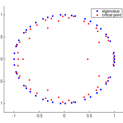
Figure 1. The zeros and critical points of the characteristic polynomial of a random orthogonal matrix of size $50\times 50$.

2.3. Random polynomials with roots on the unit circle

More generally, we consider random polynomials of the form

$$p_{n}(z):=\prod_{j=1}^{n}(z-X_{j}),$$

where $X_{1},X_{2},\ldots$ are random variables on the unit circle, not necessarily independent or identically distributed. Indeed, we will deduce Theorem 9 from the following more general result.

Theorem 11.

For each $n\geq 1$, let $\theta_{1}^{(n)},\ldots,\theta_{n}^{(n)}$ be random variables on $[0,2\pi)$. Set

$$p_{n}(z):=\prod_{j=1}^{n}(z-e^{i\theta_{j}^{(n)}}).$$

Assume

1. we have

   $$\lim_{\delta\searrow 0}\limsup_{n\to\infty}\mathbb{P}\left(\left|\sum_{j=1}^{n}e^{-i\theta_{j}^{(n)}}\right|\leq\delta\right)=0,$$

2. for almost every $z\in\mathbb{D}:=\{w\in\mathbb{C}:|w|<1\}$,

   $$\lim_{\delta\searrow 0}\limsup_{n\to\infty}\mathbb{P}\left(\left|\sum_{m=0}^{\lfloor\log^{2}n\rfloor}z^{m}\sum_{j=1}^{n}e^{-i\theta_{j}^{(n)}(m+1)}\right|\leq\delta\right)=0,$$

3. for all integers $m\geq 1$,

   $$\frac{1}{n}\sum_{j=1}^{n}e^{i\theta_{j}^{(n)}m}\longrightarrow 0$$

   in probability as $n\to\infty$.

Then $\mu_{p_{n}}^{\prime}$ converges in probability as $n\to\infty$ to the uniform probability distribution on the unit circle centered at the origin.

We pause for a moment to discuss the three assumptions of Theorem 11. Roughly speaking, condition (iii) is the most important, while conditions (i) and (ii) are technical anti-concentration estimates. Indeed, condition (iii) implies that the empirical measure constructed from $e^{i\theta_{1}^{(n)}},\ldots,e^{i\theta_{n}^{(n)}}$ converges in probability as $n\to\infty$ to the uniform distribution on the unit circle centered at the origin. We also note that the sequence $\log^{2}n$ appearing in condition (ii) is not vital; it can be replaced with $(\log n)^{1+\varepsilon}$ for any $\varepsilon>0$.

We will also verify the following alternative formulation of Theorem 11.

Theorem 12 (Alternative formulation).

For each $n\geq 1$, let $\theta_{1}^{(n)},\ldots,\theta_{n}^{(n)}$ be random variables on $[0,2\pi)$. Set

$$p_{n}(z):=\prod_{j=1}^{n}(z-e^{i\theta_{j}^{(n)}}).$$

Assume

1. we have

   $$\lim_{\delta\searrow 0}\limsup_{n\to\infty}\mathbb{P}\left(\left|\sum_{j=1}^{n}e^{-i\theta_{j}^{(n)}}\right|\leq\delta\right)=0,$$

2. for almost every $z\in\mathbb{D}:=\{w\in\mathbb{C}:|w|<1\}$,

   $$\frac{1}{n}\log\left|\sum_{j=1}^{n}\frac{1}{z-e^{i\theta_{j}^{(n)}}}\right|\longrightarrow 0$$

   in probability as $n\to\infty$,

3. for all integers $m\geq 1$,

   $$\frac{1}{n}\sum_{j=1}^{n}e^{i\theta_{j}^{(n)}m}\longrightarrow 0$$

   in probability as $n\to\infty$.

Then $\mu_{p_{n}}^{\prime}$ converges in probability as $n\to\infty$ to the uniform probability distribution on the unit circle centered at the origin.

We will use Theorem 11 to prove Theorem 9. However, Theorem 12 is also useful. For example, we can recover Corollary 4 from Theorem 12. Indeed, if $\theta_{1}^{(n)},\ldots,\theta_{n}^{(n)}$ are iid random variables uniformly distributed on $[0,2\pi)$, then the assumptions of Theorem 12 can be verified using [31, Theorem 2.22], [19, Lemma 2.1], and the law of large numbers. Theorem 12 is also useful when the random variables $\theta_{1}^{(n)},\ldots,\theta_{n}^{(n)}$ are dependent. To illustrate this point, we will use Theorem 12 to verify the following corollary.

Corollary 13.

Let $\theta_{1},\theta_{2},\ldots$ be a sequence of iid random variables distributed uniformly on $[0,2\pi)$. For each $n\geq 1$, set

$$p_{2n}(z):=\prod_{j=1}^{n}(z-e^{i\theta_{j}})(z-e^{-i\theta_{j}}).$$

Then $\mu_{p_{2n}}^{\prime}$ converges in probability as $n\to\infty$ to the uniform probability distribution on the unit circle centered at the origin.

2.4. Discussion and open problems

We conjecture that for many classes of random polynomials the critical points should be stochastically close to the distribution of the roots. Intuitively, this would imply that the distribution of the critical points is nearly identical to the distribution of the roots for a “typical” polynomial of high degree.

As another example, consider the Kac polynomials. In this case, one can show even more by applying the results of Kabluchko and Zaporozhets [20].

Theorem 14 (Kabluchko–Zaporozhets).

Let $\xi_{0},\xi_{1},\ldots$ be a sequence of non-degenerate iid random variables such that $\mathbb{E}\log(1+|\xi_{0}|)<\infty$. For each $n\geq 1$, let $f_{n}(z)=\sum_{j=0}^{n}\xi_{j}z^{j}$. Fix an integer $k\geq 1$. Then $\mu_{f_{n}}$ and $\mu_{f_{n}}^{(k)}$ both converge in probability as $n\to\infty$ to the uniform probability distribution on the unit circle centered at the origin.

Proof.

Both claims follow from [20, Theorem 2.2] by simply estimating the coefficients of $f_{n}^{(k)}$. In fact, a similar argument allows one to consider solutions of the equation $f_{n}^{(k)}=c_{n}$, where $c_{n}$ is a constant; see [20, Remark 2.11] for details. ∎

We conjecture that this universality phenomenon should also hold for the characteristic polynomial of many random matrix ensembles. For instance, Figure 2 depicts a numerical simulation of the zeros and critical points of the characteristic polynomial of a random matrix with iid real standard normal entries.

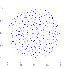
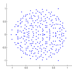
Figure 2. The roots and critical points of the characteristic polynomial of an $n\times n$ random matrix with iid real standard normal entries when $n=300$. The figure on the left depicts the location of the eigenvalues (scaled by $1/\sqrt{n}$). The figure on the right shows the location of the critical points (scaled by $1/\sqrt{n}$).

2.5. Organization

The paper is organized as follows. In Section 3, we prove Theorem 9 and Corollary 13 using Theorems 11 and 12. The proof of Theorems 11 and 12 is contained in Sections 4 and 5.

2.6. Notation

We let $\mathbb{D}_{r}:=\{z\in\mathbb{C}:|z|<r\}$ be the open disk of radius $r>0$ centered at the origin and $\overline{\mathbb{D}}_{r}:=\{z\in\mathbb{C}:|z|\leq r\}$ its closure. We write $\mathbb{D}:=\mathbb{D}_{1}$.

We let $C$ and $K$ denote constants that are non-random and may take on different values from one appearance to the next. The notation $K_{p}$ means that the constant $K$ depends on another parameter $p$.

We write a.s., a.a., and a.e. for almost surely, Lebesgue almost all, and Lebesgue almost everywhere respectively. For an event $E$, we let $\mathbf{1}_{{E}}$ denote the indicator function of $E$; $E^{C}$ is the complement of $E$.

3. Proof of Theorem 9 and Corollary 13

In this section, we prove Theorem 9 and Corollary 13 using Theorems 11 and 12.

3.1. Proof of Theorem 9

We will apply Theorem 11 to prove Theorem 9. For each $n\geq 1$, let $M_{n}$ be an $n\times n$ matrix Haar distributed on $\mathrm{O}(n)$, $\mathrm{SO}(n)$, $\mathrm{U}(n)$, or $\mathrm{Sp}(n)$. Let $e^{i\theta_{1}^{(n)}},\ldots,e^{i\theta_{n}^{(n)}}$ be the eigenvalues of $M_{n}$, where $\theta_{1}^{(n)},\ldots,\theta_{n}^{(n)}\in[0,2\pi)$. It now suffices to show that the eigenvalues of $M_{n}$ satisfy the three assumptions of Theorem 11.

In order to verify the assumptions of Theorem 11, we will need the following multivariate central limit theorem for traces of random matrices from the classical matrix groups found in [9, 38]. First, we recall the Wasserstein distance between two probability distributions.

Definition 15 (Wasserstein distance).

Let $(S,d)$ be a separable metric space, and let $\mu$ and $\nu$ be two probability measures on $S$. By $M(\mu,\nu)$ we denote the set of all probability measures on $S\times S$ with marginals $\mu$ and $\nu$. The Wasserstein distance $d_{\mathcal{W}}(\mu,\nu)$ between $\mu$ and $\nu$ is defined by

$$d_{\mathcal{W}}(\mu,\nu):=\inf\left\{\int d(x,y)d\pi(x,y):\pi\in M(\mu,\nu)\right\}.$$

We write $d_{\mathcal{W}}(P,Q)$, where $P$ and $Q$ are two random variables taking values in $S$, to mean the Wasserstein distance between the distributions of $P$ and $Q$.

The Kantorovich–Rubinstein theorem gives an equivalent formulation of the Wasserstein distance in terms of Lipschitz functions on the separable metric space $(S,d)$. We refer the reader to [11, Section 11.8] for further details. We now state the results from [9, 38]; the case where $M_{n}$ is drawn according to Haar measure from $\mathrm{U}(n)$, $\mathrm{SO}(n)$, or $\mathrm{Sp}(n)$ is handled in [9, Theorem 1.1], while the orthogonal group $\mathrm{O}(n)$ is studied in [38, Theorem 5.1].

Theorem 16 (Döbler–Stolz).

Let $M_{n}$ be distributed according to Haar measure on $\mathrm{O}(n)$, $\mathrm{SO}(n)$, $\mathrm{U}(n)$, or $\mathrm{Sp}(n)$. For integers $d\geq 1$ and $r=1,\ldots,d$, consider the $r$-dimensional (complex or real) random vector

$$W_{d,r,n}:=(f_{d-r+1}(M_{n}),f_{d-r+2}(M_{n}),\ldots,f_{d}(M_{n}))^{\mathrm{T}},$$

where $f_{j}(M_{n}):=\operatorname{tr}(M_{n}^{j})$ in the unitary case,

$$f_{j}(M_{n}):=\left\{\begin{array}[]{lr}\operatorname{tr}(M_{n}^{j}),&\text{ if }j\text{ is odd},\\ \operatorname{tr}(M_{n}^{j})-1,&\text{ if }j\text{ is even}\end{array}\right.$$

in the orthogonal and special orthogonal cases, and

$$f_{j}(M_{n}):=\left\{\begin{array}[]{lr}\operatorname{tr}(M_{n}^{j}),&\text{ if }j\text{ is odd},\\ \operatorname{tr}(M_{n}^{j})+1,&\text{ if }j\text{ is even}\end{array}\right.$$

in the symplectic case. In the orthogonal, special orthogonal, and symplectic cases, let $Z_{r,d}:=(Z_{d-r+1},\ldots,Z_{d})^{\mathrm{T}}$ denote an $r$-dimensional real standard normal random vector. In the unitary case, $Z$ is defined as a standard complex normal random vector. In all cases take $\Sigma$ to be the diagonal matrix $\operatorname{diag}(d-r+1,d-r+2,\ldots,d)$, and write $Z_{\Sigma,r,d}:=\Sigma^{1/2}Z_{r,d}$. Then there exists an absolute constant $C>0$ (independent of $r$, $d$, and $n$) such that, for any $n\geq 4d+1$, we have

$$d_{\mathcal{W}}(W_{n,r,d},Z_{\Sigma,r,d})\leq C\frac{\max\left\{\frac{r^{7/2}}{(d-r+1)^{3/2}},(d-r)^{3/2}\sqrt{r}\right\}}{n}.$$

Remark 17.

There is a large collection of literature concerning traces of random elements from the classical compact matrix groups. We refer the reader to [6, 7, 9, 13, 16, 17, 28, 36, 37, 38] and references therein.

We now verify the three assumptions of Theorem 11. We will use the same notation as in Theorem 16. Set $N:=\lfloor\log^{2}n\rfloor$. By Theorem 16, there exists random variables $\xi_{1}^{(n)},\ldots,\xi_{N+1}^{(n)}$ such that, for $n$ sufficiently large, the random vector

$$(\xi_{1}^{(n)},\ldots,\xi_{N+1}^{(n)})^{\mathrm{T}}$$

has the same distribution as

$$(f_{1}(M_{n}),\ldots,f_{N+1}(M_{n}))^{\mathrm{T}},$$

and

$$\mathbb{E}\sqrt{\sum_{m=0}^{N}\left|\xi_{m+1}^{(n)}-\sqrt{m+1}Z_{m+1}\right|^{2}}\leq C\frac{(N+1)^{7/2}}{n},$$ (2)

where $Z:=(Z_{1},\ldots,Z_{N+1})^{\mathrm{T}}$ is a standard normal random vector. Here $f_{j}(M_{n})$ is defined as in Theorem 16, $C>0$ is an absolute constant, and $Z$ is a complex standard normal random vector in the unitary case and a real standard normal random vector in the other cases.

For any positive integer $m$, we write

$$\operatorname{tr}M_{n}^{m}=f_{m}(M_{n})+\alpha_{n,m},$$

where $\alpha_{n,m}$ is deterministic and can take the values $\pm 1$ or $0$ depending on whether $m$ is even or odd and depending on which classical matrix group $M_{n}$ is drawn from.

We now verify condition (iii) of Theorem 11. Let $m$ be a positive integer. For any $\eta>0$ and all $n$ sufficiently large, by Markov’s inequality, we have

$$\mathbb{P}\left(\frac{1}{n}\left|\operatorname{tr}M_{n}^{m}\right|>\eta\right) =\mathbb{P}\left(\left|f_{m}(M_{n})+\alpha_{n,m}\right|>n\eta\right)$$

$$=\mathbb{P}\left(\left|\xi_{m}^{(n)}+\alpha_{n,m}\right|>n\eta\right)$$

$$\leq\mathbb{P}\left(\left|\xi_{m}^{(n)}\right|>\frac{n\eta}{2}\right)$$

$$\leq 2\frac{\mathbb{E}|\xi_{m}^{(n)}|}{n\eta}$$

$$\leq 2\frac{\mathbb{E}|\xi_{m}^{(n)}-\sqrt{m}Z_{m}|}{n\eta}+2\sqrt{m}\frac{\mathbb{E}|Z_{m}|}{n\eta}.$$

Therefore, by (2), we conclude that, for any $\eta>0$,

$$\lim_{n\to\infty}\mathbb{P}\left(\frac{1}{n}\left|\operatorname{tr}M_{n}^{m}\right|>\eta\right)=0,$$

which completes the verification of condition (iii). (Alternatively, condition (iii) also follows from the results in [27].)

It remains to verify conditions (i) and (ii) of Theorem 11. Notice that condition (i) follows from condition (ii) in the case that $z=0$. Thus, it suffices to prove condition (ii) for all $z\in\mathbb{D}$.

To this end, define the event

$$E_{n}:=\left\{\sqrt{\sum_{m=0}^{N}\left|\xi_{m+1}^{(n)}-\sqrt{m+1}Z_{m+1}\right|^{2}}\leq\frac{1}{100\log^{2}n}\right\}.$$

By Markov’s inequality and (2), it follows that

$$\lim_{n\to\infty}\mathbb{P}\left(E_{n}^{C}\right)=0.$$ (3)

It remains to show that, for all $z\in\mathbb{D}$,

$$\lim_{\delta\searrow 0}\limsup_{n\to\infty}\mathbb{P}\left(\left|\sum_{m=0}^{N}z^{m}\overline{\operatorname{tr}M_{n}^{m+1}}\right|\leq\delta\right)=0.$$

By symmetry, it suffices to show that for all $z\in\mathbb{D}$,

$$\lim_{\delta\searrow 0}\limsup_{n\to\infty}\mathbb{P}\left(\left|\sum_{m=0}^{N}z^{m}\operatorname{tr}M_{n}^{m+1}\right|\leq\delta\right)=0.$$

Fix $z\in\mathbb{D}$. Observe that

$$\mathbb{P}\left(\left|\sum_{m=0}^{N}z^{m}\operatorname{tr}M_{n}^{m+1}\right|\leq\delta\right) =\mathbb{P}\left(\left|\sum_{m=0}^{N}z^{m}(\xi_{m+1}^{(n)}+\alpha_{n,m+1})\right)\leq\delta\right)$$

$$\leq\mathbb{P}\left(\left\{\left|\sum_{m=0}^{N}z^{m}(\xi_{m+1}^{(n)}+\alpha_{n,m+1})\right)\leq\delta\right\}\bigcap E_{n}\right)+\mathbb{P}(E_{n}^{C}).$$

Thus, by (3), it suffices to show that

$$\lim_{\delta\searrow 0}\limsup_{n\to\infty}\mathbb{P}\left(\left\{\left|\sum_{m=0}^{N}z^{m}(\xi_{m+1}^{(n)}+\alpha_{n,m+1})\right)\leq\delta\right\}\bigcap E_{n}\right)=0.$$ (4)

Notice that on the event $E_{n}$, we have

$$\left|\sum_{m=0}^{N}z^{m}(\xi_{m+1}^{(n)}+\alpha_{n,m+1})-\sum_{m=0}^{N}z^{m}(\sqrt{m+1}Z_{m+1}+\alpha_{n,m+1})\right|$$

$$\qquad\qquad\leq\sum_{m=0}^{N}\left|\xi_{m+1}^{(n)}-\sqrt{m+1}Z_{m+1}\right|$$

$$\qquad\qquad\leq\sqrt{N+1}\sqrt{\sum_{m=0}^{N}\left|\xi_{m+1}^{(n)}-\sqrt{m+1}Z_{m+1}\right|^{2}}$$

$$\qquad\qquad\leq\frac{1}{\log n}$$

by the Cauchy–Schwarz inequality.

Thus, by considering just the real part, we conclude that

$$\mathbb{P} \left(\left\{\left|\sum_{m=0}^{N}z^{m}(\xi_{m+1}^{(n)}+\alpha_{n,m+1})\right)\leq\delta\right\}\bigcap E_{n}\right)$$

$$\leq\mathbb{P}\left(\left|\sum_{m=0}^{N}z^{m}(\sqrt{m+1}Z_{m+1}+\alpha_{n,m+1})\right|\leq\delta+\frac{1}{\log n}\right)$$

$$\leq\mathbb{P}\left(\left|\sum_{m=0}^{N}\sqrt{m+1}\left(\operatorname{Re}(z^{m})\operatorname{Re}(Z_{m+1})-\operatorname{Im}(z^{m})\operatorname{Im}(Z_{m+1})\right)+\operatorname{Re}(z^{m})\alpha_{n,m+1}\right|\leq\delta+\frac{1}{\log n}\right)$$

$$\leq\sup_{x\in\mathbb{R}}\mathbb{P}\left(\left|\sum_{m=0}^{N}\sqrt{m+1}\left(\operatorname{Re}(z^{m})\operatorname{Re}(Z_{m+1})-\operatorname{Im}(z^{m})\operatorname{Im}(Z_{m+1})\right)+x\right|\leq\delta+\frac{1}{\log n}\right).$$

We now consider two cases. In the orthogonal, special orthogonal, or symplectic cases, we observe that $\operatorname{Im}(Z_{m+1})=0$ for $m=0,\ldots,N$. In this case, we have

$$\sup_{x\in\mathbb{R}} \mathbb{P}\left(\left|\sum_{m=0}^{N}\sqrt{m+1}\left(\operatorname{Re}(z^{m})\operatorname{Re}(Z_{m+1})-\operatorname{Im}(z^{m})\operatorname{Im}(Z_{m+1})\right)+x\right|\leq\delta+\frac{1}{\log n}\right)$$

$$=\sup_{x\in\mathbb{R}}\mathbb{P}\left(\left|\sum_{m=0}^{N}\sqrt{m+1}\operatorname{Re}(z^{m})Z_{m+1}+x\right|\leq\delta+\frac{1}{\log n}\right)$$

$$=\sup_{x\in\mathbb{R}}\mathbb{P}\left(\left|\sigma_{z}Z_{1}+x\right|\leq\delta+\frac{1}{\log n}\right),$$

where

$$\sigma_{z}^{2}:=\sum_{m=0}^{N}|\operatorname{Re}(z^{m})|^{2}(m+1)\geq 1.$$

Here we used that $Z_{1},\ldots,Z_{N+1}$ are iid real standard normal random variables, and hence any linear combination of $Z_{1},\ldots,Z_{N+1}$ is also normal. Thus, we conclude that

$$\sup_{x\in\mathbb{R}} \mathbb{P}\left(\left|\sum_{m=0}^{N}\sqrt{m+1}\left(\operatorname{Re}(z^{m})\operatorname{Re}(Z_{m+1})-\operatorname{Im}(z^{m})\operatorname{Im}(Z_{m+1})\right)+x\right|\leq\delta+\frac{1}{\log n}\right)$$

$$\leq\sup_{x\in\mathbb{R}}\mathbb{P}\left(\left|Z_{1}+x\right|\leq\delta+\frac{1}{\log n}\right)$$

$$\leq\sup_{x\in\mathbb{R}}\mathbb{P}\left(\left|Z_{1}+x\right|\leq\sqrt{2}\delta+\frac{\sqrt{2}}{\log n}\right).$$

For the unitary case, we observe that

$$\sup_{x\in\mathbb{R}} \mathbb{P}\left(\left|\sum_{m=0}^{N}\sqrt{m+1}\left(\operatorname{Re}(z^{m})\operatorname{Re}(Z_{m+1})-\operatorname{Im}(z^{m})\operatorname{Im}(Z_{m+1})\right)+x\right|\leq\delta+\frac{1}{\log n}\right)$$

$$\leq\sup_{x\in\mathbb{R}}\mathbb{P}\left(\left|\sigma_{z}^{\prime}\operatorname{Re}(Z_{1})+x\right|\leq\delta+\frac{1}{\log n}\right),$$

where

$$\sigma_{z}^{\prime 2}:=\sum_{m=0}^{N}|z|^{2m}(m+1)\geq 1.$$

Thus, by the same reasoning as in the other cases, we conclude that

$$\sup_{x\in\mathbb{R}} \mathbb{P}\left(\left|\sum_{m=0}^{N}\sqrt{m+1}\left(\operatorname{Re}(z^{m})\operatorname{Re}(Z_{m+1})-\operatorname{Im}(z^{m})\operatorname{Im}(Z_{m+1})\right)+x\right|\leq\delta+\frac{1}{\log n}\right)$$

$$\leq\sup_{x\in\mathbb{R}}\mathbb{P}\left(\left|\operatorname{Re}(Z_{1})+x\right|\leq\delta+\frac{1}{\log n}\right)$$

$$=\sup_{x\in\mathbb{R}}\mathbb{P}\left(\left|Z^{\prime}+x\right|\leq\sqrt{2}\delta+\frac{\sqrt{2}}{\log n}\right),$$

where $Z^{\prime}$ is a real standard normal random variable.

Hence, in either case, we obtain

$$\lim_{\delta\searrow 0}\limsup_{n\to\infty}\mathbb{P} \left(\left\{\left|\sum_{m=0}^{N}z^{m}(\xi_{m+1}^{(n)}+\alpha_{n,m+1})\right)\leq\delta\right\}\bigcap E_{n}\right)$$

$$\leq\lim_{\delta\searrow 0}\limsup_{n\to\infty}\sup_{x\in\mathbb{R}}\mathbb{P}\left(\left|Z^{\prime}+x\right|\leq\sqrt{2}\delta+\frac{\sqrt{2}}{\log n}\right)$$

$$\leq\lim_{\delta\searrow 0}\sup_{x\in\mathbb{R}}\mathbb{P}\left(\left|Z^{\prime}+x\right|\leq\delta\right)=0$$

by a simple calculation involving the density of the standard normal distribution. This verifies (4), and the proof of Theorem 9 is complete.

3.2. Proof of Corollary 13

Let $\theta_{1},\theta_{2},\ldots$ be a sequence of iid random variables distributed uniformly on $[0,2\pi)$. For each $n\geq 1$, set

$$p_{2n}(z):=\prod_{j=1}^{n}(z-e^{i\theta_{j}})(z-e^{-i\theta_{j}})$$

and

$$p_{2n-1}(z):=(z-e^{i\theta_{n}})\prod_{j=1}^{n-1}(z-e^{i\theta_{j}})(z-e^{-i\theta_{j}}).$$

We will apply Theorem 12 to show that $\mu_{p_{n}}^{\prime}$ converges in probability to the uniform probability distribution on the unit circle centered at the origin as $n\to\infty$. From this, the conclusion of Corollary 13 follows immediately.

Define the triangular array $(\theta_{j}^{(n)})_{j\leq n}$ of random variables on $[0,2\pi)$ by

$$\theta_{j}^{(n)}:=\left\{\begin{array}[]{ll}2\pi-\theta_{j/2},&\text{ if }j\text{ even},\\ \theta_{(j+1)/2},&\text{ if }j\text{ odd}.\end{array}\right.$$

It follows that, for all $n\geq 1$,

$$p_{n}(z)=\prod_{j=1}^{n}(z-e^{i\theta_{j}^{(n)}}).$$

Thus, it remains to show that the triangular array $(\theta_{j}^{(n)})_{j\leq n}$ satisfies the three assumptions of Theorem 12.

We begin by verifying condition (iii) of Theorem 12. We observe that, for any integer $m\geq 1$,

$$\frac{1}{n}\sum_{j=1}^{n}e^{i\theta_{j}^{(n)}m}=\frac{1}{n}\sum_{\begin{subarray}{c}1\leq j\leq n\\ j\text{ even }\end{subarray}}e^{i\theta_{j}^{(n)}m}+\frac{1}{n}\sum_{\begin{subarray}{c}1\leq j\leq n\\ j\text{ odd}\end{subarray}}e^{i\theta_{j}^{(n)}m}.$$

Since both sums on the right-hand side are sums of iid random variables, we apply the law of large numbers twice to obtain

$$\frac{1}{n}\sum_{j=1}^{n}e^{i\theta_{j}^{(n)}m}\longrightarrow 0$$

almost surely as $n\to\infty$.

Conditions (i) and (ii) of Theorem 12 will follow from Lemma 18 below.

Lemma 18.

Let $f:[0,2\pi)\to\mathbb{R}$ be a function such that $f(\theta_{1})+f(2\pi-\theta_{1})$ is non-degenerate. Then, for any $\delta>0$,

$$\limsup_{n\to\infty}\mathbb{P}\left(\left|\sum_{j=1}^{n}f(\theta_{j}^{(n)})\right|\leq\delta\right)=0.$$

Proof.

We consider two cases. First, if $n$ is even, by [31, Theorem 2.22], we have

$$\mathbb{P}\left(\left|\sum_{j=1}^{n}f(\theta_{j}^{(n)})\right|\leq\delta\right) \leq\mathbb{P}\left(\left|\sum_{j=1}^{n/2}(f(\theta_{j})+f(2\pi-\theta_{j}))\right|\leq\delta\right)$$

$$\leq\sup_{x\in\mathbb{R}}\mathbb{P}\left(x\leq\sum_{j=1}^{n/2}(f(\theta_{j})+f(2\pi-\theta_{j}))\leq x+2\delta\right)$$

$$\leq C_{f}\frac{1+2\delta}{n^{1/2}},$$

where $C_{f}>0$ is a constant that only depends on $f$. In the case that $n>1$ is odd, by [31, Lemma 1.11] and [31, Theorem 2.22], we obtain

$$\mathbb{P}\left(\left|\sum_{j=1}^{n}f(\theta_{j}^{(n)})\right|\leq\delta\right) \leq\mathbb{P}\left(\left|\sum_{j=1}^{(n-1)/2}(f(\theta_{j})+f(2\pi-\theta_{j}))+f(\theta_{n}^{(n)})\right|\leq\delta\right)$$

$$\leq\sup_{x\in\mathbb{R}}\mathbb{P}\left(x\leq\sum_{j=1}^{(n-1)/2}(f(\theta_{j})+f(2\pi-\theta_{j}))+f(\theta_{n}^{(n)})\leq x+2\delta\right)$$

$$\leq\sup_{x\in\mathbb{R}}\mathbb{P}\left(x\leq\sum_{j=1}^{(n-1)/2}(f(\theta_{j})+f(2\pi-\theta_{j}))\leq x+2\delta\right)$$

$$\leq C_{f}\frac{1+2\delta}{(n-1)^{1/2}},$$

and the proof is complete. ∎

To verify condition (i) of Theorem 12, we note that, for any $\delta>0$,

$$\mathbb{P}\left(\left|\sum_{j=1}^{n}e^{-i\theta_{j}^{(n)}}\right|\leq\delta\right)\leq\mathbb{P}\left(\left|\sum_{j=1}^{n}\cos(\theta_{j}^{(n)})\right|\leq\delta\right).$$

Thus, by Lemma 18, we conclude that, for any $\delta>0$,

$$\limsup_{n\to\infty}\mathbb{P}\left(\left|\sum_{j=1}^{n}e^{-i\theta_{j}^{(n)}}\right|\leq\delta\right)=0.$$

It remains to verify condition (ii) of Theorem 12. To this end, fix $z\in\mathbb{D}$, and let $\eta>0$. As

$$\left|\sum_{j=1}^{n}\frac{1}{z-e^{-i\theta_{j}^{(n)}}}\right|\leq\sum_{j=1}^{n}\left|\frac{1}{z-e^{-i\theta_{j}^{(n)}}}\right|\leq\frac{n}{1-|z|},$$

it follows that

$$\lim_{n\to\infty}\mathbb{P}\left(\frac{1}{n}\log\left|\sum_{j=1}^{n}\frac{1}{z-e^{-i\theta_{j}^{(n)}}}\right|>\eta\right)=0.$$

On the other hand,

$$\mathbb{P}\left(\frac{1}{n}\log\left|\sum_{j=1}^{n}\frac{1}{z-e^{-i\theta_{j}^{(n)}}}\right|<-\eta\right) \leq\mathbb{P}\left(\left|\sum_{j=1}^{n}\frac{1}{z-e^{-i\theta_{j}^{(n)}}}\right|<e^{-n\eta}\right)$$

$$\leq\mathbb{P}\left(\left|\sum_{j=1}^{n}\frac{\operatorname{Re}(z)-\cos(\theta_{j}^{(n)})}{\left|z-e^{-i\theta_{j}^{(n)}}\right|^{2}}\right|<e^{-n\eta}\right),$$

and hence

$$\lim_{n\to\infty}\mathbb{P}\left(\frac{1}{n}\log\left|\sum_{j=1}^{n}\frac{1}{z-e^{-i\theta_{j}^{(n)}}}\right|<-\eta\right)=0$$

by Lemma 18. Therefore, we conclude that

$$\frac{1}{n}\log\left|\sum_{j=1}^{n}\frac{1}{z-e^{-i\theta_{j}^{(n)}}}\right|\longrightarrow 0$$

in probability as $n\to\infty$, and the proof of Corollary 13 is complete.

4. Proof of Theorems 11 and 12

This section is devoted to the proof of Theorems 11 and 12.

4.1. Convergence of radial components implies convergence of the empirical measures

Both Theorems 11 and 12 will follow from Lemma 19 below.

Lemma 19 (Convergence of radial components implies convergence of measures).

For each $n\geq 1$, let $\theta_{1}^{(n)},\ldots,\theta_{n}^{(n)}$ be random variables on $[0,2\pi)$, and set

$$p_{n}(z):=\prod_{j=1}^{n}(z-e^{i\theta_{j}^{(n)}}).$$

Let $r_{1}^{(n)}e^{i\phi_{1}^{(n)}},\ldots,r_{n-1}^{(n)}e^{i\phi_{n-1}^{(n)}}$ be the zeros of $p_{n}^{\prime}$ in polar form. Assume

1. for all integers $m\geq 1$,

   $$\frac{1}{n}\sum_{j=1}^{n}e^{im\theta_{j}^{(n)}}\longrightarrow 0$$ (5)

   in probability as $n\to\infty$,

2. we have

   $$\frac{1}{n-1}\sum_{j=1}^{n-1}(1-r_{j}^{(n)})\longrightarrow 0$$ (6)

   in probability as $n\to\infty$.

Then $\mu_{p_{n}}^{\prime}$ converges in probability as $n\to\infty$ to the uniform probability distribution on the unit circle centered at the origin.

Remark 20.

By the Gauss–Lucas theorem (Theorem 1), it follows that

$$\sup_{n\geq 1}\max_{1\leq j\leq n}r_{j}^{(n)}\leq 1.$$

Thus, condition (ii) of Lemma 19 implies that most of the roots of $p_{n}^{\prime}$ are close to the unit circle centered at the origin.

The remainder of this subsection will be devoted to proving Lemma 19. In particular, we will need the following result, which is adapted from [40, Proposition 3.2].

Lemma 21.

Let $n\geq 2$. Let $x_{1},\ldots,x_{n}\in\mathbb{C}$ with $|x_{j}|\leq\tau$ for all $1\leq j\leq n$. Let $y_{1},\ldots,y_{n-1}$ be the critical points of $p(z):=\prod_{j=1}^{n}(z-x_{j})$. Then, for any integer $k\geq 1$, there exists a constant $C>0$ (depending only on $\tau$ and $k$) such that

$$\left|\frac{1}{n}\sum_{j=1}^{n}x_{j}^{k}-\frac{1}{n-1}\sum_{j=1}^{n-1}y_{j}^{k}\right|\leq\frac{C}{n-1}.$$

In order to prove Lemma 21, we will need the following result from [4].

Lemma 22.

Let $n\geq 2$. If $x_{1},\ldots,x_{n}\in\mathbb{C}$ are the roots of $p(z):=\prod_{j=1}^{n}(z-x_{j})$, and $p$ has critical points $y_{1},\ldots,y_{n-1}$, then the matrix

$$D\left(I_{n-1}-\frac{1}{n}J\right)+\frac{x_{n}}{n}J$$

has $y_{1},\ldots,y_{n-1}$ as its eigenvalues, where $D=\operatorname{diag}(x_{1},\ldots,x_{n-1})$, $I_{n-1}$ is the identity matrix of order $n-1$, and $J$ is the $(n-1)\times(n-1)$ matrix of all entries $1$.

We now prove Lemma 21.

Proof of Lemma 21.

The proof presented here is adapted from the proof given in [40]. We observe that it suffices to show

$$\left|\sum_{j=1}^{n-1}x_{j}^{k}-\sum_{j=1}^{n-1}y_{j}^{k}\right|\leq C,$$

where $C>0$ depends only on $\tau$ and $k$.

Let $D=\operatorname{diag}(x_{1},\ldots,x_{n-1})$. Then, by Lemma 22, it follows that

$$\sum_{j=1}^{n-1}y_{j}^{k}=\operatorname{tr}\left(D-\frac{1}{n}DJ-\frac{x_{n}}{n}J\right)^{k},$$

where $J$ is the $(n-1)\times(n-1)$ matrix of all entries $1$. Thus, it suffices to show

$$\left|\operatorname{tr}\left(D-\frac{1}{n}DJ-\frac{x_{n}}{n}J\right)^{k}-\operatorname{tr}D^{k}\right|\leq C.$$ (7)

We note that $\left(D-\frac{1}{n}DJ-\frac{x_{n}}{n}J\right)^{k}$ can be written as the sum over all terms of the form

$$D^{l_{1}}\left(-\frac{1}{n}DJ\right)^{l_{2}}\left(\frac{x_{n}}{n}J\right)^{l_{3}}\cdots D^{l_{3k-2}}\left(-\frac{1}{n}DJ\right)^{l_{3k-1}}\left(\frac{x_{n}}{n}J\right)^{l_{3k}},$$ (8)

where $l_{1},\ldots,l_{3k}$ are non-negative integers such that $l_{3j-2}+l_{3j-1}+l_{3j}=1$ for each $1\leq j\leq k$. The total number of such terms is $3^{k}$. One of the terms is $D^{k}$. We will show that the each of the remaining $3^{k}-1$ terms can be uniformly bounded by a constant which only depends on $\tau$ and $k$.

Fix $l_{1},\ldots,l_{3k}$ such that the term given in (8) is not $D^{k}$. In order to simplify the expression in (8), we observe that

$$J^{m}=(n-1)^{m-1}J$$

for all $m\geq 1$. We also have

$$(D^{p}J)(D^{q}J)=\left(\sum_{j=1}^{n-1}x_{j}^{q}\right)(D^{p}J),$$

for any $p,q\geq 0$.

Thus, the term in (8) can be written as

$$(-1)^{p}x_{n}^{q}\left(\frac{n-1}{n}\right)^{s_{0}}\left(\frac{\sum_{j=1}^{n-1}x_{j}}{n}\right)^{s_{1}}\cdots\left(\frac{\sum_{j=1}^{n-1}x_{j}^{k-1}}{n}\right)^{s_{k-1}}M,$$ (9)

where $p,q,s_{0},\ldots,s_{k-1}$ are non-negative integers no larger than $k$, and $M$ is a $(n-1)\times(n-1)$ matrix. In particular, $M$ is of the form $\frac{1}{n}D^{m}J$ or $\frac{1}{n}D^{m_{1}}JD^{m_{2}}$ for some non-negative integers $m,m_{1},m_{2}$ which are no larger than $k$.

The scalar term in (9) can be uniformly bounded by a constant depending only on $\tau$ and $k$ since $\max_{1\leq j\leq n}|x_{j}|\leq\tau$. If $M=\frac{1}{n}D^{m}J$, then

$$\left|\operatorname{tr}(M)\right|=\frac{1}{n}\left|\sum_{j=1}^{n-1}x_{j}^{m}\right|\leq\frac{n-1}{n}\tau^{m}\leq\tau^{k}$$

since $m\leq k$. Similarly, if $M=\frac{1}{n}D^{m_{1}}JD^{m_{2}}$, then

$$\left|\operatorname{tr}(M)\right|=\frac{1}{n}\left|\operatorname{tr}(D^{m_{1}+m_{2}}J)\right|=\frac{1}{n}\left|\sum_{j=1}^{n-1}x_{j}^{m_{1}+m_{2}}\right|\leq\tau^{2k}$$

because $m_{1},m_{2}\leq k$.

Combining the bounds above yields (7), and the proof is complete. ∎

With Lemma 21 in hand, we can now prove Lemma 19.

Proof of Lemma 19.

By (5) and Lemma 21, it follows that, for each $m\geq 1$,

$$\frac{1}{n-1}\sum_{j=1}^{n-1}\left(r_{j}^{(n)}\right)^{m}e^{i\phi_{j}^{(n)}m}\longrightarrow 0$$

in probability as $n\to\infty$. By the Gauss–Lucas theorem (Theorem 1),

$$\sup_{n\geq 1}\max_{1\leq j\leq n}r_{j}^{(n)}\leq 1.$$

Thus,

$$\frac{1}{n-1}\left|\sum_{j=1}^{n-1}\left(r_{j}^{(n)}\right)^{m}e^{i\phi_{j}^{(n)}m}-\sum_{j=1}^{n-1}e^{i\phi_{j}^{(n)}m}\right| \leq\frac{1}{n-1}\sum_{j=1}^{n-1}\left|1-\left(r_{j}^{(n)}\right)^{m}\right|$$

$$\leq\frac{C_{m}}{n-1}\sum_{j=1}^{n-1}\left(1-r_{j}^{(n)}\right),$$

where $C_{m}>0$ depends only on $m$. Hence, by (6), we conclude that, for any $m\geq 1$,

$$\frac{1}{n-1}\sum_{j=1}^{n-1}e^{im\phi_{j}^{(n)}}\longrightarrow 0$$

in probability as $n\to\infty$. This also implies that, for any $m\geq 1$,

$$\frac{1}{n-1}\sum_{j=1}^{n-1}e^{-im\phi_{j}^{(n)}}\longrightarrow 0$$

in probability as $n\to\infty$. In other words, for any trigonometric polynomial $q$,

$$\frac{1}{n-1}\sum_{j=1}^{n-1}q(\phi_{j}^{(n)})\longrightarrow\mathbb{E}[q(\xi)]$$ (10)

in probability as $n\to\infty$, where $\xi$ is a random variable uniformly distributed on $[0,2\pi)$.

Let $f:\mathbb{C}\to\mathbb{R}$ be a bounded Lipschitz continuous function. By the Portemanteau theorem (see, for example, [21, Theorem 13.16]), it suffices to show that

$$\frac{1}{n-1}\sum_{j=1}^{n-1}f\left(r_{j}^{(n)}e^{i\phi_{j}^{(n)}}\right)\longrightarrow\mathbb{E}[f(e^{i\xi})]$$

in probability as $n\to\infty$.

Let $\varepsilon>0$. By [33, Theorem 4.25], there exists a trigonometric polynomial $q$ such that

$$\sup_{t\in[0,2\pi]}|f(e^{it})-q(t)|\leq\varepsilon.$$ (11)

Then, by the triangle inequality, we have

$$\left|\frac{1}{n-1}\sum_{j=1}^{n-1}f\left(r_{j}^{(n)}e^{i\phi_{j}^{(n)}}\right)-\mathbb{E}[f(e^{i\xi})]\right| \leq\frac{1}{n-1}\left|\sum_{j=1}^{n-1}f\left(r_{j}^{(n)}e^{i\phi_{j}^{(n)}}\right)-\sum_{j=1}^{n-1}f\left(e^{i\phi_{j}^{(n)}}\right)\right|$$

$$\qquad+\frac{1}{n-1}\left|\sum_{j=1}^{n-1}f\left(e^{i\phi_{j}^{(n)}}\right)-\sum_{j=1}^{n-1}q\left({\phi_{j}^{(n)}}\right)\right|$$

$$\qquad+\left|\frac{1}{n-1}\sum_{j=1}^{n-1}q\left({\phi_{j}^{(n)}}\right)-\mathbb{E}[q(\xi)]\right|$$

$$\qquad+\left|\mathbb{E}[q(\xi)]-\mathbb{E}[f(e^{i\xi})]\right|.$$

Since $f$ is Lipschitz continuous, we obtain

$$\frac{1}{n-1}\left|\sum_{j=1}^{n-1}f\left(r_{j}^{(n)}e^{i\phi_{j}^{(n)}}\right)-\sum_{j=1}^{n-1}f\left(e^{i\phi_{j}^{(n)}}\right)\right|\leq\frac{C_{f}}{n-1}\sum_{j=1}^{n-1}\left(1-r_{j}^{(n)}\right),$$

where $C_{f}$ is the Lipschitz constant of $f$. By (11), we have

$$\frac{1}{n-1}\left|\sum_{j=1}^{n-1}f\left(e^{i\phi_{j}^{(n)}}\right)-\sum_{j=1}^{n-1}q\left({\phi_{j}^{(n)}}\right)\right|\leq\varepsilon$$

and

$$\left|\mathbb{E}[q(\xi)]-\mathbb{E}[f(e^{i\xi})]\right|\leq\varepsilon.$$

Thus, we conclude that

$$\left|\frac{1}{n-1}\sum_{j=1}^{n-1}f\left(r_{j}^{(n)}e^{i\phi_{j}^{(n)}}\right)-\mathbb{E}[f(e^{i\xi})]\right|$$

$$\qquad\qquad\qquad\leq\frac{C_{f}}{n-1}\sum_{j=1}^{n-1}\left(1-r_{j}^{(n)}\right)+\left|\frac{1}{n-1}\sum_{j=1}^{n-1}q\left({\phi_{j}^{(n)}}\right)-\mathbb{E}[q(\xi)]\right|+2\varepsilon.$$

The claim now follows from (6) and (10). ∎

4.2. Convergence of the radial components

In order to apply Lemma 19, we must verify the convergence in (6). We do so in the following lemmata.

Lemma 23.

For each $n\geq 1$, let $\theta_{1}^{(n)},\ldots,\theta_{n}^{(n)}$ be random variables on $[0,2\pi)$, and set

$$p_{n}(z):=\prod_{j=1}^{n}(z-e^{i\theta_{j}^{(n)}}).$$

Let $\zeta_{1}^{(n)},\ldots,\zeta_{n-1}^{(n)}$ be the zeros of $p_{n}^{\prime}$. Assume

1. we have

   $$\lim_{\delta\searrow 0}\limsup_{n\to\infty}\mathbb{P}\left(\left|\sum_{j=1}^{n}e^{-i\theta_{j}^{(n)}}\right|\leq\delta\right)=0,$$

2. for almost every $z\in\mathbb{D}$,

   $$\lim_{\delta\searrow 0}\limsup_{n\to\infty}\mathbb{P}\left(\left|\sum_{m=0}^{\lfloor\log^{2}n\rfloor}z^{m}\sum_{j=1}^{n}e^{-i\theta_{j}^{(n)}(m+1)}\right|\leq\delta\right)=0.$$

Then, for any $0<\varepsilon<1$ and for every infinitely differentiable function $\varphi:\mathbb{C}\to\mathbb{R}$ supported on $\mathbb{D}_{1-\varepsilon}$,

$$\frac{1}{n-1}\sum_{j=1}^{n-1}\varphi(\zeta_{j}^{(n)})\longrightarrow 0$$

in probability as $n\to\infty$.

We also have the following alternative formulation of Lemma 23.

Lemma 24 (Alternative formulation).

For each $n\geq 1$, let $\theta_{1}^{(n)},\ldots,\theta_{n}^{(n)}$ be random variables on $[0,2\pi)$, and set

$$p_{n}(z):=\prod_{j=1}^{n}(z-e^{i\theta_{j}^{(n)}}).$$

Let $\zeta_{1}^{(n)},\ldots,\zeta_{n-1}^{(n)}$ be the zeros of $p_{n}^{\prime}$. Assume

1. we have

   $$\lim_{\delta\searrow 0}\limsup_{n\to\infty}\mathbb{P}\left(\left|\sum_{j=1}^{n}e^{-i\theta_{j}^{(n)}}\right|\leq\delta\right)=0,$$

2. for almost every $z\in\mathbb{D}$,

   $$\frac{1}{n}\log\left|\sum_{j=1}^{n}\frac{1}{z-e^{i\theta_{j}^{(n)}}}\right|\longrightarrow 0$$

   in probability as $n\to\infty$.

Then, for any $0<\varepsilon<1$ and for every infinitely differentiable function $\varphi:\mathbb{C}\to\mathbb{R}$ supported on $\mathbb{D}_{1-\varepsilon}$,

$$\frac{1}{n-1}\sum_{j=1}^{n-1}\varphi(\zeta_{j}^{(n)})\longrightarrow 0$$

in probability as $n\to\infty$.

We will prove Lemmas 23 and 24 in Section 5. We now complete the proof of Theorems 11 and 12 assuming Lemmas 23 and 24. We prove both theorems simultaneously.

Proof of Theorems 11 and 12.

Let $\zeta_{1}^{(n)},\ldots,\zeta_{n-1}^{(n)}$ be the zeros of $p_{n}^{\prime}$. In view of Lemma 19, it suffices to show that

$$\frac{1}{n-1}\sum_{j=1}^{n-1}(1-|\zeta_{j}^{(n)}|)\longrightarrow 0$$

in probability as $n\to\infty$.

Let $0<\varepsilon<1/2$. Let $\varphi:\mathbb{C}\to[0,1]$ be an infinitely differentiable function such that $\varphi$ takes the value $1$ on $\mathbb{D}_{1-2\varepsilon}$ and takes the value zero on $\mathbb{C}\setminus\mathbb{D}_{1-\varepsilon}$. By Lemma 23 (alternatively, Lemma 24), we have

$$\frac{1}{n-1}\sum_{j=1}^{n-1}\varphi(\zeta_{j}^{(n)})\longrightarrow 0$$ (12)

in probability as $n\to\infty$.

On the other hand, by the Gauss–Lucas theorem (Theorem 1), it follows that

$$\sup_{n\geq 1}\max_{1\leq j\leq n}|\zeta_{j}^{(n)}|\leq 1.$$

Thus, we have

$$\frac{1}{n-1}\sum_{j=1}^{n-1}(1-|\zeta_{j}^{(n)}|) =\frac{1}{n-1}\sum_{j=1}^{n-1}(1-|\zeta_{j}^{(n)}|)\mathbf{1}_{\{\zeta_{j}^{(n)}\in\mathbb{D}_{1-2\varepsilon}\}}$$

$$\qquad\qquad+\frac{1}{n-1}\sum_{j=1}^{n-1}(1-|\zeta_{j}^{(n)}|)\mathbf{1}_{\{\zeta_{j}^{(n)}\notin\mathbb{D}_{1-2\varepsilon}\}}$$

$$\leq\frac{1}{n-1}\sum_{j=1}^{n-1}\mathbf{1}_{\{\zeta_{j}^{(n)}\in\mathbb{D}_{1-2\varepsilon}\}}+2\varepsilon$$

$$\leq\frac{1}{n-1}\sum_{j=1}^{n-1}\varphi(\zeta_{j}^{(n)})+2\varepsilon.$$

Since $\varepsilon$ was arbitrary, the claim now follows from (12). ∎

5. Proof of Lemmas 23 and 24

It remains to verify Lemmas 23 and 24. The proof is based on a connection with logarithmic potential theory. In particular, we will exploit the following formula from [15, Section 2.4.1]: for every analytic function $f$ which does not vanish identically,

$$\frac{1}{2\pi}\Delta\log|f|=\sum_{z\in\mathbb{C}:f(z)=0}\mathcal{N}_{f}(z)\delta_{z},$$ (13)

where $\mathcal{N}_{f}(z)$ is the multiplicity of the zero at $z$ and $\delta_{z}$ is the unit point mass at $z$. Here $\Delta$ is the Laplace operator, which should be interpreted in the distributional sense. Similar methods also appeared in [19, 20, 41]. In fact, our overall strategy is based on the arguments presented in [19].

Let $\theta_{1}^{(n)},\ldots,\theta_{n}^{(n)}$, $\zeta_{1}^{(n)},\ldots,\zeta_{n-1}^{(n)}$, and $p_{n}$ be as in Lemma 23 (alternatively, Lemma 24). Consider the logarithmic derivative of $p_{n}$:

$$L_{n}(z):=\frac{p_{n}^{\prime}(z)}{p_{n}(z)}=\sum_{j=1}^{n}\frac{1}{z-e^{i\theta_{j}^{(n)}}}.$$ (14)

Let $0<\varepsilon<1$, and let $\varphi:\mathbb{C}\to\mathbb{R}$ be an infinitely differentiable function supported on $\mathbb{D}_{1-\varepsilon}$. In view of (13), we have

$$\frac{1}{2\pi n}\int_{\mathbb{C}}\left(\log|L_{n}(z)|\right)\Delta\varphi(z)d\lambda(z)=\frac{1}{n}\sum_{j=1}^{n-1}\varphi(\zeta_{j}^{(n)})-\frac{1}{n}\sum_{j=1}^{n}\varphi(e^{i\theta_{j}^{(n)}}),$$

where $\lambda$ denotes Lebesgue measure on $\mathbb{C}$. Since $\varphi$ is supported on $\mathbb{D}_{1-\varepsilon}$, the above equality becomes

$$\frac{1}{2\pi n}\int_{\mathbb{C}}\left(\log|L_{n}(z)|\right)\Delta\varphi(z)d\lambda(z)=\frac{1}{n}\sum_{j=1}^{n-1}\varphi(\zeta_{j}^{(n)}).$$

Therefore, the proof of Lemma 23 (alternatively, Lemma 24) reduces to showing that

$$\frac{1}{n}\int_{\mathbb{C}}\left(\log|L_{n}(z)|\right)\Delta\varphi(z)d\lambda(z)\longrightarrow 0$$ (15)

in probability as $n\to\infty$.

In order to verify (15), we will need the following result from [41].

Lemma 25 (Lemma 3.1 from [41]).

Let $(X,\mathcal{A},\nu)$ be a finite measure space. Let $f_{1},f_{2},\ldots:X\to\mathbb{R}$ be random functions which are defined over a probability space $(\Omega,\mathcal{B},\mathbb{P})$ and are jointly measurable with respect to $\mathcal{A}\otimes\mathcal{B}$. Assume that:

1. for $\nu$–almost every $x\in X$, $f_{n}(x)$ converges in probability to zero as $n\to\infty$,

2. for some $\delta>0$, the sequence $\int_{X}|f_{n}(x)|^{1+\delta}d\nu(x)$ is tight.

Then $\int_{X}f_{n}(x)d\nu(x)$ converges in probability to zero as $n\to\infty$.

In order to apply Lemma 25, we will show that $\frac{1}{n}\log|L_{n}(z)|$ converges in probability to zero for a.e. $z\in\mathbb{D}_{1-\varepsilon}$ and that the sequence $\frac{1}{n^{2}}\int_{\mathbb{D}_{1-\varepsilon}}\log^{2}|L_{n}(z)|d\lambda(z)$ is tight. To this end, we define

$$\log_{-}x:=\left\{\begin{array}[]{lr}|\log x|,&0\leq x\leq 1\\ 0,&x>1,\end{array}\right.\qquad\log_{+}x:=\left\{\begin{array}[]{lr}0&0\leq x\leq 1\\ \log x,&x>1.\end{array}\right.$$

From (14) it follows that $L_{n}(z)$ is finite for all $z\in\mathbb{D}$. Moreover, $L_{n}(z)=0$ only when $p^{\prime}_{n}(z)=0$; in this case, $\log_{-}|L_{n}(z)|=\infty$.

5.1. Pointwise convergence of $L_{n}(z)$

This subsection is devoted to the following lemma.

Lemma 26.

If, for almost every $z\in\mathbb{D}$,

$$\lim_{\delta\searrow 0}\limsup_{n\to\infty}\mathbb{P}\left(\left|\sum_{m=0}^{\lfloor\log^{2}n\rfloor}z^{m}\sum_{j=1}^{n}e^{-i\theta_{j}^{(n)}(m+1)}\right|\leq\delta\right)=0,$$ (16)

then, for almost every $z\in\mathbb{D}$,

$$\frac{1}{n}\log|L_{n}(z)|\longrightarrow 0$$

in probability as $n\to\infty$.

Proof.

For $|z|<1$, we have, by Fubini’s theorem,

$$L_{n}(z) =-\sum_{j=1}^{n}\frac{1}{e^{i\theta_{j}^{(n)}}}\frac{1}{1-\frac{z}{e^{i\theta_{j}^{(n)}}}}=-\sum_{j=1}^{n}\frac{1}{e^{i\theta_{j}^{(n)}}}\sum_{m=0}^{\infty}\frac{z^{m}}{e^{i\theta_{j}^{(n)}m}}=-\sum_{m=0}^{\infty}z^{m}\sum_{j=1}^{n}e^{-i\theta_{j}^{(n)}(m+1)}$$

$$=-\sum_{m=0}^{\infty}z^{m}T_{m}^{(n)}(z),$$

where

$$T_{m}^{(n)}(z):=\sum_{j=1}^{n}e^{-i\theta_{j}^{(n)}(m+1)}.$$

Here the use of Fubini’s theorem is justified since

$$\sum_{m=0}^{\infty}\sum_{j=1}^{n}|z|^{m}\left|e^{-i\theta_{j}^{(n)}(m+1)}\right|\leq n\sum_{m=0}^{\infty}|z|^{m}<\infty$$

for all $|z|<1$ and every $n\geq 1$.

Let $0<\varepsilon<1$, and fix $z\in\mathbb{D}$ with $|z|\leq 1-\varepsilon$ such that (16) holds. Set $N:=\lfloor\log^{2}n\rfloor$. We can then write

$$|L_{n}(z)|=\left|\sum_{m=0}^{N}z^{m}T_{m}^{(n)}(z)+\sum_{m={N+1}}^{\infty}z^{m}T_{m}^{(n)}(z)\right|.$$ (17)

Since $|T_{m}^{(n)}(z)|\leq n$ for all integers $m\geq 0$, it follows that

$$\left|\sum_{m={N+1}}^{\infty}z^{m}T_{m}^{(n)}(z)\right|\leq\frac{n|z|^{N+1}}{1-|z|}\leq\frac{n(1-\varepsilon)^{N+1}}{\varepsilon}.$$ (18)

In addition, we observe that

$$|L_{n}(z)|\leq\sum_{j=1}^{n}\left|\frac{1}{z-e^{i\theta_{j}^{(n)}}}\right|\leq\frac{n}{\varepsilon}.$$ (19)

Since $\varepsilon$ is arbitrary, it suffices to show that $\frac{1}{n}\log|L_{n}(z)|$ converges to zero in probability. Since

$$\log|L_{n}(z)|=\log_{+}|L_{n}(z)|-\log_{-}|L_{n}(z)|,$$

it suffices to show that both $\frac{1}{n}\log_{+}|L_{n}(z)|$ and $\frac{1}{n}\log_{-}|L_{n}(z)|$ converge to zero in probability.

For the first term, we have

$$0\leq\frac{1}{n}\log_{+}|L_{n}(z)|\leq\frac{1}{n}\log\left(\frac{n}{\varepsilon}\right)$$

by (19). Thus, $\frac{1}{n}\log_{+}|L_{n}(z)|$ converges to zero a.s.

It now suffices to show that, for any $\eta>0$,

$$\lim_{n\to\infty}\mathbb{P}\left(\frac{1}{n}\log_{-}|L_{n}(z)|>\eta\right)=0.$$

However, from (17) and (18), we observe that

$$\log_{-}|L_{n}(z)| \leq\frac{1}{|L_{n}(z)|}$$

$$=\frac{1}{\left|\sum_{m=0}^{N}z^{m}T_{m}^{(n)}(z)+\sum_{m=N+1}^{\infty}z^{m}T_{m}^{(n)}(z)\right|}$$

$$\leq\frac{1}{\left|\sum_{m=0}^{N}z^{m}T_{m}^{(n)}(z)\right|-\frac{n(1-\varepsilon)^{N+1}}{\varepsilon}}$$

provided

$$\left|\sum_{m=0}^{N}z^{m}T_{m}^{(n)}(z)\right|>\frac{n(1-\varepsilon)^{N+1}}{\varepsilon}.$$

Thus, we obtain

$$\mathbb{P} \left(\frac{1}{n}\log_{-}|L_{n}(z)|>\eta\right)$$

$$\qquad\leq\mathbb{P}\left(\frac{1}{n}\log_{-}|L_{n}(z)|>\eta\text{ and }\left|\sum_{m=0}^{N}z^{m}T_{m}^{(n)}(z)\right|>\frac{n(1-\varepsilon)^{N+1}}{\varepsilon}\right)$$

$$\qquad\qquad+\mathbb{P}\left(\left|\sum_{m=0}^{N}z^{m}T_{m}^{(n)}(z)\right|\leq\frac{n(1-\varepsilon)^{N+1}}{\varepsilon}\right)$$

$$\qquad\leq 2\mathbb{P}\left(\left|\sum_{m=0}^{N}z^{m}T_{m}^{(n)}(z)\right|\leq\frac{1}{n\eta}+\frac{n(1-\varepsilon)^{N+1}}{\varepsilon}\right).$$

Since

$$\lim_{n\to\infty}\left(\frac{1}{n\eta}+\frac{n(1-\varepsilon)^{N+1}}{\varepsilon}\right)=0,$$

the claim now follows from (16). ∎

5.2. Tightness

This subsection is devoted to proving the following lemma.

Lemma 27.

If

$$\lim_{\delta\searrow 0}\limsup_{n\to\infty}\mathbb{P}\left(\left|\sum_{j=1}^{n}e^{-i\theta_{j}^{(n)}}\right|\leq\delta\right)=0,$$ (20)

then, for any $0<\varepsilon<1$, the sequence $\frac{1}{n^{2}}\int_{\mathbb{D}_{1-\varepsilon}}\log^{2}|L_{n}(z)|d\lambda(z)$ is tight.

The proof of Lemma 27 is based on the arguments presented in [19].

Proof of Lemma 27.

Let $0<\varepsilon<1$. Define $R:=1-\varepsilon/2$. Note that $L_{n}(z)$ has no poles in the closed disk $\overline{\mathbb{D}}_{R}$. Let $\zeta_{1}^{(n)},\ldots,\zeta_{k_{n}}^{(n)}$ denote the zeros of $L_{n}$ in $\mathbb{D}_{R}$, where $k_{n}\leq n$. So by the Poisson–Jensen formula (see, for instance, [26, Chapter II.8]), for $z:=re^{i\theta}\in\mathbb{D}_{1-\varepsilon}$ other than a zero, we have

$$\log|L_{n}(z)|=I_{n}(z)+\sum_{l=1}^{k_{n}}\log\left|\frac{R(z-\zeta_{l}^{(n)})}{R^{2}-\bar{\zeta}_{l}^{(n)}z}\right|,$$ (21)

where

$$I_{n}(z):=\frac{1}{2\pi}\int_{0}^{2\pi}\log|L_{n}(Re^{i\phi})|P(z,Re^{i\phi})d\phi$$ (22)

and

$$P(z,Re^{i\phi}):=\frac{R^{2}-r^{2}}{R^{2}+r^{2}-2Rr\cos(\theta-\phi)},\qquad r<R.$$ (23)

Thus, by the Cauchy–Schwarz inequality, we have

$$\left(\log|L_{n}(z)|\right)^{2} \leq 2|I_{n}(z)|^{2}+2\left(\sum_{l=1}^{k_{n}}\log\left|\frac{R(z-\zeta_{l}^{(n)})}{R^{2}-\bar{\zeta}_{l}^{(n)}z}\right|\right)^{2}$$

$$\leq 2|I_{n}(z)|^{2}+2k_{n}\sum_{l=1}^{k_{n}}\log^{2}\left|\frac{R(z-\zeta_{l}^{(n)})}{R^{2}-\bar{\zeta}_{l}^{(n)}z}\right|.$$

Hence, we conclude that

$$\frac{1}{n^{2}}\int_{\mathbb{D}_{1-\varepsilon}}\log^{2}|L_{n}(z)|d\lambda(z) \leq\frac{2}{n^{2}}\int_{\mathbb{D}_{1-\varepsilon}}|I_{n}(z)|^{2}d\lambda(z)$$ (24)

$$\qquad\qquad+\frac{2k_{n}}{n^{2}}\sum_{l=1}^{k_{n}}\int_{\mathbb{D}_{1-\varepsilon}}\log^{2}\left|\frac{R(z-\zeta_{l}^{(n)})}{R^{2}-\bar{\zeta}_{l}^{(n)}z}\right|d\lambda(z).$$

Observe that

$$\inf_{z\in\mathbb{D}_{1-\varepsilon}}\inf_{y\in\mathbb{D}_{R}}|R^{2}-yz|\geq C_{1},$$

where $C_{1}>0$ depends only on $\varepsilon$. Similarly,

$$\sup_{z\in\mathbb{D}_{1-\varepsilon}}\sup_{y\in\mathbb{D}_{R}}|R^{2}-yz|\leq 2.$$

Thus, for any $y\in\mathbb{D}_{R}$, we obtain

$$\int_{\mathbb{D}_{1-\varepsilon}}\log^{2}\left|\frac{R(z-y)}{R^{2}-yz}\right|d\lambda(z) \leq 2\int_{\mathbb{D}_{1-\varepsilon}}\log^{2}|R(z-y)|d\lambda(z)$$

$$\qquad\qquad+2\int_{\mathbb{D}_{1-\varepsilon}}\log^{2}|R^{2}-yz|d\lambda(z)$$

$$\leq 4\pi\log^{2}|R|+4\int_{\mathbb{D}_{1-\varepsilon}}\log^{2}|z-y|d\lambda(z)$$

$$\qquad\qquad+4\int_{\mathbb{D}_{1-\varepsilon}}\left(\frac{1}{|R^{2}-yz|^{2}}+|R^{2}-yz|^{2}\right)d\lambda(z)$$

$$\leq 4\pi\log^{2}|R|+4\int_{\mathbb{D}_{1-\varepsilon}}\log^{2}|z-y|d\lambda(z)$$

$$\qquad\qquad+4\pi\left(\frac{1}{C_{1}^{2}}+4\right)$$

$$\leq C_{2},$$

where $C_{2}>0$ depends only on $\varepsilon$. Here we used that $\log|\cdot|$ is square integrable as well as the bound $\log^{2}|x|\leq\frac{2}{|x|^{2}}+2|x|^{2}$. Therefore, we conclude that

$$\sup_{y\in\mathbb{D}_{R}}\int_{\mathbb{D}_{1-\varepsilon}}\log^{2}\left|\frac{R(z-y)}{R^{2}-yz}\right|d\lambda(z)\leq C_{2},$$

and hence (since $k_{n}\leq n$)

$$\frac{k_{n}}{n^{2}}\sum_{l=1}^{k_{n}}\int_{\mathbb{D}_{1-\varepsilon}}\log^{2}\left|\frac{R(z-\zeta_{l}^{(n)})}{R^{2}-\bar{\zeta}_{l}^{(n)}z}\right|d\lambda(z)\leq C_{2}.$$

Thus, in view of (24), it suffices to show that

$$\frac{1}{n^{2}}\int_{\mathbb{D}_{1-\varepsilon}}|I_{n}(z)|^{2}d\lambda(z)$$

is tight.

We recall that, for $z=re^{i\theta}$,

$$I_{n}(z)=\frac{1}{2\pi}\int_{0}^{2\pi}\log|L_{n}(Re^{i\phi})|\frac{R^{2}-r^{2}}{R^{2}+r^{2}-2Rr\cos(\theta-\phi)}d\phi.$$

We now observe that, for any $\theta,\phi\in[0,2\pi)$ and every $0\leq r\leq 1-\varepsilon$, we have

$$C_{3}^{\prime}\leq R^{2}-r^{2}\leq C_{3}$$

and

$$C_{4}^{\prime}\geq R^{2}+r^{2}-2Rr\cos(\theta-\phi)\geq(R-r)^{2}\geq C_{4},$$

where $C_{3},C_{3}^{\prime},C_{4},C_{4}^{\prime}>0$ depend only on $\varepsilon$.

We write

$$I_{n}(z) =\frac{1}{2\pi}\int_{0}^{2\pi}\log_{+}|L_{n}(Re^{i\phi})|P(z,Re^{i\phi})d\phi$$

$$\qquad\qquad-\frac{1}{2\pi}\int_{0}^{2\pi}\log_{-}|L_{n}(Re^{i\phi})|P(z,Re^{i\phi})d\phi.$$

In particular,

$$I_{n}(z) \leq\frac{1}{2\pi}\int_{0}^{2\pi}\log_{+}|L_{n}(Re^{i\phi})|P(z,Re^{i\phi})d\phi$$

$$\leq\frac{C_{3}}{C_{4}}\frac{1}{2\pi}\int_{0}^{2\pi}\log_{+}|L_{n}(Re^{i\phi})|d\phi.$$

On the other hand,

$$I_{n}(z) \geq\frac{C_{3}^{\prime}}{C_{4}^{\prime}}\frac{1}{2\pi}\int_{0}^{2\pi}\log_{+}|L_{n}(Re^{i\phi})|d\phi-\frac{C_{3}}{C_{4}}\frac{1}{2\pi}\int_{0}^{2\pi}\log_{-}|L_{n}(Re^{i\phi})|d\phi$$

$$=\frac{C_{3}}{C_{4}}\frac{1}{2\pi}\int_{0}^{2\pi}\log|L_{n}(Re^{i\phi})|d\phi+\left(\frac{C_{3}^{\prime}}{C_{4}^{\prime}}-\frac{C_{3}}{C_{4}}\right)\frac{1}{2\pi}\int_{0}^{2\pi}\log_{+}|L_{n}(Re^{i\phi})|d\phi$$

$$\geq\frac{C_{3}}{C_{4}}I_{n}(0)-\left|\frac{C_{3}^{\prime}}{C_{4}^{\prime}}-\frac{C_{3}}{C_{4}}\right|\frac{1}{2\pi}\int_{0}^{2\pi}\log_{+}|L_{n}(Re^{i\phi})|d\phi$$

by definition of $I_{n}(0)$ (see (22) and (23)). Since

$$\log_{+}|L_{n}(Re^{i\phi})|\leq\log_{+}\left(\sum_{j=1}^{n}\left|\frac{1}{e^{i\theta_{j}^{(n)}}-Re^{i\phi}}\right|\right)\leq\log\left(\frac{2n}{\varepsilon}\right)$$

uniformly in $\phi$, we conclude that

$$I_{n}(z)\leq\frac{C_{3}}{C_{4}}\log\left(\frac{2n}{\varepsilon}\right)$$

and

$$I_{n}(z)\geq\frac{C_{3}}{C_{4}}I_{n}(0)-\left|\frac{C_{3}^{\prime}}{C_{4}^{\prime}}-\frac{C_{3}}{C_{4}}\right|\log\left(\frac{2n}{\varepsilon}\right)$$

for all $z\in\mathbb{D}_{1-\varepsilon}$.

As

$$\lim_{n\to\infty}\frac{1}{n}\log\left(\frac{2n}{\varepsilon}\right)=0,$$

it suffices to show that $\frac{1}{n}I_{n}(0)$ is bounded below in probability.

From (21), we observe that

$$I_{n}(0)\geq\log|L_{n}(0)|$$

since

$$\sum_{l=1}^{k_{n}}\log\left|\frac{\zeta_{l}^{(n)}}{R}\right|\leq 0.$$

Thus, for any $\eta>0$, we have

$$\mathbb{P}\left(\frac{1}{n}I_{n}(0)\leq-\eta\right) \leq\mathbb{P}\left(\frac{1}{n}\log|L_{n}(0)|\leq\eta\right)$$

$$\leq\mathbb{P}\left(|L_{n}(0)|\leq e^{-\eta n}\right)$$

$$=\mathbb{P}\left(\left|\sum_{j=1}^{n}e^{-i\theta_{j}^{(n)}}\right|\leq e^{-\eta n}\right).$$

From (20), we obtain that, for any $\eta>0$,

$$\lim_{n\to\infty}\mathbb{P}\left(\frac{1}{n}I_{n}(0)\leq-\eta\right)=0.$$

Combining the bounds above, we conclude that the sequence

$$\frac{1}{n^{2}}\int_{\mathbb{D}_{1-\varepsilon}}|I_{n}(z)|^{2}d\lambda(z)$$

is tight, and the proof is complete. ∎

5.3. Completing the proof of Lemmas 23 and 24

We now complete the proof of Lemmas 23 and 24. Indeed, in view of Lemma 25, the proof reduces to showing that

1. for a.e. $z\in\mathbb{D}$, $\frac{1}{n}\log|L_{n}(z)|$ converges in probability to zero as $n\to\infty$,

2. for any $0<\varepsilon<1$, the sequence $\frac{1}{n^{2}}\int_{\mathbb{D}_{1-\varepsilon}}\log^{2}|L_{n}(z)|d\lambda(z)$ is tight.

Thus, Lemma 23 follows from Lemmas 26 and 27. Lemma 24 follows from Lemma 27 as the convergence of $\frac{1}{n}\log|L_{n}(z)|$ to zero is assumed in the statement of the lemma.

References

- [1] A. Aziz, On the zeros of a polynomial and its derivative, Bull. Austral. Math. Soc., 31(2):245–255, 1985.
- [2] Z. D. Bai, J. Silverstein, Spectral analysis of large dimensional random matrices, Mathematics Monograph Series 2, Science Press, Beijing 2006.
- [3] H. E. Bray, On the Zeros of a Polynomial and of Its Derivative, Amer. J. Math., 53(4):864–872, 1931.
- [4] W. S. Cheung, T. W. Ng, A companion matrix approach to the study of zeros and critical points of a polynomial, J. Math. Anal. Appl. 319 (2006), no. 2, 690–707.
- [5] B. Ćurgus, V. Mascioni, A contraction of the Lucas polygon, Proc. Amer. Math. Soc., 132(10):2973–2981 (electronic), 2004.
- [6] P. Diaconis, S. N. Evans, Linear functionals of eigenvalues of random matrices, Trans. Amer. Math. Soc. vol. 353, no. 7 (2001), 2615–2633.
- [7] P. Diaconis, M. Shahshahani, On the eigenvalues of random matrices. Studies in applied probability, J. Appl. Probab. 31A (1994), 49–62.
- [8] D. K. Dimitrov, A refinement of the Gauss-Lucas theorem, Proc. Amer. Math. Soc., 126(7):2065–2070, 1998.
- [9] C. Döbler, M. Stolz, Stein’s method and the multivariate CLT for traces of powers on the classical compact groups, Electronic Journal of Probability 16 (2011), 2375–2405.
- [10] J. Dronka, On the zeros of a polynomial and its derivative, Zeszyty Nauk. Politech. Rzeszowskiej. Mat. Fiz. n. 9 (1989), 33–36.
- [11] R. M. Dudley, Real analysis and probability, Cambridge, UK, Cambridge University Press (2002).
- [12] G. B. Folland, A course in abstract harmonic analysis, Studies in Advanced Mathematics. CRC Press, Boca Raton, FL, 1995.
- [13] J. Fulman, Stein’s method, heat kernel, and traces of powers of elements of compact Lie groups, Electronic Journal of Probability, Vol. 17, No. 66, 1–16 (2012).
- [14] A. W. Goodman, Q. I. Rahman, J. S. Ratti, On the zeros of a polynomial and its derivative, Proc. Amer. Math. Soc., 21:273–274, 1969.
- [15] J. B. Hough, M. Krishnapur, Y. Peres, B. Virag, Zeros of Gaussian Analytic Functions and Determinantal Point Processes, Volume 51 of University Lecture Series, AMS, Providence, RI, 2009.
- [16] C. P. Hughes, Z. Rudnick, Mock-Gaussian behaviour for linear statistics of classical compact groups, Random matrix theory. J. Phys. A 36 (2003), no. 12, 2919–2932.
- [17] K. Johansson, On random matrices from the compact classical groups, Ann. of Math. (2) 145 (1997), no. 3, 519–545.
- [18] A. Joyal, On the zeros of a polynomial and its derivative, J. Math. Anal. Appl., 26:315–317, 1969.
- [19] Z. Kabluchko, Critical points of random polynomials with independent identically distributed roots, Proc. Amer. Math. Soc. 143 (2015), 695–702.
- [20] Z. Kabluchko, D. Zaporozhets, Asymptotic distribution of complex zeros of random analytic functions, Ann. Probab. Volume 42, Number 4 (2014), 1374–1395.
- [21] A. Klenke, Probability Theory, Springer-Verlag, London, 2014.
- [22] K. Mahler, On the zeros of the derivative of a polynomial, Proc. Roy. Soc. Ser. A, 264:145–154, 1961.
- [23] S. M. Malamud, Inverse spectral problem for normal matrices and the Gauss-Lucas theorem, Trans. Amer. Math. Soc., 357(10):4043–4064 (electronic), 2005.
- [24] M. Marden, Geometry of Polynomials, volume 3 of Mathematical Surveys and Monographs, AMS, 1966.
- [25] M. Marden, Conjectures on the Critical Points of a Polynomial, Amer. Math. Monthly, 90(4):267–276, 1983.
- [26] A. Markushevich, Theory of functions of a complex variable, Chelsea Publishing Co., New York, 1977.
- [27] E. S. Meckes, M. W. Meckes, Concentration and convergence rates for spectral measures of random matrices Probab. Theory Related Fields 156 (2013), no. 1-2, 145–164.
- [28] L. Pastur, V. Vasilchuk, On the moments of traces of matrices of classical groups, Comm. Math. Phys. 252 (2004), no. 1-3, 149–166.
- [29] P. Pawlowski, On the zeros of a polynomial and its derivatives, Trans. Amer. Math. Soc., 350(11):4461–4472, 1998.
- [30] R. Pemantle, I. Rivin, The distribution of zeros of the derivative of a random polynomial, Advances in Combinatorics. Waterloo Workshop in Computer Algebra 2011, I. Kotsireas and E. V. Zima, editors, Springer, New York, 2013.
- [31] V. Petrov, Limit Theorems of Probability Theory: Sequences of Independent Random Variables, Oxford Studies in Probability, New York, 1995.
- [32] Q. I. Rahman, On the zeros of a polynomial and its derivative, Pacific J. Math., 41:525–528, 1972.
- [33] W. Rudin, Real and complex analysis (3rd ed.), New York: McGraw-Hill (1987).
- [34] B. Sendov, Hausdorff geometry of polynomials, East J. Approx., 7(2):123–178, 2001.
- [35] B. Sendov, New conjectures in the Hausdorff geometry of polynomials, East J. Approx., 16(2):179–192, 2010.
- [36] A. Soshnikov, The central limit theorem for local linear statistics in classical compact groups and related combinatorial identities, Ann. Probab., Volume 28, Number 3 (2000), 1353–1370.
- [37] C. Stein, The accuracy of the normal approximation to the distribution of the traces of powers of random orthogonal matrices, Department of Statistics, Stanford University, Technical Report No. 470, 1995.
- [38] M. Stolz, Stein’s method and central limit theorems for Haar distributed orthogonal matrices: some recent developments, to appear in G. Alsmeyer, M. Löwe (eds.), Random Matrices and Iterated Random Functions, Springer, Proceedings in Mathematics and Statistics.
- [39] È. A. Storozhenko, A problem of Mahler on the zeros of a polynomial and its derivative, Mat. Sb., 1996, Volume 187, Number 5, Pages 111–120.
- [40] S. D. Subramanian, On the distribution of critical points of a polynomial, Electronic Communications in Probability, Vol 17, No. 37 (2012).
- [41] T. Tao, V. Vu, Random matrices: Universality of ESDs and the circular law, Ann. Probab. Volume 38, Number 5 2023–2065 (2010), with an appendix by M. Krishnapur.
- [42] Q. M. Tariq, On the zeros of a polynomial and its derivative. II, J. Univ. Kuwait Sci., 13(2):151–156, 1986.