Simulation of Transport around the Coexistence Region of a Binary Fluid

Abstract

We use Monte Carlo and molecular dynamics simulations to study phase behavior and transport properties in a symmetric binary fluid where particles interact via Lennard-Jones potential. Our results for the critical behavior of collective transport properties, with particular emphasis on bulk viscosity, is understood via appropriate application of finite-size scaling technique. It appears that the critical enhancements in these quantities are visible far above the critical point. This result is consistent with an earlier report from computer simulations where, however, the authors do not quantify the critical singularity.

I Introduction

Understanding of various thermodynamic and transport properties in fluids, particularly at phase transitions, is of fundamental importance hohenberg ; ferrell ; olchowy ; luettmer ; onuki1 ; anisimov ; onuki2 ; kadanoff ; mistura ; folk ; burstyn1 ; burstyn2 and gained momentum recently anisimov ; onuki2 ; hao ; jkb1 ; jkb2 ; sengers1 ; perez ; fisher1 ; luijten ; kim ; ashton ; das1 ; gillis1 ; gillis2 ; das2 ; meier ; salin ; dyer ; das3 ; das4 ; chen ; gross ; mutoru ; fang ; kumar . Compared to thermodynamic properties, issues related to transport are inadequately addressed, particularly for quantities associated with the collective behavior of the systems. Knowledge of transport properties is crucial to the complete understanding of phase transition. Clearly, the kinetics of phase transition onuki2 ; bray is dictated by various transport coefficients. E.g., amplitude of growth as well as crossover from one growth mechanism to the other, in fluid phase separation, are decided by various transport coefficients bray ; furukawa . Not only for such nonequilibrium processes, understanding of transport properties is extremely important in equilibrium context as well. In this paper, we study transport in a binary fluid, with particular focus on critical phenomena, via computer simulations.

Behavior of various thermodynamic properties are reasonably well understood in the vicinity of critical point zinn . In studies of such static critical phenomena, computer simulations played an important role landau despite the well known fact that one faces difficulty due to finite size of the systems. Essentially, in this approach one cannot pick up the correct value of the characteristic length scale that diverges at criticality. It has, however, been possible to overcome this difficulty via finite-size scaling analysis fisher2 . Understanding of simulation results, primarily Monte Carlo landau , via this method, in addition to confirming predictions of renormalization group theory zinn , high temperature expansion pelissetto , etc., provided much further information.

As already stated in more general context, much less volume of the literature is devoted to the understanding of dynamic critical phenomena, compared to its static counterpart. This is more true for computer simulations because of certain difficulties. Nevertheless, accurate theoretical predictions onuki1 ; anisimov ; onuki2 ; hao ; jkb1 ; jkb2 ; kadanoff ; mistura ; folk and state-of-the-art experiments gillis1 ; gillis2 ; burstyn1 ; burstyn2 do exist. As opposed to the thermodynamic properties, where finite-size effect is the only difficulty in computer simulations, another robust hurdle in dynamics is the critical slowing down. Computational studies in this area are rare due to this combined difficulty.

In this work we aim to study dynamics in a binary ($A+B$) fluid in space dimension ($d$) three. Below we briefly review some basic aspects of critical phenomena, this being the primary focus of the paper, for both static and dynamic properties. It is well known that in the vicinity of a critical point various thermodynamic and transport properties show power-law singularities as a function of deviation of temperature ($T$) from the critical value ($T_{{}_{c}}$). Typical examples are susceptibility ($\chi$), correlation length ($\xi$), order-parameter ($m$), specific heat ($C$), shear viscosity ($\eta$), bulk viscosity ($\zeta$), mutual diffusivity ($D_{{}_{AB}}$), etc. In terms of $\epsilon[=|T-T_{{}_{c}}|/T_{{}_{c}}]$, they are described as onuki1

$$m\sim\epsilon^{\beta},~{}\chi\sim\epsilon^{-\gamma},~{}C\sim\epsilon^{-\alpha},~{}\xi\sim\epsilon^{-\nu},$$ (1)

$$~{}\eta\sim\xi^{x_{{}_{\eta}}},~{}\zeta\sim\xi^{x_{{}_{\zeta}}},~{}D_{{}_{AB}}\sim\xi^{-x_{{}_{D}}}.$$ (2)

It has been established that for static critical phenomena exponents have unique values for paramagnetic to ferromagnetic transition, immiscibility transition in a binary solid or fluid, vapor-liquid transition, etc. and belong to the Ising universality class with zinn

$$\beta\simeq 0.325,~{}\gamma\simeq 1.239,~{}\alpha\simeq 0.11,~{}\nu\simeq 0.63.$$ (3)

On the other hand, universality of dynamic critical phenomena is less robust. Nevertheless, it is expected that liquid-liquid and vapor-liquid transitions will fall in the same class, described by model-$H$, having exponent values onuki2

$$x_{{}_{\eta}}=0.068,~{}x_{{}_{\zeta}}=2.89,~{}x_{{}_{D}}=1.068,$$ (4)

predicted by dynamic renormalization group and mode coupling theories.

Analogous to the relations combining the exponents in static phenomena, scaling relations, such as onuki2

$$x_{{}_{D}}=1+x_{{}_{\eta}},$$ (5)

exist in dynamics also. Eq. (5) can be verified from the generalized Stokes-Einstein-Sutherland relation onuki2 ; squires ; hansen

$$D_{{}_{AB}}=\frac{R_{{}_{D}}k_{{}_{B}}T}{6\pi\eta\xi},$$ (6)

where $k_{B}$ is the Boltzmann constant and $R_{D}$ is another universal number luettmer $\simeq 1.03$. Some more such relations involving static and dynamic exponents are onuki2

$$x_{{}_{\zeta}}=z-\frac{\alpha}{\nu},~{}z=d+x_{{}_{\eta}},$$ (7)

etc. In Eq. (7), $z$ is an exponent related to the divergence of the relaxation time ($\tau$) of the system at criticality as onuki1 ; landau

$$\tau\sim\xi^{z}\sim L^{z},$$ (8)

where $L$ is the linear dimension of the system under consideration. A basic fact used in writing Eq. (7) is that at criticality $\xi$ is of the size of the system, so they scale with each other. This fact we will use in the finite-size scaling analysis later.

With increasing computer power, combined with appropriate application of finite-size scaling theory, it appears now that it is possible to simulate dynamic critical phenomena das3 ; das4 . In this paper, in addition to confirming the values of some of the dynamic exponents, we present molecular dynamics (MD) simulation results for the transport properties in a wide range of the parameter space around the two-phase coexistence curve. A particular focus in this work is on the understanding of critical behavior of bulk viscosity. An interesting finding is the wide temperature range over which we observe critical enhancement in the transport properties which was presented in a letter roy1 . However, without results in the close vicinity of the critical point, this claim about “wide critical range”, to a good degree, is not justified. Even though computationally very challenging, we have achieved this objective and will present the results in this longer communication.

Rest of the paper is organized as follows. We describe the model and methodologies in Section II. Section III contains all our results. Finally, we conclude the paper in Section IV with a brief summary and discussion on future possibilities.

II Model and Methods

Following Refs. das3 ; das4 , we describe the model below. Here particles of equal mass ($m_{p}$) and diameter ($\sigma$) interact via the standard Lennard-Jones (LJ) pair potential

$$u(r)=4\varepsilon_{{}_{ij}}\Big{[}\Big{(}\frac{\sigma}{r}\Big{)}^{12}-\Big{(}\frac{\sigma}{r}\Big{)}^{6}\Big{]},$$ (9)

where $r$ is the scalar distance between $i$th and $j$th particles between which the strength of interaction is $\varepsilon_{{}_{ij}}$. To reduce the cost of computation, we used the modified potential

$$U(r)=u(r)-u(r_{{}_{c}})-(r-r_{{}_{c}}){\frac{du}{dr}}\Big{|}_{{r}=r_{{}_{c}}}.$$ (10)

The cut-off distance $r_{{}_{c}}$ was set to $2.5\sigma$. The shifting of the potential to zero at $r_{{}_{c}}$ makes the potential continuous, however, leaves the force discontinuous at $r=r_{{}_{c}}$. The last term in Eq. (10) was introduced to avoid this problem. Here we mention that such modification of the potential will certainly affect the non-universal quantities, e.g., $T_{{}_{c}}$, but will keep the critical universality unaltered. Further, we have chosen

$$\varepsilon_{{}_{AA}}=\varepsilon_{{}_{BB}}=2\varepsilon_{{}_{AB}}=\varepsilon.$$ (11)

This, alongside facilitating the phase separation, symmetrizes the model, thus providing an Ising like phase diagram. With regards to the density $\rho~{}(=\frac{N\sigma^{3}}{V}$, $N$ and $V$ being respectively the number of particles and volume of the system), we take a high value, viz., unity, so that interference with a vapor-liquid transition can be avoided.

The phase diagram using this model was studied before das3 ; das4 . In this work we revisit it to work out the system-size dependence of the critical temperature. Of course, due to the symmetry of the model, the critical concentration is automatically fixed at $x_{{}_{A}}^{c}=x_{{}_{B}}^{c}=1/2$ and a convenient definition of the order parameter then is

$$m=\frac{1}{2}-x_{{}_{A}}.$$ (12)

Note that the concentration of species $\alpha$ is defined as $x_{{}_{\alpha}}={N_{{}_{\alpha}}}/{N}$, where $N_{{}_{\alpha}}$ is the number of particles of type $\alpha$ in the system. Like the earlier studies, here also we use Monte Carlo (MC) simulations in the semi-grandcanonical ensemble (SGMC) landau ; frenkel to understand phase behavior. In SGMC simulations, in addition to the standard particle displacement moves, one tries identity switches: $A\rightarrow B\rightarrow A$. After each trial, the move is accepted or rejected according to the standard Metropolis algorithm. For the latter moves, we have randomly chosen a particle and changed its identity. For this, one needs to incorporate the difference in chemical potential $(\Delta\mu)$ between the two species in the Boltzmann factor frenkel . Due to the symmetry of our model, for $50:50$ composition above $T_{{}_{c}}$ and along the coexistence curve, we have $\Delta\mu=0$. One can also try random picking up of particles of a particular type and change its identity. In this case, however, the bias has to be taken care of by introducing an appropriate factor infront of the Boltzmann factor frenkel .

Due to the switch of identities in the SGMC simulations, one can obtain the probability distribution, $P(x_{{}_{\alpha}})$, for the concentrations, from the composition fluctuation. Above $T_{{}_{c}}$, $P(x_{{}_{\alpha}})$ will have a single peak structure and below $T_{{}_{c}}$, one expects a double peak form. The two peak structure of course implies phase coexistence with the locations of the peaks providing the coexistence composition as a function of temperature. Further, using normalized $P(x_{{}_{A}})$, one can calculate the concentration susceptibility as landau

$${k_{{}_{B}}}T\chi=N({\langle{x_{{}_{A}}}^{2}\rangle}-{\langle x_{{}_{A}}\rangle}^{2}).$$ (13)

Each run in the SGMC simulations started with a random $50:50$ mixture of $A$ and $B$ particles. In the displacement moves, randomly chosen particles were shifted in random Cartesian direction by a magnitude taken randomly from the range $\Big{[}0,\sigma/20\Big{]}$. All our simulations, MC as well as MD, are performed in cubic boxes of linear dimension $L$ with periodic boundary conditions in all directions and results are presented after averaging over multiple initial configurations.

In case of dynamics, we have performed MD simulations frenkel ; allen ; rapaport in the microcanonical (NVE) emsemble which was chosen for perfect preservation of hydrodynamics. Before the MD runs in the NVE emsemble, the system at that particular state point was equilibrated via Monte Carlo simulation in the canonical (NVT) ensemble and further thermalized via MD runs in the same ensemble by using Andersen thermostat frenkel . In the MD simulations, Verlet velocity algorithm frenkel was used to integrate the equations of motion. Based on the temperature, the time step, $\Delta t$, of integration was varied between $0.0025t_{{}_{0}}$ and $0.005t_{{}_{0}}$, where $t_{{}_{0}}=\sqrt{m_{p}\sigma^{2}/\varepsilon}$ is an LJ unit of time.

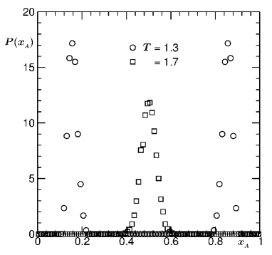
Figure 1: Plots of the concentration probability distribution, $P(x_{{}_{A}})$, vs $x_{{}_{A}}$, for two different temperatures. The system size considered was $L=10$.

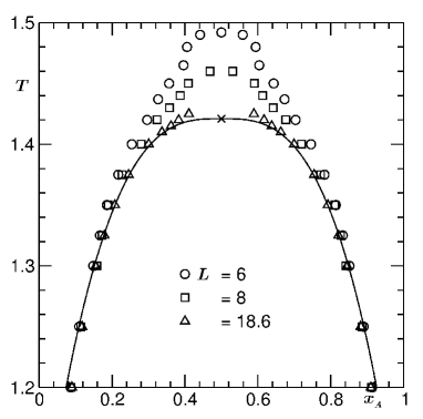
Figure 2: Coexistence curves for the binary LJ system in $T-x_{{}_{A}}$ plane, for three different system sizes. The continuous line is a fit to the largest system data, with the form $m\sim\epsilon^{\beta}$, by taking points in the region unaffected by finite size of the system and fixing $\beta$ to $0.325$. The cross corresponds to the coordinate $(x_{{}_{A}},T)\equiv(1/2,1.421)$, the thermodynamic critical point.

A standard practice in the computer simulations of dynamics is to calculate transport coefficient, $X$, using the Green-Kubo (GK) relation hansen

$$X(t)=\int_{0}^{t}dt^{\prime}A(t^{\prime}),~{}~{}A(t^{\prime})=\langle C(t^{\prime})C(0)\rangle,$$ (14)

where $C$, e.g., for self-diffusion coefficient ($D$) is proportional to the individual particle velocity. Noting the definition of mutual diffusivity das3 ; das4

$$D_{{}_{AB}}=\frac{{\mathscr{L}}}{\chi},$$ (15)

one identifies $\mathscr{L}$, the Onsager coefficient, as the pure dynamic quantity, the GK relation for which is hansen

$${\mathscr{L}}(t)=\left(\frac{t_{{}_{0}}\varepsilon}{k_{{}_{B}}NT\sigma^{2}}\right)\int_{0}^{t}dt^{\prime}\langle{J_{{}_{AB}}^{x}}(t^{\prime}){J_{{}_{AB}}^{x}}(0)\rangle,$$ (16)

where $\vec{J}_{{}_{AB}}$, the concentration current, is defined as hansen

$${\vec{J}}_{{}_{AB}}(t)={{x_{{}_{B}}}{\sum}_{i=1}^{N_{{}_{A}}}{\vec{v}_{{}_{i,A}}}(t)}-{{x_{{}_{A}}}{\sum}_{i=1}^{N_{{}_{B}}}{\vec{v}_{{}_{i,B}}}(t)},~{}~{}$$ (17)

with ${\vec{v}}_{{}_{i,\alpha}}$ being the velocity of particle $i$ of species $\alpha$. Note that $J_{{}_{AB}}^{x}$ is the $x$-component of $\vec{J}_{{}_{AB}}$. The true values of these transport coefficients will be obtained in the limit $t\rightarrow\infty$. Instead of dealing with the velocities of all the particles, as seen in Eq. (17), to facilitate faster calculation, one can use the momentum conservation to work with only one species. This will, in particular, be of advantage for very off-critical composition. This fact will be used in the derivation of the Einstein formula below.

Corresponding relations for viscosities can be written as hansen

$$Y(t)={\left(\frac{t_{{}_{0}}^{3}\varepsilon}{VT\sigma m_{p}^{2}}\right)\int_{0}^{t}dt^{\prime}\langle{P^{\prime}_{ab}}(t^{\prime}){P^{\prime}_{ab}}(0)\rangle},$$ (18)

where $a,b\in[x,y,z]$ and $P^{\prime}_{ab}$ are related to the elements $P_{ab}$, of stress tensor, having the expression

$$P_{ab}=\sum_{i=1}^{N}\Big{[}m_{p}{v_{i}^{a}}{v_{i}^{b}}+{\frac{1}{2}}\sum_{j}^{{}^{\prime}}{(a_{{}_{i}}-a_{{}_{j}})F_{j}^{b}}\Big{]}.$$ (19)

Note that in Eq. (19) $F_{j}^{b}$ is the $b-$component of the force acting on particle $j$ due to the others, $a_{{}_{i}}$ is the $a-$component of Cartesian coordinate of particle $i$ and similarly, $v_{i}^{a}$ is the $a-$component of the velocity of particle $i$. For $a=b$, one has $P=\langle P_{aa}\rangle$. In that case $P^{\prime}_{aa}=P_{aa}-P$ and allen

$$Y=\zeta+\frac{4}{3}\eta,$$ (20)

with $\eta$ being calculated from the correlator of the off-diagonal elements with $P^{\prime}_{ab}=P_{ab}$.

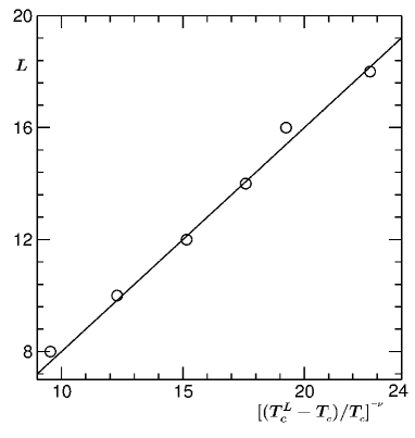
Figure 3: Plot of $L$ vs $[(T_{c}^{L}-T_{{}_{c}})/T_{{}_{c}}]^{-\nu}$. See text for the definition of $T_{c}^{L}$. The value of $\nu$ was fixed to $0.63$.

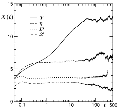
Figure 4: Plots of $Y(t)$, $\mathscr{L}(t)$, $\eta(t)$ and $D(t)$, for $L=10$. Results for $\mathscr{L}$, $\eta$ and $D$ were multiplied by suitable factors to make them visible on the range of ordinate. All results correspond to $x_{{}_{A}}=x_{{}_{A}}^{c}$ and $T=2.5$.

Because of the strong divergence that $\zeta$ exhibits, extremely long simulation runs are necessary, particularly in close vicinity of the critical point. For MD runs in microcanonical ensemble, which is needed for hydrodynamics, it is extremely difficult to keep the system temperature within acceptable fluctuation for long. Further, when the simulations are long, additional difficulty may appear in the accurate estimation of average pressure, due to truncation error, which is needed for the correlator in Eq. (18). Essentially one requires long runs and averaging over huge number of independent initial configurations.

Instead of the GK relation, self-diffusivity is often calculated from the mean-squared-displacement (MSD), referred to as the Einstein relation, as hansen

$$D=\lim_{t\rightarrow\infty}\frac{\langle|{\vec{r}}_{{}_{i}}(t)-{\vec{r}}_{{}_{i}}(0)|^{2}\rangle}{6t},$$ (21)

which is a consequence of Fick’s law of diffusion and provides information about random character of walk or displacement in the linear regime in long $t$ limit. As opposed to $D$, which is a single particle property, $D_{{}_{AB}}$ is related to the collective dynamics of the system. More precisely, it corresponds to the displacement of the centre of mass (CM) of one of the species which will be clear from its expression hansen ; das5 analogous to Eq. (21).

For a system with zero total linear momentum

$${\sum}_{i=1}^{N_{{}_{A}}}{\vec{v}_{{}_{i,A}}}(t)=-{\sum}_{i=1}^{N_{{}_{B}}}{\vec{v}_{{}_{i,B}}}(t).$$ (22)

Defining the CM position $\vec{R}_{{}_{\alpha}}$ and CM velocity $\vec{V}_{{}_{\alpha}}$ of species $\alpha$ as

$${\vec{R}_{{}_{\alpha}}}(t)=\frac{1}{N_{{}_{\alpha}}}{\sum}_{i=1}^{N_{{}_{\alpha}}}{\vec{r}_{{}_{i,\alpha}}}(t),$$

$$~{}~{}{\vec{V}_{{}_{\alpha}}}(t)=\frac{1}{N_{{}_{\alpha}}}{\sum}_{i=1}^{N_{{}_{\alpha}}}{\vec{v}_{{}_{i,\alpha}}}(t),$$ (23)

one writes the momentum conservation relation as

$${N_{{}_{A}}}{\vec{V}_{{}_{A}}}(t)=-{N_{{}_{B}}}{\vec{V}_{{}_{B}}}(t).$$ (24)

From Eqs. (17), (23) and (24), one obtains

$${\vec{J}}_{{}_{AB}}(t)={N_{{}_{A}}}{\vec{V}_{{}_{A}}}(t),$$ (25)

which leads to

$${\mathscr{L}}(t)=\left(\frac{{t_{{}_{0}}}N_{A}^{2}\varepsilon}{k_{{}_{B}}NT\sigma^{2}}\right)\int_{0}^{t}dt^{\prime}\langle{V_{A}^{x}}(t^{\prime}){V_{A}^{x}}(0)\rangle.$$ (26)

Using

$$\vec{R}_{{}_{A}}(t)-\vec{R}_{{}_{A}}(0)=\int_{0}^{t}dt^{\prime}\vec{V}_{{}_{A}}(t^{\prime})$$ (27)

in Eq. (26), one gets hansen ; das5

$${\mathscr{L}}(t)=\left(\frac{{t_{{}_{0}}}N_{A}^{2}\varepsilon}{2k_{{}_{B}}tNT\sigma^{2}}\right)\langle|R_{{}_{A}}^{x}(t)-R_{{}_{A}}^{x}(0)|^{2}\rangle.$$ (28)

A difference in the numerical factor ($2$ instead of $6$) between Eqs. (28) and (21) is due to the fact that here we are working with only one Cartesian component. In addition to the advantage of dealing with only one species in the system, Eq. (28) provides data storage benefit, since one does not need to use data at infinitesimal intervals. This is useful for heavy computations like in critical dynamics.

Similar expressions for viscosities can also be obtained hansen , e.g., $\eta$ can be written as

$$\eta(t)=\left(\frac{t_{{}_{0}}^{3}\varepsilon}{2k_{{}_{B}}tNT\sigma m_{p}^{2}}\right)\langle|Q_{{}_{xy}}(t)-Q_{{}_{xy}}(0)|^{2}\rangle,$$ (29)

where the generalized displacement $Q_{xy}$ has the formula hansen

$$Q_{{}_{xy}}(t)=\sum_{i=1}^{N}{x_{{}_{i}}(t)v_{i}^{y}(t)}.$$ (30)

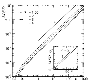
Figure 5: Mean squared displacements corresponding to $\mathscr{L}$ are plotted for different temperatures, at $x_{{}_{A}}=x_{{}_{A}}^{c}$, vs $t$. The inset shows corresponding result for $\eta$.

In order to relate the GK and Einstein relations, one needs to identify the relevant current, which, for self-diffusivity is the tagged particle velocity, for mutual diffusivity is the CM velocity of one of the species. The GK relation is the integration of the autocorrelation of this current. Corresponding displacement variable provides the Einstein relation. For shear viscosity the relevant quantity is the transverse current fluctuation hansen $\frac{im_{p}}{k}\sum_{j=1}^{N}v_{j}i^{x}(t)exp[-i{\vec{k}}.{\vec{r}}_{{}_{j}}]$ ($k$ being the wave vector). The time derivative of this provides the elements of stress tensor and in the small $k$ limit, after imposing the total momentum conservation, one obtains Eq. (30).

In this section we do not describe the methods of analysis of the simulation results. We will discuss them in the next section while presenting the results. Before proceeding to show the results, we set the values of $k_{{}_{B}}$, $m_{p}$, $\sigma$, $\varepsilon$ to unity and so of $t_{{}_{0}}$.

III Results

We start by showing plots of $P(x_{{}_{A}})$ vs $x_{{}_{A}}$ in Fig. 1, from SGMC simulations, for two different temperatures. It is clear from this figure that $T_{{}_{c}}$ lies in between these two temperatures. At very low $T$, it is possible that the system gets stuck in one of the phases because of high energy barrier coming from interfacial tension. In that case it is advisable to carry out biased simulations, e.g., successive umbrella sampling virnau , to access the whole configuration space. On the other hand, one can use the model symmetry, if present, to identify the other phase. Indeed, in this figure we have used the fact

$$P(x_{{}_{A}})=P(1-x_{{}_{A}}),$$ (31)

because of which the data looks perfectly symmetric around $x_{{}_{A}}=1/2$.

In Fig. 2 we show the coexistence curves in $T$ vs $x_{{}_{A}}$ plane for different system sizes. At very low temperature, there is a nice agreement of data from all the sizes. With the increase of temperature, one observes pronounced disagreement among various data sets, giving rise to strong system size dependence of the critical temperature. The value of $L-$dependent critical temperature Yethiraj , $T_{c}^{L}$, is estimated to be the temperature at which there is a crossover from two-peak to single peak structure of $P(x_{{}_{A}})$. An initial guess for this can be facilitated by fitting the negative of the log of the low temperature distribution to Landau free energy form plischke with symmetric double well having temperature dependent coefficients. Note that a true critical temperature is meaningful only in the limit $L\rightarrow\infty$. However, identification of $T_{c}^{L}$s will be helpful to obtain quantitative information on the critical singularities, in thermodynamic limit, from finite systems.

The continuous line in Fig. 2 is obtained from the fit to the $L=18.6$ data in the finite-size unaffected region by fixing $\beta$ to $0.325$ and using $T_{{}_{c}}$ as an adjustable parameter. This provides $T_{{}_{c}}\simeq 1.421$. Note here that in an earlier work das3 ; das4 , from the crossing of Binder parameter binder data from different values of $L$, $T_{{}_{c}}$ was obtained to be $1.423$. In that work no finite-size scaling analysis for Binder parameter crossing was done. However, in the same work, finite-size scaling analysis of the susceptibility data showed slightly better consistency with $T_{{}_{c}}=1.421$, when $T_{{}_{c}}$ was used as an adjustable parameter in data collapse experiment. So, we adopt this value for the rest of this paper.

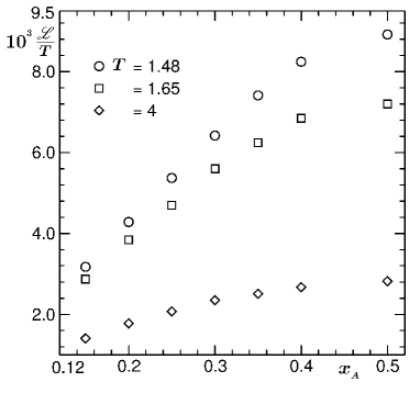
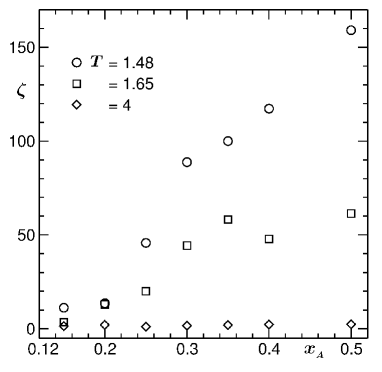
Figure 6: (a) Plots of ${\mathscr{L}}/{T}$ as a function of $x_{{}_{A}}$, for three different temperatures. All results are from same system size with $L=10$. (b) Same as (a), but for $\zeta$.

Considering the fact that at $T_{c}^{L}$, $\xi$ assumes the value $L$, one can write down

$$L\sim\Big{(}\frac{T_{c}^{L}-T_{{}_{c}}}{T_{{}_{c}}}\Big{)}^{-\nu}.$$ (32)

In Fig. 3 we have plotted $L$ vs $((T_{c}^{L}-T_{c})/T_{c})^{-\nu}$ by fixing $\nu$ to its Ising value and $T_{{}_{c}}$ to $1.421$. Consistency of the simulation data with the solid straight line confirms Eq. (32). We will use these values of $T_{c}^{L}$ later in the finite-size scaling analysis of transport coefficients. The random scatter seen in these data on both sides of the straight line is much smaller than the temperature fluctuation in NVE ensemble MD simulations.

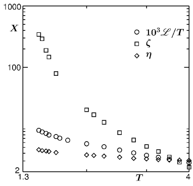
Figure 7: Plots of ${\mathscr{L}}/{T}$, $\eta$ and $\zeta$ as a function of $T$, at $x_{{}_{A}}=x_{{}_{A}}^{c}$. All results correspond to $L=10$.

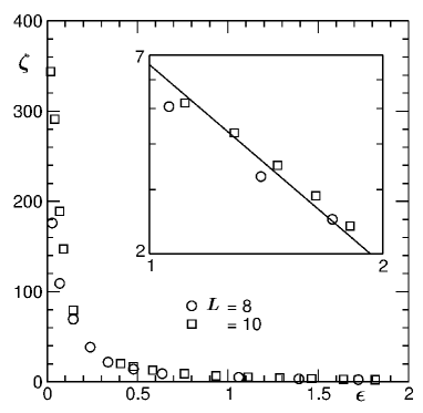
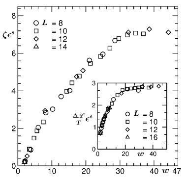
Figure 8: (a) Plots of $\zeta$ vs $\epsilon$, along $x_{{}_{A}}=x_{{}_{A}}^{c}$, for two different system sizes. The solid line in the inset has a power-law divergence with exponent $1.82$. (b) Finite-size scaling plot for $\zeta$, viz., $\zeta\epsilon^{s}$ vs $w$, with $s=\nu x_{{}_{\zeta}}=1.82$. Data from four different $L$ values are used. Inset: Same as the main figure, but for $\mathscr{L}$. In this case $s$ has a value $0.567$.

On dynamics, we start by demonstrating how various quantities were obtained. In Fig. 4 we show the integrations of the autocorrelations for $\mathscr{L}$, $\eta$, $Y$, and $D$ as functions of time. These quantities were estimated from the pleatue region. All these results correspond to $x_{{}_{A}}=1/2$, $T=2.5$ and $L=10$. The relaxation of the correlators for different quantities at different times is indicative of varying critical enhancement. The result for $D$ appears smoother than the others. This is due to the difference between collective system property and individual particle property. In the latter case, there is scope of self averaging over all the particles in the system. The lack of this for collective properties make the estimation of these quantities significantly difficult, particularly in the close vicinity of critical point where relaxation time diverges.

In Fig. 5 we show the MSDs for $\mathscr{L}$ at different temperatures along $x_{{}_{A}}^{c}$. The corresponding result for $\eta$ is shown in the inset. At late time nice linear behavior is seen, implying Einsteinian diffusion of relevant variables. From the time derivative of these results, in long time limit, the transport coefficients can be estimated which, we have checked, are in good agreement with the estimates from Fig. 4.

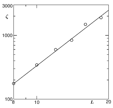
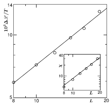
Figure 9: (a) Plot of $\zeta$, calculated at $T_{c}^{L}$s, as a function of $L$. The solid line represents power-law with exponent $2.89$. (b) Same as (a), but for ${\Delta{\mathscr{L}}}/{T}$. Here the solid line has exponent $0.9$. The inset shows same exercise for $\chi$.

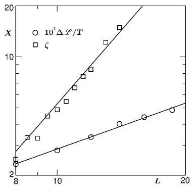
Figure 10: Same as Fig. 10, but the quantities were calculated at $T_{c}^{L}(f)$ with $f=65$.

In Fig. 6(a) we show the plots of ${\mathscr{L}}/{T}$ as a function of $x_{{}_{A}}$, for three different temperatures. Note that we have confined ourselves to $x_{{}_{A}}\leq 0.5$. The result will be mirror image on the other side because of the symmetry of the model. The reason for choosing ${\mathscr{L}}/{T}$, instead of only $\mathscr{L}$, is clear from Eqs. (2), (6) and (15) which suggest

$$\frac{\mathscr{L}}{T}=Q\epsilon^{-\nu_{{}_{\lambda}}};~{}\nu_{{}_{\lambda}}=0.567,$$ (33)

where $Q$ is a critical amplitude. Enhancement of ${\mathscr{L}}/{T}$ with the approach towards the critical composition is clear which is more and more prominent for temperatures closer to the critical value. Interestingly, this enhancement even for $T=4$ is significant and perhaps signals a very wide critical range. In Fig. 6(b) we present analogous results for $\zeta$. Qualitative behavior of the data here is same as Fig. 6(a), but rise in $\zeta$ as a function of $x_{{}_{A}}$ as well as $T$ appears much stronger than $\mathscr{L}$, implying a larger value of critical exponent for $\zeta$. This is, of course, the prediction of theories which we will quantify in this work. Note that an apparently flat look of data for $T=4$ in this case is due to the large scale of the ordinate.

A comparative picture of the critical enhancement of various transport coefficients, along the critical concentration, is shown in Fig. 7. Here, in addition to $\zeta$ and $\mathscr{L}$, we have included $\eta$ also. Data for $\mathscr{L}$ has been multiplied by $1000$. It is clearly seen that the enhancement of $\zeta$ is much stronger than $\mathscr{L}$. On the other hand, data for $\eta$ appears rather insensitive to the approach to criticality. This is consistent with the prediction of a very small value for the corresponding critical exponent. Considering this and combining with the fact that temperature fluctuation in NVE ensemble is rather high, we do not aim to proceed further with detailed analysis for the critical behavior of $\eta$. For $D$, on the other hand, there is no theoretical expectation for critical enhancement which we will demonstrate towards the end of the paper.

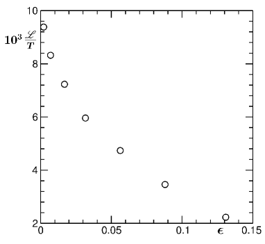
Figure 11: Plot of ${\mathscr{L}}/{T}$ as a function of $\epsilon$, for $T<T_{{}_{c}}$, along the B-rich branch of the coexistence curve. The system size was chosen to be $L=10$.

In Fig. 8(a) we present results for $\zeta$ vs $\epsilon$, along $x_{{}_{A}}=x_{{}_{A}}^{c}$, for two different system sizes. The discrepancy between the two data sets for smaller values of $\epsilon$ is due to finite-size effects which appear rather strong that can be appreciated from the fact that results from the two systems agree only at very large value of $\epsilon$. In the latter region, shown on double-log scale in the inset, the data are consistent with the solid line which has a power-law with theoretical exponent $\nu x_{{}_{\zeta}}=1.82$. To confirm this critical exponent further, we take help of the following finite-size scaling method.

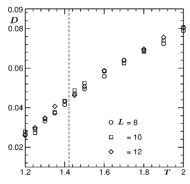
Figure 12: Plot of self-diffusivity $D$, for species $A$, as a function of $T$. Results for few different system sizes are shown. For $T<T_{{}_{c}}$, we have chosen the B-rich branch of the coexistence curve. The vertical dashed line represents the value of $T_{{}_{c}}$.

Since fluctuation can never become truly critical in a finite system, the enhancement

$$X\sim\epsilon^{-s}$$ (34)

gets suppressed there. Nevertheless, it is possible to obtain information about the exponent $s$ and other relevant quantities in critical phenomena via appropriate scaling analysis landau ; fisher2 involving finite values of $L$. For $L<\infty$, one introduces a finite-size scaling function $Z$ to write

$$X=Z(w)\epsilon^{-s},$$ (35)

where $Z$ is independent of system size and depends upon the dimensionless variable $w=L/\xi$, $\xi$ having the thermodynamic limit behavior. Thus, in a plot of $X\epsilon^{s}$ vs $w$, data for different values of $L$ will collapse onto a master curve, of course, if the exponent $s$ is appropriately chosen. For far away from $T_{{}_{c}}$, where $\xi<<L$, one does not expect finite-size effects. In that limit, $Z(w)$ will be a constant equal to the critical amplitude of the quantity under study. For $T$ very close to $T_{{}_{c}}$, finite-size effects will certainly become important, thus $X$ will tend towards a constant, allowing one to write

$$Z(w)\sim w^{s/\nu}\sim\epsilon^{s}.$$ (36)

We do an exercise along the line described above, in the main frame of Fig. 8(b), for $\zeta$. Here the value of $s$ was set to $1.82$ which provides excellent collapse of data from many different system sizes. Flat portion, in this figure, in the large $w$ limit, provides the value of critical amplitude to be $\simeq 7.07$.

Similar analysis for $\mathscr{L}$ was done previously das3 ; das4 . For the sake of completeness, we show it in the inset of Fig. 8(b), this time with more data points. Previously, strong background in $\mathscr{L}$, coming from small length fluctuations, was observed das3 ; das4 , so that in the critical vicinity one should write

$${\mathscr{L}}={\mathscr{L}}_{b}+\Delta{\mathscr{L}},$$ (37)

where ${\mathscr{L}}_{b}$ and $\Delta{\mathscr{L}}$ are respectively the background and critical contributions. To obtain information about the critical exponent, in such cases, one needs to subtract the value of ${\mathscr{L}}_{b}$ appropriately. This was done by using ${\mathscr{L}}_{b}$ as an adjustable parameter in the finite-size data collapse experiment by fixing $x_{{}_{\lambda}}$ to $0.567$. The value that provides best collapse is das3 ; das4 ${\mathscr{L}}_{b}\simeq 3.3\times 10^{-3}$, giving $Q\simeq 2.8\times 10^{-3}$ which can be appreciated from the plot presented in the inset. In the following we will use this number for ${\mathscr{L}}_{b}$ and check via other type of analysis if the exponent value $x_{{}_{\lambda}}=0.567$ is correct which was fixed in this case.

Next, we exploit the scaling behavior of $T_{c}^{L}$ with $L$, demonstrated in Fig. 3, to obtain further confirmation on the critical divergences of these quantities. By observing Eq. (32), while dealing with data calculated at $T_{c}^{L}$s, one can write down

$$X\sim L^{-s/\nu}.$$ (38)

In Fig. 9(a) we plot $\zeta$ vs $L$ on a double-log scale using data at $T_{c}^{L}$s. The consistency of the simulation data with the solid line, bearing the theoretical exponent $2.89$, is clearly visible. Here note that for a binary fluid the value of the exponent $x_{{}_{\zeta}}$ was pointed out jkb1 ; jkb2 to be closer to $3$. This difference, however, is difficult to confirm from the quality of our simulation data. In Fig. 9(b), we show ${\Delta\mathscr{L}}/{T}$ vs $L$, again on double-log scale. Here also the data are consistent with the theory, represented by the solid line. This, in addition, confirms the choice of ${\mathscr{L}}_{b}$, quoted earlier. In the inset of Fig. 9(b) we do same exercise for $\chi$ demonstrating consistency with theory, thus confirming that $x_{{}_{D}}=1.07$.

Starting from $T_{c}^{L}$, one can define effective critical temperature as das1 ; roy1

$$T_{c}^{L}(f)=T_{{}_{c}}+f(T_{c}^{L}-T_{{}_{c}}),$$ (39)

which, for $f=0$, is the thermodynamic critical point and for $f=1$, is just $T_{c}^{L}$. Scaling of $T_{c}^{L}(f)-T_{{}_{c}}$, for any arbitrary value of $f$, with $L$, should be same as Eq. (32). Usefulness of such effective critical temperature can be understood as follows. For significantly large values of $L$, if it does not become possible to calculate a quantity at $T_{c}^{L}$, which indeed is true for transport properties with strong critical enhancements, one can choose a suitably large value of $f$ to avoid computational effort, of course, if the critical range is extended that far. In this paper, we will use a rather large value of $f$, to obtain information on the critical range.

In Fig. 10 we show $\zeta$ as well as ${\Delta\mathscr{L}}/{T}$ as functions of $L$, with quantities calculated at $T_{c}^{L}(65)$. The linear looks of both the data sets on a log-log scale are indicative of power-law behaviors. The solid lines there have corresponding theoretical exponents. The temperatures included in this figure, lie in the range $[1.91,3.87]$. Nevertheless, the consistency of the simulation results with theory confirm that the critical range for this model is rather large, a hint of this was already obtained from Fig. 8. For a binary fluid it is expected that the critical range will be wider than a vapor-liquid transition. However, the range we see in this work is very high which could possibly be attributed to the symmetry of the model.

In Fig. 11 we show ${\mathscr{L}}/{T}$ as a function of $\epsilon$, for temperatures below $T_{{}_{c}}$, for $L=10$, calculated at state points along the B-rich branch of the coexistence curve. Enhancement of the quantity with the increase of temperature is clearly visible. Due to lack of data from different system sizes we do not aim to quantify the exponent in this case. Note that the background contribution below $T_{{}_{c}}$ need not be the same as above. Also, while doing finite-size scaling exercise, one needs to consider the finite-size effects in the coexistence curve as well, as seen in Fig. 2. All these put together, it is a substantial task which we leave out for a future work. Nevertheless, the information provided in Fig. 11 (as well as in Fig. 12) is expected to be important in other studies. Noting the simplicity as well as reasonably realistic nature, the model is useful in the understanding of hydrodynamic effects in kinetics of phase separation. For quantitative understanding of the latter, one requires information about various transport coefficients for coexistence composition.

Finally, in Fig. 12 we present the self-diffusion coefficient, $D$, for species $A$, at temperatures above and below $T_{{}_{c}}$. We have included results from few different system sizes. No systematic system size dependence is visible. This, combined with the overall nature of data, do not suggest any critical singularity for this quantity.

IV Conclusion

In summary, we have studied phase behavior and dynamics in a symmetric binary Lennard-Jones model exhibiting liquid-liquid transition. The phase diagram was studied via Monte Carlo simulations in a semi-grandcanonical ensemble landau whereas we have used molecular dynamics simulations frenkel in the microcanonical ensemble to obtain information on dynamics.

Various transport properties, viz., self and mutual diffusivities, shear and bulk viscosities were calculated using Green-Kubo as well as Einstein relations hansen . We have explored a wide range of state points on and around the coexistence curve. Particular focus was on the understanding of critical singularities.

It is observed that the self diffusivity is insensitive to the critical point and shear viscosity exhibits only weak critical enhancement. The critical behaviors of mutual diffusivity as well as bulk viscosity were quantified via various finite-size scaling methods. Our results are nicely in agreement with the predictions of mode coupling and dynamic renormalization group theories hohenberg ; ferrell ; olchowy ; onuki1 ; anisimov ; kadanoff ; mistura ; folk ; onuki2 ; hao ; jkb1 ; jkb2 .

Interestingly, critical range for these transport properties appear to be very large. It is not clear to us whether this is due to the symmetry of the model or the particular interatomic potential. This finding is consistent with one meier of the previous studies for a vapor-liquid transition, with Lennard-Jones interaction, where there is no such symmetry.

For bulk viscosity it needs to be seen whether the Lennard-Jones interaction allows for no other background term until the critical enhancement has become of the same order as the shear viscosity. In Ref. [meier ], even though strong enhancement far away form $T_{c}$ was noticed, no quantitative study with respect to the critical divergence was done. Recently we jia have undertaken independent study of bulk viscosity for vapor-liquid transition, again with Lennard-Jones potential. Quantitative outcome from there can possibly provide some hint along this line.

In future, we will take up the issue of quantifying the exponents below $T_{{}_{c}}$. In that case, it will be interesting to examine the existence of universal amplitude ratios, as is true in static critical phenomena privman . To establish this, one of course needs to study various different models.

References

- (1) P.C. Hohenberg, and B.I. Halperin, Rev. Mod. Phys. 49, 435 (1977).
- (2) R.A. Ferrell, and J.K. Bhattacharjee, Phys. Rev. Lett. 88, 77 (1982).
- (3) G.A. Olchowy and J.V. Sengers, Phys. Rev. Lett. 61, 15 (1988).
- (4) J. Luettmer-Strathmann, J.V. Sengers and G.A. Olchowy, J. Chem. Phys. 103, 7482 (1995).
- (5) A. Onuki, Phys. Rev. E 55, 403 (1997).
- (6) M.A. Anisimov and J.V. Sengers, in Equations of State for Fluids and Fluid Mixtures, ed. J.V. Sengers, R.F. Kayser, C.J. Peters and H.J. White, Jr. (Elsevier, Amsterdam, 2000) p.381.
- (7) A. Onuki, Phase Transition Dynamics (Cambridge University Press, UK, 2002).
- (8) L.P. Kadanoff and J. Swift, Phys. Rev. 166, 89 (1968).
- (9) L. Mistura, Nuovo Cimento 12B, 35 (1972); J. Chem.Phys. 62, 4571 (1975).
- (10) R. Folk and G. Moser, Phys. Rev. Lett. 75, 2706 (1995).
- (11) H.C. Burstyn and J.V. Sengers, Phys. Rev. Lett. 45, 259 (1980).
- (12) H.C. Burstyn and J.V. Sengers, Phys. Rev. A 25, 448 (1982).
- (13) H. Hao, R.A. Ferrell, and J.K. Bhattacharjee, Phys. Rev. E. 71, 021201 (2005).
- (14) J.K. Bhattacharjee, I. Iwanowski and U. Kaatze, J. Chem. Phys. 131, 174502 (2009).
- (15) J.K. Bhattacharjee, U. Kaatze and S.Z. Mirzaev, Rep. Progr. Phys. 73, 066601 (2010).
- (16) J.V. Sengers and J.G. Shanks, J.Stat. Phys. 137, 857 (2009).
- (17) G. Pérez-Sánchez, P. Lasada-Péréz, C.A. Cerdeiriña, J.V. Sengers and M.A. Anisimov, J. Chem. Phys. 132, 154502 (2010).
- (18) M.E. Fisher and G. Orkoulas, Phys. Rev. Lett. 85, 696 (2000).
- (19) E. Luijten, M.E. Fisher, and A.Z. Panagiotopoulos, Phys. Rev. Lett. 88, 185701 (2002).
- (20) Y.C. Kim and M.E. Fisher, Phys. Rev. Lett. 92, 185703 (2004).
- (21) D.J. Ashton, N.B. Wilding and P. Sollich, J. Chem. Phys. 132, 074111 (2010).
- (22) S.K. Das, Y.C. Kim and M.E. Fisher, Phys. Rev. Lett. 107, 215701 (2011).
- (23) K.A. Gillis, I.I. Shinder and M.R. Moldover, Phys. Rev. E 72, 051201 (2005).
- (24) K.A. Gillis, I.I. Shinder and M.R. Moldover, Phys. Rev. Lett. 97, 104502 (2006).
- (25) S.K. Das, J. Horbach and K. Binder, Phase Transitions 77, 823 (2004).
- (26) K. Meier, A. Laesecke and S. Kabelac, J. Chem. Phys. 122, 014513 (2005).
- (27) G. Salin and D. Gilles, J. Phys. A: Math. Gen. 39, 4517 (2006).
- (28) K. Dyer, B.M. Pettitt and G. Stell, J. Chem. Phys. 126,034501 (2007).
- (29) S.K. Das, M.E. Fisher, J.V. Sengers, J. Horbach, and K. Binder, Phys. Rev. Lett. 97, 025702 (2006).
- (30) S.K. Das, J. Horbach, K. Binder, M.E. Fisher and J.V. Sengers, J. Chem. Phys. 125, 024506 (2006).
- (31) A. Chen, E.H. Chinowitz, S.De and Y. Shapir, Phys. Rev. Lett. 95, 255701 (2005).
- (32) M. Gross and F. Varnick, Phys. Rev. E 85, 056707 (2012).
- (33) J.W. Mutoru, W. Smith, C.S. O’Hern and A. Firozabadi, J. Chem. Phys. 138, 024317 (2013).
- (34) T. Fang, L. Wang, C.X. Peng and Y. Qi, J. Phys. Condensed Matter 24, 505103 (2012).
- (35) P. Kumar and H.E. Stanley, J. Phys. Chem. B 115, 14269 (2011).
- (36) A.J. Bray, Adv. Phys. 51, 481 (2002).
- (37) H. Furukawa, Phys. Rev. A 36, 2288 (1987).
- (38) J. Zinn-Justin, Phys. Repts. 344, 159 (2001).
- (39) D.P. Landau and K. Binder, A Guide to Monte Carlo Simulations in Statistical Physics, 3rd Edition (Cambridge University Press, Cambridge, 2009).
- (40) M.E. Fisher in Critical Phenomena, edited by M.S. Green (Academic Press, London, 1971) p.1.
- (41) A. Pelissetto and E. Vicari, Phys. Repts. 368, 549 (2002).
- (42) T.M. Squires and J.F. Brady, Phys. Fluids 17, 073101 (2005).
- (43) J.-P. Hansen and I.R. McDonald, Theory of Simple Liquids (Academic Press, London, 2008).
- (44) S. Roy and S.K. Das, Europhys. Lett. 94, 36001 (2011).
- (45) D. Frenkel and B. Smit, Understanding Molecular Simulations: From Algorithm to Applications (Academic Press, San Diego, 2002).
- (46) M.P. Allen and D.J. Tildesley, Computer Simulations of Liquids (Clarendon, Oxford, 1987).
- (47) D.C. Rapaport, The Art of Molecular Dynamics Simulations (Cambridge University Press, Cambridge, UK, 2004).
- (48) J. Horbach, S.K. Das, A. Griesche, M.-P. Macht, G. Frohberg and A. Meyer, Phys. Rev. B, 75, 174304 (2007).
- (49) P. Virnau and M. Müller, J. Chem. Phys. 120, 10925 (2004).
- (50) K. Jagannathan and A. Yethiraj, Phys. Rev. Lett 93, 015701 (2004).
- (51) M. Plischke and B. Bergersen, Equilibrium Statictical Mechanics (World Scientific, Singapore, 2006).
- (52) K. Binder, Z. Phys. B: Condens. Matter 43, 119 (1981).
- (53) J. Midya and S.K. Das, work under progress.
- (54) V. Privman, P.C. Hohenberg and A. Aharony, in Phase Transitions and Critical Phenomena, edited by C. Domb and J.L. Lebowitz, vol. 14, Chap. 1, Academic Press, New York, 1991.