Finite-size Scaling Study of Shear Viscosity Anomaly at Liquid-Liquid Criticality

Abstract

We study equilibrium dynamics of a symmetrical binary Lennard-Jones fluid mixture near its consolute criticality. Molecular dynamics simulation results for shear viscosity, $\eta$, from microcanonical ensemble are compared with those from canonical ensemble with various thermostats. It is observed that Nosé-Hoover thermostat is a good candidate for this purpose and so, is adopted for the quantification of critical singularity of $\eta$, to avoid temperature fluctuation (or even drift) that is often encountered in microcanonical simulations. Via finite-size scaling analysis of our simulation data, thus obtained, we have been able to quantify even the weakest anomaly, of all transport properties, that shear viscosity exhibits and confirm the corresponding theoretical prediction.

I Introduction

Knowledge of the behaviors of equilibrium transport properties, with the variation of various thermodynamic parameters, is crucial even to the understanding of nonequilibrium dynamics onuki1 ; bray . In computer simulations, reliable calculations of collective transport properties onuki1 ; hansen , e.g., shear ($\eta$) and bulk ($\zeta$) viscosities, thermal diffusivity ($D_{T}$), mutual diffusivity ($D_{AB}$) in a ($A+B$) binary mixture, etc., are extremely difficult due to lack of self averaging onuki1 ; hansen ; allen . Simulation studies of dynamic critical phenomena, because of this reason, have started only recently yeth1 ; yeth2 ; chen ; das2006 ; dasjcp2006 ; roy1 ; roy2 .

In the vicinity of a critical point, various static and dynamic properties exhibit power-law singularities onuki1 ; zinn ; hohenberg . E.g., in static critical phenomena, the correlation length ($\xi$), order parameter ($m$) and susceptibility ($\chi$) behave as onuki1 ; zinn

$$\xi\approx\xi_{0}^{\pm}\epsilon^{-\nu},~{}m\approx\hat{B}\epsilon^{\beta},~{}\chi\approx\Gamma^{\pm}\epsilon^{-\gamma};~{}\epsilon=\frac{|T-T_{c}|}{T_{c}},$$ (1)

where $T$ is the temperature, $T_{c}$ being its value at the critical point. The superscripts $\pm$ on the amplitudes $\xi_{0}$ and $\Gamma$ signify singularities irrespective of which side of $T_{c}$ one approaches it. In dynamics onuki1 ; hohenberg ; kadanoff ; anisimov ; onuki2 ; olchowy ; folk ; hao ; jkb1 ; jkb2 ; sengers ; burstyn1 ; burstyn2 ; landau , the relaxation time ($\tau$) and the above mentioned transport quantities have the critical behaviors

$$\tau\sim\xi^{z},~{}\eta\sim\xi^{x_{\eta}},~{}\zeta\sim\xi^{x_{\zeta}},~{}D_{T,AB}\sim\xi^{-x_{D}}.$$ (2)

The values of the critical exponents do not depend upon the atomistic details of the systems. In case of static properties, these are even independent of type of transitions, i.e., demixing transitions in binary solids and fluids, vapor-liquid transitions or para- to ferromagnetic transitions will have same values of the exponents, if the system dimensionality and number of order-parameter components are same, alongside inter-particle interactions being of similar range. For short range interactions, with one component order parameter, the universality belongs to the Ising class for which the values of the exponents in space dimension $d=3$ are zinn

$$\nu=0.63,~{}\beta=0.325,~{}\gamma=1.239.$$ (3)

Such universalities exist in dynamics as well, though less robust. E.g., vapor-liquid and liquid-liquid transitions are expected to belong to the same universality hohenberg ; kadanoff ; anisimov ; onuki2 ; olchowy ; folk ; hao ; jkb1 ; jkb2 ; sengers ; burstyn1 ; burstyn2 ; landau , with $z\simeq 3.068$, which is different from that of a para- to ferromagnetic transition landau , having $z\simeq 2.15$. This difference is due to the nonconservation of order parameter in the ferromagnetic case. In addition to standard finite-size effects, encountered in static critical phenomena, the high value of $z$, particularly for fluid criticality, makes the study of dynamic critical phenomena significantly more difficult. This phenomenon, referred to as the critical slowing down, can be appreciated from the fact that the relaxation time at criticality, where $\xi$ scales with the system size $L$, diverges as landau

$$\tau\sim L^{z}.$$ (4)

The values of the other dynamic exponents in $d=3$ fluid universality class are onuki1 ; hao ; jkb1 ; jkb2 ; olchowy

$$x_{\eta}\simeq 0.068,~{}x_{\zeta}\simeq 2.89,~{}x_{D}\simeq 1.068,$$ (5)

for $x_{\zeta}$ the value being slightly higher for a liquid-liquid transition. For the latter, singularities of $D_{AB}$ and $\zeta$ were recently verified via molecular dynamics (MD) simulations das2006 ; dasjcp2006 ; roy1 ; roy2 . However, quality of data were not appropriate enough to draw a conclusion on the anomaly of $\eta$, because of the tiny value of $x_{\eta}$.

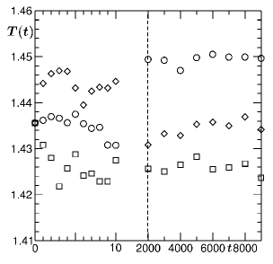
Figure 1: Plots of temperature as a function of time, during microcanonical molecular dynamics runs of the binary Lennard-Jones mixture. The system size is $L=14$. Before each of these runs, the system was appropriately equilibrated for long enough time via Monte Carlo runs in canonical ensemble and further, thermalized via molecular dynamics runs with Andersen thermostat. The initial temperature was set to a value reasonably close to the critical one.

Fluid transport properties, via MD simulations allen ; frenkel ; rapaport , are traditionally calculated in microcanonical ensemble (constant NVE, $N$ being the total number of particles, $V$ the volume and $E$ energy) where hydrodynamics is ideally satisfied. However, temperature in this ensemble is not perfectly controlled which is nondesirable for the quantification of critical singularity, particularly when expected anomaly is weak. The fluctuation of temperature in NVE ensemble, during MD simulations of our binary fluid model (to be defined soon), is shown in Fig. 1. There we have plotted $T$ as a function of time ($t$) for a few different runs. It is common experience, as seen here, that in long time limit, the value of $T$ settles down to a nondesirable number. For more realistic models (than the one we use here), the temperature drift can be stronger than seen in Fig. 1.

To avoid the above mentioned problem, we have planned to calculate $\eta$ in canonical ensemble as well, with hydrodynamics preserving thermostat. In addition to accurate computation, an objective of the work is to demonstrate that critical dynamics in fluids can be studied in canonical ensemble. The suitable candidates for this purpose are Nosé-Hoover thermostat (NHT) frenkel , dissipative particle dynamics stoya ; niku , multiparticle collision dynamics gomp , etc. For technical reasons, related to temperature control, we will adopt the NHT for this work. Our simulation data from NHT, when analyzed via finite-size scaling (FSS) landau ; fisher_fss , show excellent agreement with the theoretically predicted singularity, quoted in Eq. (5). As mentioned earlier, this is the first such confirmation of the critical anomaly of shear viscosity.

The rest of the paper is organized as follows. In Section II we discuss the model and methods. Results are presented in Section III. Finally, Section IV concludes the paper with a brief summary.

II Model and Methods

We consider a binary fluid model das2006 ; dasjcp2006 ; roy1 ; roy2 where particles, all of same mass $m$, at continuum positions ${\vec{r}}_{i}$ and ${\vec{r}}_{j}$, interact via the Lennard-Jones (LJ) pair potential

$$u(r=|{\vec{r}}_{i}-{\vec{r}}_{j}|)=4\varepsilon_{{}_{\alpha\beta}}\Big{[}\Big{(}\frac{d_{0}}{r}\Big{)}^{12}-\Big{(}\frac{d_{0}}{r}\Big{)}^{6}\Big{]},$$ (6)

where $d_{0}$ is the particle diameter, same for all, and $\varepsilon_{\alpha\beta}~{}[\alpha,\beta=A,B]$ are the interaction strengths. We set $\varepsilon_{{}_{AA}}=\varepsilon_{{}_{BB}}=2\varepsilon_{{}_{AB}}=\varepsilon$ which, in addition to facilitating phase separation, makes the model perfectly symmetric. For computational benefit, we truncate the potential at an inter-particle distance $r=r_{c}=2.5d_{0}$ and work with the shifted and force-corrected form allen

$$U(r)=u(r)-u(r_{c})-(r-r_{{}_{c}}){\frac{du}{dr}}\Big{|}_{{r}=r_{{}_{c}}}.$$ (7)

The number density of particles $\rho$ ($=N/L^{3}$) was fixed to $1$, a value high enough to avoid any overlap with a vapor-liquid transition.

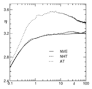
Figure 2: Plot of $\eta(t)$ as a function of $t$ at $T=3.25$. Results from microcanonical MD and canonical MD with NHT and AT are shown. The value of $\eta$ can be obtained from the plataea of these plots.

Static quantities for this model were studied das2006 ; dasjcp2006 ; roy1 ; roy2 via Monte Carlo landau (MC) simulations in semi-grand canonical ensemble landau ; frenkel (SGMC) where, in addition to standard displacement moves, identity switches $A\rightarrow B\rightarrow A$ are also tried. This allows one to record the fluctuations of concentration $x_{\alpha}$ ($=N_{\alpha}/N$, $N_{\alpha}$ being the number of particles of species $\alpha$) of either species and thus distribution $P(x_{\alpha})$. As we will discuss later, this enables estimation of phase diagram, in addition to several other static quantities.

Transport quantities were calculated using the MD simulations in NVE as well as in Canonical ensembles. For the latter we have used NHT as well as Andersen thermostat (AT) frenkel . In AT, to keep the temperature constant, randomly chosen particles are made to collide with a fictitious heat bath, i.e, they are assigned new velocities in accordance with the desired temperature. Thus hydrodynamics is not expected to be preserved by AT. For NHT, we have solved the standard deterministic equations of motion frenkel

$$m_{i}\dot{r_{i}} = p_{i},$$ (8)

$$\dot{p_{i}} = -\frac{\delta U_{i}}{\delta r_{i}}-\Xi p_{i},$$ (9)

$$\dot{\Xi} = \Big{(}\sum_{i=1}^{N}p_{i}^{2}/m_{i}-3N{k_{B}}T\Big{)}/Q,$$ (10)

where $k_{B}$ is the Boltzmann constant, $\Xi$ is a time dependent drag and $Q$ is a constant providing the strength of coupling of the system with the thermostat. The value of $Q$ was set to $1$ and also for $\Xi$ we have started with unity in each MD run. In both the ensembles, Verlet velocity algorithm was used to integrate the equations of motion, with the time step of integration being set to $0.005t_{0}$, where $t_{0}$ ($=\sqrt{md_{0}^{2}/\varepsilon}$) is the LJ time unit.

We computed shear viscosity using the Green-Kubo (GK) and Einstein relations hansen . The GK relation is given by

$$\eta(t)={\left(\frac{t_{{}_{0}}^{3}\varepsilon}{Vd_{0}Tm^{2}}\right)\int_{0}^{t}dt^{\prime}\langle{\sigma_{xy}}(t^{\prime}){\sigma_{xy}}(0)\rangle},~{}~{}~{}$$ (11)

where $\sigma_{xy}$ are the off-diagonal elements of the pressure tensor, computed as

$$\sigma_{xy}(t)=\sum_{i=1}^{N}\Big{[}mv_{ix}v_{jy}+\frac{1}{2}\sum_{j(\neq i)}(x_{i}-x_{j})F_{jy}\Big{]},~{}~{}~{}$$ (12)

with $v_{{}_{ix}}$ being the $x$ component of the velocity of $i$th particle and $F_{jy}$ the $y$ component of force acting on the $j$th particle due to all others. The Einstein formula for the calculation of $\eta$ is

$$\eta(t)=\left(\frac{t_{{}_{0}}^{3}\varepsilon}{2k_{{}_{B}}tVd_{0}Tm^{2}}\right)\langle|Q_{{}_{xy}}(t)-Q_{{}_{xy}}(0)|^{2}\rangle,$$ (13)

where the generalized displacement $Q_{xy}$ has the form hansen

$$Q_{{}_{xy}}(t)=\sum_{i=1}^{N}{x_{{}_{i}}(t)v_{iy}(t)}.$$ (14)

Both Eq. (11) and Eq. (13) provide similar results, but in this paper we present the ones obtained only from the Einstein relation.

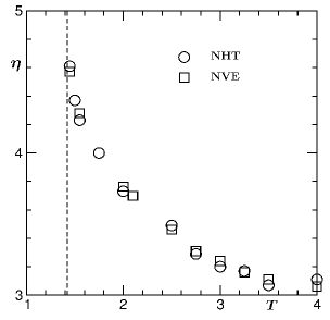
Figure 3: The shear viscosity is plotted as a function of $T$. Results from NVE and NHT calculations are shown. The system size used was $L=10$. The dashed line stands for $T_{c}=1.421$.

All simulations were performed in cubic boxes of volume $V$($=L^{3}$, $L$ being in units of $d_{0}$), with periodic boundary condition in each direction. Results are presented after averaging over multiple initial configurations. For phase behavior, at each temperature, $6$ different initial configurations were averaged over, while this number was from $400$ to $650$, depending on the system size, for shear viscosity. For dynamics we have stuck to the critical composition $x_{\alpha}^{c}=1/2$, the value being set by the symmetry of the model. For the rest of our paper, the values of $m$, $\varepsilon$, $d_{0}$, $t_{0}$ and $k_{B}$ were fixed to unity.

III Results

In Fig. 2 we plot $\eta(t)$ as a function of $t$, obtained via Eq. (13), at $T=3.25$. Results are presented from NVE and NVT ensembles. For the latter, calculations using both NHT and AT are included. It is clearly seen that NHT produces result comparable with NVE ensemble. As discussed, AT does not meet the momentum conservation condition. Deviation of AT result from the others provide further confidence that the matching of NHT and NVE is not accidental. Final values of $\eta$ were obtained from the flat regions in $\eta(t)$ vs $t$ plots.

In Fig. 3 we show the variation of $\eta$ as a function of $T$, for $L=10$. Critical enhancement is visible. Results from NVE and NHT are shown which agree nicely with each other. Being encouraged by the good agreement between them, we adopt the latter for quantification of critical singularity via FSS. At this stage we do not attempt to quantify the critical singularity using these data, fearing finite-size effects. We introduce the FSS method below, via discussion of the phase behavior.

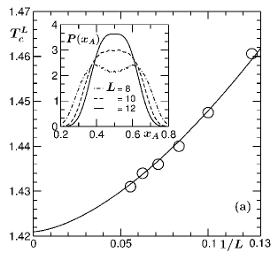
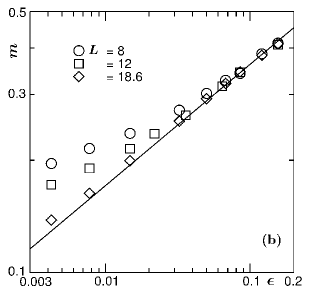
Figure 4: (a) Plot of $T_{c}^{L}$ as a function of $1/L$. The continuous line there is a fit to the scaling form (15). This line meets the ordinate at $T_{c}=1.421$ for $L=\infty$. Inset: Probability distributions $P(x_{A})$ is plotted vs $x_{A}$, for a few different system sizes at $T=1.4475$. (b) Order parameter $m$, defined in Eq. (17), is plotted vs $\epsilon$, on log-log scales, for a few different system sizes, as indicated. The continuous line has Ising critical behavior.

Like all other quantities, phase diagram also suffers from finite-size effects, in the close vicinity of a critical point. For a binary mixture, the demixing phase diagram can be obtained from the SGMC simulations in the following way. The probability distribution $P(x_{\alpha})$ will have a double peak structure below the critical point. The locations of these peaks will provide points for the coexistence curve. Thus, these peaks should merge at the critical point. However, the merging temperatures will be different for different values of $L$, providing finite-size critical points, $T_{c}^{L}$, with $T_{c}=T_{c}^{L=\infty}$. A plot of $T_{c}^{L}$, as a function of inverse system size, is shown in Fig. 4(a). In the inset of this figure, we have shown a few distribution functions, for concentrations of $A$ particles, at the same temperature but for different system sizes. There it is seen, even though at this temperature there is phase coexistence for $L=8$, a system with $L=12$ is certainly in the homogeneously mixed state. This chosen temperature corresponds to $T_{c}^{L}$ for $L=10$.

Since $\xi$ scales with $L$ at criticality, the finite-size critical behavior of $T_{c}^{L}$ is given by landau ; fisher_fss

$$T_{c}^{L}-T_{c}\sim L^{-1/\nu}.$$ (15)

The continuous line in Fig. 4(a) is a fit of the simulation data set to the form in Eq. (15). Because of the expectation that a LJ system should belong to the Ising universality class, we have fixed $\nu$ to $0.63$. This provides $T_{c}=1.421$ which is in good agreement with estimates via other methods das2006 ; dasjcp2006 .

Figure 5: Plot of $\eta(t)$ as a function of $t$ at $T=T_{c}^{L}$ of three different system sizes. Estimation of $\eta$ from the flat regions, for each of these systems, is demonstrated.

Again, because of scaling of $\xi$ with $L$ at criticality, when calculated at $T_{c}^{L}$, for various system sizes, we expect

$$\eta\sim L^{x_{\eta}}.$$ (16)

Before getting into that exercise, we plot the order parameter $m$ as a function of $\epsilon$, for different system sizes, in Fig. 4(b), on log-log scales. Here we have used $T_{c}=1.421$. The solid line in this figure corresponds to the critical singularity of $m$ with $\beta=0.325$, $m$ being defined as

$$m=|x_{A}^{\rm coex}-1/2|.$$ (17)

Here $x_{A}^{\rm coex}$ is the concentration of $A$ particles either in $A$ or $B$-rich coexisting phase which, as already mentioned, can be obtained from the locations of the peaks in the inset of Fig. 4(a), for $T<T_{c}^{L}$. As seen, with increasing system size, data become more and more consistent with the theoretical line. This provides further confidence on the estimations of $T_{c}^{L}$, presented in Fig. 4(a).

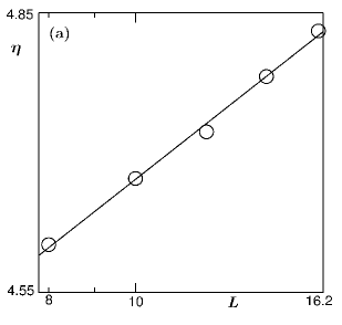
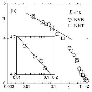
Figure 6: (a) Finite-size scaling estimation of critical exponent $x_{\eta}$. Here we have plotted $\eta$ as a function of $L$. For each value of $L$, calculation was done at the corresponding $T_{c}^{L}$. A double-log scale is used. The continuous line there has the theoretical exponent $0.068$. (b) The NHT and NVE data from Fig. 3 are plotted vs $\epsilon$, on double-log scale. The inset contains data for only the four smallest values of $\epsilon$, from NVE calculations. The solid lines in (b) correspond to the theoretical expectation.

In Fig. 5, we show $\eta(t)$ as a function of $t$, at $T_{c}^{L}$ of three different system sizes. The estimates of $\eta$ from the flat regions of these plots are demonstrated. These values are plotted in Fig. 6(a), as a function of $L$. On the log-log scales, the data appear fairly linear, indicating a power-law behavior. The continuous line there is a fit to the form (16), providing $x_{\eta}\simeq 0.070$. This is in excellent agreement with the value $x_{\eta}\simeq 0.068$, predicted ferrell ; jkbphysa ; hao by the theory of Ferrell and Bhattacharjee. For more reliability of a number from fitting, one, of course, needs data for more number of $L$ values. But due to lack of self averaging, computations of collective properties from MD simulations are extremely difficult task.

Having confirmed the theoretical exponent, we move to check for the extent of critical region. In Fig. 6(b), we plot $\eta$, from both NVE and NHT calculations, as a function of $\epsilon$, for $L=10$, on log-log scales. It appears that data only upto 10% above $T_{c}$ are consistent with the theoretical exponent, represented by the solid line. This, of course, is in agreement with the experimental observations for both statics and dynamics. For statics, of course, computer simulation results also show enhancements only upto 10% away from the critical temperature. Interestingly, this is at deviation with the critical range of bulk viscosity and Onsager coefficient for this particular model das2006 ; dasjcp2006 ; roy1 ; roy2 . For these quantities, the expected power laws were observed upto even 100% above $T_{c}$. In the inset of Fig. 6(b) we show data only for four smallest values of $\epsilon$, from NVE calculation, which show reasonably good consistency with the (solid) theoretical line having exponent $x_{\eta}\nu=0.043$. A power law fit to this data set provides $0.039$, i.e., $x_{\eta}\simeq 0.062$. This smaller value can well be due to finite-size effects or statistical fluctuation. Note that the averaging statistics for these results were poorer than that in Fig. 6(a). In all these analysis, a background $\eta_{b}$ was not considered. Here note that, $\eta$ is expected to exhibit a multiplicative critical anomaly, i.e., the enhancement of $\eta$ should be proportional to $\eta_{b}$ newrev ; dsf2007 . The current set of simulation results, however, are inadequate to resolve this important issue which we leave out for future work. The range of observation of critical enhancement, discussed above, in fact, depends upon whether one looks at $\eta$ or $\eta/\eta_{b}$. The lack of knowledge about $\eta_{b}$ prevents us from the latter exercise.

IV Conclusion

In summary, we have studied the critical behavior of shear viscosity in a symmetrical binary Lennard-Jones fluid. Canonical ensemble calculations with Nosé-Hoover thermostat (NHT) provide shear viscosity comparable to the ones computed from microcanonical ensemble. Better momentum conserving thermostats are, of course, available schmid . But appropriate compromise between momentum conservation and temperature control is essential.

Finite-size scaling analysis of our NHT simulation data show nice agreement with theoretical expectation. This is the first simulation confirmation of the critical anomaly of shear viscosity, irrespective of a liquid-liquid or vapor-liquid transition. Before this, to the best of our knowledge there were three simulation studies yeth2 ; dasjcp2006 ; roy2 on dynamic critical phenomena, where results for shear viscosity were also presented. In one of these studies dasjcp2006 , accepting the theoretical exponent, only the critical amplitude was estimated which had its relevance in obtaining a theoretical number for the critical amplitude of Onsager coefficient. In another study yeth2 , a statement about the upper bound of $x_{\eta}$ was made by using only two data points. These again are supportive of the difficulty one encounters in computational studies of such collective properties.

Our conclusions apply to the asymptotic critical behavior of a liquid mixture newrev . Here note that the asymptotic range for viscosity for vapor-liquid transition is limited to an extremely small range in the critical point vicinity and non-asymptotic corrections become essential for the understanding of experimental results mold1999 . This is related to the fact, as mentioned above, that the critical behavior of $\eta$ is proportional to $\eta_{b}$ which is much larger in a liquid mixture than in a vapor-liquid transition.

References

- (1) A. Onuki, Phase Transition Dynamics (Cambridge University Press, UK, 2002).
- (2) A. J. Bray, Adv. Phys. 51, 481 (2002).
- (3) J.-P. Hansen and I.R. Mcdonald, Theory of Simple Liquids (Academic Press, London, 2008).
- (4) M.P. Allen and D.J. Tildsely, Computer Simulations of Liquids (Clarendon, Oxford, 1987).
- (5) K. Jagannathan and A. Yethiraj, Phys. Rev. Lett. 93, 015701 (2004).
- (6) K. Jagannathan and A. Yethiraj, J. Chem. Phys. 122, 244506 (2005).
- (7) A. Chen, E.H. Chimowitz, S. De and Y. Shapir, Phys. Rev. Lett. 95, 255701 (2005).
- (8) S.K. Das, M.E. Fisher, J.V. Sengers, J. Horbach, and K. Binder, Phys. Rev. Lett. 97, 025702 (2006).
- (9) S.K. Das, J. Horbach, K. Binder, M.E. Fischer and J.V. Sengers, J. Chem. Phys. 125, 024506 (2006).
- (10) S. Roy and S.K. Das, Europhys. Lett. 94, 36001 (2011).
- (11) S. Roy and S.K. Das, J. Chem. Phys., 139, 064505 (2013).
- (12) J. Zinn-Justin, Phys. Repts. 344, 159 (2001).
- (13) J.V. Sengers and R.A. Perkins, Fluids near Critical Points, in Transport Properties of Fluids: Advances in Transport Properties, eds. M.J. Assael, A.R.H. Goodwin, V. Vesovic and W.A. Wakeham (IUPAC, RSC Publishing, Cambridge, 2014), pp. 337-361.
- (14) P.C. Hohenberg and B.I. Halperin, Rev. Mod. Phys. 49, 435 (1977).
- (15) L.P. Kadanoff and J. Swift, Phys. Rev. 166, 89 (1968).
- (16) M.A. Anisimov and J.V. Sengers, in Equations of State for Fluids and Fluid Mixtures, ed. J.V. Sengers, R.F. Kayser, C.J. Peters and H.J. White, Jr. (Elsevier, Amsterdam, 2000) p.381.
- (17) A. Onuki, Phys. Rev. E 55, 403 (1997).
- (18) G.A. Olchowy and J.V. Sengers, Phys. Rev. Lett. 61, 15 (1988).
- (19) R. Folk and G. Moser, Phys. Rev. Lett. 75, 2706 (1995).
- (20) H. Hao, R.A. Ferrell and J.K. Bhattacharjee, Phys. Rev. E. 71, 021201 (2005).
- (21) J.K. Bhattacharjee, I. Iwanowski and U. Kaatze, J. Chem. Phys. 131, 174502 (2009).
- (22) J.K. Bhattacharjee, U. Kaatze and S.Z. Mirzaev, Rep. Progr. Phys. 73, 066601 (2010).
- (23) J.V. Sengers and J.G. Shanks, J.Stat. Phys. 137, 857 (2009).
- (24) H.C. Burstyn and J.V. Sengers, Phys. Rev. Lett. 45, 259 (1980).
- (25) H.C. Burstyn and J.V. Sengers, Phys. Rev. A 25, 448 (1982).
- (26) D.P. Landau and K. Binder, A Guide to Monte Carlo Simulations in Statistical Physics, 3rd Edition (Cambridge University Press, Cambridge, 2009).
- (27) D. Frenkel and B. Smit, Understanding Molecular Simulations: From Algorithm to Applications (Academic Press, San Diego, 2002).
- (28) D.C. Rapaport, The Art of Molecular Dynamics Simulations (Cambridge University Press, Cambridge, UK, 2004).
- (29) S.D. Stayonav and R.D. Groot, J. Chem. Phys. 122, 114112.
- (30) P. Nikunen, M. Karttunen and I. Vattulainen, Comp. Phys. Comm. 153, 407 (2003).
- (31) M. Ripoll, M. Mussawisade, R. G. Winkler and G. Gompper, Phys. Rev. E 72, 016701 (2005).
- (32) M.E. Fisher, in Critical Phenomena, edited by M.S. Green (Academic Press, London, 1971) p.1.
- (33) R.A. Ferrell and J.K. Bhattacharjee, Phys. Rev. Lett. 88, 77 (1982).
- (34) J.K. Bhattacharjee and R.A. Ferrell, Physica A 250, 83 (1998).
- (35) M.P. Allen and F. Schmid, Molecular Simulation 33, 21 (2006).
- (36) S.K. Das, J.V. Sengers and M.E. Fisher, J. Chem. Phys. 127, 144506 (2007).
- (37) R.F. Berg, M.R. Moldover and G.A. Zimmerli, Phys. Rev. Lett. 82, 920 (1999).