Maximizing algebraic connectivity for certain families of graphs

Abstract

We investigate the bounds on algebraic connectivity of graphs subject to constraints on the number of edges, vertices, and topology. We show that the algebraic connectivity for any tree on $n$ vertices and with maximum degree $d$ is bounded above by $2\left(d-2\right)\frac{1}{n}+O\left(\frac{\ln n}{n^{2}}\right).$ We then investigate upper bounds on algebraic connectivity for cubic graphs. We show that algebraic connectivity of a cubic graph of girth $g$ is bounded above by $3-2^{3/2}\cos\left(\pi/\left\lfloor g/2\right\rfloor\right),$ which is an improvement over the bound found by Nilli [A. Nilli, Electron. J. Combin., 11(9), 2004]. Finally, we propose several conjectures and open questions.

AMS Subject Classification: 05C50, 68M10, 05C80.

Keywords: algebraic connectivity, optimal networks, trees, cubic graphs.

1 Introduction

This paper is motivated by the following question: among all possible networks connecting $n$ nodes, and subject to a specified resource or topology constraints, which one is the most effective at diffusing the flow of information? We are interested in the case where the network is undirected and all non-zero edges have the same weight.

One of the simplest ways of modelling the information flow in a network is the linear consensus model, which is widely used in control theory [1]:

$$\frac{du_{j}}{dt}=\sum_{j\neq i}e_{ij}\left(u_{i}-u_{j}\right).$$ (1)

Here $e_{ij}$ denote edge weights between nodes $i,j$ and $u_{j}$ is the “load” at node $j$; the information flows from $i$ to $j$ in proportion to the load differential between the nodes; $e_{ij}=1$ if $i$ and $j$ are joined by an edge and is zero otherwise. For large $t$ the solution to (1) is given by $u(t)\sim\bar{u}+Ce^{-\lambda_{2}t},$ where $\bar{u}$ is consensus (average) state and $\lambda_{2}$ is the second smallest eigenvalue of the graph Laplacian matrix $L=D-A$ where $A$ is the adjacency matrix and $D$ is the degree matrix (the smallest eigenvalue of $L$ is zero and $\lambda_{2}>0$ if and only if the network is connected). The eigenvalue $\lambda_{2}$ is often called the algebraic connectivity of the graph [2], and roughly, the larger $\lambda_{2},$ the faster $u$ diffuses to its consensus state. In this sense, the “optimal” network is the one which maximizes the algebraic connectivity, subject to given constraints. This leads to the following question.

Question: Which graphs maximize the algebraic connectivity, given a set of constraints on the number of vertices, edges, maximum degree, and graph topology?

This and related questions arise in many diverse areas, including optimal network topologies [3]; scheduling and network coding [4]; experimental design [5, 6], diffusion in small world networks [7, 8], synchronization in complex networks [9], and ranking algorithms [10, 11]. There is also a close link to expander graphs and Ramanujan graphs. These are graphs with “high” algebraic connectivity in some sense. See recent reviews [12, 13] and references therein. A nice recent survey on algebraic connectivity is [14].

In general, the problem of finding the optimal graph given $m$ edges and $n$ vertices is known to be NP-complete [15]. Despite this fact, several simple heuristics exist that can be used to obtain a graph with reasonably large algebraic connectivity [16, 17]. See also [18] for some results for almost-complete graphs, where $m$ is close to $n\left(n-1\right)/2.$ In [19, 20], the question of optimizing algebraic connectivity with respect to graph diameter was studied.

In this paper we are concerned with the regime where the number of edges $m$ grows in proportion to the number of vertices $n,$ so that the graph is relatively sparse. In particular, a random Erdos-Renyei graph with $O(n)$ edges is well known to be disconnected with high probability as $n\rightarrow\infty,$ so for such a graph, $\lambda_{2}=0$ almost surely [21, 22], and as such, random graphs are not good optimizers in this regime. The smallest value for $m$ for which the graph is connected is $m=n-1,$ in which case any connected graph is a tree (for disconnected graphs, $\lambda_{2}=0$ so we only consider connected case). Without a degree restriction, the star, which is a tree having a single root and $n-1$ leafs (see Figure 1(a)), is the unique optimizer of algebraic connectivity among all trees of $n$ vertices, with $\lambda_{2}=1$ when $n\geq 3$ [23, 14]. However, many trees of importance to applications have a degree restriction. For example, decision or binary trees have degree at most 3. Another important example are trees representing neuronal dendrites [24], which consist of mostly degree two vertices with an occasional degree 3 vertex (see [24] for further details). This motivates the following question.

Open question 1.1

Among all trees with $n$ vertices with maximal vertex degree $d,$ which tree maximizes the algebraic connectivity?

In this paper we give the following partial answer to this question:

Theorem 1.2

Let $T$ be any tree with $n$ vertices and maximum degree $d.$ Then $\lambda_{2}\left(T\right)\leq 2\left(d-2\right)\frac{1}{n}+O\left(\frac{\ln n}{n^{2}}\right)$ as $n\rightarrow\infty$ for fixed $d.$

A bound without the $O$ notation (valid even when $n=O(1)$), is given in (9).

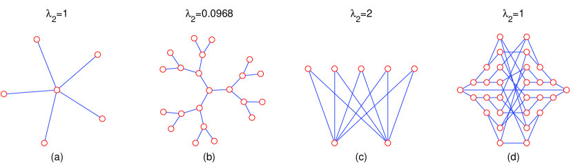
Figure 1: (a) The star, which is the maximizer of algebraic connectivity for all trees. (b) Maximally-balanced tree of degree at most $d$ with $n=\frac{d(d-1)^{K}-2}{d-2}$ vertices (here, $n=22,d=3,K=3$). (c) The complete bipartite graph $K_{2,n-2}$, which is a conjectured maximizer for all graphs of $n$ vertices with $m=2(n-2)$ edges. (d) The Tutte 8-cage, which is the conjectured maximizer for the cubic graphs with 30 vertices.

A well-known “basic” upper bound for algebraic connectivity for any tree is $\lambda_{2}(T)\leq 2-2\cos(\frac{\pi}{D+1}),$ where $D$ is the diameter of $T$ [14], and can be obtained by “pruning” any branches that are not along the longest path of the tree. This bound is attained for both the star graph and the path graph. However, in general, it is far from optimal when there is a restriction on the maximal degree of a tree. Among trees of maximal degree $d,$ one has $n\leq\frac{d\left(d-1\right)^{D/2}-2}{d-2}$ (the equality is achieved only for a maximally balanced tree such as shown in Figure 1(b). A maximally balanced tree is a tree whose leafs are all at the same distance from a root vertex and whose non-leaf vertices all have the same degree). For fixed $d$ and large $n,$ this yields $D\geq O(\ln n)$ so that the “basic” bound is $\lambda_{2}(T)\leq O(1/\ln^{2}(n)),$ which is much worse than the $O(1/n)$ bound of Theorem 1.2. The lower bound for the algebraic connectivity of any tree of $n$ vertices is attained by the path graph for which $\lambda_{2}=2-2\cos(\frac{\pi}{n})=O(\frac{1}{n^{2}})$, so that in general, $O(1/n^{2})\leq\lambda_{2}\leq O(1/n)$.

The algebraic connectivity of a maximally balanced tree such as shown in Figure 1(b) can be determined explicitly, as was done for example in [25, 26, 27]. It was found that $\lambda_{2}\sim\frac{d}{d-1}\left(d-2\right)\frac{1}{n}$ as $n\rightarrow\infty$ for such a tree. So the bound in Theorem 1.2 is not optimal; in fact we conjecture that $\frac{d}{d-1}\left(d-2\right)\frac{1}{n}$ is the asymptotically optimal upper bound as $n\to\infty$. See Section 4 for further discussion and a related conjecture.

In Section 3 we explore optimal cubic (i.e. 3-regular) graphs, which have $m=3n/2$ edges. We are motivated by the following question.

Open question 1.3

Among all cubic (i.e. 3-regular) graphs with $n$ vertices, which one maximizes the algebraic connectivity?

Regular graphs appear in numerous applications where having high connectivity is important. It is well known that the expected algebraic connectivity of a random cubic graph is $\lambda_{2}\sim 3-2\sqrt{2}+O(1/\ln(n))$ as $n\rightarrow\infty$ (see [28, 29, 30, 31]). So unlike the case of trees of maximum degree 3, the maximum possible connectivity of a cubic graph is bounded away from zero. One of the applications of this fact is that a random cubic graph is an expander graph with very high probability [32, 33].

The best known bound for $\lambda_{2}$ was obtained by Nilli in [34]. He showed that for any cubic graph, $\lambda_{2}\leq 3-2\sqrt{2}\cos\left(2\pi/D\right)$ where $D$ is its diameter. However so far, there is no example of a cubic graph that we know of, which actually attains this bound. In Section 4 we suggest a possible optimal bound when $n=2^{K}-2,$ which is tighter than Nilli’s bound, and which is achieved at least for $n=6,14,30$ and $126$. This is discussed in Conjecture 4.5. Related to this conjecture, we prove the following result.

Theorem 1.4

Suppose that a cubic graph $G$ of $n$ edges has girth $g$. Then $\lambda_{2}\left(G\right)\leq 3-2\sqrt{2}\cos\left(\pi/\left\lfloor g/2\right\rfloor\right).$

For some graphs, this bound is actually achieved; see Figure 1(d) and Section 4. As shown in Remark 3.2 below, the bound of Theorem 1.4 is better the result obtained by Nilli in [34], which is $\lambda_{2}\left(G\right)\leq 3-2\sqrt{2}\cos\left(2\pi/\left\lfloor g/2\right\rfloor\right).$

Finally, in Section 4, we discuss some numerical results, open questions and several conjectures, including the following conjecture:

Conjecture 1.5

Among all graphs with exactly $n$ vertices and $m=2\left(n-2\right)$ edges, a graph which maximizes the algebraic connectivity is the complete bipartite graph $K_{2,n-2}$ (see Figure 1(c)), with $\lambda_{2}(K_{2,n-2})=2.$

2 Trees

In this Section we prove Theorem 1.2. We recall the alternative definition of $\lambda_{2}$ for a graph $G$ on $n$ vertices using the Rayleigh quotient [14],

$$\lambda_{2}=\min_{\begin{subarray}{c}x\in\mathbb{R}^{n}\text{ subject to}\\ x_{1}+\cdots+x_{n}=0\end{subarray}}\frac{\sum_{(i,j)\in E(G)}\left(x_{i}-x_{j}\right)^{2}}{\sum_{j=1}^{n}x_{j}^{2}}.$$ (2)

We first need the following concept of a “modified” Laplacian eigenvalue. Given a graph $G$ and a vertex $r\in V(G),$ define

$$\tilde{\lambda}(G,r):=\min_{x\in\mathbb{R}^{n}}\frac{x_{r}^{2}+\sum_{\left(i,j\right)\in E(G)}\left(x_{j}-x_{i}\right)^{2}}{\sum_{j=1}^{n}x_{j}^{2}}$$ (3)

An alternative definition is that $\tilde{\lambda}$ is the smallest eigenvalue of the eigenvalue problem

$$\left\{\begin{array}[c]{c}\tilde{\lambda}x_{j}=\sum_{\left(i,j\right)\in E(G)}\left(x_{j}-x_{i}\right),\ \ \text{if }j\neq r\\ \tilde{\lambda}x_{j}=x_{j}+\sum_{\left(i,j\right)\in E(G)}\left(x_{j}-x_{i}\right),\ \text{if}\ j=r\end{array}\right.$$ (4)

The proof of Theorem 1.2 relies on the following three lemmas:

Lemma 2.1

Let $T$ be a tree with $n$ vertices each of degree at most $d,$ and whose root $r$ has degree at most $d-1$. Then $\tilde{\lambda}(T,r)\leq\frac{d-2}{d-1}\frac{1}{n}+O\left(\frac{\ln n}{n^{2}}\right).$

Lemma 2.2

Given a graph $G,$ and a vertex $v$ with at least two edges $\left(v,u\right)$ and $\left(v,w\right)$ such that removing $v$ separates $G$ into at least two or more disjoint subgraphs $G_{1},G_{2}\ldots,$ such that $u\in V(G_{1})$ and $w\in V(G_{2}).$ Then

$$\lambda_{2}(T)\leq\max\left(\tilde{\lambda}\left(G_{1},u\right),\tilde{\lambda}\left(G_{2},w\right)\right).$$

Lemma 2.3

Let $T$ be a tree with $n$ vertices and of maximal degree $d.$ Then there exists a vertex $v\in V(T)$ such that removing $v$ and its associated edges separates $T$ into subtrees such that at least two of these subtrees have at least $\frac{n-2}{2(d-1)}$ vertices.

Proof of Lemma 2.1. Choose unique positive integers $m$ and $K$ such that

$$n =1+(d-1)+(d-1)^{2}+\cdots+(d-1)^{K-1}+m,\ \ \ \ \text{with }0\leq m<(d-1)^{K}$$

$$=\frac{(d-1)^{K}-1}{d-2}+m.$$ (5)

Sort the vertices according to their distance from the root, from smallest to largest. After sorting them, let $V_{1}$ be the set containing the first vertex in the list, i.e. root vertex; let $V_{2}$ contain the next $d-1$ vertices; let $V_{3}$ contain the next $(d-1)^{2}$ vertices and so on up to $V_{K}$ which contains $\left(d-1\right)^{K-1}$ vertices, and with $V_{K+1}$ containing the remaining $m$ vertices. For vertex $j\in V_{k}$, assign a weight $x_{j}=1-\left(\frac{1}{d-1}\right)^{k}.$

For a non-root vertex $j\in V(T),j\neq r,$ let $parent(j)\in V(T)$ denote its parent, that is the neighbouring vertex that is closer to the root $r$. We then have

$$x_{r}^{2}+\sum_{\left(i,j\right)\in E(T)}\left(x_{j}-x_{i}\right)^{2} =x_{r}^{2}+\sum_{j\in V(T),\ j\neq r}\left(x_{j}-x_{parent(j)}\right)^{2}$$

$$=x_{r}^{2}+\sum_{k=2}^{K+1}\sum_{j\in V_{k}}\left(x_{j}-x_{parent(j)}\right)^{2}$$

Moreover, if $j\in V_{k}$ with $k>1,$ then either $parent(j)\in V_{k}$ or else $parent(j)\in V_{k-1}.$ In both cases, we have

$$\left(x_{j}-x_{parent(j)}\right)^{2}\leq\left(\frac{1}{(d-1)^{k}}-\frac{1}{\left(d-1\right)^{k-1}}\right)^{2}=\frac{\left(d-2\right)^{2}}{\left(d-1\right)^{2k}}$$

so that

$$x_{r}^{2}+\sum_{\left(i,j\right)\in E(T)}\left(x_{j}-x_{i}\right)^{2} \leq\left(\frac{d-2}{d-1}\right)^{2}+\sum_{k=2}^{K}(d-1)^{k-1}\frac{\left(d-2\right)^{2}}{\left(d-1\right)^{2k}}+m\frac{\left(d-2\right)^{2}}{\left(d-1\right)^{2\left(k+1\right)}}$$ (6)

$$=\frac{d-2}{d-1}-\frac{d-2}{(d-1)^{K}}+m\frac{\left(d-2\right)^{2}}{\left(d-1\right)^{2\left(k+1\right)}}$$

$$\sim\frac{d-2}{d-1}+O(1/n).$$

Similarly, we write

$$\sum_{i\in V(T)}x_{i}^{2}=\sum_{k=2}^{K}\sum_{j\in V_{k}}x_{j}^{2}.$$

Moreover, for $j\in V_{k},$ we have $x_{j}=1-\left(\frac{1}{d}\right)^{k}$ so that

$$\sum_{i\in V(T)}x_{i}^{2} =\sum_{k=2}^{K}(d-1)^{k-1}\left(1-\left(\frac{1}{d-1}\right)^{k}\right)^{2}+m\left(1-\left(\frac{1}{d-1}\right)^{K+1}\right)^{2}$$ (7)

$$=\left(\frac{\left(d-1\right)^{K}}{\left(d-2\right)}+m\right)\left[1+O\left(\frac{K}{\left(d-1\right)^{K}}\right)\right]$$

$$=n\left(1+O(K/n)\right)$$

Therefore

$$\frac{x_{r}^{2}+\sum_{\left(i,j\right)\in E(T)}\left(x_{j}-x_{i}\right)^{2}}{\sum_{j=1}^{N}x_{j}^{2}}=\frac{d-2}{d-1}\frac{1}{n}+O(K/n^{2}).$$

Moreover, note from definition (5) of $m$ and $K$ that $K=O(\ln n)$ so that $O(K/n^{2})=O(\left(\ln n\right)/n^{2}).$ Recalling the definition (3) of $\tilde{\lambda}$ completes the proof of the lemma. $\blacksquare$

Remark 2.4

The $O$ notation can be avoided by computing all the terms in (6) and (7). Setting $m=0,$ we then obtain the upper bound without the $O$ notation,

$$\tilde{\lambda}\leq\frac{\left(d-2\right)^{2}}{(d-1)^{K+1}}\left(\frac{1-\frac{1}{(d-1)^{K-1}}}{1-\frac{2(K-1)}{\left(d-1\right)^{K}}(d-2)-\frac{d-1-\left(d-1\right)^{-2}}{\left(d-1\right)^{K}}-\frac{1}{\left(d-1\right)^{2K+1}}}\right).$$ (8)

The same bound is valid even if $m>0$, because appending leafs to a tree only decreases $\tilde{\lambda}$ (see [14]). The bound (8) is very close (but not identical) to the upper bound as was obtained for Bethe trees with $k=K+1$ levels in [25, 27] using a related method.

Proof of Lemma 2.2. Let $x$ be the eigenvector corresponding to $\tilde{\lambda}(G_{1},u)$ and $y$ be the eigenvector corresponding to $\tilde{\lambda}(G_{2},w),$ so that $x_{j}=0$ for all $j\notin V(G_{1})$ and similarly $y_{j}=0$ for all $j\notin V(G_{2}).$

Consider any linear combination $z=\alpha x+\beta y.$ Note that $z_{v}=0$ and we have

$$\sum_{(i,j)\in E(G)}\left(z_{i}-z_{j}\right)^{2}=\alpha^{2}\left(\sum_{(i,j)\in E(G_{1})}\left(x_{i}-x_{j}\right)^{2}+x_{u}^{2}\right)+\beta^{2}\left(\sum_{(i,j)\in E(G_{2})}\left(y_{i}-y_{j}\right)^{2}+y_{w}^{2}\right).$$

Moreover by orthogonality, we have $\left|z\right|^{2}=\alpha^{2}\left|x\right|^{2}+\beta^{2}\left|y\right|^{2}.$ Define

$$R_{1}(x):=\dfrac{\sum_{(i,j)\in E(G_{1})}\left(x_{i}-x_{j}\right)^{2}+x_{u}^{2}}{\sum_{i\in V(G_{1})}x_{i}^{2}},\ \ \ \ \ R_{1}(y):=\dfrac{\sum_{(i,j)\in E(G_{2})}\left(y_{i}-y_{j}\right)^{2}+y_{w}^{2}}{\sum_{i\in V(G_{2})}y_{i}^{2}}$$

so that $\tilde{\lambda}(G_{1},u)=R_{1}(x),\$ $\tilde{\lambda}(G_{2},w)=R_{2}(y).$ We have

$$\frac{\sum_{(i,j)\in E(G)}\left(z_{i}-z_{j}\right)^{2}}{\left|z\right|^{2}} =\dfrac{\alpha\left(\sum_{(i,j)\in E(G_{1})}\left(x_{i}-x_{j}\right)^{2}+x_{u}^{2}\right)+\beta\left(\sum_{(i,j)\in E(G_{2})}\left(y_{i}-y_{j}\right)^{2}+y_{w}^{2}\right)}{\alpha^{2}\left|x\right|^{2}+\beta^{2}\left|y\right|^{2}}$$

$$=R_{1}(x)\frac{\alpha^{2}\left|x\right|^{2}}{\alpha^{2}\left|x\right|^{2}+\beta^{2}\left|y\right|^{2}}+R_{2}(y)\frac{\beta^{2}\left|y\right|^{2}}{\alpha^{2}\left|x\right|^{2}+\beta^{2}\left|y\right|^{2}}$$

$$\leq\max(R_{1}(x),R_{2}(y))$$

$$\leq\max\left(\tilde{\lambda}(G_{1},u),\tilde{\lambda}(G_{2},w)\right).$$

Now choose $\alpha,\beta$ such that $\sum_{i\in V(G)}z_{i}=0$. That is, take $\frac{\alpha}{\beta}=-\left(\sum_{i\in V(G_{2})}y_{i}\right)/\left(\sum_{i\in V(G_{1})}x_{i}\right)$ as long as $\sum_{i\in V(G_{1})}x_{i}\neq 0;$ in the contrary case take $\alpha=1,\beta=0.$ Then from the definition (2) of $\lambda_{2},$ we get

$$\lambda_{2}\leq\frac{\sum_{(i,j)\in E(G)}\left(z_{i}-z_{j}\right)^{2}}{\left|z\right|^{2}}\leq\max\left(\tilde{\lambda}(G_{1},u),\tilde{\lambda}(G_{2},w)\right)$$

which concludes the proof. $\blacksquare$

We note that an alternative proof of Lemma 2.2 can be given using the mini-max definition of $\lambda_{2}$, as done by Nilli in [34].

Proof of Lemma 2.3. The algorithm to find $v$ is simple: start with an arbitrary vertex $v_{0}$ in $T.$ Choose a neighbour $v_{1}$ of $v_{0}$ which belongs to the subtree with the largest number of vertices, among all the subtrees that are obtained by deleting $v_{0}$ from $T$ (in case of a tie, choose a vertex deterministically, e.g. the one with the smallest index). Continue this process, obtaining a sequence of vertices $v_{0},v_{1},v_{2},\ldots$ This sequence eventually settles to a two-cycle $v,w,v,w,\ldots$ When this happens, consider the two subtrees obtained by deleting the edge $(v,w),$ call them $T_{1}$ and $T_{2}.$ One of these tree, say tree $T_{1}$ containing $v,$ has at least $n/2$ vertices. Upon deleting $v$ from this tree, we get at most $d-1$ subtrees of $T_{1}$. So one of these subtrees must have the size at least ($n/2-1)/(d-1)=\frac{n-2}{2(d-1)}$ vertices. But then the second tree $T_{2}$ containing $w$ must have at least $\frac{n-2}{2(d-1)}$ vertices also, since it is the subtree that contains the most vertices among all subtrees obtained by deleting $v.$ So $v$ is the desired vertex. $\blacksquare$

We are now in position to prove the main theorem of this paper.

Proof of Theorem 1.2. Choose a vertex $v$ using Lemma 2.3, which separates the tree into at least two subtrees whose sizes are $n_{1},n_{2}\geq\frac{n-2}{2(d-1)}.$ Applying Lemmas 2.2 and 2.1 to these subtrees we obtain

$$\lambda_{2}(T)\leq\frac{d-2}{d-1}\max\left(\frac{1}{n_{1}},\frac{1}{n_{2}}\right)+O\left(\frac{\ln n}{n^{2}}\right)\leq\frac{d-2}{d}\frac{2}{n}+O\left(\frac{\ln n}{n^{2}}\right).\ \ \ \ \ \ \ \ \ \ \ \blacksquare$$

The bound in Theorem 1.2 can be written without the $O$ notation, by replacing the estimate for $\tilde{\lambda}$ in Lemma 2.1 with the estimate (8). To do this, choose $K$ in (8) in such a way that the number of vertices in two subtrees produced by Lemma 2.3 is more than $\frac{\left(d-1\right)^{K}-1}{d-2}$ (formula (5) with $m=0).$ That is, choose $K$ such that $\frac{\left(d-1\right)^{K}-1}{d-2}\leq\frac{n-2}{2(d-1)}.$ We then obtain an upper bound without the $O$ notation, namely that

$$\lambda_{2}\leq\text{right hand side of (\ref{precise2}) with }K=\left\lfloor\log_{d-1}\left(1+\frac{\left(d-2\right)\left(n-2\right)}{2\left(d-1\right)}\right)\right\rfloor.$$ (9)

3 Cubic graphs

In this Section we give the proof of Theorem 1.4. It is a direct consequence of the following lemma.

Lemma 3.1

Let $T_{K}$ be a graph consisting of two perfect binary trees of height $K$ joined by an edge connecting their roots as illustrated here (with $K=3$):

$$K=3$$

Suppose that a cubic graph $G$ has $T_{K}$ as its subgraph. Then $\lambda_{2}(G)\leq 3-2^{3/2}\cos(\pi/K)$.

Above, we defined the height $K$ of a perfect binary tree as one less than the distance from any leaf to its root.

Remark 3.2

It was shown by Nilli [34] that for any cubic graph $G,$ $\lambda_{2}(G)\leq 3-2^{3/2}\cos\left(2\pi/D\right)$ where $D$ is the diameter of the graph. If $G$ has $T_{K}$ as its subgraph, then it has two vertices that are separated by distance at least $K$: take the first vertex to be the root of one of the two binary trees that make up $T_{K}$ and take the second vertex to be one of the leafs of the other subtree. So Nilli’s bound for the algebraic connectivity of $G$ is $3-2^{3/2}\cos(2\pi/K)$. Thus, Lemma 3.1 is an improvement over Nilli’s bound for the case where $T_{K}$ is a subgraph of $G.$ Similarly, a graph of girth $g$ has diameter at least $\left\lfloor g/2\right\rfloor,$ so that Nilli’s bound is $3-2^{3/2}\cos(2\pi/\left\lfloor g/2\right\rfloor)$ which is worse than the result of Theorem 1.4.

Proof. Consider the following choice of weights $x_{j},j\in V(G)$: for nodes at level $k$ on the right tree, assign weight $x_{j}=v_{k},$ where $v_{k}$ will be specified below; for nodes at level $k$ on the left tree, assign weight $x_{j}=-v_{k}$. For all other nodes, assign weight zero. With this choice, the sum of all the weights is zero, so that $\left(x_{1},\ldots,x_{n}\right)\perp\left(1,1,\ldots,1\right)$. Now consider any leaf vertex of $T_{K}.$ It has three edges: one that connects it to its parent, and two other edges that connect it to either another leaf whose weight is $\pm v_{K}$ or to a vertex outside $T_{K}$ whose weight is zero. Therefore if $\left(v,w\right)$ is an edge that connects $v$ to the non-parent vertex $w$ and $a,b$ are the weights of $v$ and $w$ respectively, then $\left(a-b\right)^{2}\leq\left(v_{K}-(-v_{K})\right)^{2}.$

It follows that $\lambda_{2}(G)$ bounded by any eigenvalue $\mu$ of the eigenvalue problem

$$\mu v_{1} =\left(v_{1}-(-v_{1})\right)+2\left(v_{1}-v_{2}\right);$$ (10)

$$\mu v_{j} =v_{j}-v_{j-1}+2\left(v_{j}-v_{j+1}\right),\ \ \ j=2\ldots K-1$$ (11)

$$\mu v_{K} =v_{K}-v_{K-1}+2(v_{K}-(-v_{K})),$$ (12)

corresponding to the $K$ by $K$ matrix

$$M=\left[\begin{array}[c]{cccccc}4&-2&&&&\\ -1&3&-2&&&\\ &-1&\ddots&\ddots&&\\ &&\ddots&3&-2&\\ &&&-1&3&-2\\ &&&&-1&5\end{array}\right]$$

Similar types of Toeplitz matrices are well-known and occur in many related problems, for example when computing eigenvalues of Bethe trees [25, 27]. For reader’s convenience, here we show directly that its eigenvalues are given by $\mu=3-2^{3/2}\cos(\pi k/K),$ $k=1\ldots K.$

We have the following self-consistent anzatz for the eigenvector:

$$v_{j}=Az^{j}+B\left(\frac{1}{2z}\right)^{j},$$ (13)

where $A,B$ and $z$ are to be found. Then it is easy to check that $\mu v_{j}=v_{j}-v_{j-1}+2\left(v_{j}-v_{j+1}\right)$ holds for any $j,A,B$ whenever

$$\mu=3-2z-\frac{1}{z}.$$ (14)

Write (10) as

$$\mu v_{1}=3v_{1}-2v_{2}-v_{0}+v_{0}+v_{1}.$$

It follows that $v_{0}+v_{1}=0$ so that $A=-B.$ Similarly, from the last row we obtain $2v_{k}+2v_{K+1}=0,$ which yields an equation for $z.$ After some algebra, this equation simplifies to

$$z^{-2K}=2^{K},\ \ z\neq\left(1/2\right)^{1/2}.$$

so that $z=\left(\frac{1}{2}\right)^{1/2}e^{\frac{2\pi ij}{2K}}.$ The choice $j=0$ corresponds to $v_{j}=0$ for all $j$ so this is not allowed. The remaining choices are

$$\mu=3-2\sqrt{2}\cos(\pi j/K),\ \ \ j=1\ldots K$$

The smallest eigenvalue among these corresponds to the choice $j=1,$ which is precisely the bound of the lemma. $\blacksquare$

Proof of Theorem 1.4. A cubic graph of girth $g$ has a subtree $T_{K}$ as defined in Lemma 3.1, where $K$ is any integer at most $g/2.$ Applying Lemma 3.1 completes the proof. $\blacksquare$

4 Computer experiments, open questions, discussion

We used the software Nauty [35] to generate all non-isomorphic trees of maximal degree $d=3$ up to $n=23$ vertices (according to Nauty, there are 565734 such trees with $n=23$). We then computed the tree which maximizes $\lambda_{2}.$ The result is shown in Figure 2. In all cases, the optimum tree was “well-balanced” in the sense that there was a central vertex whose removal subdivides the tree into three nearly equal subtrees. The maximizing tree was also unique. In the cases when $n=\frac{d\left(d-1\right)^{K}-2}{d-2}$ (see Figure 2, $n=10$ or $n=22$), the optimal tree appears to be the well-balanced Bethe tree whose algebraic connectivity is well-studied [25, 26, 27], and is asymptotic to $\lambda_{2}\sim\frac{d}{d-1}\left(d-2\right)\frac{1}{n}$. These computations suggest that the bound $\lambda_{2}\left(T\right)\leq 2\left(d-2\right)\frac{1}{n}+O\left(\frac{\ln n}{n^{2}}\right)$ of Theorem 1.2 is not optimal. We propose the following optimal bound:

Conjecture 4.1

Let $T$ be a tree with $n$ vertices and maximum degree $d.$ Then $\lambda_{2}\left(T\right)\leq\frac{d\left(d-2\right)}{d-1}\frac{1}{n}+O\left(\frac{\ln n}{n^{2}}\right)$ as $n\rightarrow\infty$ for fixed $d.$

In particular this conjecture is true for the well-balanced Bethe trees mentioned above. A stronger version of this conjecture is

Conjecture 4.2

Let $T$ be a tree with $n=\frac{d\left(d-1\right)^{K}-2}{d-2}$ vertices and maximum degree $d.$ Then its algebraic connectivity is less than the algebraic connectivity of the well-balanced Bethe tree with $n$ vertices whose non-leaf vertices have degree $d$.

We verified this conjecture using Nauty with $d=3$ and $n=10$ and $22$.

The bottleneck for improving Theorem 1.2 into Conjecture 4.1 is Lemma 2.3. It states, roughly, that there is a “central vortex” whose removal subdivides the tree into $d$ trees such that at least two have $\sim n/(2\left(d-1\right))$ vortices. Indeed Conjecture 4.1 is true for trees that are “well balanced” in the following sense:

Proposition 4.3

Suppose that a tree $T$ of order $n$ and maximal degree $d$ has a vertex whose removal subdivides $T$ into subtrees such that at least two of the subtrees have at least $\left(n-1\right)/d$ vertices. Then Conjecture 4.1 is true.

The proof of this proposition is identical to Theorem 1.2, except that the bound $\frac{n-2}{2(d-1)}$ in Lemma 2.3 gets replaced by $\frac{n-1}{d}$, and therefore the prefactor $2\left(d-2\right)$ in Theorem 1.2 gets replaced by $\frac{d\left(d-2\right)}{d-1}.$

Proposition 4.3 is applicable to all “maximal” trees in Figure 2 as they happen to be “well-balanced”. But most trees are not so well balanced. For example consider the following tree of 22 vertices:

Proposition 4.3 is not applicable to this tree: for example removing vertex 10 results in three subtrees of size 9, 6 and 6 whereas $(n-1)/d=7>6.$ Removing other vertices is even worse. Nonetheless for this tree, $\lambda_{2}=0.0835$ which is smaller than $\lambda_{2}=0.0936$ of the well-balanced tree of 22 vertices.

Consider again Conjecture 1.5, which states that $K_{2,n-2}$ has optimal algebraic connectivity $\lambda_{2}=2$ among all graphs with $m=2\left(n-2\right)$ edges. We used Nauty to exhaustively search through all graphs with $m=2\left(n-2\right)$ edges and with $n$ up to 13, and chose those with highest algebraic connectivity. The “winners” of this race are shown in Figure 3. For all $n$ we tested, the highest connectivity $\lambda_{2}=2$ was attained by the complete bipartite graph $K_{2,n-2},$ although depending on $n,$ several other graphs also had this connectivity. For example when $n=10,$ there are two graphs with $\lambda_{2}=2$: one is the Petersen graph and the other is the complete bipartite graph $K_{2,8}.$ The number of graphs with $m=2\left(n-2\right)$ edges seems to increase very fast with $n$: for example Nauty returned $\approx 2.7\times 10^{7}$ non-isomorphic connected graphs with $12$ vertices and $20$ edges whose minimum degree is 2, making it prohibitively expensive to do an exhaustive search for bigger values of $n$ (we restricted the minimum degree to 2 because $\lambda_{2}$ is bounded by $\frac{n}{n-1}d$ where $d$ is the minimum degree, and since we are only interested in $\lambda_{2}$ well above 1). For $n=13$ (and $m=22$) we only searched through graphs whose minimum degree is 3, of which there are were about $1.6\times 10^{6}$.

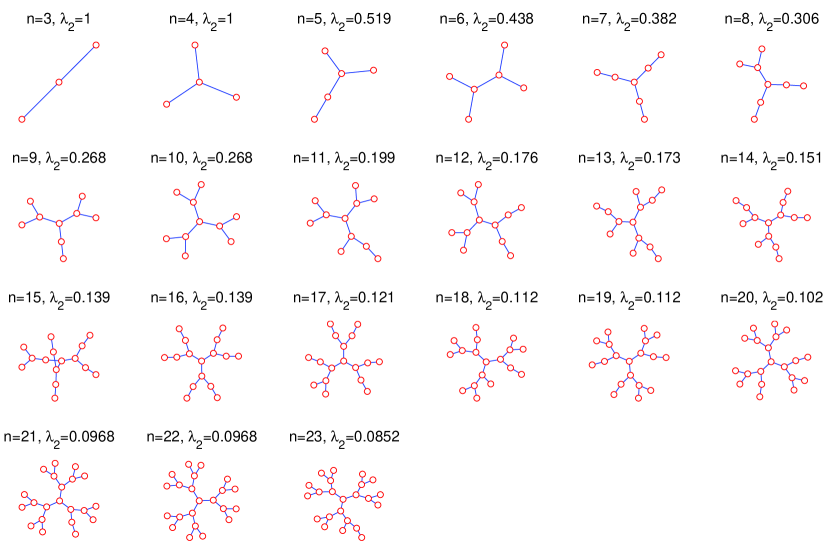
Figure 2: Trees of degree 3 on $n$ vertices that have maximum possible the algebraic connectivity for a given $n$.

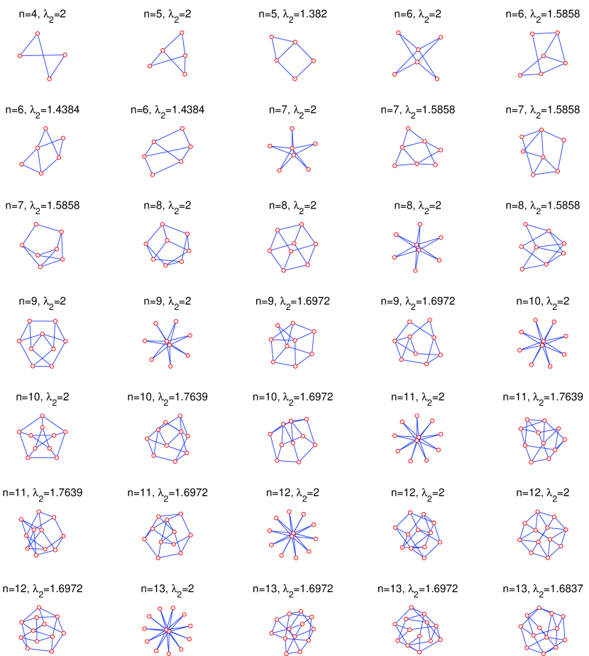
Figure 3: Graphs with maximal algebraic connectivity with $m=2(n-2)$ edges. Exhaustive search through all such graphs was done using Nauty program up to $n=12$. For $n=13$, it was confirmed $\lambda_{2}\leq 1.6972$ for graphs with minimum degree 3 (graphs with minimum degree 2 have $\lambda_{2}$ at most 2n/(n-1)).

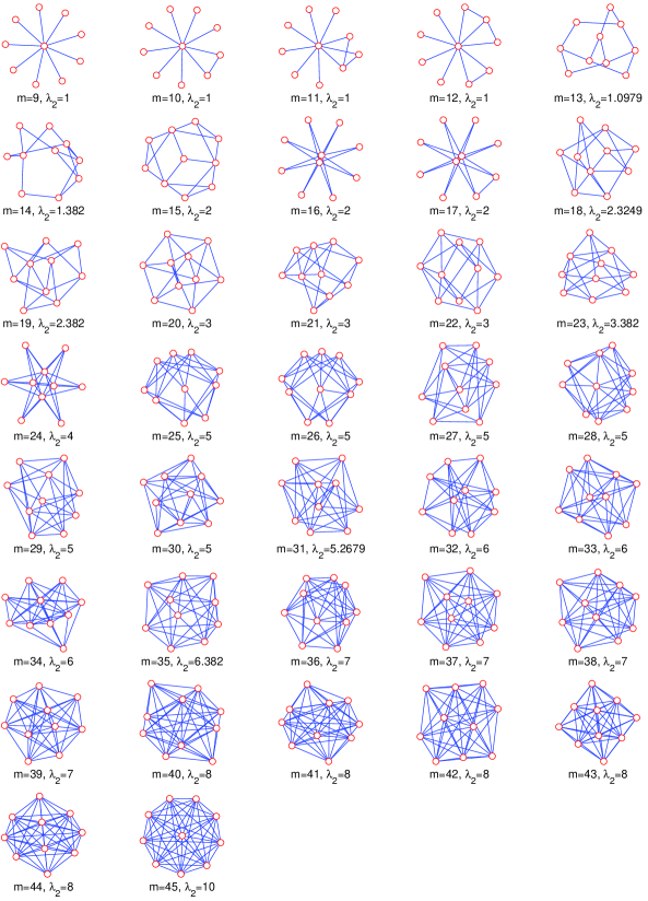
Figure 4: Some of the “winning” graphs that have maximum possible algebraic connectivity with $n=10$ vertices and $m$ edges, with $m$ as indicated. For some $m$, multiple maximizers exist but only one is shown.

For larger $n,$ there appears to be a large jump between the maximum value $\lambda_{2}=2$ and the next biggest value. For example with $n=13,$ the next maximal value is 1.6972, with nearly uniform degree distribution (all vertices have degree 3 or 4). The jump to the next $\lambda_{2}$ is much smaller (1.6837). As far as we can tell, with the exception of $K_{2,n-2},$ all other optimal or nearly-optimal graphs have vertices of degree either 3 or 4.

In Figure 4 we list maximal graphs with $n=10$ and with varying $m.$ Complete bipartite graphs with $m=b\left(n-b\right)$ are maximizers with $\lambda_{2}=b,$ when $b=2,3,4,5$ and $n=10.$ It may be tempting to generalize Conjecture 1.5 as follows:

Is it true that among graphs of $n$ vertices and $m=b\left(n-b\right)$ edges, the graph with the highest algebraic connectivity of $\lambda_{2}=b$ is attained by the complete bipartite graph $K_{b,n-b}$ when $b<n/2$?

In fact, the answer is false: it is known that for a random $d-$regular graph, the expected algebraic connectivity is $\lambda_{2}\sim d-2\sqrt{d-1}$ as $n\rightarrow\infty$ [28, 30, 31]. Such graph has $m=dn/2$ edges. For large $m,$ this corresponds to $b\sim d/2.$ Setting $d/2\sim$ $d-2\sqrt{d-1},$ we obtain that at least for $d\geq 15$ and large $n,$ a random $d$-regular graph has higher connectivity than $K_{b,n-b}$ with $b=d/2,$ with very high probability. In other words, if $b\geq 8,$ $K_{b,n-b}$ is not the maximizer of $\lambda_{2}$ among the graphs of $b\left(n-b\right)$ vertices. This leads to the following question:

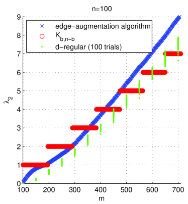
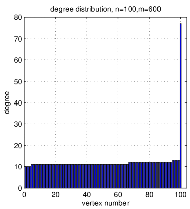
Figure 5: Left: Comparison of algebraic connectivity obtained from edge-augmentation algorithm versus $d$-regular graphs and bipartite complete graphs $K_{b,n-b}$. For a given number of edges $m$, $b$ is taken to be the largest integer such that $b(n-b)\leq m$ whereas $d=2m/n$. Right: The distribution of degrees as obtained by the edge-augmentation algorithm with $n=100,m=600$. In this regime the edge-augmentation beats the both the $d$-regular graph (with $d=12$) and $K_{b,n-b}$ (with $b=6$). Note the presence of a high-degree vertex.

Open question 4.4

Among graphs with $m=bn$ edges, what is the degree distribution for that maximizes the algebraic connectivity, when $b\geq 8,$ $b=O(1),$ and $n\rightarrow\infty?$

We speculate that this question could have implications for airline network design. Most major US airlines utilize “hub-network” with several large airports serving multiple smaller airports. This is similar to the complete bipartite graph $K_{b,n-b}.$ However the above results suggest that for airlines with more than 8 hubs, it is may be better to switch to more uniform topology, with each airport having roughly similar number of connections to others. Of course, there are many other factors to consider for airlines, such as city size and popular travel destinations, as well as the physical distance between cities. To what extent the algebraic connectivity plays any role in airport design is unclear.

For values of $n>12$, exhaustive search is impractical and heuristic algorithms to maximize connectivity need to be used. In [16],[17], the following “edge-augmentation” heuristic algorithm was suggested to find graphs with $n$ vertices and $m$ edges having relatively high algebraic connectivity:

1. Start with an empty graph of $n$ vertices.

2. Compute the eigenvector $v$ corresponding to $\lambda_{2}(G).$

3. Find vertices $i,j$ for which $\left|v_{i}-v_{j}\right|$ is is maximum. Add an edge $\left(i,j\right)$ to $G.$

4. Repeat steps 2 and 3 until the graph has $m$ edges.

The edge-augmentation gives better results when compared with $d$-regular graphs, for the same number of edges $m=dn/2$. However for $b<5$ and with $m=b(n-b)$, the complete bipartite graph $K_{b,n-b}$ has $\lambda_{2}=b$, which is better than the edge-augmentation. On the other hand, edge-augmentation overtakes both complete bipartite graph when $b>6,$ as well as the $d-$regular graph with $d=2b>12$. This is illustrated in Figure 5 with $n=100$.

As mentioned in Remark 3.2, the bounds of Theorem 1.4 as well as in Lemma 3.1 are tighter than Nilli’s bound of $3-2^{3/2}\cos\left(2\pi/D\right)$. Our numerical investigations suggest that this is true in general. We pose this as a conjecture.

Conjecture 4.5

Any cubic graph of diameter $D$ has algebraic connectivity at most $3-2^{3/2}\cos\left(\pi/D\right).$ Any cubic graph of order $n=2^{K+1}-2$ has algebraic connectivity at most $3-2^{3/2}\cos\left(\pi/K\right).$

An $g-$cage is a cubic graph of girth $g$ with smallest possible number of vertices. Motivated by the search for cages, many sophisticated techniques have been developed for exhaustive enumeration of cubic graphs, especially for those of high girth [36, 37, 38, 39]. For smaller $n,$ tables of cubic graphs are available on the website House of Graphs, http://hog.grinvin.org/Cubic. Upon checking these tables in every case we checked, the maximizer for the algebraic connectivity of cubic graphs with given number of vertices is also the graph that has the highest possible girth. Using the table we verified Conjecture 4.5 for $K$ up to $3$ (when $n=14$). In the case $K=2,3,4$ and $6$ the conjectured bound is actually attained by cubic graphs that have maximal possible girth as listed in the following table.

$K$	$n$	$\begin{array}[c]{c}\text{upper bound}\\ 3-2^{3/2}\cos\frac{\pi}{K}\end{array}$	notes
2	6	3	Unique graph attains this bound. It has girth 4.
3	14	$1.58578$	Nauty was used to verify that this bound is attained by a unique cubic graph of girth 6, the Heawood Graph
4	30	$1$	The unique cubic graph of girth 8, the Tutte 8-cage. attains this bound. All 545 cubic graphs with 30 vertices and with girth $=7$ have algebraic connectivity strictly less than this.
5	62	$0.71175$	Of 27169 cubic graphs that have girth 9, none attain this bound. Among them, maximum is $\lambda_{2}=0.603671$.
6	126	$0.55051$	Tutte 12-Cage (girth 12) attains this.
7	254	$0.451675$	????

The maximal graphs listed above corresponding to $K=2,3,4,6$ all contain $T_{K}$ as a subgraph; the case $n=14$ is shown in Figure 1(d). However the maximizer graph for $K=5$ of girth 9 does not contain $T_{K}$. For $K\geq 4,$ it is not known whether there are graphs with even higher algebraic connectivity.

A complete list of graphs with 62 vertices and of maximal possible girth 9 was kindly supplied by Brendon Mckay [40]. He computed it using the program described in [38]. The computation took about 1000 machine hours and resulted in 27169 graphs of girth 9. Among these, the maximal algebraic connectivity of $\lambda_{2}=0.603671$ was attained by a single graph.

5 Acknowledgements

The author is grateful to Brendan McKay who generously supplied the complete list of 27169 cubic graphs of girth 9 of order 62. I would like to thank Braxton Osting for fruitful conversations. I also thank an anonymous referee for suggesting a much better proof of Lemma 2.3 than the original revision of the paper, and numerous other suggestions. The author’s research is funded by NSERC discovery grant and NSERC accelerator grant.

References

- [1] R. Olfati-Saber, R. M. Murray, Consensus problems in networks of agents with switching topology and time-delays, Automatic Control, IEEE Transactions on 49 (9) (2004) 1520–1533.
- [2] M. Fiedler, Algebraic connectivity of graphs, Czechoslovak Mathematical Journal 23 (2) (1973) 298–305.
- [3] L. Donetti, F. Neri, M. A. Muñoz, Optimal network topologies: Expanders, Cages, Ramanujan graphs, Entangled networks and all that, Journal of Statistical Mechanics: Theory and Experiment 2006 (08) (2006) P08007.
- [4] R. Koetter, M. Médard, An algebraic approach to network coding, Networking, IEEE/ACM Transactions on 11 (5) (2003) 782–795.
- [5] S. Boyd, P. Diaconis, L. Xiao, Fastest mixing Markov chain on a graph, SIAM review 46 (4) (2004) 667–689.
- [6] M. Chung, E. Haber, Experimental design for biological systems, SIAM Journal on Control and Optimization 50 (1) (2012) 471–489.
- [7] R. Olfati-Saber, Ultrafast consensus in small-world networks, American Control Conference, 2005. Proceedings of the 2005 (2005) 2371–2378.
- [8] S. A. Delre, W. Jager, M. A. Janssen, Diffusion dynamics in small-world networks with heterogeneous consumers, Computational and Mathematical Organization Theory 13 (2) (2007) 185–202.
- [9] A. Arenas, A. Díaz-Guilera, J. Kurths, Y. Moreno, C. Zhou, Synchronization in complex networks, Physics Reports 469 (3) (2008) 93–153.
- [10] B. Osting, C. Brune, S. Osher, Enhanced statistical rankings via targeted data collection, Proceedings of the 30th International Conference on Machine Learning (ICML-13) (2013) 489–497.
- [11] B. Osting, C. Brune, S. Osher, Optimal data collection for improved rankings expose well-connected graphs, arXiv preprint arXiv:1207.6430 .
- [12] S. Hoory, N. Linial, A. Wigderson, Expander graphs and their applications, Bulletin of the American Mathematical Society 43 (4) (2006) 439–561.
- [13] A. Lubotzky, Expander graphs in pure and applied mathematics, Bulletin of the American Mathematical Society 49 (1) (2012) 113–162.
- [14] N. M. M. de Abreu, Old and new results on algebraic connectivity of graphs, Linear algebra and its applications 423 (1) (2007) 53–73.
- [15] D. Mosk-Aoyama, Maximum algebraic connectivity augmentation is NP-hard, Operations Research Letters 36 (6) (2008) 677–679.
- [16] A. Ghosh, S. Boyd, Growing well-connected graphs, 2006 45th IEEE Conference on Decision and Control (2006) 6605–6611.
- [17] H. Wang, P. Van Mieghem, Algebraic connectivity optimization via link addition, Proceedings of the 3rd International Conference on Bio-Inspired Models of Network, Information and Computing Sytems (2008) 22.
- [18] S. Belhaiza, P. Hansen, N. Abreu, C. S. Oliveira, Variable neigborhood search for extremal graphs XI: bounds on algebraic connectivity, Graph Theory and Combinatorial Optimization, Springer (2005) 1–16.
- [19] S. Fallat, S. Kirkland, Extremizing algebraic connectivity subject to graph theoretic constraints, Electronic Journal of Linear Algebra 3 (1998) 48–74.
- [20] H. Wang, R. Kooij, P. Van Mieghem, Graphs with given diameter maximizing the algebraic connectivity, Linear Algebra and its Applications 433 (11) (2010) 1889–1908.
- [21] P. Erdos, A. Renyi, On Random Graphs. I, Publicationes Mathematicae 6 (1959) 290–297.
- [22] N. Alon, J. H. Spencer, The probabilistic method, Wiley, 2004.
- [23] R. Grone, R. Merris, V. S. Sunder, The Laplacian spectrum of a graph, SIAM Journal on Matrix Analysis and Applications 11 (2) (1990) 218–238.
- [24] N. Saito, E. Woei, On the phase transition phenomenon of graph Laplacian eigenfunctions on trees, RIMS Kokyuroku 1743 (2011) 77–90.
- [25] J. J. Molitierno, M. Neumann, B. L. Shader, Tight bounds on the algebraic connectivity of a balanced binary tree, Electronic Journal of Linear Algebra 6 (2000) 62–71.
- [26] O. Rojo, The spectrum of the Laplacian matrix of a balanced binary tree, Linear algebra and its applications 349 (1) (2002) 203–219.
- [27] O. Rojo, L. Medina, Tight bounds on the algebraic connectivity of Bethe trees, Linear algebra and its applications 418 (2) (2006) 840–853.
- [28] B. D. McKay, The expected eigenvalue distribution of a large regular graph, Linear Algebra and its Applications 40 (1981) 203–216.
- [29] N. Alon, Eigenvalues and expanders, Combinatorica 6 (2) (1986) 83–96.
- [30] A. Broder, E. Shamir, On the second eigenvalue of random regular graphs, Foundations of Computer Science, 1987., 28th Annual Symposium on (1987) 286–294.
- [31] J. Friedman, On the second eigenvalue and random walks in randomd-regular graphs, Combinatorica 11 (4) (1991) 331–362.
- [32] N. C. Wormald, Models of random regular graphs, London Mathematical Society Lecture Note Series (1999) 239–298.
- [33] M. R. Murty, Ramanujan graphs, Journal-Ramanujan Mathematical Society 18 (1) (2003) 33–52.
- [34] A. Nilli, Tight estimates for eigenvalues of regular graphs, Electron. J. Combin 11 (9) (2004) 1–4.
- [35] B. D. McKay, Practical graph isomorphism, Department of Computer Science, Vanderbilt University, 1981.
- [36] B. McKay, W. Myrvold, J. Nadon, Fast backtracking principles applied to find new cages, Proceedings of the ninth annual ACM-SIAM symposium on Discrete algorithms (1998) 188–191.
- [37] N. Biggs, Constructions for cubic graphs with large girth, Journal of Combinatorics 5 (1998) 1–26.
- [38] G. Exoo, B. D. McKay, W. Myrvold, J. Nadon, Computational determination of (3, 11) and (4, 7) cages, Journal of Discrete Algorithms 9 (2) (2011) 166–169.
- [39] G. Exoo, R. Jajcay, Dynamic cage survey, Electron. J. Combin 15 (2008) 16.
- [40] B. D. McKay, Personal communications (2013) .