Hashing Pursuit for Online Identification of Heavy-Hitters in High-Speed Network Streams

Abstract

Distributed Denial of Service (DDoS) attacks have become more prominent recently, both in frequency of occurrence, as well as magnitude. Such attacks render key Internet resources unavailable and disrupt its normal operation. It is therefore of paramount importance to quickly identify malicious Internet activity. The DDoS threat model includes characteristics such as: (i) heavy-hitters that transmit large volumes of traffic towards “victims”, (ii) persistent-hitters that send traffic, not necessarily large, to specific destinations to be used as attack facilitators, (iii) host and port scanning for compiling lists of un-secure servers to be used as attack amplifiers, etc. This conglomeration of problems motivates the development of space/time efficient summaries of data traffic streams that can be used to identify heavy-hitters associated with the above attack vectors. This paper presents a hashing-based framework and fast algorithms that take into account the large-dimensionality of the incoming network stream and can be employed to quickly identify the culprits. The algorithms and data structures proposed provide a synopsis of the network stream that is not taxing to fast-memory, and can be efficiently implemented in hardware due to simple bit-wise operations. The methods are evaluated using real-world Internet data from a large academic network.

I Introduction

Distributed Denial of Service attacks have become prominent recently both in frequency of occurrence as well as magnitude [1]. The detection and identification of such nefarious Internet activity are key problems for network engineers. The time scale at which such attacks are detected and identified is of crucial importance. In practice, this time scale, referred here as the relevant time scale (RTS), should be on the order of seconds or minutes rather than hours. However, processing data in a streaming fashion for network monitoring that aims to detect and identify network anomalies poses two fundamental computing challenges. First, one needs to work with “small-space” data structures; storing snapshots of the incoming data stream in fast memory is prohibitively expensive. Second, any data processing on the incoming network stream ought to be performed efficiently; expensive and time-consuming computations on voluminous streams may defeat the purpose of real or near-real time network monitoring.

In addition to the need for rapid RTS detection and identification of malicious activities, another important feature is their growing sophistication. Attacks in complex modern networks are often distributed and coordinated [1]. For example, the sources involved in a DDoS attack may be spread through various sub-networks and individually may not stand out as heavy traffic generators. Therefore, detection of the attack and identification of its victim(s) is only possible if traffic is monitored simultaneously over multiple sites on the network. The rapid communication (on the RTS scale) of anomaly signatures from monitoring sites to a single decision center imposes stringent size constraints on the data structures involved.

In recent years, numerous sophisticated and accurate methods for anomaly detection have been proposed. For example, signature-based methods examine traffic/data for known malicious patterns to detect malware (worms, botnets, etc); Snort (see, snort.org) and Bro (bro.org) are two well-known tools of this class. On the other hand, a plethora of methods have appeared in the literature that look for deviations from “normality” (e.g., see [2, 3, 4, 5] to name a few, and the review paper [6] for a more exhaustive list) and do not require a priori knowledge of attack patterns. Most of them, however, require heavy computation (e.g., singular value decomposition of large matrices or computation of wavelet coefficients) and/or storage and post-processing of historical traffic traces. This makes them essentially not applicable in practice on the RTS. As a consequence, much attention was paid to alleviating the high dimensionality constraint of the problem. Algorithms that involve memory efficient data structures, called “sketches”, that exhibit sub-linear computational efficiency with respect to the input space have been well-studied by the community [7, 8, 9, 10, 11, 12, 13, 14, 15, 16, 17]. These summary data structures can accurately estimate the state of the measured signal while having a low computation and space fingerprint. However, with the exception of the work in [12], where a hash-based algorithm and fast hardware implementation is introduced, there is a gap between the theoretical optimality of advanced sub-linear algorithms and their practical implementation.

This paper aims to bridge this gap and its key contributions include: (i) the development of space and time efficient algorithms and data structures that can be continuously and rapidly updated while monitoring fast traffic streams. The proposed data structures, based on permutation hashes, allow us to identify the heavy-hitters in a traffic stream (i.e., the IPs or other keys responsible for the, say, top-$k$ signal values in a window of interest). Our algorithms are memory efficient and require constant memory space that is much smaller than the dimension of the streaming data. Further, all computations involve fast bit-wise operations making them amenable for fast hardware implementation; (ii) we propose a framework suited for different types of traffic signals in a unified “hashing pursuit” perspective. For example, the signal of interest can be conventional traffic volume (measured in packets or bytes) or the number of different source IPs that have accessed a given destination, etc. In the latter case (upon filtering out the well-known benign nodes/users/networks) the heavy hitters correspond to potential victims of DDoS attacks. Their rapid identification (on the RTS) for the purpose of mitigation is of utmost importance to network security; (iii) we evaluate our algorithms with real-world networking data collected at a large academic ISP in the United States.

II Streaming Paradigm

The theoretical framework of computation on data streams is best suited to our needs [18]. In this context, a traffic link can be viewed as a stream of items $(\omega_{i},v_{i}),\ i=1,2,\ldots$ that are seen only once as they pass through a monitoring station (e.g. traffic router). Due to space/time constraints, the entire stream cannot be recorded and hence only fast small memory sequential algorithms can be used for its characterization and analysis. The $\omega_{i}\in\Omega$ are the keys and $v_{i}$ are the updates (e.g., payload increments) of the stream. For example, the set of keys $\Omega:=\{0,1\}^{32}$ could be all IPv4 addresses of traffic sources and the payloads could include byte content, packets, port, protocol, or other pertinent information. Alternatively, the stream keys $\omega=(s,d)\in\Omega:=\{0,1\}^{64}$ could be the pair of source and destination IPv4 addresses, and one could enlist many other types of keys (e.g., IPv6 addresses).

Over a monitoring period (e.g. a few seconds), the stream communicates a signal $f:\Omega\to V$, which could take either numerical or set values. Consider the simple scalar setting where $\omega_{i}=(s_{i},d_{i})\in\Omega\equiv\{0,1\}^{64}$ and $v_{i}$ are the number of bytes exchanged between source $s_{i}$ and destination $d_{i}$. Upon observing the $i$-th update $(\omega_{i},v_{i})$, the signal $f$ is updated sequentially like a cash register:

$$f(\omega_{i}):=f(\omega_{i})+v_{i}.$$

Thus, at the end of the monitoring period, $f$ contains the number of bytes communicated for all pairs $\omega=(s,d)$. The “signal”, however, is only a theoretical quantity, since in practice, it cannot be fully stored and accessed on the RTS. Nevertheless, compressed representations of $f$, known as sketches have been proposed to study its characteristics [7, 8, 9, 10, 11, 12, 13, 14, 15, 16, 17]. Broadly speaking sketches provide statistical summaries of the signal, which can be used to approximate (with high probability) features of interest. (See also the related compressed sensing paradigm [19, 20, 21, 22].)

The cash register model described above is well-suited for applications such as monitoring IP traffic entering a network link, monitoring IPs accessing a particular service (such as Web server, cloud storage, etc), monitoring particular IP pairs of a particular application (i.e., source-destination pairs of all DNS traffic), and many others.

A variation of the cash register model is obtained when the payloads $v_{i}$’s are sequential updates on a set. In this model, upon observing $(\omega_{i},v_{i})$, we update the state of the signal as follows: $f(\omega_{i}):=f(\omega_{i})\cup\{v_{i}\}$. For example, if $\omega_{i}\in\Omega=\{0,1\}^{32}$ is the source IP and $v_{i}\in\{1,2,\cdots,M\}$ is port number ($M=2^{16}$) (we define the compact notation $[M]=\{1,2,\ldots,M\}$ to be used hereafter), then the signal $f:\Omega\to 2^{[M]}$, where $2^{[M]}$ is the power-set of $[M]$, is set-valued. For a given IP $\omega$, the set $f(\omega)$ consists of all different ports accessed by $\omega$ during the monitoring period and large values of ${\rm card}(f(\omega))$ identify potential port scanning sources $\omega$. Similarly, by considering destination IPs in place of ports we can identify hosts that perform malicious activity such as horizontal host scanning.

In the above two contexts, the goal is to identify heavy–hitters, i.e. source–destination pairs generating heavy traffic, or a source with a large set of accessed ports or destinations, for example. For a signal $f:\Omega\to V$, a heavy–hitter is formally a key

$$\omega^{*}={\rm Argmax}_{\omega\in\Omega}{\cal L}(f(\omega)),$$

maximizing a loss function ${\cal L}(f(\omega))$, where ${\cal L}$ could be a simple byte-count, size of a set, or in a more complex, time–series setting, the frequency maximizing the power spectrum, for example.

Our goal is to develop a unified framework for the identification of heavy hitters, which can be applied to a variety of signals and that works on the relevant time scale for anomaly detection (i.e., the algorithms monitor the stream in real time and produce heavy–hitters every few seconds, minutes or every 100,000 tuples seen, etc). Depending on the type of signal, the identification part is bundled with a different specialized sketch, which allows us to handle ultra high dimensional signals. The following section describes the general methodology in terms of meta-algorithms and then proceed to several concrete applications.

III Hashing Pursuit for Identification

At the heart of our identification schemes lies hashing. Reversible hash functions are used to compress the domain of our incoming signal into a smaller dimension, while at the same time uniformly distributing the keys onto the reduced-dimension space. Another application of hashing used below is to efficiently ‘thin’ the original stream into sub-streams to help increase identification accuracy. We apply our hash functions on a set of keys $\Omega=\{\omega_{1},\ldots,\omega_{N}\}$, important special case being the set of all IPv4 numbers, where $N=|\Omega|=2^{32}$.

Hash functions for IP monitoring. Consider a set of $q$ hash functions $h_{i}:\Omega\to[m],\ i\in[q]$. This set is complete (or perfect), if all $\omega\in\Omega$ are uniquely identified by their hashes $h_{i}(\omega)$, $i\in[q]$, i.e., the vector–hash $H(\omega)=(h_{i}(\omega))_{i=1}^{q}$ is invertible. We shall describe below a particular family of rapidly computable complete hashes, which can also be quickly inverted. In particular, we will have that $|\Omega|=m^{q}$.

We describe next the main idea behind identification over the simple case of a scalar signal $f:\Omega\equiv\{0,1\}^{32}\to[M]$, which tracks the number of packets $f(\omega)$ transmitted by IP $\omega$ over a monitoring period. The goal is to be able to identify the most persistent user with highest packet count.

Instead of maintaining in memory the entire signal $f$ using an array of size $|\Omega|$, we shall maintain $q$ hash–histograms $\tilde{f}_{i},\ i\in[q]$, of size $m$ each. If $\omega^{*}$ is the heavy hitter, then it will contribute large packet counts $\tilde{f}_{i}(o_{i}^{*})$ to all of the $q$ histograms at the bins $o_{i}^{*}=h_{i}(\omega^{*}),\ i\in[q]$. If collisions are uniformly spread–out, with high probability, we will have that

$$o_{i}^{*}=\tilde{o}_{i}^{*}:={\rm Argmax}_{o_{i}\in[m]}\tilde{f}_{i}(o_{i}),\ \ i\in[q]$$

Thus, by locating the bins $\tilde{o}_{i}^{*}$ maximizing each of the $q$ hash–histograms, we define

$$\tilde{\omega}^{*}:=\text{inverse}(\tilde{o}_{1}^{*},\ldots,\tilde{o}_{q}^{*}).$$ (1)

We provide lower bounds on $\mathbb{P}(\omega^{*}=\tilde{\omega}^{*})$ and show that in practice the heavy hitter is identified w.h.p. (with high probability). In fact, the method naturally extends to the case of multiple heavy hitters and other types of signals. Meta-algorithms i and ii describe the general encoding and decoding steps.

Meta-Algorithm i Hash-based Encoding

0:  Set of complete uniform hashes

$$h_{i}:\Omega\to\{1,\cdots,m\},\ i\in[q],$$

with $|\Omega|=m^{q}$. Initialize signal hash histograms:

$$\tilde{f}_{i}={\mathbf{zeros}}(1,m),\ i\in[q].$$

1:  [Start] Begin stream monitoring.

2:  [Hash keys] Upon observing $(\omega,v)$, compute $o_{i}=h_{i}[\omega],\ i\in[q]$.

3:  [Update] Compute $\tilde{f}_{i}[o_{i}]$ = ${\rm update}(\tilde{f}_{i}[o_{i}],v)$, $i\in[q]$

4:  [Stop] End when the monitoring period is over.

5:  return  Output hash arrays $\tilde{f}_{i},\ i\in[q]$ for analysis.

Meta-Algorithm ii Decode and Identify

0:  Set of hash histogram arrays $\tilde{f}_{i},\ i\in[q]$, as outputs of Meta-algorithm i. An efficient ${\rm inverse}$ function as in (1).

1:  [Identify] For each hash histogram array $\tilde{f}_{i},$ identify a bin index $o_{i},\ i\in[q]$ as a candidate bin where the heavy hitter falls.

2:  return  $\omega={\rm inverse}(o_{1},\ldots,o_{q})$.

The specific implementation of the hash functions and their inverses will be discussed in the following section, where the abstract ‘update’ and ‘identify’ steps in the above meta–algorithms will depend on the application.

Remark 1.

Let $|\Omega|=m^{q}$. The space required to maintain the raw signal $f:\Omega\to V$, is ${\cal O}(m^{q})$, while the space required for the hash histograms $\tilde{f}_{i},\ i\in[q]$ is ${\cal O}(m\times q)$. These exponential savings in memory allow us in practice to rapidly communicate hash–based traffic summaries at the RTS, enabling simultaneous and distributed monitoring and identification (see Table III).

Remark 2.

The update step in Algorithm i depends on the type of signal. In the scalar case, we have

$${\rm update}(\tilde{f}_{i}[o_{i}],v)=\tilde{f}_{i}[o_{i}]+v,$$

while in the set-valued case ${\rm update}(\tilde{f}_{i}[o_{i}],v)=\tilde{f}_{i}[o_{i}]\cup\{v\}$. In applications, maintaining a set, however, is often not practical either. When we are only interested in the size of the set, we can maintain a further max–stable sketch data structure, requiring an array of size $L$ for each $o_{i}\in[m],\ i\in[q]$ (see Section IV-D).

Construction of complete reversible hashes. We focus on the case where the keys represent IPv4 numbers, i.e. $\Omega=\{0,1\}^{32}$. A simple set of complete hash functions can be constructed as follows. Let $m=2^{p}:=2^{8}$ and $q=4$ and consider the base-$m$ expansion of $\omega$:

$$\omega=\overline{o_{q}\cdots o_{1}}=\sum_{i=0}^{q-1}o_{i+1}m^{i}.$$

The $o_{i}$’s are simply the 4 octets in the dotted-quad representation of the IP address $\omega\in\Omega$.

Clearly, the hashes

$$h_{i}(\omega):=o_{i},\ i\in[q]$$ (2)

are rapidly computable with bit–wise operations, e.g. $o_{i}={\tt ShiftRight}(\omega,(i-1)*8)\ {\rm mod}\ 256$. They are also complete since the knowledge of all $q$ base-$m$ digits determines $\omega$. In practice, however, these naive hash functions are not useful. The reason is that the IPs are typically clustered (spatially correlated) since the address space used by a sub–network or autonomous system consists of contiguous ranges of IPs. Hence, one needs to permute or ‘mangle’ the IPs in the original space $\Omega$ so that all permuted keys achieve approximately uniform empirical distributions. This can be readily resolved by composing the hashes with a permutation that can be also efficiently computed and inverted. The idea of IP mangling was employed also in [12]. Next, we describe a different kind of permutation functions, starting first with a simple general result.

Fact 1.

Equip the set of keys $\Omega=\{0,1\}^{p\times q}$ with the uniform probability measure. Then:

(i) The hashes $h_{i},i\in[q]$ in (2), viewed as random variables on $\Omega$, are independent and uniformly distributed.

(ii) For any permutation $\sigma:\Omega\to\Omega$, the hashes $h_{i}\circ\sigma,\ i\in[q]$ are also independent and uniformly distributed.

Conversely, if $\tilde{h}_{i}:\Omega\to[2^{p}],\ i\in[q]$ is a set of uniformly distributed independent hashes, then they are complete and $\tilde{h}_{i}=h_{i}\circ\sigma$, for some permutation $\sigma$.

The proof is elementary and omitted in the interest of space. This fact suggests that so long as a permutation $\sigma$ spreads-out a set of IPs essentially uniformly, the empirical distribution of the hashes $h_{i}\circ\sigma$ will be approximately uniform (see Fig. 1). Therefore, to obtain a high–quality set of complete hashes, it suffices to find an efficiently computable and invertible permutation $\sigma$. We do so next.

Fact 2.

Let $\Omega=[N]$ and suppose that $\sigma_{0}\times\sigma_{1}=1\ (\rm{mod}\ N)$, for some integers $\sigma_{0},\ \sigma_{1}\geq 2$. Define $\sigma,\tilde{\sigma}:\Omega\to\Omega$, as follows

$$\sigma(\omega):=\omega\times\sigma_{0}\ (\rm{mod}\ N)\ \mbox{ and }\ \tilde{\sigma}(\omega):=\omega\times\sigma_{1}\ (\rm{mod}\ N).$$

Then, $\sigma$ and $\tilde{\sigma}$ are bijections and $\sigma^{-1}=\tilde{\sigma}$.

The proof is straightforward.

Remark 3.

Similar but more computationally intensive IP mangling methods (with efficient hardware implementation on an FPGA) were given in [12]. Shai Halevi [23] proposed alternative permutations that can be efficiently computed and inverted and exhibit good cryptographic properties. Interesting connections with the general theory of homomorphic coding can be further pursued.

In practice, with $\Omega=\{0,1\}^{32}$, we consider

$$2^{32}+1=641\times 6,700,417=:\sigma_{0}\times\sigma_{1}.$$ (3)

We found that $h_{i}\circ\sigma$ with $\sigma_{0}=641$ works well. Observe also that if $\sigma_{0}\sigma_{1}=1\mod N$, then $\sigma_{0}^{\gamma}\sigma_{1}^{\gamma}=1\mod N$, for all integer $\gamma$. Thus, via powers of $\sigma_{0}$ and $\sigma_{1}$ in (3), one can easily generate different permutations. Our experiments with naturally occurring sets of IPs show powers $\gamma=3$ or $5$ work slightly better than $\gamma=1$.

IV Identification Algorithms

Having all building blocks in place, we now introduce our algorithms. Table I provides a roadmap.

TABLE I: Algorithms Roadmap

Algorithm	Sketch-size	Application
Simple (IV-A)	$O(q\times m$)	Scalar signals, top-1 hitter, suited
		for stringent memory constraints
Max-Count (IV-B)	$O(q\times m\times m^{\prime}$)	Scalar signals, top-k hitters
Boyer-Moore (IV-C)	$O(m\times m^{\prime}$)	Scalar signals, top-k hitters
Max-Sketch (IV-D)	$O(q\times m\times L$)	Set-valued signals, top-hitter

IV-A Simple Hashing Pursuit

Algorithm 1 Simple Hashing Pursuit (SHP)

0:  Number heavy-hitters: $k$

1:  [Start] Initialize array $P$ of size $q\times m$.

2:  [Permute] Upon observing $(\omega,v)$, compute $\sigma(\omega)$

3:  [Hash] Compute $h_{i}\circ\sigma(\omega),\ i\in[q]$. # NOTE: $f\circ g(x):=f(g(x))$

4:  [Update] Update $P$ for $i\in[q]$:

$$P[i,h_{i}\circ\sigma(\omega)]=P[i,h_{i}\circ\sigma(\omega)]+v.$$

5:  if (Populated $P$ for some time window) then

6:     if k==1 then

7:        Find $o_{i}={\rm Argmax}_{j}P[i,j]$,  $i\in[q]$

8:        [decode] Output $\omega^{*}=\sigma^{-1}(\overline{o_{q}\ldots o_{1}})$.

9:     else

10:        Initialize ${\cal O}_{i}=\emptyset$,  $i\in[q]$

11:        for r=1 to k do

12:           Find $o_{i}={\rm Argmax}_{j\in[m]\setminus{\cal O}_{i}}P[i,j]$,  $i\in[q]$

13:           ${\cal O}_{i}={\cal O}_{i}\cup o_{i}$ #Exclude for next iteration

14:           [decode] Output $\omega_{r}^{*}=\sigma^{-1}(\overline{o_{q}\ldots o_{1}})$.

15:        end for

16:     end if

17:  end if

Algorithm 1 is the simplest instance of IP randomization and hashing used to identify the heavy hitter for a scalar signal. Fig. 1 shows the resulting signal arrays $P[i,j],\ j\in[256],\ i\in[4]$, referred also as octet arrays. If $o_{1}$ is the first octet of the (encoded) IP address $\omega$, then its payload $p$ is added to the bucket $P[1,o_{1}]$. If the permutation $\sigma$ spreads out the range of IPs in the observed stream approximately uniformly, it is reasonable to expect that the resulting vector $P[1,j],\ j\in[256]$ will be populated uniformly. A heavy hitter, however, will contribute abnormally large signal value to the bucket $P[1,o_{1}^{*}]$, where $o_{1}^{*}$ is the first octet of its encoded key. The heavy hitter similarly stands out in its encoded octet indexes $o_{2}^{*},o_{3}^{*}$ and $o_{4}^{*}$. By applying the inverse of the permutation $\sigma$ to the largest bins in the octet arrays, we recover the address of the anomalous user (see also Meta-Alg. ii).

The fact that the permutation $\sigma$ can be efficiently inverted is of utmost importance in practice since this algorithm is intended to be run online on fast network traffic streams. This is, in fact, feasible on the RTS as demonstrated in [12] with an efficient FPGA implementation of a similar and slightly more computationally demanding IP randomization.

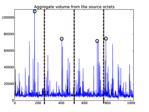
Figure 1: Algorithm 1’s data structure consists of $q=4$ hash arrays of size $m=256$ (here separated by the thick-dashed lines), one for each octet. Circles illustrate the selected maxima of each octet.

IV-B Hashing Pursuit on Sub-streams

Algorithm 2, called Max-Count Hashing Pursuit, is an extension of SHP that minimizes collisions significantly, and hence improves identification accuracy. The idea is to introduce an additional dimension $m^{\prime}$ in our data structure and populate it by using another hash function $h_{t}$. The secondary hash is used to divide the incoming stream into $m^{\prime}$ independent sub-streams (i.e., ‘thin’ the stream).

As stream entries arrive, we initially perform the permutation step discussed above to remove spatial localities. Then, having a uniform hash function $h_{t}:[N]\to[m^{\prime}]$ as discussed in Section III, we apply it on the permuted key $\omega$ to get the index $s$ of the sub-stream. We update the appropriate array entries corresponding to sub-stream $s$ only.

Algorithm 2 Max-Count Hashing Pursuit

0:  Number heavy-hitters: $k$

1:  [Start] Initialize $P_{mc}$ of size $q\times m\times m^{\prime}$.

2:  Perform steps 2 & 3 of Algorithm 1

3:  [Thin] Calculate sub-stream index $s=h_{t}(\omega)$.

4:  [Update] Update $P_{mc}$ for $i\in[q]$:

$$P_{mc}[i,h_{i}\circ\sigma(\omega),s]=P_{mc}[i,h_{i}\circ\sigma(\omega),s]+v,$$

5:  if (Populated $P_{mc}$ for some time window) then

6:     if k==1 then

7:        Construct matrix $P_{max}$ of size $q\times m$, i.e.,

8:        $P_{max}[i,j]=\max_{s}P_{mc}[i,j,s]$,  $i\in[q]$, $j\in[m]$

9:        Find $o_{i}={\rm Argmax}_{j}P_{max}[i,j]$,  $i\in[q]$

10:        [decode] Output $\omega^{*}=\sigma^{-1}(\overline{o_{q}\ldots o_{1}})$.

11:     else

12:        for r=1 to k do

13:           $P_{max}[i,j]=\max_{s\in[m^{\prime}]}P_{mc}[i,j,s]$,  $i\in[q]$, $j\in[m]$

14:           Find $o_{i}={\rm Argmax}_{j}P_{max}[i,j]$,  $i\in[q]$

15:           Find $\ell_{i}={\rm Argmax}_{\ell\in[m^{\prime}]}P_{mc}[i,o_{i},\ell]$,  $i\in[q]$

16:           $P_{mc}[i,o_{i},\ell_{i}]$ = 0,  $i\in[q]$ #Exclude for next iteration

17:           [decode] Output $\omega_{r}^{*}=\sigma^{-1}(\overline{o_{q}\ldots o_{1}})$.

18:        end for

19:     end if

20:  end if

IV-C Hash-thinned MJRTY Boyer-Moore

Algorithm 3 is based on the Boyer-Moore majority vote algorithm [24] (not to be confused with the Boyer-Moore algorithm for string matching used in signature-based detection tools like Snort), and the idea of stream thinning for creating sub-streams described above. The MJRTY Boyer-Moore algorithm can identify exactly the element in stream $\cal{S}$ with the largest traffic assuming that its volume is at least 50% of the total volume (i.e., there is a majority). It solves the problem in time linear in the length of the input sequence and constant memory. In reality, though, a single IP or flow is not usually responsible for such a high fraction of the total volume of the stream. Hence, identification accuracy of the plain Boyer-Moore algorithm could be lacking. To overcome this, we employ the Boyer-Moore idea on sub-streams of $\cal{S}$, constructed as described above. Thus, with, say, $m=256$ sub-streams the ‘majority-threshold’ for each sub-stream becomes $\frac{50}{m}$% ($\approx 0.2$%) of stream $\cal S$ volume. In practice, as Fig. 3 illustrates, this makes the Boyer-Moore-based algorithm to perform remarkably well, but one could use a higher $m$ to further thin stream $\cal{S}$, if needed.

We describe the original Boyer-Moore algorithm with an analogy to the one-dimensional random walk on the line of non-negative integers. A variable $count$ is initialized to $0$ (i.e., the origin) and a candidate variable cand is reserved for use. Once a new IP arrives, we check to see if count is 0. If it is, that IP is set to be the new candidate cand and we move count one step-up, i.e. $count=1$. Otherwise, if the IP is the same as cand, then cand remains unchanged and count is incremented, and, if not, count moves one step-down (decremented). We then proceed to the next IP and repeat the procedure. Provably, when all IPs are read, cand will hold the one with majority, if majority exists.

We implemented a natural extension of the MJRTY Boyer-Moore algorithm to the case of byte and packet counts and applied it in parallel on the sub-streams resulting from hash-thinning. For each sub-stream, we also maintained an additional small and constant size data structure, used to estimate the signal volume.

Algorithm 3 Hash-thinned MJRTY Boyer-Moore

0:  Number heavy-hitters: $k$, $k\leq m$

1:  [Start] Initialize $P_{bm}[i,j]=0$,  $i\in[m]$, $j\in[m^{\prime}]$.

2:  Initialize $count[i]=0$, $cand[i]=-1$,  $i\in[m]$

3:  Upon observing $(\omega,v)$, compute $\sigma(\omega)$.

4:  [Thin] Calculate sub-stream index $s=h_{t}(\omega)$.

5:  [Hash] Compute $j=h\circ\sigma(\omega)$, $h:[N]\to[m^{\prime}]$

6:  [Update]

7:  if $cand[s]==-1$ then

8:     $cand$[s] = $\omega$, $count$[s] = $v$, $P_{bm}$[s,j] = $v$

9:  else

10:     if $cand[s]==\omega$ then

11:        $P_{bm}$[s,j] = $P_{bm}$[s,j] + $v$, $count$[s] = $count$[s] + $v$

12:     else

13:        if $count[s]>0$ then

14:           $count[s]$ = $count[s]$ - $v$

15:           if $count[s]<0$ then

16:              $cand$[s] = $\omega$, $count$[s] = -$count$[s] # reset candidate

17:           end if

18:           $P_{bm}$[s,j] = $P_{bm}$[s,j] + $v$

19:        else

20:           $cand$[s] = $\omega$, $count$[s] = $v$ # reset candidate

21:           $P_{bm}$[s,j] = $P_{bm}$[s,j] + $v$

22:        end if

23:     end if

24:  end if

25:  if (Populated $P_{bm}$ for some time window) then

26:     $P_{est}=\max_{j\in[m^{\prime}]}P_{bm}[i,j]$,  $i\in[m]$

27:     Initialize ${\cal O}=\emptyset$

28:     for r=1 to k do

29:        Find $o={\rm Argmax}_{j\in[m]\setminus{\cal O}}P_{est}[j]$

30:        ${\cal O}={\cal O}\cup o$ #Exclude for next iteration

31:        Output $\omega_{r}^{*}=$cand$[o]$

32:     end for

33:  end if

IV-D Applications to more complex signals

In this section we extend the randomized domain hashing approach to the detection of more complex anomalies. As discussed in Section II, one common scenario could involve a “persistent” user $\omega^{*}$ that accesses abnormally large number of ports. Note that the overall volume or frequency of packets from user $\omega^{*}$ need not be abnormal. Therefore, such anomalous activity may be nearly impossible to detect from algorithms that merely detect large volume hitters. To address this problem with constant and small-size memory, we propose next another algorithm, which combines the randomized hashing and max-stable sketches [25].

These sketches exploit the max-stability property (4) of the Fréchet distribution. Recall that a random variable $Z$ is $1$-Fréchet if $\mathbb{P}\{Z\leq x\}=\exp\{-c/x\}$, for $x>0$, and 0, otherwise, for some scale $\sigma>0$. If $c=1$, then $Z$ is called standard $1$-Fréchet. Let $Z,Z(1),\ldots,Z(n)$ be independent standard 1-Fréchet random variables. Then, it is known [25] that

$$\xi=\max_{1\leq i\leq n}Z(i)\,{\buildrel d\over{=}}\,nZ,$$ (4)

where ‘${\buildrel d\over{=}}$’ denotes equality in distribution. Thus, $\xi$ is a 1-Fréchet variable with scale coefficient $c=n$. One can easily express the median of a 1-Fréchet variable $Z$ with scale coefficient $n$ by considering that $\mathbb{P}\{Z<\rm{med}(Z)\}$ = 1/2. By the definition of the 1-Fréchet distribution and some algebra, one obtains $\rm{med}(Z)=n/{\rm ln}2$.

The theory above can be employed to estimate the number of elements of a set. Specifically, consider the problem of finding the number of unique destinations ports contacted by a given host. When a stream element $(\omega,v)$ arrives, we generate a 1-Fréchet variable with seed that is a function of $v$. Thus, if the same port arrives, the exact pseudo-random number $Z(v)$ is generated. As different ports arrive, we sequentially update our sketch by taking the maximum of the new 1-Fréchet variable and the sketch entry. Essentially, we are building one realization of the $\xi$ random variable described above. The number of different terms $Z(v)$’s will correspond to the number of different ports.

Since, we want to take the median of $\xi$ to estimate the scale coefficient $n$, we independently keep $L$ realizations of the above procedure (see Alg. 4).

Algorithm 4 Max-Stable Hashing Pursuit (MSHP)

0:  Size of max-sketch $L$

1:  [Start] Initialize array $P_{ms}$ of size $q\times m\times L$,

2:  [Permute] Upon observing $(\omega,v)$, compute $\sigma(\omega)$

3:  [Hash] Compute $v_{i}=h_{i}\circ\sigma(\omega),\ i\in[q]$.

4:  [RNG] With random seed $v$, and $\ell\in[L]$, generate $L$ independent 1–Fréchet random variables $Z_{\ell}(v)$.

5:  [Update] Update $P_{ms}$ for $i\in[q]$, $\ell\in[L]$:

$$P_{ms}[i,v_{i},\ell]=\max\{P_{ms}[i,v_{i},\ell],Z_{\ell}(v)\}.$$

6:  if (Populated $P_{ms}$ for some time window) then

7:     Construct matrix $P_{med}$ of size $q\times m$, i.e.,

8:     $P_{med}[i,j]={\rm med}_{\ell}P_{mc}[i,j,\ell]$,  $i\in[q]$ and $j\in[m]$

9:     Find $o_{i}={\rm Argmax}_{j}P_{med}[i,j]$,  $i\in[q]$

10:     [Decode] Output $\omega^{*}=\sigma^{-1}(\overline{o_{q}\ldots o_{1}})$.

11:  end if

V On the accuracy of identification

The proposed algorithms (except the hash-tinned MJRTY Boyer-Moore) are closely related to the general family of sub-linear algorithms in the theoretical work of [16]. Performance guarantees for our algorithms can thus be established in a similar way as for the so-called Euclidean approximate sparse recovery systems of [17].

To understand better the role of collisions, however, we adopt a different approach and provide performance guarantees under the following simplifying assumptions. All proofs are available in the Appendix.

Assumption 1. (exact $k$-sparcity) The signal $f:\Omega\to V$ has precisely $k$ non-zero (non-empty) entries at keys $\omega_{i},\ i\in[k]$.

Assumption 2. (separation) The magnitude functionals $L(i):={\cal L}(f(\omega_{i})),\ i\in[k]$ of the heavy-hitters are all different: $L(1)>L(2)>\cdots>L(k)>0.$ Define $\overline{L}(i):=\sum_{j=i+1}^{k}L(j)$ to be the cumulative magnitude of the bottom $(k-i)$ heavy hitters. By convention set $\overline{L}(k)=0.$

Exact recovery guarantees. Clearly, under Assumption 2, all our algorithms will identify the top-$k$ heavy hitters exactly, provided that there are no hash-collisions. Let $p_{k}(r)$ denote the probability that the top-$r$ heavy hitters are correctly identified for a $k$-sparse signal $f$. The following results provide lower bounds on $p_{k}(r)$ under various conditions.

Theorem 1.

Let $r\in[k]$ and suppose that $L(r)>\overline{L}(r)$. Then, for the Simple Hashing Pursuit algorithm:

$$p_{k}(r) \geq \left(1-\frac{r}{m}\right)^{(k-r)q}\prod_{i=1}^{r-1}\left(1-\frac{i}{m}\right)^{q}$$

$$\geq 1-\frac{qr(k-1)}{2m}.$$

Note: With $\Omega=\{0,1\}^{32}$ and the choice of hash functions as in Section III, we have $q=4$ and $m=256$.

Remark 4 (the birthday problem).

For $r=k$ and $q=1$, the first bound in (1) can be interpreted as the probability that a class of $k$ students have all different birthdays, if the year has $m$ days. It is well-known that this probability decays rather quickly as $k$ grows.

The max-count algorithm addresses this curse of the birthday problem by effectively increasing the value $m$.

Corollary 1.

Under the Assumptions of Proposition 1, for the Max-count Hashing Algorithm, the bounds in (1) apply with $m$ replaced by $m\times m^{\prime}$.

Since the Boyer–Moore algorithm uses one hash function (as opposed to $q$), we obtain the following.

Corollary 2.

Under the Assumptions of Proposition 1, for the hash-thinned MJRTY Boyer-Moore Algorithm, the bounds in (1) apply with $q:=1$.

Bounds on the rate of identification. The exact identification of the top-$r$ hitters is difficult as the above performance bounds indicate since a few collisions may lead to misspecification. Even in the presence of collisions, however, a relatively large proportion of the hitters is identified in practice (see e.g. Fig. 3 below). This suggests examining the rate of identification quantity:

$$e_{rt}(k)=\mathbb{E}N(k)/k,$$ (6)

where $N(k)$ denotes the number of correctly identified heavy hitters among the top $k$. That is, $e_{rt}(k)$ gives the average proportion of identified top hitters.

The combinatorial analysis needed to establish bounds on $e_{rt}(k)$ for the Simple Hashing and Max-count algorithms is rather involved and delegated to a follow-up paper. Under certain conditions, however, an appealing closed-form expression for $e_{rt}(k)$ is available for the hash-thinned MJRTY Boyer-More algorithm. The conditions may be relaxed with the help of technical probabilistic analysis, which merits a separate investigation.

Theorem 2.

Suppose that $L(i)>\overline{L}(i),$ for all $i\in[k]$. Then, under Assumptions 1 & 2, for the hash-thinned MJRTY Boyer-Moore Algorithm, we have the exact expression

$$e_{rt}(k) = \frac{m}{k}\left(1-\left(1-\frac{1}{m}\right)^{k}\right)$$

$$= \frac{m}{k}\left(1-e^{-k/m}(1+O({1}/{m}))\right).$$

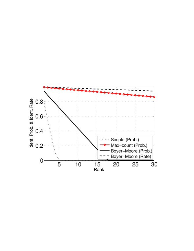
Figure 2: Performance bounds given the Assumptions of Section V.

VI Performance Evaluation

Next, we evaluate our algorithms with Netflow traffic traces provided from the academic ISP Merit Network. The traces are collected at a large edge router. In the hourly-long trace we investigate, our Netflow stream has $\approx 360K$ unique source addresses, $\approx 360K$ unique destinations, and consists of $\approx 4.7$ million flow records. The total volume is $103$ gigabytes and $132$ million packets. We demonstrate results using Python software implementations of our algorithms.

Accuracy performance analysis. Fig. 3 shows the identification accuracy of Algorithms 1–3, compared to the ground truth (obtained by counting using a dynamic hash array, and then sorting). We search for heavy hitters both in byte volume, as well as frequency of occurrence. We use two metrics to evaluate our methods: (i) identification rate and (ii) exact recovery. The first gives the expected proportion of identified heavy hitters among the top-$k$, while the second one is much more strict and measures the probability that all top-$k$ hitters are correctly recovered.

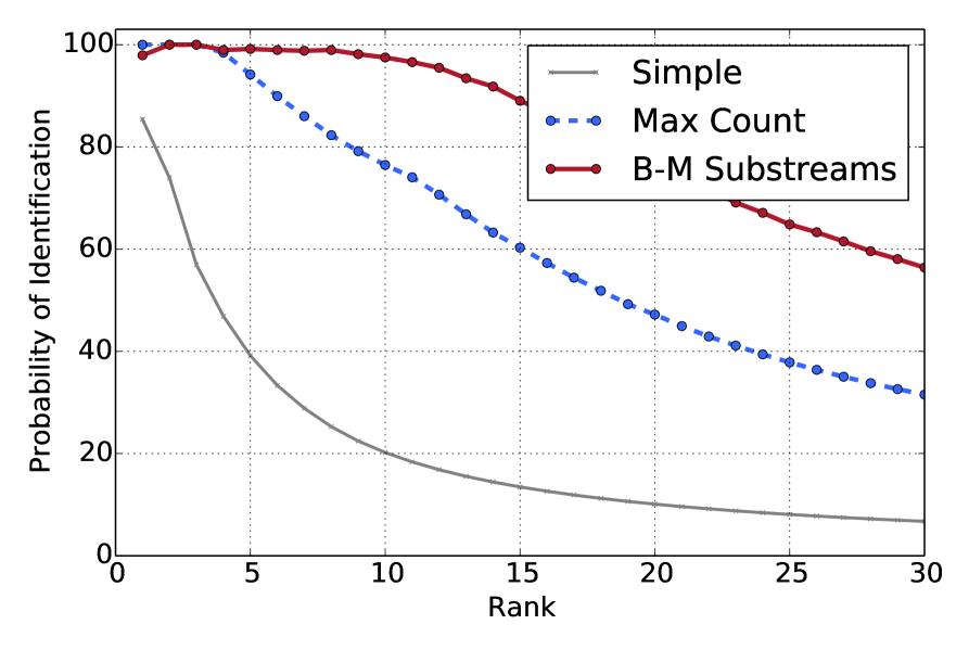
(a) Frequency, ident. rate

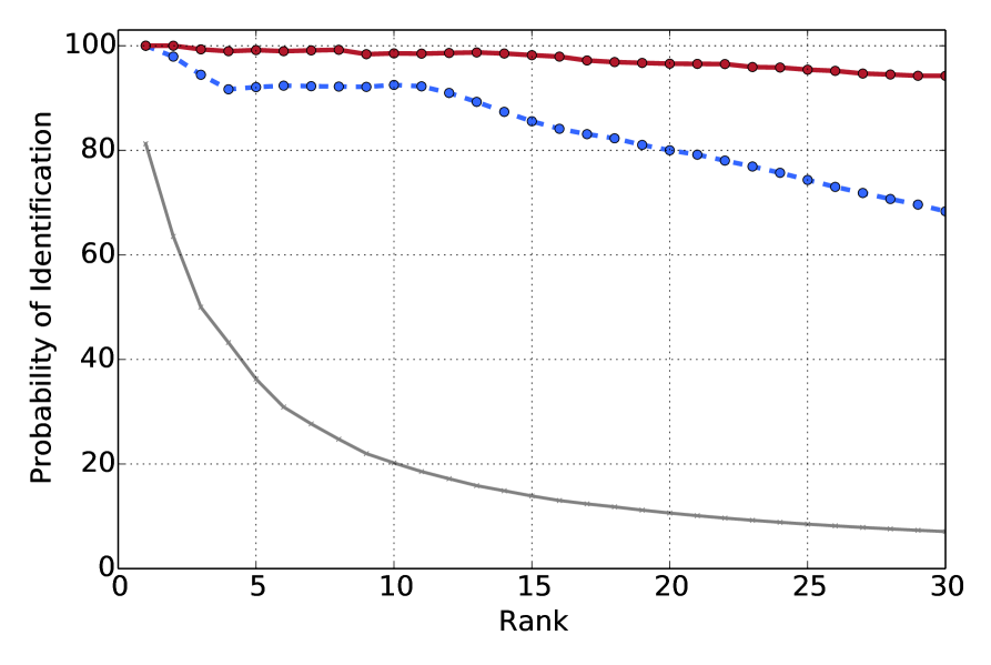
(b) Payload, ident. rate

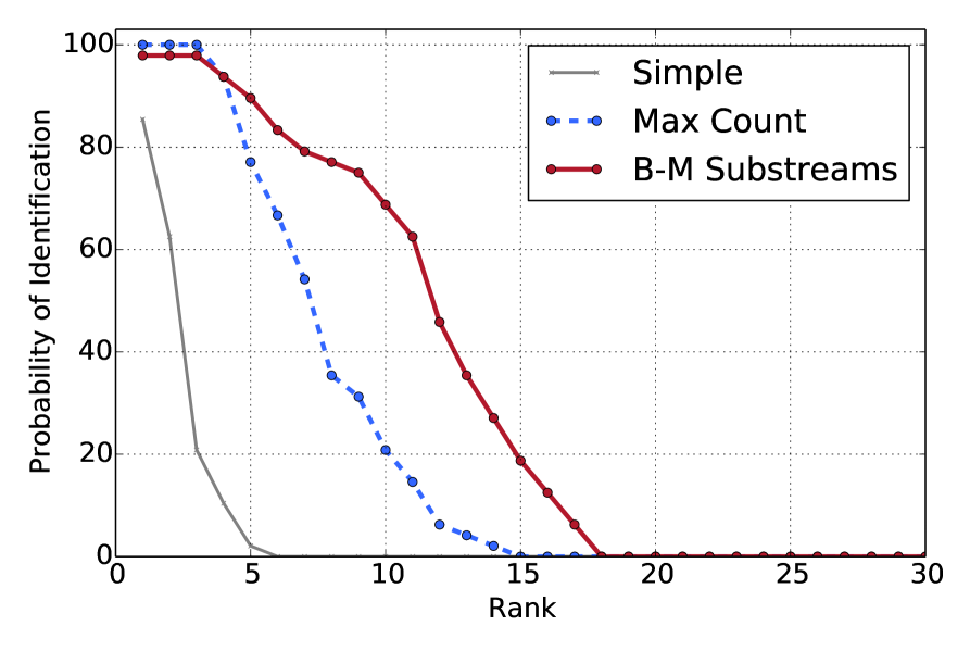
(c) Frequency, exact metric

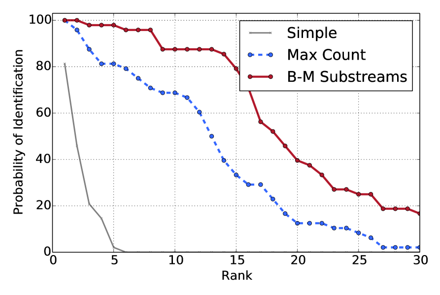
(d) Payload, exact metric

Figure 3: Identification accuracy results (window=100K).

As Fig. 3 depicts, hash-thinned Boyer-Moore and Max-Count perform remarkably well. The window of records we used is $100$K (i.e., we report the culprits every $100$K netflow records), which corresponds (for the stream studied) on the RTS to slots of $~{}1.2$ minutes. The performance of the SHP deteriorates as the number $k$ of top heavy hitters sought increases which is an expected outcome of the birthday problem discussed above. Therefore, SHP is well-suited when stringent memory constraints are imposed, and when only the top-hitter is of interest. Fig. 4 provides a sensitivity analysis w.r.t the window size that one could perform to find the optimal monitoring window size.

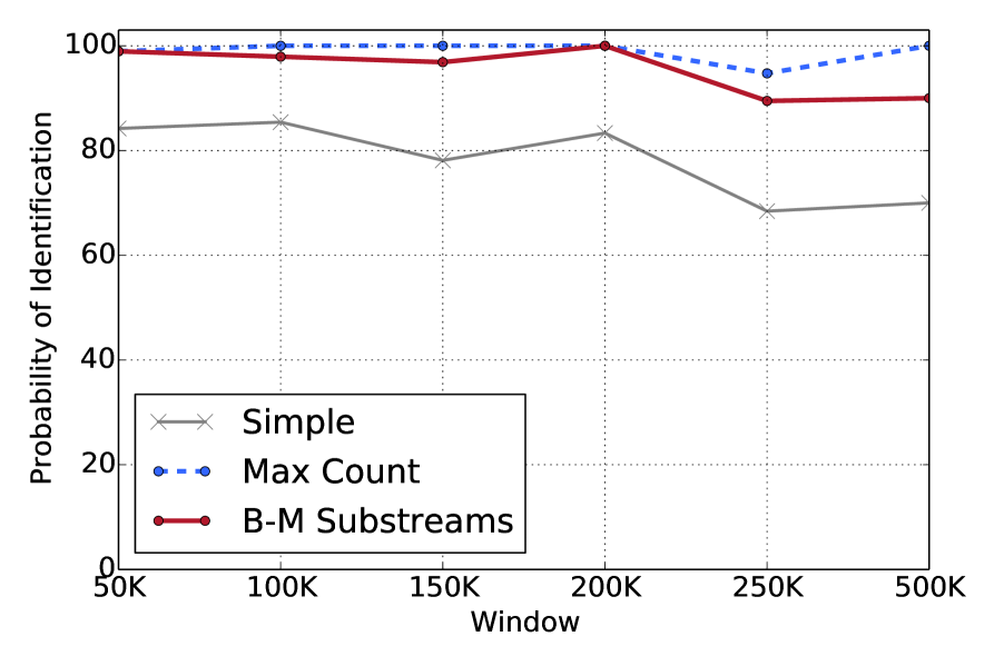
(a) Frequency, top heavy-hitter

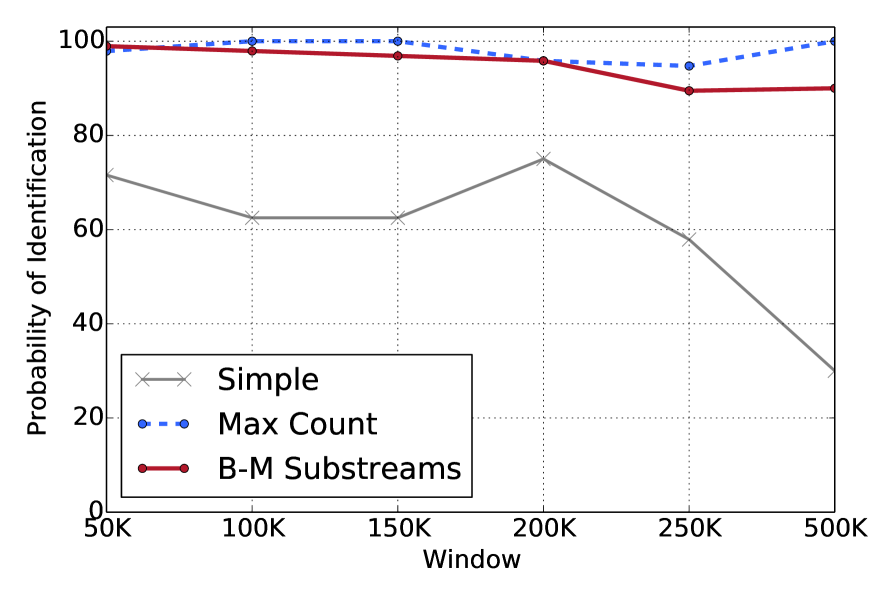
(b) Frequency top-2 hitters

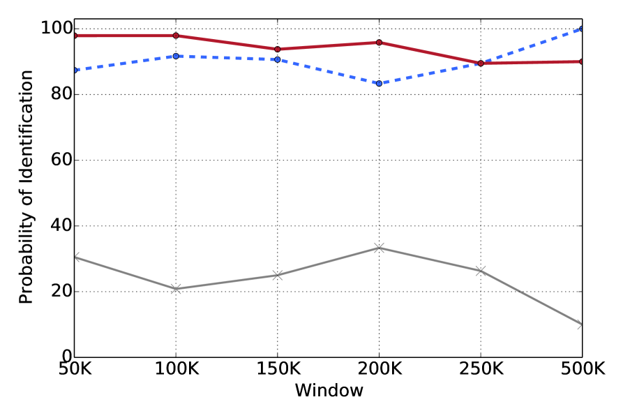
(c) Frequency top-3 hitters

Figure 4: Identification accuracy (using the exact criterion) with varying window.

Table II shows the estimation accuracy of our methods. We juxtapose the actual traffic volume of the heavy-hitter versus an estimate obtain from our sketches. For Algorithms 1 & 2, we estimate the volume by taking the average of the 4 octets of the $m-$ary hash arrays. For thinned Boyer-Moore, we report the value of array $P_{bm}$. Indeed, Algorithm 1’s collisions are inevitable, but for the other two, collisions are spread nicely, and the estimated signal closely approximates the true value (here we round to closest digit). More sophisticated estimates (e.g., see [11] that uses a median-based estimate to boost confidence) can also be considered.

TABLE II: Estimation accuracy (%) of proposed algorithms for top hitter (in bytes) compared to the exact value (window size = 500K).

Time	1	2	3	4	5	6	7	8
Simple	88	88	88	87	93	92	91	62
Max-Count	100	100	100	100	100	100	100	100
Boyer-Moore	100	100	100	100	100	100	100	100

Table III illustrates the small memory requirements of our methods. The Max-Count and Boyer-Moore-based algorithms consume considerably less than 1MB of fast memory, which remains constant. On the other hand, the naïve approach of using a dynamically varying hash-table, has increasing memory requirement. To showcase the memory increase the algorithm was run against a stream with an hourly total byte volume of $1328$ gigabytes. As demonstrated in Table III, as the monitoring window grows (or equivalently, as the amount of traffic increases), memory increases exponentially.

TABLE III: Memory Utilization (in MB)

Window Size ($\times$ 50K)	1	2–7	8–19	20
Exact	.8	3	6	13
Boyer-Moore ($m$=$m^{\prime}$=256)	.5	.5	.5	.5
Max-Count ($q$=4, $m$=256, $m^{\prime}$=50)	.4	.4	.4	.4

Max-Stable sketch case studies. We illustrate Algorithm 4’s accuracy by looking at set-valued signals, tailored for detecting: (i) host scanning, (ii) port scanning, and (iii) a signal based on time to live (TTL) values.

Fig. 5(a) shows the accuracy on host scanning, where the goal is to identify the source IPs that contact large number of destination IPs. A filled-circle on the dotted blue line indicates the occurrences we identify exactly the heavy-hitter IP. The solid gray line shows the exact number of different hosts that the malicious scanner has contacted. The dotted-blue line shows our algorithm’s estimate for the set cardinality obtained by simply averaging, as described above. The identification accuracy is very high, and the misses occur when the set-size is indeed quite small.

In Fig. 5(c), our signal updates involve the set of ports that a given source IP interacts with. Hence, this could be used to identify port scanners. While the accuracy is still quite high, we observe a few mis-identifications. This is because the number of unique ports ($2^{16}$) is much smaller than the unique IPs ($2^{32}$). As a result, collisions in our hash-arrays matter more in this case; background “noise” from non-malicious IPs could alter the ranking of even one of the buckets selected on the identification step, and result in mis-identification.

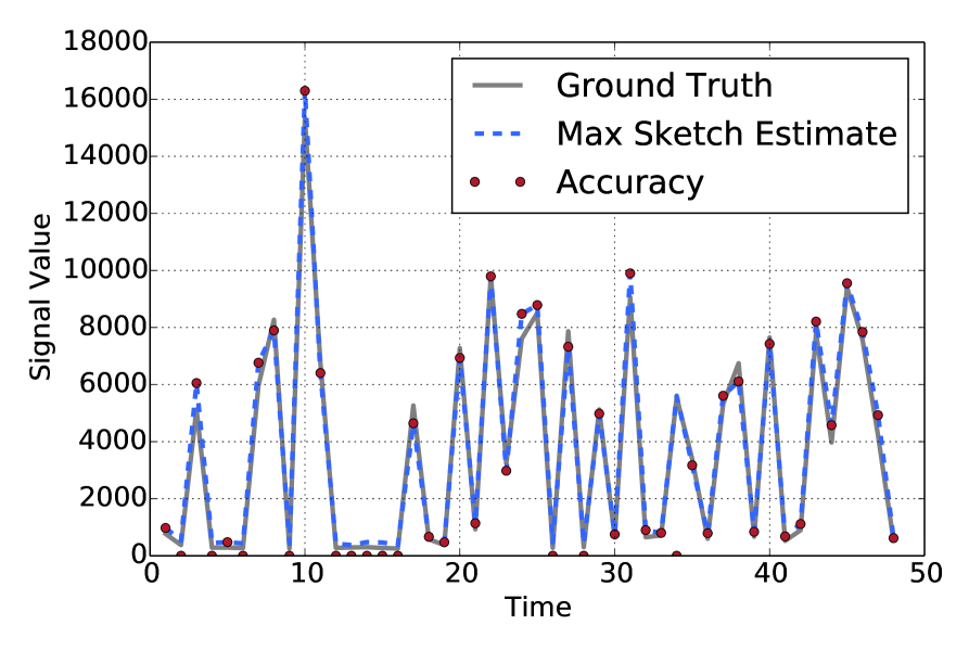
(a) Host scanning

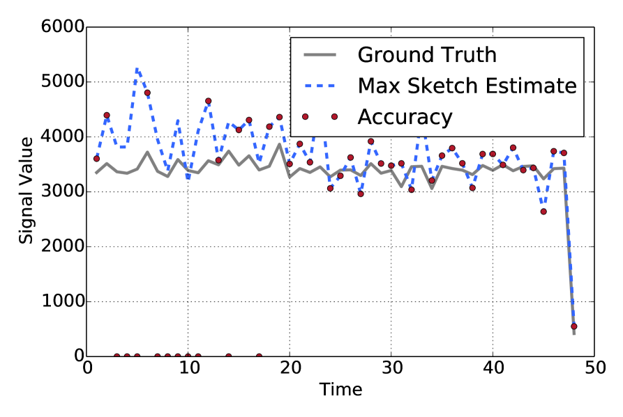
(b) Port scanning

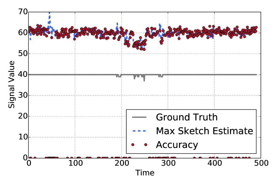
(c) IP spoofing

Figure 5: Evaluation of Algorithm 4 on the Netflow stream (window=100K).

In Fig. 5(c), we apply the max-stable sketch on Darknet data (known also as Internet background radiation) [26]. The dataset available does not include Netflow records, but instead consists of packets captured at a network interface (this 1-hour long trace has $50$ million packets). Darknets are composed of traffic destined at unallocated address spaces (i.e., dark spaces). It is therefore directly associated with malicious acts or misconfigurations. Algorithm 4 is used to identify packets whose source IP has been spoofed. To achieve this we look at the TTL values of each packet. For the problem at hand, a heavy-hitter is a source IP whose set of unique TTL values in the monitoring window is large – an indication of spoofing [27]. The evaluation results illustrate that the culprit is correctly identified in around 84% of the cases, and the result for deteriorating performance is again due to the small cardinality of the unique set of TTL values (which is $2^{8}$ in theory, but in practice less unique TTL values are encountered).

VII Conclusions

We presented a family of algorithms that are well-suited for online implementation in fast network streams. In addition, our framework can be employed to find heavy-hitters on a variety of signals, including complex ones that involve operations with sets. Further, our algorithms are amenable for distributed implementation; in a decentralized setting, the proposed data structures could be constructed at various observation points (i.e., the switch/router) and then transmitted for aggregation at centralized decision centers due to two important properties: (i) they are small and constant in size and, hence, can be efficiently emitted over the network to a centralized location, (ii) they can be linearly combined/aggregated by the centralized worker and reduced to a single sketch object that can be utilized to yield the final culprits.

Appendix A Proofs

A-A Exact recovery guarantees

The proof of Theorem 1 follows.

Proof.

For each hash function $h_{j},\ j\in[q]$, let $A_{j}(r)$ be the event that the top-$r$ heavy hitters are hashed into $r$ different bins, and at the same time, the remaining $k-r$ hitters are hashed into the remaining $m-r$ bins. That is, the bins of the top-$r$ hitters involve no collisions. By the independence of $h_{j}(\omega_{i}),\ i\in[k]$, we have

$$\mathbb{P}(A_{j}(r))=\frac{(m-1)}{m}\cdots\frac{(m-r+1)}{m}\times\left(\frac{m-r}{m}\right)^{k-r}.$$ (8)

If the event $\cap_{j\in[q]}A_{j}(r)$ occurs, then the top-$r$ heavy hitters will be correctly identified. Thus, the independence of the events $A_{j}(r)$ in $j\in[q]$ implies that

$$p_{k}(r)\geq\mathbb{P}(\cap_{j\in[q]}A_{j}(r))=\mathbb{P}(A_{j}(r))^{q},$$

which by (1) yields the first bound. The second bound follows from the product comparison inequality

$$|\prod_{i=1}^{k}a_{i}-\prod_{i=1}^{k}b_{i}|\leq\sum_{i=1}^{k}|a_{i}-b_{i}|,$$

valid for all $a_{i},b_{i}\in[-1,1]$. Indeed, setting $a_{i}=1$ and $b_{i}=(m-i\wedge r)/m$, we get

$$1-\mathbb{P}(A_{j}(r))^{q} \leq q\sum_{i=1}^{r-1}\frac{i}{m}+(k-r)\frac{r}{m}$$

$$= q\frac{r(r-1)+(k-r)r}{2m},$$

which gives the second bound. ∎

For Corollary 1, we have:

Proof.

The result follows by observing that hash-thinning with an independent uniform hash function $h^{(s)}$ taking $m$ values leads to $m^{2}$ bins in (8). ∎

A-B Bounds on the rate of identification

The proof of Theorem 2 is as follows.

Proof.

The assumption $L(i)>\overline{L}(i)$ guarantees that $N(k)$ equals the number of distinct values in the set of hashes $\{h(\omega_{1}),\cdots,h(\omega_{k})\}$. Let $Y_{i}=1$ if bin $i$ is occupied and $0$ otherwise, for $i\in[m].$ Observe that

$$\mathbb{E}N(k)=\sum_{i=1}^{m}\mathbb{E}Y_{i}=m\mathbb{E}Y_{1},$$ (9)

by exchangeability. Note, however, that

$$\mathbb{E}Y_{1}=1-\mathbb{P}(h(\omega_{j})\not=1,\ j\in[k])=1-\left(1-\frac{1}{m}\right)^{k},$$

since $h(\omega_{i}),\ i\in[k]$ are independent and Uniform$([m])$.

This, in view of (6) and (9), implies the first relation in (2). The second follows from the standard approximation $(1-1/m)^{m}\approx e^{-1}.$ ∎

References

- [1] C. Rossow, “Amplification Hell: Revisiting Network Protocols for DDoS Abuse,” in 2014 Network and Distributed System Security Symposium, NDSS, San Diego, CA, 2014.
- [2] A. Lakhina, M. Crovella, and C. Diot, “Diagnosing network-wide traffic anomalies,” SIGCOMM Comput. Commun. Rev., vol. 34, pp. 219–230, August 2004.
- [3] P. Barford, J. Kline, D. Plonka, and A. Ron, “A signal analysis of network traffic anomalies,” in 2nd ACM SIGCOMM Workshop on Internet measurement, NY, USA, 2002, pp. 71–82.
- [4] T. Idé, “Eigenspace-based anomaly detection in computer systems,” in 10th ACM SIGKDD (KDD), 2004, pp. 440–449.
- [5] J. Zhang, J. Rexford, and J. Feigenbaum, “Learning-based anomaly detection in BGP updates,” in 2005 ACM SIGCOMM MineNet, NY, USA, 2005, pp. 219–220.
- [6] M. Thottan, G. Liu, and C. Ji, “Anomaly detection approaches for communication networks,” in Algorithms for Next Generation Networks, 2010, pp. 239–261.
- [7] G. Cormode and S. Muthukrishnan, “An improved data stream summary: the count-min sketch and its applications,” J. Algorithms, vol. 55, no. 1, pp. 58–75, Apr. 2005.
- [8] G. Cormode, F. Korn, S. Muthukrishnan, and D. Srivastava, “Finding hierarchical heavy hitters in data streams,” in VLDB ’03, 2003, pp. 464–475.
- [9] G. Cormode, T. Johnson, F. Korn, S. Muthukrishnan, O. Spatscheck, and D. Srivastava, “Holistic UDAFs at streaming speeds,” in ACM SIGMOD, NY, USA, 2004, pp. 35–46.
- [10] A. C. Gilbert, M. J. Strauss, J. A. Tropp, and R. Vershynin, “Algorithmic linear dimension reduction in the ℓ1 norm for sparse vectors,” in Allerton 2006, 2006.
- [11] B. Krishnamurthy, S. Sen, Y. Zhang, and Y. Chen, “Sketch-based change detection: methods, evaluation, and applications,” in 3rd ACM SIGCOMM IMC, NY, USA, 2003, pp. 234–247.
- [12] R. Schweller, Z. Li, Y. Chen, Y. Gao, A. Gupta, Y. Zhang, P. Dinda, M.-Y. Kao, and G. Memik, “Reverse hashing for high-speed network monitoring: Algorithms, evaluation, and applications,” in INFOCOM 2006, 2006, pp. 1–12.
- [13] G. Cormode and S. Muthukrishnan, “What’s new: finding significant differences in network data streams,” in INFOCOM 2004, vol. 3, 2004, pp. 1534–1545 vol.3.
- [14] Y. Gao, Z. Li, and Y. Chen, “A DoS Resilient Flow-level Intrusion Detection Approach for High-speed Networks,” in International Conference on Distributed Computing Systems, 2006, pp. 39–39.
- [15] G. Cormode and S. Muthukrishnan, “What’s hot and what’s not: Tracking most frequent items dynamically,” ACM Trans. Database Syst., vol. 30, no. 1, pp. 249–278, Mar. 2005.
- [16] E. Porat and M. J. Strauss, “Sublinear time, measurement-optimal, sparse recovery for all,” in ACM-SIAM SODA, 2012, pp. 1215–1227.
- [17] A. Gilbert, Y. Li, E. Porat, and M. Strauss, “Approximate sparse recovery: Optimizing time and measurements,” SIAM Journal on Computing, vol. 41, no. 2, pp. 436–453, 2012.
- [18] S. Muthukrishnan, “Data streams: Algorithms and applications,” Found. Trends Theor. CS, vol. 1, no. 2, pp. 117–236, Aug. 2005.
- [19] J. Tropp and A. Gilbert, “Signal recovery from random measurements via orthogonal matching pursuit,” Information Theory, IEEE Transactions on, vol. 53, no. 12, pp. 4655–4666, Dec 2007.
- [20] A. C. Gilbert, M. J. Strauss, J. A. Tropp, and R. Vershynin, “One sketch for all: Fast algorithms for compressed sensing,” in STOC ’07, NY, USA, 2007, pp. 237–246.
- [21] D. Donoho, “Compressed sensing,” Information Theory, IEEE Transactions on, vol. 52, no. 4, pp. 1289–1306, April 2006.
- [22] P. Indyk, “Explicit constructions for compressed sensing of sparse signals,” in 19-th ACM-SIAM SODA. PA, USA: Society for Industrial and Applied Mathematics, 2008, pp. 30–33.
- [23] S. Halevi, “Invertible universal hashing and the TET encryption mode,” in Advances in Cryptology - CRYPTO 2007, ser. Lecture Notes in CS, A. Menezes, Ed., 2007, vol. 4622, pp. 412–429.
- [24] R. Boyer and J. Moore, “MJRTY - a fast majority vote algorithm,” in Automated Reasoning, ser. Automated Reasoning Series, R. Boyer, Ed., 1991, vol. 1, pp. 105–117.
- [25] S. Stoev, M. Hadjieleftheriou, G. Kollios, and M. Taqqu, “Norm, point, and distance estimation over multiple signals using max-stable distributions,” in IEEE 23rd International Conference on Data Engineering, April 2007, pp. 1006–1015.
- [26] E. Wustrow, M. Karir, M. Bailey, F. Jahanian, and G. Houston, “Internet Background Radiation Revisited,” in 10th ACM SIGCOMM IMC, Melbourne, Australia, November 2010.
- [27] R. Beverly and S. Bauer, “The spoofer project: Inferring the extent of source address filtering on the internet,” in SRUTI’05. Berkeley, CA, USA: USENIX Association, 2005, pp. 8–8.