On a class of generalized Takagi functions
with linear pathwise quadratic variation

Abstract

We consider a class $\mathscr{X}$ of continuous functions on $[0,1]$ that is of interest from two different perspectives. First, it is closely related to sets of functions that have been studied as generalizations of the Takagi function. Second, each function in $\mathscr{X}$ admits a linear pathwise quadratic variation and can thus serve as an integrator in Föllmer’s pathwise Itō calculus. We derive several uniform properties of the class $\mathscr{X}$. For instance, we compute the overall pointwise maximum, the uniform maximal oscillation, and the exact uniform modulus of continuity for all functions in $\mathscr{X}$. Furthermore, we give an example of a pair $x,y\in\mathscr{X}$ for which the quadratic variation of the sum $x+y$ does not exist.

Mathematics Subject Classification 2010: 26A30, 26A15, 60H05, 26A45

Key words: Generalized Takagi function, Takagi class, uniform modulus of continuity, pathwise quadratic variation, pathwise covariation, pathwise Itō calculus, Föllmer integral

1 Introduction

In this note, we study a class ${\mathscr{X}}$ of continuous functions on $[0,1]$ that is of interest from several different perspectives. On the one hand, just as typical Brownian sample paths, each function $x\in{\mathscr{X}}$ admits the linear pathwise quadratic variation, $\langle x\rangle_{t}=t$, in the sense of Föllmer [13] and therefore can serve as an integrator in Föllmer’s pathwise Itō calculus. On the other hand, ${\mathscr{X}}$ is a subset, or has a nonempty intersection, with classes of functions that have been studied as generalizations of Takagi’s celebrated example [29] of a nowhere differentiable continuous function. We will now explain the connections of our results with these two separate strands of literature.

1.1 Contributions to Föllmer’s pathwise Itō calculus

In 1981, Föllmer [13] proposed a pathwise version of Itō’s formula, which, as a consequence, yields a strictly pathwise definition of the Itō integral as a limit of Riemann sums. Some recent developments have led to a renewed interest in this pathwise approach. Among these is the conception of functional pathwise Itō calculus by Dupire [10] and Cont and Fournié [6, 7], which for instance is crucial in defining partial differential equations on path space [11]. Another source for the renewed interest in pathwise Itō calculus stems from the growing awareness of model ambiguity in mathematical finance and the resulting desire to reduce the reliance on probabilistic models; see, e.g., [15] for a recent survey and [3, 4, 8, 14, 26, 27] for case studies with successful applications of pathwise Itō calculus to financial problems. A systematic introduction to pathwise Itō calculus, including an English translation of [13], is provided in [28].

A function $x\in C[0,1]$ can serve as an integrator in Föllmer’s pathwise Itō calculus if it admits a continuous pathwise quadratic variation $t\mapsto\langle x\rangle_{t}$ along a given refining sequence of partitions of $[0,1]$. This condition is satisfied whenever $x$ is a sample path of a continuous semimartingale, such as Brownian motion, and does not belong to a certain nullset. This nullset, however, is generally not known explicitly, and so it is not possible to tell whether a specific realization $x$ of Brownian motion does indeed admit a continuous pathwise quadratic variation. The first purpose of this note is to provide a rich class ${\mathscr{X}}$ of continuous functions that can be constructed in a straightforward manner and that do admit the nontrivial pathwise quadratic variation $\langle x\rangle_{t}=t$ for all $x\in{\mathscr{X}}$. The functions in ${\mathscr{X}}$ can thus be used as a class of test integrators in pathwise Itō calculus. Our corresponding result, Proposition 2.6, slightly extends a previous result by Gantert [18, 19], from which it follows that $\langle x\rangle_{1}=1$ for all $x\in{\mathscr{X}}$.

Still within this context, a second purpose of this note is to investigate whether the existence of $\langle x\rangle$ and $\langle y\rangle$ implies the existence of $\langle x+y\rangle$ (or, equivalently, the existence of the pathwise quadratic covariation $\langle x,y\rangle$). For typical sample paths of a continuous semimartingale, this implication is always true, but the corresponding nullset will depend on both $x$ and $y$. In the literature on pathwise Itō calculus, however, it has been taken for granted that the existence of $\langle x+y\rangle$ cannot be deduced from the existence of $\langle x\rangle$ and $\langle y\rangle$. In Proposition 2.7 we will now give an example of two functions $x,y\in{\mathscr{X}}$ for which $\langle x+y\rangle$ does indeed not exist. To the knowledge of the author, such an example has so far been missing from the literature.

1.2 Contributions to the theory of generalized Takagi functions

In 1903, Takagi [29] proposed an example of a continuous function on $[0,1]$ that is nowhere differentiable. This function has since been rediscovered several times and its properties have been studied extensively; see the recent surveys by Allaart and Kawamura [2] and Lagarias [24]. While the original Takagi function itself does not belong to our class ${\mathscr{X}}$, there are at least two classes of functions whose study was motivated by the Takagi function and that are intimately connected with ${\mathscr{X}}$. One family of functions is the “Takagi class” introduced in 1984 by Hata and Yamaguti [20]. Similar but more restrictive function classes were introduced earlier by Faber [12] or Kahane [21]. The Takagi class has a nonempty intersection with ${\mathscr{X}}$ but neither one is included in the other. More recently, Allaart [1] extended the Takagi class to a more flexible class of functions. This family now contains ${\mathscr{X}}$. By extending arguments given by Kôno [23] for the Takagi class, Allaart [1] studies in particular the moduli of continuity of certain functions in his class.

In contrast to these previous studies, the focus of this paper is not so much on the individual features of functions $x\in{\mathscr{X}}$ but rather on uniform properties of the entire class ${\mathscr{X}}$. Here we compute the overall pointwise maximum, the uniform maximal oscillation, and the exact uniform modulus of continuity for all functions in ${\mathscr{X}}$. In these computations, we cannot use previous methods that were conceived for the analysis of the Takagi functions and its generalizations. For instance, neither the result and arguments from Kôno [23] nor the ones from Allaart [1] apply to the modulus of continuity of functions in ${\mathscr{X}}$, and a suitable extension of the previous approaches must be developed. This new extension exploits the self-similar structure of ${\mathscr{X}}$ and its members.

A special role in our analysis will be played by the function $\widehat{x}$, defined in (2.2) below. It has previously appeared in the work of Ledrappier [25], who studied the Hausdorff dimension of its graph, and in Gantert [18, 19]. Here we will determine its global maximum and its exact modulus of continuity. In particular the results on the global maximum of $\widehat{x}$ will be needed in our analysis of the uniform properties of ${\mathscr{X}}$, but these results are also interesting in their own right.

This paper is organized as follows. In the subsequent Section 2 we first introduce our class ${\mathscr{X}}$ and then discuss its uniform properties in Theorems 2.2 and 2.3 and Corollary 2.5. We then recall Föllmer’s [13] notions of pathwise quadratic variation and covariation and state our corresponding results. All proofs are given in Section 3.

2 Statement of results

Recall that the Faber–Schauder functions are defined as

$$e_{\emptyset}(t):=t,\qquad e_{0,0}(t):=(\min\{t,1-t\})^{+},\qquad e_{m,k}(t):=2^{-m/2}e_{0,0}(2^{m}t-k)$$

for $t\in{\mathbb{R}}$, $m=1,2,\dots$, and $k\in\mathbb{Z}$. The graph of $e_{m,k}$ looks like a wedge with height $2^{-\frac{m+2}{2}}$, width $2^{-m}$, and center at $t=(k+\frac{1}{2})2^{-m}$. In particular, the functions $e_{m,k}$ have disjoint support for distinct $k$ and fixed $m$. Now let coefficients $\theta_{m,k}\in\{-1,+1\}$ be given and define for $n\in\mathbb{N}$ the continuous functions

$$x^{n}(t):=\sum_{m=0}^{n-1}\sum_{k=0}^{2^{m}-1}\theta_{m,k}e_{m,k}(t),\qquad 0\leq t\leq 1.$$ (2.1)

It is well known (see, e.g., [1]) and easy to see that, due the uniform boundedness of the coefficients $\theta_{m,k}$, the functions $x^{n}(t)$ converge uniformly in $t$ to a continuous function $x(t)$ as $n\uparrow\infty$. Let us denote by

$${\mathscr{X}}:=\Big{\{}x\in C[0,1]\,\Big{|}\,x=\sum_{m=0}^{\infty}\sum_{k=0}^{2^{m}-1}\theta_{m,k}e_{m,k}\text{ for coefficients }\theta_{m,k}\in\{-1,+1\}\Big{\}}$$

the class of limiting functions arising in this way. A function $x\in{\mathscr{X}}$ belongs to the “Takagi class” introduced by Hata and Yamaguti [20] if and only if the coefficients $\theta_{m,k}$ in (2.1) are independent of $k$. Moreover, ${\mathscr{X}}$ is a subset of the more flexible class of generalized Takagi functions studied by Allaart [1]. The original Takagi function, however, is obtained by taking $\theta_{m,k}=2^{-m/2}$ and therefore does not belong to ${\mathscr{X}}$.

Remark 2.1 (On similarities with Brownian sample paths).

The functions in ${\mathscr{X}}$ can exhibit interesting fractal structures; see Figure 1. Figure 2, on the other hand, displays some similarities with the sample paths of a Brownian bridge. This similarity is not surprising since the well-known Lévy–Ciesielski construction of the Brownian bridge consists in replacing the coefficients $\theta_{m,k}\in\{-1,+1\}$ with independent standard normal random variables (see, e.g., [22]). As a matter of fact, using arguments of de Rham [9] and Billingsley [5], it was shown in [1, Theorem 3.1 (iii)] that functions in ${\mathscr{X}}$ share with Brownian sample paths the property of being nowhere differentiable. Moreover, Ledrappier [25] showed that the Hausdorff dimension of the graph of the function

$$\widehat{x}:=\sum_{m=0}^{\infty}\sum_{k=0}^{2^{m}-1}e_{m,k}$$ (2.2)

is the same as that of the graphs of typical Brownian trajectories, namely $3/2$. In Proposition 2.6 we will see, moreover, that the functions in ${\mathscr{X}}$ have the same pathwise quadratic variation as Brownian sample paths.

Our first result is concerned with (uniform) maxima and oscillations of the functions in ${\mathscr{X}}$. It will also be concerned with the function $\widehat{x}$ defined in (2.2), a function that will play a special role throughout our analysis. The maximum of the original Takagi function was computed by Kahane [21], but his method does not apply in our case, and more complex arguments are needed here.

\begin{overpic}[width=227.62204pt]{graphics/Mount_Takagi_Max_16.pdf} \put(31.0,0.0){\scriptsize{1/3}} \put(47.0,0.0){\scriptsize{1/2}} \put(63.0,0.0){\scriptsize{2/3}} \put(96.0,0.0){\scriptsize{1}} \put(-5.0,31.0){\scriptsize{1/2}} \put(-1.0,57.0){\scriptsize{1}} \put(-16.0,64.0){\scriptsize{$\frac{1}{3}(2+\sqrt{2})$}} \end{overpic}

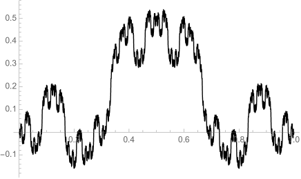
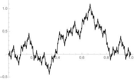
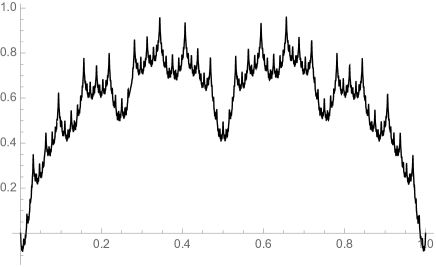
Figure 1: Plots of functions in ${\mathscr{X}}$ for various choices of $\theta_{m,k}$. The upper left-hand panel shows the function $\widehat{x}$, which is defined through $\theta_{m,k}=1$, together with its global maximum. The upper right-hand panel corresponds to $\theta_{m,k}=(-1)^{m}$, the lower left-hand panel to $\theta_{m,k}=(-1)^{m+k}$, and the lower right-hand panel to $\theta_{m,k}=(-1)^{\lfloor m/5\rfloor}$.

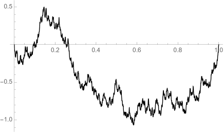
Figure 2: Plots of $x\in{\mathscr{X}}$ when the coefficients $\theta_{m,k}$ form an independent and identically distributed $\{-1,+1\}$-valued random sequence such that $\theta_{m,k}=+1$ with probability $\frac{1}{2}$ (left) and $\frac{1}{4}$ (right). The dashed line corresponds to the approximation $\langle x\rangle^{8}$ of the quadratic variation along the $8^{\text{th}}$ dyadic partition $\mathbb{T}_{8}$.

Theorem 2.2 (Uniform maximum and oscillations).

The class ${\mathscr{X}}$ has the following uniform properties.

1. The uniform maximum of functions in ${\mathscr{X}}$ is attained by $\widehat{x}$ and given by

   $$\max_{x\in{\mathscr{X}}}\max_{t\in[0,1]}|x(t)|=\max_{t\in[0,1]}\widehat{x}(t)=\frac{1}{3}(2+\sqrt{2}).$$

   Moreover, the maximum of $\widehat{x}(t)$ is attained at $t=\frac{1}{3}$ and $t=\frac{2}{3}$.

2. The maximal uniform oscillation of functions in ${\mathscr{X}}$ is

   $$\max_{x\in{\mathscr{X}}}\max_{s,t\in[0,1]}|x(t)-x(s)|=\frac{1}{6}(5+4{\sqrt{2}}),$$

   where the respective maxima are attained at $s=1/3$, $t=5/6$, and

   $$x^{*}:=e_{0,0}+\sum_{m=1}^{\infty}\bigg{(}\sum_{k=0}^{2^{m-1}-1}e_{m,k}-\sum_{\ell=2^{m-1}}^{2^{m}-1}e_{m,\ell}\bigg{)};$$ (2.3)

We refer to Figure 6 for a plot of the function $x^{*}$.

In our next result, we will investigate the modulus of continuity of $\widehat{x}$ and the uniform modulus of continuity of the class ${\mathscr{X}}$. Kôno [23] analyzed the moduli of continuity for some functions in the Takagi class of Hata and Yamaguti [20], and Allaart [1] later extended this result. However, neither the result and arguments from [23] nor the ones from [1] apply to the functions in ${\mathscr{X}}$, because the sequence $a_{m}:=2^{m/2}$ is not bounded. To state our results, let us denote by

$$\nu(h):=\lfloor-\log_{2}h\rfloor,\qquad h>0,$$ (2.4)

the integer part of $\log_{2}\frac{1}{h}$, and define

$$\omega(h) :=\Big{(}1+\frac{1}{\sqrt{2}}\Big{)}h2^{\nu(h)/2}+\frac{1}{3}(\sqrt{8}+2)2^{-\nu(h)/2}.$$

Note that $\omega(h)$ is of the order $O(\sqrt{h})$ as $h\downarrow 0$. More precisely,

$$\liminf_{h\downarrow 0}\frac{\omega(h)}{\sqrt{h}}=2\sqrt{\frac{4}{3}+\sqrt{2}},\qquad\qquad \limsup_{h\downarrow 0}\frac{\omega(h)}{\sqrt{h}}=\frac{1}{6}(11+7\sqrt{2}).$$

These exact limits will however not be needed in the remainder of the paper.

Theorem 2.3 (Moduli of continuity).

1. The function $\widehat{x}$ has $\omega$ as its modulus of continuity. More precisely,

   $$\limsup_{h\downarrow 0}\max_{0\leq t\leq 1-h}\frac{|\widehat{x}(t+h)-\widehat{x}(t)|}{\omega(h)}=1.$$

2. An exact uniform modulus of continuity for functions in ${\mathscr{X}}$ is given by $\sqrt{2}\omega$. That is,

   $$\limsup_{h\downarrow 0}\sup_{x\in{\mathscr{X}}}\max_{0\leq t\leq 1-h}\frac{|x(t+h)-x(t)|}{\omega(h)}=\sqrt{2}.$$

   Moreover, the above supremum over functions $x\in{\mathscr{X}}$ is attained by the function $x^{*}$ defined in (2.3) in the sense that

   $$\limsup_{h\downarrow 0}\max_{0\leq t\leq 1-h}\frac{|x^{*}(t+h)-x^{*}(t)|}{\omega(h)}=\sqrt{2}.$$

Remark 2.4.

In the proof of Theorem 2.3, we will actually show the following upper bounds that are stronger than the corresponding statements in the theorem:

$$|\widehat{x}(t+h)-\widehat{x}(t)|\leq\omega(h)\qquad\text{and}\qquad\sup_{x\in{\mathscr{X}}}|x(t+h)-x(t)|\leq\sqrt{2}\omega(h)$$

for all $h\in[0,1)$ and $t\in[0,1-h]$.

Corollary 2.5.

${\mathscr{X}}$ is a compact subset of $C[0,1]$ with respect to the topology of uniform convergence.

Theorem 2.3 (b) implies moreover that each $x\in{\mathscr{X}}$ is Hölder continuous with exponent $\frac{1}{2}$ and hence admits a finite 2-variation in the sense that

$$\sup_{\mathbb{T}}\sum_{t\in\mathbb{T}}(x(t^{\prime})-x(t))^{2}<\infty,$$ (2.5)

where the supremum is taken over all partitions $\mathbb{T}$ of $[0,1]$ and $t^{\prime}$ denotes the successor of $t$ in $\mathbb{T}$, i.e.,

$$t^{\prime}=\begin{cases}\min\{u\in\mathbb{T}\,|\,u>t\}&\text{if $t<1$,}\\ 1&\text{if $t=1$.}\end{cases}$$

Each $x\in{\mathscr{X}}$ can therefore serve as an integrator in the pathwise integration theory of rough paths; see, e.g., Friz and Hairer [17]. A different pathwise integration theory was proposed earlier by Föllmer [13]. It is based on the following notion of pathwise quadratic variation. Instead of considering the supremum over all partitions as in (2.5), one fixes an increasing sequence of partitions $\mathbb{T}_{1}\subset\mathbb{T}_{2}\subset\cdots$ of $[0,1]$ such that the mesh of $\mathbb{T}_{n}$ tends to zero; such a sequence $(\mathbb{T}_{n})_{n\in\mathbb{N}}$ will be called a refining sequence of partitions. For $x\in C[0,1]$ one then defines the sequence

$$\langle x\rangle_{t}^{n}:=\sum_{s\in\mathbb{T}_{n},\,s\leq t}(x(s^{\prime})-x(s))^{2}.$$ (2.6)

The function $x\in C[0,1]$ is said to admit the continuous quadratic variation $\langle x\rangle$ along the sequence $(\mathbb{T}_{n})$ if for all $t\in[0,1]$ the limit

$$\langle x\rangle_{t}:=\lim_{n\uparrow\infty}\langle x\rangle^{n}_{t}$$ (2.7)

exists, and if $t\mapsto\langle x\rangle_{t}$ is a continuous function. Föllmer’s pathwise Itō calculus uses this class of functions $x$ as integrators.

For given $x\in C[0,1]$, the approximations $\langle x\rangle^{n}_{t}$ are typically not monotone in $n$, and so it is not clear a priori whether the limit in (2.7) exists. Moreover, even if the limit exists, it may depend strongly on the particular choice of the underlying sequence of partitions. For instance, it is known that for any $x\in C[0,1]$ there exists a refining sequence $(\mathbb{T}_{n})_{n\in\mathbb{N}}$ of partitions such that the quadratic variation of $x$ along $(\mathbb{T}_{n})_{n\in\mathbb{N}}$ vanishes identically; see [16, p. 47]. It is also not difficult to construct $x\in C[0,1]$ for which the limit in (2.7) exists but satisfies $\langle x\rangle_{t}={\mathbbmss{1}}_{{}_{\scriptstyle]1/2,1]}}(t)$ and is hence discontinuous. On the other hand, it is easy to see that the quadratic variation of a continuous function with bounded variation exists and vanishes along every refining sequence of partitions. Functions that do admit a nontrivial quadratic variation for some refining sequence of partitions must hence be of infinite total variation.

So the first question that arises in this context is how one can obtain functions that do admit a continuous quadratic variation along a given refining sequence of partitions, $(\mathbb{T}_{n})_{n\in\mathbb{N}}$? Of course one can take all sample paths of a Brownian motion (or, more generally, of a continuous semimartingale) that are not contained in a certain null set $A$. But $A$ is generally not given explicitly, and so it is not possible to tell whether a specific realization $x$ of Brownian motion does indeed admit the quadratic variation $\langle x\rangle_{t}=t$ along $(\mathbb{T}_{n})_{n\in\mathbb{N}}$. Moreover, this selection principle for functions $x$ lets a probabilistic model enter through the backdoor, although the initial purpose of pathwise Itō calculus was to get rid of probabilistic models altogether.

In the following proposition, we show that each $x\in{\mathscr{X}}$ admits the linear pathwise quadratic variation $\langle x\rangle_{t}=t$ for $t\in[0,1]$ along the sequence of dyadic partitions:

$$\mathbb{T}_{n}:=\{k2^{-n}\,|\,k=0,\dots,2^{n}\},\qquad n=1,2,\dots$$ (2.8)

This slightly extends a result by Gantert [18, 19], from which it follows that $\langle x\rangle_{1}=1$ for all $x\in{\mathscr{X}}$. Our proposition implies that each $x\in{\mathscr{X}}$ can serve as an integrator in Föllmer’s pathwise Itō calculus.

Proposition 2.6.

Every $x\in{\mathscr{X}}$ admits the quadratic variation $\langle x\rangle_{t}=t$ along the sequence $(\mathbb{T}_{n})$ from (2.8).

The second question that we will address in this context is concerned with a standard assumption that is made in pathwise Itō calculus whenever the covariation of two functions $x,y\in C[0,1]$ is needed. Let

$$\langle x,y\rangle_{t}^{n}:=\sum_{s\in\mathbb{T}_{n},\,s\leq t}(x(s^{\prime})-x(s))(y(s^{\prime})-y(s))$$ (2.9)

and observe that

$$\langle x,y\rangle_{t}^{n}=\frac{1}{2}\Big{(}\langle x+y\rangle_{t}^{n}-\langle x\rangle_{t}^{n}-\langle y\rangle_{t}^{n}\Big{)}.$$ (2.10)

If $x$ and $y$ admit the continuous quadratic variations $\langle x\rangle$ and $\langle y\rangle$ along $(\mathbb{T}_{n})_{n\in\mathbb{N}}$, then it follows from (2.10) that the covariation of $x$ and $y$,

$$\langle x,y\rangle_{t}:=\lim_{n\uparrow\infty}\langle x,y\rangle_{t}^{n},$$ (2.11)

exists along $(\mathbb{T}_{n})_{n\in\mathbb{N}}$ and is continuous in $t$ if and only if $x+y$ admits a continuous quadratic variation along $(\mathbb{T}_{n})_{n\in\mathbb{N}}$. When $x$ and $y$ are sample paths of Brownian motion or, more generally, of a continuous semimartingale, the quadratic variation $\langle x+y\rangle$, and hence $\langle x,y\rangle$, will always exist almost surely. But for arbitrary functions $x,y\in C[0,1]$ it has so far not been possible to reduce the existence of the limit in (2.11) to the existence of $\langle x\rangle$ and $\langle y\rangle$. In our next proposition we will provide an example of two functions $x,y\in{\mathscr{X}}$ for which the limit in (2.11) does not exist, even though $\langle x\rangle_{t}=t=\langle y\rangle_{t}$. This shows that the existence of $\langle x,y\rangle$ and $\langle x+y\rangle$ is not implied by the existence of $\langle x\rangle$ and $\langle y\rangle$. It follows in particular that the class of functions that admit a continuous quadratic variation along $(\mathbb{T}_{n})_{n\in\mathbb{N}}$ is not a vector space. To the knowledge of the author, a corresponding example has so far been missing from the literature.

Proposition 2.7.

Consider the sequence $(\mathbb{T}_{n})_{n\in\mathbb{N}}$ of dyadic partitions (2.8) and the functions

$$\widehat{x}=\sum_{m=0}^{\infty}\sum_{k=0}^{2^{m}-1}e_{m,k}\qquad\text{and}\qquad y=\sum_{m=0}^{\infty}\sum_{k=0}^{2^{m}-1}(-1)^{m}e_{m,k},$$

which belong to ${\mathscr{X}}$ and hence admit the quadratic variation $\langle\widehat{x}\rangle_{t}=t=\langle y\rangle_{t}$ along $(\mathbb{T}_{n})$. Then

$$\lim_{n\uparrow\infty}\langle\widehat{x}+y\rangle^{2n}_{t}=\frac{4}{3}t\qquad\text{and}\qquad\lim_{n\uparrow\infty}\langle\widehat{x}+y\rangle^{2n+1}_{t}=\frac{8}{3}t$$ (2.12)

and

$$\lim_{n\uparrow\infty}\langle\widehat{x},y\rangle^{2n}_{t}=-\frac{1}{3}t\qquad\text{and}\qquad\lim_{n\uparrow\infty}\langle\widehat{x},y\rangle^{2n+1}_{t}=\frac{1}{3}t.$$ (2.13)

In particular, for $t>0$, the limits of $\langle\widehat{x}+y\rangle^{n}_{t}$ and $\langle\widehat{x},y\rangle_{t}^{n}$ do not exist as $n\uparrow\infty$, but $\widehat{x}+y$ admits different continuous quadratic variations along the two refining sequences $(\mathbb{T}_{2n})_{n\in\mathbb{N}}$ and $(\mathbb{T}_{2n+1})_{n\in\mathbb{N}}$.

See the two upper panels in Figure 1 for plots of the two functions $\widehat{x}$ and $y$ occurring in Proposition 2.7. See Figure 3 for a plot of

$$\widehat{x}+y=\sum_{m=0}^{\infty}\sum_{k=0}^{2^{2m}-1}2e_{2m,k}.$$ (2.14)

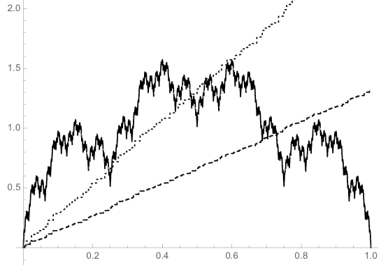
Figure 3: Plot of the function $\widehat{x}+y$ defined in (2.14). The dotted line is $\langle\widehat{x}+y\rangle^{7}$, the dashed line is $\langle\widehat{x}+y\rangle^{8}$.

3 Proofs

3.1 Proof of Theorem 2.2

We start with the following lemma, which computes maxima and maximizers of the functions

$$\widehat{x}^{n}(t):=\sum_{m=0}^{n-1}\sum_{k=0}^{2^{m}-1}e_{m,k}(t),\qquad t\in[0,1]\text{ and }n=1,2,\dots;$$

see Figure 4 for an illustration.

\begin{overpic}[width=341.43306pt]{graphics/Jacobsthal.pdf} \put(41.0,0.0){\scriptsize{$t_{2}$}} \put(51.0,0.0){\scriptsize{$t_{4}$}} \put(56.0,0.0){\scriptsize{$t_{5}$}} \put(61.0,0.0){\scriptsize{$t_{3}$}} \put(79.0,0.0){\scriptsize{$t_{1}=\frac{1}{2}$}} \put(-2.5,27.0){\scriptsize{$M_{1}$}} \put(-2.5,32.0){\scriptsize{$M_{2}$}} \put(-2.5,41.0){\scriptsize{$M_{3}$}} \put(-2.5,45.0){\scriptsize{$M_{4}$}} \put(-2.5,49.5){\scriptsize{$M_{5}$}} \put(98.0,16.2){\scriptsize{$n=1$}} \put(98.0,21.2){\scriptsize{$n=2$}} \put(98.0,26.2){\scriptsize{$n=3$}} \put(98.0,31.2){\scriptsize{$n=4$}} \put(98.0,36.2){\scriptsize{$n=5$}} \end{overpic}

Figure 4: Illustration of Lemma 3.1 and its proof. The functions ${\widehat{x}}^{n}$ are plotted over the interval $[0,1/2]$ for various values of $n$, together with the corresponding values for $t_{n}$ and $M_{n}$.

Lemma 3.1.

Let

$$J_{n}:=\frac{1}{3}(2^{n}-(-1)^{n})$$

be the sequence of Jacobsthal numbers, and let

$$M_{n}:=\frac{1}{3}\Big{(}2+\sqrt{2}+(-1)^{n+1}2^{-n}(\sqrt{2}-1)\Big{)}-2^{-n/2}.$$ (3.1)

The function ${\widehat{x}}^{n}$ has two maximal points given by

$$t_{n}^{-}:=2^{-n}J_{n}\in[0,1/2]\qquad\text{and}\qquad t_{n}^{+}:=1-t_{n}^{-}\in[1/2,1],$$ (3.2)

these are the only maximal points, and the global maximum of ${\widehat{x}}^{n}$ is given by

$$\max_{t\in[0,1]}{\widehat{x}}^{n}(t)={\widehat{x}}^{n}(t^{-}_{n})={\widehat{x}}^{n}(t^{+}_{n})=M_{n}.$$

Proof.

We first note that by the symmetry of ${\widehat{x}}^{n}$ with respect to $t=1/2$ and the fact that $t_{n}^{+}=1-t_{n}^{-}$ it is sufficient to prove the result for the restriction of ${\widehat{x}}^{n}$ to $[0,\frac{1}{2}]$. We will therefore simply write $t_{n}$ in place of $t_{n}^{-}$.

We will prove the assertion by induction on $n$. First, for $n=1$, we have ${\widehat{x}}^{n}(t)=e_{0,0}(t)=\min\{t,1-t\}$, which is maximized at $t=1/2=2^{-1}J_{1}$ and has the maximum $1/2=M_{1}$. Given that $t_{1}=1/2$, our claim that $t_{n}=2^{-n}J_{n}$ is now equivalent to the recursion

$$t_{n+1}=t_{n}+(-1)^{n}2^{-(n+1)}.$$ (3.3)

For $n=2$, the new maximum is taken at the peak of $e_{1,0}$, which is attained at $t=1/4=t_{1}-2^{-2}$. Hence (3.3) follows for $n=2$. Moreover,

$$\max_{t\in[0,1/2]}\widehat{x}^{2}(t)=\widehat{x}^{2}(1/4)=\frac{1}{4}+2^{-3/2}=M_{2}.$$

Clearly, the maximizers of $\widehat{x}^{1}$ and $\widehat{x}^{2}$ on $[0,1/2]$ are unique.

Now we assume that $n\geq 2$ and that the assertion has been established for $n$ and $n-1$. When letting

$$f_{m,k}:=e_{m,k}+e_{m+1,2k}+e_{m+1,2k+1},$$ (3.4)

the function $\widehat{x}^{n+1}$ can be obtained from

$$\widehat{x}^{n}=\widehat{x}^{n-1}+\sum_{k=0}^{2^{n-1}-1}e_{n-1,k}$$

by replacing all Faber–Schauder functions $e_{n-1,k}$ with the corresponding functions $f_{n-1,k}$, i.e.,

$$\widehat{x}^{n+1}=\widehat{x}^{n-1}+\sum_{k=0}^{2^{n-1}-1}f_{n-1,k}.$$

It follows from our induction hypothesis and the formula for $t_{n}$ that the maximum of $\widehat{x}^{n}$ is attained at the peak of some function $e_{n-1,k}$. Clearly, the support of $f_{n-1,k}$ coincides with the support of $e_{n-1,k}$, while the function $\widehat{x}^{n-1}$ is linear on that support. Moreover, the function $f_{n-1,k}$ has two maxima at $t_{n}-2^{-(n+1)}$ and $t_{n}+2^{-(n+1)}$, and these maxima are strictly bigger than the one of $e_{n-1,k}$; see Figure 5 for an illustration. It therefore follows that either $\widehat{x}^{n+1}(t_{n}+2^{-(n+1)})$ or $\widehat{x}^{n+1}(t_{n}-2^{-(n+1)})$ must be strictly larger than $\widehat{x}^{n}(t_{n})=\max_{t}\widehat{x}^{n}(t)$. Hence, the maximum of $\widehat{x}^{n+1}$ must be attained at the peak of some Faber–Schauder function $e_{n,\ell}$ for a certain $\ell\in\{0,\dots,2^{n}-1\}$. The support of $e_{n,\ell}$ is an interval with endpoints $s$ and $s^{\prime}$, and the peak of $e_{n,\ell}$ is located at $s^{*}=(s+s^{\prime})/2$ and has height $2^{-(n+2)/2}$. The function $\widehat{x}^{n}$, on the other hand, is linear on the support of $e_{n,\ell}$ so that the maximum of $\widehat{x}^{n+1}$ must satisfy

$$\max_{t\in[0,1/2]}\widehat{x}^{n+1}(t)=\widehat{x}^{n+1}(s^{*})=\widehat{x}^{n}(s^{*})+e_{n,\ell}(s^{*})=\frac{\widehat{x}^{n}(s)+\widehat{x}^{n}(s^{\prime})}{2}+2^{-\frac{n+2}{2}}.$$

At one of the endpoints of the interval enclosed by $s$ and $s^{\prime}$, say at $s^{\prime}$, the function $\widehat{x}^{n}$ coincides with $\widehat{x}^{n-1}$, and therefore the value $\widehat{x}^{n}(s^{\prime})$ can be estimated from above by $M_{n-1}$. The value $\widehat{x}^{n}(s)$, on the other hand, can be estimated from above by $M_{n}$. We hence arrive at

$$\widehat{x}^{n+1}(s^{*})\leq\frac{M_{n}+M_{n-1}}{2}+2^{-\frac{n+2}{2}}=M_{n+1}.$$ (3.5)

But we can achieve equality in (3.5) when taking for $s^{*}$ the midpoint between $t_{n}$ and $t_{n-1}$, which is possible since, inductively by (3.3), $t_{n}$ and $t_{n-1}$ enclose the interval of support of some Faber–Schauder function of generation $n$. When making this choice, we have moreover that

$$s^{*}=\frac{t_{n}+t_{n-1}}{2}=\frac{t_{n}+t_{n}-(-1)^{n-1}2^{-n}}{2}=t_{n+1}.$$

This proves that $\widehat{x}^{n+1}$ has maximum $M_{n+1}$ and is maximized at $t_{n+1}$. Moreover, $t_{n+1}$ is the unique maximizer of $\widehat{x}^{n+1}$ in $[0,1/2]$, since, by induction hypothesis, $s^{*}=(t_{n}+t_{n-1})/2$ is the only point at which equality can hold in (3.5). ∎

\begin{overpic}[width=256.0748pt]{graphics/fmk.pdf} \put(0.0,0.0){\scriptsize{$k2^{-m}$}} \put(16.0,0.0){\scriptsize{$(k+\frac{1}{4})2^{-m}$}} \put(37.0,0.0){\scriptsize{$(k+\frac{1}{2})2^{-m}$}} \put(57.0,0.0){\scriptsize{$(k+\frac{3}{4})2^{-m}$}} \put(77.0,0.0){\scriptsize{$(k+1)2^{-m}$}} \put(-9.5,42.0){\scriptsize{$2^{-\frac{m+2}{2}}$}} \put(-22.0,50.0){\scriptsize{$(1+\sqrt{2})2^{-\frac{m+4}{2}}$}} \put(98.0,24.5){\scriptsize{$e_{m,k}$}} \put(98.0,29.5){\scriptsize{$f_{m,k}$}} \end{overpic}

Figure 5: The function $f_{m,k}$ defined in (3.4), plotted alongside $e_{m,k}$.

Proof of Theorem 2.2. Part (a): For $t$ fixed, $x(t)=\sum_{m=0}^{\infty}\sum_{k=0}^{2^{m}-1}\theta_{m,k}e_{m,k}(t)$ is maximized by taking all coefficients $\theta_{m,k}$ equal to $+1$, i.e., $|x(t)|\leq|\widehat{x}(t)|$ for all $x\in{\mathscr{X}}$ and $t\in[0,1]$. The statement on maximum and maximizers of $\widehat{x}$ follows immediately from Lemma 3.1 by noting that $M_{n}\to\frac{1}{3}(2+\sqrt{2})$ and $t_{n}^{-}\to\frac{1}{3}$ as $n\uparrow\infty$.

Part (b): We first show that the maximal oscillation of an arbitrary $x\in{\mathscr{X}}$ is dominated by the maximal oscillation of $x^{*}$. See Figure 6 for a plot of $x^{*}$. To this end, we may assume without loss of generality that the coefficient $\theta_{0,0}$ in the Faber–Schauder development of $x$ is equal to $+1$. Next, we note that for $0\leq s\leq 1/2$,

$$x(s)\leq\widehat{x}(s)=x^{*}(s)$$ (3.6)

and

$$x(s)\geq e_{0,0}(s)-\big{(}\widehat{x}(s)-e_{0,0}(s)\big{)}=2e_{0,0}(1-s)-\widehat{x}(1-s)=x^{*}(1-s).$$ (3.7)

For $1/2\leq t\leq 1$, we get in the same manner that

$$x^{*}(t)\leq x(t)\leq x^{*}(1-t).$$ (3.8)

It follows that

$$\max_{s,t\in[0,1]}|x(t)-x(s)|\leq\max_{s\in[0,1/2]}\max_{t\in[1/2,1]}|x^{*}(t)-x^{*}(s)|,$$ (3.9)

and by taking $x=x^{*}$ we see that the right-hand side is in fact equal to $\max_{s,t\in[0,1]}|x^{*}(t)-x^{*}(s)|$.

To compute the right-hand side of (3.9), note that we have $x^{*}=\widehat{x}$ on $[0,1/2]$, and so the maximum of $x^{*}$ is attained in $s=1/3$ with value $\frac{1}{3}(2+\sqrt{2})$, due to the first part of this theorem. Moreover, on $[1/2,1]$ we have that $-x^{*}(t)=\widehat{x}({t-1/2})-1/2$. It therefore follows from part (a) of the theorem that the minimum of $x^{*}$ is attained at $t=5/6$ with minimal value $\frac{1}{2}-\frac{1}{3}(2+\sqrt{2})$; see Figure 6. Therefore,

$$\max_{s\in[0,1/2]}\max_{t\in[1/2,1]}|x^{*}(t)-x^{*}(s)|=\frac{2}{3}(2+\sqrt{2})-\frac{1}{2}=\frac{5}{6}+\frac{\sqrt{8}}{3}.$$ ∎

\begin{overpic}[width=256.0748pt]{graphics/x_star.pdf} \put(0.0,21.0){\scriptsize{$0$}} \put(31.6,21.0){\scriptsize{$1/3$}} \put(47.0,21.0){\scriptsize{$1/2$}} \put(79.0,21.0){\scriptsize{$5/6$}} \put(-20.0,2.5){\scriptsize{$\frac{1}{2}-\frac{1}{3}(2+\sqrt{2})$}} \put(-0.5,39.5){\scriptsize{$\frac{1}{2}$}} \put(-13.5,59.5){\scriptsize{$\frac{1}{3}(2+\sqrt{2})$}} \end{overpic}

Figure 6: The function $x^{*}$ with its maximum and minimum, and the function $e_{0,0}$ (dashed).

3.2 Proofs of Theorem 2.3 and of Corollary 2.5

Let $h>0$ be given, and define $n:=\nu(h)$ so that $2^{-(n+1)}<h\leq 2^{-n}$. Faber–Schauder functions $e_{m,k}$ can be linear with slope $\pm 2^{m/2}$ on intervals of length $2^{-(m+1)}$. Using this fact for $m\leq n-2$ and for the interval $[t,t+2^{-n}]$, we get

$$|x(t+h)-x(t)| \leq\sum_{m=0}^{n-2}h2^{m/2}+\bigg{|}\sum_{m=n-1}^{\infty}\sum_{k=0}^{2^{m}-1}\theta_{m,k}\Big{(}e_{m,k}(t+h)-e_{m,k}(t)\Big{)}\bigg{|},$$ (3.10)

where $\theta_{m,k}$ are the coefficients in the Faber–Schauder development of $x$. The left-hand sum is equal to $h(1+\sqrt{2})(2^{(n-1)/2}-1)$. This observation suffices in the situation of [20] and [1] to determine the corresponding moduli of continuity, because in these papers the Faber–Schauder coefficients are such that the sum on the right-hand side can be asymptotically neglected.

In our case, the sum on the right-hand side of (3.10) will turn out to be of the same order as $h2^{\nu(h)}$ and therefore cannot be neglected. To deal with it, we note that the Faber–Schauder functions have the following scaling properties:

$$\sqrt{2}e_{m,k}(t)=e_{{m-1},k}(2t)\qquad\text{and}\qquad e_{m,k}(t-\ell 2^{-m})=e_{m,k+\ell}(t)$$ (3.11)

for $t\in{\mathbb{R}}$, $m\geq 0$, and $k,\ell\in\mathbb{Z}$. For $t\in[0,1-2^{-n})$ given, let $\ell\in\mathbb{N}_{0}$ be such that $\ell 2^{-n}\leq t<(\ell+1)2^{-n}$ and define $s:=t-\ell 2^{-n}$. Then $0\leq 2^{n-1}s<1/2$ and $1/4<2^{n-1}(s+h)<1$. The scaling properties (3.11) imply that for $m\geq n$,

$$e_{m,k}(t+h)-e_{m,k}(t)=2^{\frac{1-n}{2}}\big{(}e_{m-(n-1),k-\ell 2^{m-n}}(2^{n-1}(s+h))-e_{m-(n-1),k-\ell 2^{m-n}}(2^{n-1}s)\big{)}.$$ (3.12)

The case $m=n-1$ needs additional care, depending on whether $\ell$ is even or odd.

Case 1: $\ell$ is even. In this case, $[\ell 2^{-n},(\ell+2)2^{-n}]$ contains both $t$ and $t+h$ and is equal to the support of $e_{n-1,\ell/2}$. Therefore, the identity (3.12) extends to $m=n-1$ and we arrive at

$$\sum_{m=n-1}^{\infty}\sum_{k=0}^{2^{m}-1}\theta_{m,k}\Big{(}e_{m,k}(t+h)-e_{m,k}(t)\Big{)}=2^{\frac{1-n}{2}}\big{(}y(2^{n-1}(s+h)))-y(2^{n-1}s)\big{)}$$ (3.13)

for

$$y:=\sum_{m=0}^{\infty}\sum_{k=0}^{2^{m}-1}\theta_{m+n-1,k+\ell 2^{m-1}}e_{m,k}\in{\mathscr{X}}.$$ (3.14)

Case 2: $\ell$ is odd. In this case, the interval $[\ell 2^{-n},(\ell+1)2^{-n}]$ contains $t$ and belongs to the support of $e_{n-1,(\ell-1)/2}$, while the interval $[(\ell+1)2^{-n},(\ell+2)2^{-n}]$ belongs to the support of $e_{n-1,(\ell+1)/2}$. The point $t+h$ may belong to either of the two intervals. We need to distinguish two further cases, depending on whether the coefficients $\theta_{n-1,(\ell-1)/2}$ and $\theta_{n-1,(\ell+1)/2}$ are identical or different.

Case 2a: $\theta_{n-1,(\ell-1)/2}=\theta_{n-1,(\ell+1)/2}$. We have

$$e_{n-1,(\ell-1)/2}(r)+e_{n-1,(\ell+1)/2}(r)=2^{\frac{1-n}{2}}\Big{(}\frac{1}{2}-e_{0,0}(2^{{n-1}}r-\ell/2)\Big{)}\qquad\text{for $r\in[\ell 2^{-n},(\ell+2)2^{-n}]$.}$$

We thus arrive again at (3.13), but this time for

$$y:=-\theta_{n-1,(\ell-1)/2}e_{0,0}+\sum_{m=1}^{\infty}\sum_{k=0}^{2^{m}-1}\theta_{m+n-1,k+\ell 2^{m-1}}e_{m,k}\in{\mathscr{X}}.$$

Case 2b: $\theta_{n-1,(\ell-1)/2}=-\theta_{n-1,(\ell+1)/2}$. Since $e_{n-1,(\ell-1)/2}(r)-e_{n-1,(\ell+1)/2}(r)$ is linear on $[\ell 2^{-n},(\ell+2)2^{-n}]$ with slope $-2^{\frac{n-1}{2}}$, we get

$$\begin{split}|x(t+h)-x(t)|&\leq\sum_{m=0}^{n-1}h2^{m/2}+\bigg{|}\sum_{m=n}^{\infty}\sum_{k=0}^{2^{m}-1}\theta_{m,k}\Big{(}e_{m,k}(t+h)-e_{m,k}(t)\Big{)}\bigg{|}\\ &=h(1+\sqrt{2})(2^{n/2}-1)+2^{-n/2}|y(2^{n}(s+h)))-y(2^{n}s)|,\end{split}$$ (3.15)

where

$$y(r)=\begin{cases}y_{0}(r)&\text{if $0\leq r\leq 1$,}\\ y_{1}(r-1)&\text{if $1\leq r\leq 2$,}\end{cases}$$ (3.16)

and $y_{0},y_{1}\in{\mathscr{X}}$ are given by

$$y_{0}:=\sum_{m=0}^{\infty}\sum_{k=0}^{2^{m}-1}\theta_{m+n,k+\ell 2^{m}}e_{m,k},\qquad y_{1}:=\sum_{m=0}^{\infty}\sum_{k=0}^{2^{m}-1}\theta_{m+n,k+(\ell+1)2^{m}}e_{m,k}$$ (3.17)

See Figure 7 for an illustration in which $y_{0}=\widehat{x}=-y_{1}$, as it will be needed in the proof of Theorem 2.3 (b).

Proof of Theorem 2.3 (a).

Let again $h>0$ be given with $n=\nu(h)$. Since $\theta_{m,k}=1$ for all $m,k$, (3.10), (3.13), (3.14), and Theorem 2.2 (a) imply that in Case 1

$$|\widehat{x}(t+h)-\widehat{x}(t)| \leq h(1+\sqrt{2})(2^{(n-1)/2}-1)+2^{\frac{1-n}{2}}\big{|}\widehat{x}(2^{n-1}(s+h)))-\widehat{x}(2^{n-1}s)\big{|}$$ (3.18)

$$\leq h(1+\sqrt{2})2^{(n-1)/2}+\frac{2^{\frac{1-n}{2}}}{3}(2+\sqrt{2})=\omega(h).$$

In Case 2a we get a similar estimate, but on the right-hand side of (3.18), $\widehat{x}$ needs to be replaced by

$$\widehat{y}:=-e_{0,0}+\sum_{m=1}^{\infty}\sum_{k=0}^{2^{m}-1}e_{m,k}.$$

But note that $\widehat{y}(t)=\widehat{x}(\varphi(t))-1/2$, where $\varphi(t)=1/2-t$ for $t\leq 1/2$ and $\varphi(t)=t-1/2$ for $t\geq 1/2$. Therefore, $|\widehat{x}(t+h)-\widehat{x}(t)|\leq\omega(h)$ also holds in Case 2a. Finally, Case 2b cannot occur. This concludes the proof of “$\leq$”.

To prove “$\geq$”, we let $t:=0$ and $h_{n}:=\frac{2}{3}2^{-n}$. Then we are in Case 1, and

$$|\widehat{x}(t+h_{n})-\widehat{x}(t)|=(1+\sqrt{2})(2^{(n-1)/2}-1)h_{n}+2^{(1-n)/2}\widehat{x}(2^{n-1}h_{n})=\omega(h_{n})-(1+\sqrt{2})h_{n},$$

by Theorem 2.2 (a). Since $\omega(h_{n})=O(\sqrt{h_{n}})$, we get “$\geq$”.∎

Proof of Theorem 2.3 (b).

Let again $h>0$ be given with $n=\nu(h)$. In Case 1, (3.10), (3.13), (3.14), and Theorem 2.2 (b) imply that for each $x\in{\mathscr{X}}$

$$|x(t+h)-x(t)| \leq h(1+\sqrt{2})(2^{(n-1)/2}-1)+2^{\frac{1-n}{2}}\sup_{y\in{\mathscr{X}}}\big{|}y(2^{n-1}(s+h)))-y(2^{n-1}s)\big{|}$$

$$\leq h(1+\sqrt{2})2^{(n-1)/2}+\frac{2^{\frac{1-n}{2}}}{6}(5+4{\sqrt{2}})$$

$$=(1+\sqrt{2})h2^{n/2}-\frac{2^{\log_{2}h+n/2}}{\sqrt{2}}+\frac{1}{3}\Big{(}\frac{5}{\sqrt{2}}+4\Big{)}2^{-n/2}.$$ (3.19)

Since $\log_{2}h+n/2\geq-n/2-1$, the middle term of the preceding sum is bounded from above by $-2^{-n/2}/\sqrt{8}$, and so the entire sum in (3.19) is dominated by

$$(1+\sqrt{2})h2^{n/2}+\frac{1}{3}\Big{(}\frac{5}{\sqrt{2}}+4-\frac{3}{\sqrt{8}}\Big{)}2^{-n/2},$$

which is in turn dominated by $\sqrt{2}\omega(h)$.

The same inequality as in Case 1 holds in Case 2a. In Case 2b, we obtain

$$|x(t+h)-x(t)| \leq h(1+\sqrt{2})(2^{n/2}-1)+2^{-n/2}\sup_{0\leq r\leq 2}\sup_{0\leq s\leq 2}|y(r)-y(s)|,$$

where $y$ is as in (3.16) for $y_{0},y_{1}\in{\mathscr{X}}$. Clearly, the supremum on the right-hand side is maximized when $y_{0}=-y_{1}=\widehat{x}$ and then equal to $\frac{2}{3}(2+\sqrt{2})$ according to Theorem 2.2 (a). Therefore,

$$|x(t+h)-x(t)|\leq h(1+\sqrt{2})2^{n/2}+2^{-n/2}\frac{2}{3}(2+\sqrt{2})=\sqrt{2}\omega(h).$$

This concludes the proof of “$\leq$”.

To prove “$\geq$”, we let

$$t_{n}:=\frac{1}{2}-\frac{1}{3}2^{-n}\qquad\text{and}\qquad h_{n}:=\frac{2}{3}2^{-n},$$

so that $\nu(h_{n})=n$. When considering the function $x_{*}:=-x^{*}\in{\mathscr{X}}$, we are in Case 2b. First, we have $e_{0,0}(t_{n}+h_{n})-e_{0,0}(t_{n})=0$. Second, for $m=1,\dots,n$, the function

$$g_{m}:=-e_{m,2^{m-1}-1}+e_{m,2^{m-1}}$$

is linear on $[\frac{1}{2}-2^{-m-1},\frac{1}{2}+2^{-m-1}]\supset[t_{n},t_{n}+h_{n}]$ with slope $2^{m/2}$. Using this fact for $m\leq n-1$ gives

$$x_{*}(t_{n}+h_{n})-x_{*}(t_{n}) =\sum_{m=1}^{n-1}2^{m/2}h_{n}+\sum_{m=n}^{\infty}\bigg{(}\sum_{\ell=2^{m-1}}^{2^{m}-1}e_{m,\ell}(t_{n}+h_{n})+\sum_{k=0}^{2^{m-1}-1}e_{m,k}(t_{n})\bigg{)}$$

$$=(1+\sqrt{2})(2^{n/2}-\sqrt{2})h_{n}+2^{-n/2}\big{(}\widehat{x}(1/3)+\widehat{x}(2/3)\big{)}$$

$$=(1+\sqrt{2})2^{n/2}h_{n}-(\sqrt{2}+2)h_{n}+2^{-n/2}\frac{2}{3}(2+\sqrt{2})$$

$$=\sqrt{2}\omega(h_{n})-(\sqrt{2}+2)h_{n},$$

where, in the second step, we have argued as in (3.15), and, in the third step, we have used Theorem 2.2 (a); see Figure 7 for an illustration. Since $\omega(h_{n})=O(\sqrt{h_{n}})$, we get “$\geq$”. ∎

\begin{overpic}[width=426.79134pt]{graphics/xlowerstar.pdf} \put(20.0,21.0){\scriptsize{$2^{-(n-1)}$}} \put(38.0,21.0){\scriptsize{$t_{n}$}} \put(44.3,17.5){\scriptsize{$t_{n}+h_{n}$}} \put(59.0,17.5){\scriptsize{$\frac{1}{2}+2^{-(n-1)}$}} \put(82.2,17.5){\scriptsize{$1$}} \put(98.0,9.7){\scriptsize{$m\geq 3$}} \put(98.0,14.7){\scriptsize{$m=2$}} \put(98.0,19.7){\scriptsize{$m=1$}} \put(98.0,24.7){\scriptsize{$m=0$}} \end{overpic}

Figure 7: Illustration of Case 2b and, in particular, of the proof of ‘$\geq$’ in Theorem 2.3 (b) for $n=3$. The functions $e_{m,k}$ in the Faber–Schauder development of $x_{*}=-x^{*}$ are plotted individually for generations $m\leq n-1$. Their sum over all generations $m\geq n$ corresponds to a sequence of rescaled functions $\widehat{x}$.

Proof of Corollary 2.5.

Theorem 2.2 implies that the family ${\mathscr{X}}$ is uniformly bounded and Theorem 2.3 (b) yields that ${\mathscr{X}}$ is equicontinuous. Therefore it only remains to show that ${\mathscr{X}}$ is closed in $C[0,1]$. Following Hata and Yamaguti [20], let $(x_{n})_{n\in\mathbb{N}}$ be a sequence in ${\mathscr{X}}$ that converges uniformly to some $x\in C[0,1]$. We clearly have $x(0)=x(1)=0$. It is well known that any such function can be uniquely represented as a uniformly convergent series of Faber–Schauder functions,

$$x=\sum_{m=0}^{\infty}\sum_{k=0}^{2^{m}-1}a_{m,k}(x)e_{m,k},$$ (3.20)

where the coefficients $a_{m,k}$ are given as

$$a_{m,k}(x)=2^{m/2}\bigg{(}2x\Big{(}\frac{2k+1}{2^{m+1}}\Big{)}-x\Big{(}\frac{k}{2^{m}}\Big{)}-x\Big{(}\frac{k+1}{2^{m}}\Big{)}\bigg{)}.$$

Clearly, we have $a_{m,k}(x_{n})\to a_{m,k}(x)$ for all pairs $m,k$ as $n\uparrow\infty$. But since each $x_{n}\in{\mathscr{X}}$ and the representation (3.20) is unique, we must have $a_{m,k}(x_{m})\in\{-1,+1\}$, which implies that also $a_{m,k}(x)\in\{-1,+1\}$ and in turn that $x\in{\mathscr{X}}$. ∎

3.3 Proofs of Propositions 2.6 and 2.7

Remark 3.2.

As already observed in [26, Remark 8], the following facts follow easily from Propositions 2.2.2, 2.2.9, and 2.3.2 in [28]. Suppose that $x\in C[0,1]$ admits the continuous quadratic variation $\langle x\rangle$ along $(\mathbb{T}_{n})$ and $f$ is continuous and of finite variation. Then both $\langle f\rangle$ and $\langle x+f\rangle$ exist along $(\mathbb{T}_{n})$ and are given by $\langle f\rangle=0$ and $\langle x+f\rangle=\langle x\rangle$. By means of the polarization identity (2.10) we get moreover that $\langle x,f\rangle=0$.

Proof of Proposition 2.6.

Lemma 1.1 (ii) in [19] states that a function $x\in C[0,1]$ with Faber–Schauder development $\sum_{m=0}^{\infty}\sum_{k=0}^{2^{m}-1}\theta_{m,k}e_{m,k}$ satisfies

$$\langle x\rangle_{1}^{n}=\frac{1}{2^{n}}\sum_{m=0}^{n-1}\sum_{k=0}^{2^{m}-1}\theta_{m,k}^{2}.$$

This immediately yields $\langle x\rangle_{1}=1$ for all $x\in{\mathscr{X}}$.

The first scaling property in (3.11) implies that for any $x\in{\mathscr{X}}$ there exists $y\in{\mathscr{X}}$ and a linear function $f$ such that $x(t)=f(2t)+2^{-1/2}y(2t)$ for $0\leq t\leq 1/2$. It hence follows from Remark 3.2 that $\langle x\rangle_{\frac{1}{2}}=\langle f+2^{-1/2}y\rangle_{1}=\langle 2^{-1/2}y\rangle_{1}=1/2$. Iteratively, we obtain $\langle x\rangle_{2^{-\ell}}=2^{-\ell}$ for all $\ell\in\mathbb{N}$. Using also the second scaling property in (3.11) gives in a similar manner that $\langle x\rangle_{(k+1)2^{-\ell}}-\langle x\rangle_{k2^{-\ell}}=2^{-\ell}$ for $k,\ell\in\mathbb{N}$ with $(k+1)2^{-\ell}\leq 1$. We therefore arrive at $\langle x\rangle_{t}=t$ for all dyadic rationals $t\in[0,1]$. A sandwich argument extends this fact to all $t\in[0,1]$.∎

For $x\in{\mathscr{X}}$ with Faber–Schauder expansion $x=\sum_{m=0}^{\infty}\sum_{k=0}^{2^{m}-1}\theta_{m,k}e_{m,k}$ and $n\in\mathbb{N}$, we define $x^{n}$ by (2.1).

Proof of Proposition 2.7.

We first show (2.13) for $t=1$. To this end, we note that $x(s)=x^{n+k}(s)$ for $s\in\mathbb{T}_{n}$ and $k\geq 0$. Hence,

$$\langle\widehat{x},y\rangle^{n}_{1}:=\sum_{s\in\mathbb{T}_{n}}(\widehat{x}(s^{\prime})-\widehat{x}(s))(y(s^{\prime})-y(s))=\sum_{s\in\mathbb{T}_{n}}(\widehat{x}^{n}(s^{\prime})-\widehat{x}^{n}(s))(y^{n}(s^{\prime})-y^{n}(s)).$$ (3.21)

Moreover,

$$\widehat{x}^{n+1}\Big{(}\frac{s+s^{\prime}}{2}\Big{)}=\widehat{x}^{n}\Big{(}\frac{s+s^{\prime}}{2}\Big{)}+\Delta_{n+1}=\frac{1}{2}(\widehat{x}^{n}(s)+\widehat{x}^{n}(s^{\prime}))+\Delta_{n+1},$$

where $\Delta_{n+1}=2^{-(n+2)/2}$ is the maximal amplitude of a Faber–Schauder function $e_{n,\ell}$. Similarly, for $y$ we have

$$y^{n+1}\Big{(}\frac{s+s^{\prime}}{2}\Big{)}=y^{n}\Big{(}\frac{s+s^{\prime}}{2}\Big{)}+(-1)^{n+1}\Delta_{n+1}=\frac{1}{2}(y^{n}(s)+y^{n}(s^{\prime}))+(-1)^{n+1}\Delta_{n+1}.$$

Therefore, when passing from $n$ to $n+1$ in (3.21), each term $(\widehat{x}^{n}(s^{\prime})-\widehat{x}^{n}(s))(y^{n}(s^{\prime})-y^{n}(s))$ will be replaced by

$$\Big{(}\widehat{x}^{n+1}(s^{\prime})- \widehat{x}^{n+1}\Big{(}\frac{s+s^{\prime}}{2}\Big{)}\Big{)}\Big{(}y^{n+1}(s^{\prime})-y^{n+1}\Big{(}\frac{s+s^{\prime}}{2}\Big{)}\Big{)}$$

$$+\Big{(}\widehat{x}^{n+1}\Big{(} \frac{s+s^{\prime}}{2}\Big{)}-\widehat{x}^{n+1}(s)\Big{)}\Big{(}y^{n+1}\Big{(}\frac{s+s^{\prime}}{2}\Big{)}-y^{n+1}(s)\Big{)}$$

$$=\Big{(}\frac{1}{2}\big{(}\widehat{x}^{n}(s^{\prime})-\widehat{x}^{n}(s)\big{)}-\Delta_{n+1}\Big{)}\Big{(}\frac{1}{2}\big{(}y^{n}(s^{\prime})-y^{n}(s)\big{)}-(-1)^{n+1}\Delta_{n+1}\Big{)}$$

$$\qquad+\Big{(}\frac{1}{2}\big{(}\widehat{x}^{n}(s^{\prime})-\widehat{x}^{n}(s)\big{)}+\Delta_{n+1}\Big{)}\Big{(}\frac{1}{2}\big{(}y^{n}(s^{\prime})-y^{n}(s)\big{)}+(-1)^{n+1}\Delta_{n+1}\Big{)}$$

$$=\frac{1}{2}(\widehat{x}^{n}(s^{\prime})-\widehat{x}^{n}(s))(y^{n}(s^{\prime})-y^{n}(s))+2(-1)^{n+1}\Delta_{n+1}^{2}$$

$$=\frac{1}{2}(\widehat{x}^{n}(s^{\prime})-\widehat{x}^{n}(s))(y^{n}(s^{\prime})-y^{n}(s))+(-1)^{n+1}2^{-n-1}$$

So

$$\langle\widehat{x},y\rangle^{n+1}_{1}=\frac{1}{2}\langle\widehat{x},y\rangle^{n}_{1}+(-1)^{n+1}\sum_{s\in\mathbb{T}_{n}}2^{-n-1}=\frac{1}{2}\Big{(}\langle\widehat{x},y\rangle^{n}_{1}+(-1)^{n+1}\Big{)}$$

and in turn

$$\langle\widehat{x},y\rangle^{2n+1}_{1}=\frac{1}{4}\langle\widehat{x},y\rangle^{2n-1}_{1}+\frac{1}{4}\qquad\text{and}\qquad\langle\widehat{x},y\rangle^{2n+2}_{1}=\frac{1}{4}\langle\widehat{x},y\rangle^{2n}_{1}-\frac{1}{4}.$$

This recursion easily implies (2.13) for $t=1$.

Next, still for $t=1$, the identities (2.12) follow immediately from (2.13) and the polarization identity (2.10). To prove (2.12) for all $t\in[0,1]$, we note that the Faber–Schauder expansion (2.14) of $\widehat{y}:=\widehat{x}+y$ and the first scaling property in (3.11) imply the following self-similarity relation: $\widehat{y}(t)=f(4t)+\frac{1}{2}\widehat{y}(4t)$, where $0\leq t\leq 1/4$ and $f$ is a piecewise linear function and hence of bounded variation. It therefore follows as in the proof of Proposition 2.6 that, if the quadratic variation $\langle\widehat{y}\rangle_{1}$ exists along some subsequence of $(\mathbb{T}_{n})$, then $\langle\widehat{y}\rangle_{\frac{1}{4}}$ also exists along that subsequence and equals $\frac{1}{4}\langle\widehat{y}\rangle_{1}$. The two identities (2.12) now follow as in the proof of Proposition 2.6 and by further exploiting the self-similarity of $\widehat{y}$. By using once again polarization (2.10), we finally arrive at (2.13) for all $t\in[0,1]$. ∎

Acknowledgement. The author expresses his gratitude toward two anonymous referees for valuable comments and suggestions that helped to improve the paper substantially.

References

• [1] P. C. Allaart. On a flexible class of continuous functions with uniform local structure. Journal of the Mathematical Society of Japan, 61(1):237–262, 2009.
• [2] P. C. Allaart and K. Kawamura. The Takagi function: a survey. Real Analysis Exchange, 37(1):1–54, 2011.
• [3] C. Bender, T. Sottinen, and E. Valkeila. Pricing by hedging and no-arbitrage beyond semimartingales. Finance Stoch., 12(4):441–468, 2008.
• [4] A. Bick and W. Willinger. Dynamic spanning without probabilities. Stochastic Process. Appl., 50(2):349–374, 1994.
• [5] P. Billingsley. Van der Waerden’s continuous nowhere differentiable function. Am. Math. Mon., 89:691, 1982.
• [6] R. Cont and D.-A. Fournié. Change of variable formulas for non-anticipative functionals on path space. J. Funct. Anal., 259(4):1043–1072, 2010.
• [7] R. Cont and D.-A. Fournié. Functional Itô calculus and stochastic integral representation of martingales. Ann. Probab., 41(1):109–133, 2013.
• [8] M. Davis, J. Obłój, and V. Raval. Arbitrage bounds for prices of weighted variance swaps. To appear in Mathematical Finance, 2014.
• [9] G. de Rham. Sur un exemple de fonction continue sans dérivée. Enseign. Math, 3:71–72, 1957.
• [10] B. Dupire. Functional Itô calculus. Bloomberg Portfolio Research Paper No. 2009-04-FRONTIERS, 2009. Available at http://dx.doi.org/10.2139/ssrn.1435551.
• [11] I. Ekren, C. Keller, N. Touzi, and J. Zhang. On viscosity solutions of path dependent PDEs. Ann. Probab., 42(1):204–236, 2014.
• [12] G. Faber. Über die Orthogonalfunktionen des Herrn Haar. Jahresbericht der deutschen Mathematiker-Vereinigung, 19:104–112, 1910.
• [13] H. Föllmer. Calcul d’Itô sans probabilités. In Seminar on Probability, XV (Univ. Strasbourg, Strasbourg, 1979/1980), volume 850 of Lecture Notes in Math., pages 143–150. Springer, Berlin, 1981.
• [14] H. Föllmer. Probabilistic aspects of financial risk. In European Congress of Mathematics, Vol. I (Barcelona, 2000), volume 201 of Progr. Math., pages 21–36. Birkhäuser, Basel, 2001.
• [15] H. Föllmer and A. Schied. Probabilistic aspects of finance. Bernoulli, 19(4):1306–1326, 2013.
• [16] D. Freedman. Brownian motion and diffusion. Springer-Verlag, New York, second edition, 1983.
• [17] P. K. Friz and M. Hairer. A course on rough paths. Springer-Verlag, Heidelberg, 2014.
• [18] N. Gantert. Einige grosse Abweichungen der Brownschen Bewegung. Dissertation, Rheinische Friedrich-Wilhelms-Universität Bonn; Bonner Mathematische Schriften, 224. 1991.
• [19] N. Gantert. Self-similarity of Brownian motion and a large deviation principle for random fields on a binary tree. Probab. Theory Related Fields, 98(1):7–20, 1994.
• [20] M. Hata and M. Yamaguti. The Takagi function and its generalization. Japan J. Appl. Math., 1(1):183–199, 1984.
• [21] J.-P. Kahane. Sur l’exemple, donné par M. de Rham, d’une fonction continue sans dérivée. Enseignement Math, 5:53–57, 1959.
• [22] I. Karatzas and S. E. Shreve. Brownian motion and stochastic calculus, volume 113 of Graduate Texts in Mathematics. Springer-Verlag, New York, second edition, 1991.
• [23] N. Kôno. On generalized Takagi functions. Acta Math. Hungar., 49(3-4):315–324, 1987.
• [24] J. C. Lagarias. The Takagi function and its properties. In Functions in number theory and their probabilistic aspects, RIMS Kôkyûroku Bessatsu, B34, pages 153–189. Res. Inst. Math. Sci. (RIMS), Kyoto, 2012.
• [25] F. Ledrappier. On the dimension of some graphs. In Symbolic dynamics and its applications (New Haven, CT, 1991), volume 135 of Contemp. Math., pages 285–293. Amer. Math. Soc., Providence, RI, 1992.
• [26] A. Schied. Model-free CPPI. J. Econom. Dynam. Control, 40:84–94, 2014.
• [27] A. Schied and M. Stadje. Robustness of delta hedging for path-dependent options in local volatility models. J. Appl. Probab., 44(4):865–879, 2007.
• [28] D. Sondermann. Introduction to stochastic calculus for finance, volume 579 of Lecture Notes in Economics and Mathematical Systems. Springer-Verlag, Berlin, 2006.
• [29] T. Takagi. A simple example of the continuous function without derivative. In Proc. Phys. Math. Soc. Japan, volume 1, pages 176–177, 1903.