Two-time distribution functions in the Gaussian model of randomly forced Burgers turbulence

Abstract

The problem of randomly forced Burgers turbulence is considered in terms of the toy Gaussian Larkin model of directed polymers. In terms of the replica technique the explicit expressions for the two-time four-point free energy distribution function is obtained which makes possible to derive the exact result for the two-time velocity distribution function in the corresponding Burgulence problem.

I Introduction

The KPZ problem KPZ describing the growth in time of an interface in the presence of noise have been the subject of intense investigations during the past almost three decades hh_zhang_95 ; burgers_74 ; kardar_book ; hhf_85 ; numer1 ; numer2 ; kardar_87 ; bouchaud-orland ; Brunet-Derrida ; Johansson ; Prahofer-Spohn ; Ferrari-Spohn1 . During last five years the major progress in solving this problem has been achieved which resulted in derivation of the exact solutions for various types of the free energy probability distribution function (PDF) KPZ-TW1a ; KPZ-TW1b ; KPZ-TW1c ; KPZ-TW2 ; BA-TW1 ; BA-TW2 ; BA-TW3 ; LeDoussal1 ; LeDoussal2 ; end-point ; goe ; LeDoussal3 ; Corwin ; Borodin ; Prolhac-Spohn ; 2pointPDF ; Imamura-Sasamoto-Spohn ; Prolhac-Spohn-N ; 2time ; Npoint .

In this paper I would like to consider the possibility to apply the ideas and technique developed in the studies of the KPZ problem for formally equivalent problem of the randomly forced Burgers turbulence (the ”Burgulence” problem). Here one considers a velocity field $v(x,t)$ governed by the Burgers equation

$$\partial_{t}v(x,t)+v(x,t)\partial_{x}v(x,t)=\nu\partial^{2}_{x}v(x,t)+\zeta(x,t)$$ (1)

where the parameter $\nu$ is the viscosity and $\zeta(x,t)$ is the Gaussian distributed random force which is $\delta$-correlated in time and which is characterized by finite correlation length $\xi$ in space: $\overline{\zeta(x,t)\zeta(x^{\prime},t^{\prime})}=u\delta(t-t^{\prime})U[(x-x^{\prime})/\xi]$. Here U(x) is a smooth function decaying to zero fast enough at large arguments and the parameter $u$ is the injected energy density. In this problem one would like to derive e.g. the the probability distribution functions of the velocity gradients $P[\partial_{x}v(x,t)]$ or two-points distribution function $P[v(x,t),v(x^{\prime},t)]$ at scales smaller than the length scale $\xi$ of the stirring force $\zeta$ (see e.g. burgers_74 ; Sinai ; Bouch-Mez-Par ; burgulence and references there in).

Formally the above problem is equivalent to the KPZ equation as well as to the (1+1) directed polymers. Indeed, redefining $v(x,t)=-\partial_{x}F(x,t)$ and $\zeta(x,t)=-\partial_{x}V(x,t)$ one gets the KPZ equation for the interface profile $F(x,t)$ (which is the free energy of (1+1) directed polymers):

$$\partial_{t}F(x,t)=\frac{1}{2}\bigl{(}\partial_{x}F(x,t)\bigr{)}^{2}-\frac{1}{2}T\partial^{2}_{x}F(x,t)-V(x,t)$$ (2)

where $T=2\nu$ is the temperature parameter of the directed polymer problem and $V(x,t)$ is the Gaussian distributed random potential.

The idea of a new approach to the Burgulence problem which I would like to demonstrate in this paper is in the following. According to the above definitions the velocity field can be represented as

$$v(x,t)=\lim_{\epsilon\to 0}[F(x+\epsilon,t)-F(x,t)]/\epsilon$$ (3)

Thus, deriving the four-point KPZ probability distribution function ${\cal P}[F(x+\epsilon,t),F(x,t),F(x^{\prime}+\epsilon,t^{\prime}),F(x^{\prime},t^{\prime})]$ and taking the limit $\epsilon\to 0$ one could hopefully obtain the result for $P[v(x,t),v(x^{\prime},t^{\prime})]$. The only ”little problem” is that unlike the usual KPZ studies operating with the $\delta$-correlated in space random potential, in the Burgulence problem one is mainly interested in the spatial scales comparable or much smaller than the random potential correlation length $\xi$. In other words, in this approach, first one has to study KPZ problem with random potentials having finite correlation length. In the present study (as a matter of ”warming up” exercise) I’m going to consider another ”extreme case” in which the random potential $V(x,t)$ of the KPZ problem is changed by it’s linear approximation: $V(x,t)\to\zeta(t)x$ where $\zeta(t)$ is Gaussian distributed random force. In this case we obtain the model introduced by Larkin Larkin ; Larkin-Ovchinnikov long time ago to study small scale displacements of directed polymers. In this approximation the model becomes Gaussian and therefore exactly solvable. Nevertheless, the statistical properties of its free energy (as well as some others quantities) turn out to be rather non-trivial (see e.g Gorochov-Blatter ; gaussian ; replicas ). For that reason this model hopefully could serve as a good ground for testing various approaches developed in the recent KPZ studies.

In Section II we introduce the model and formulate the main ideas of the replica approach which will be used in the further calculations of the two-time free energy distribution functions (for the directed polymer model) and the corresponding velocity distribution function (in the Burgulence problem). In Section III as the matter of the demonstration of the replica technique the explicit expression for the two-time (two-point) free energy distribution function is derived. In Section IV the two-time four-point free energy distribution function is calculated and the corresponding two-time velocity distribution function $P[v(x,t),v(x^{\prime},t^{\prime})]$ of the Burgulence problem is obtained. Further perspectives of the present approach is discussed in Section V.

II The model and the method

In this paper we consider the model of one-dimensional directed polymers defined in terms of an elastic string $\phi(\tau)$ directed along the $\tau$-axes within an interval $[0,t]$ which passes through a random medium described by a random potential $V(\phi,\tau)\;=\;\zeta(\tau)\phi$. The energy of a given polymer’s trajectory $\phi(\tau)$ is given by the Hamiltonian

$$H[\phi(\tau),V]=\int_{0}^{t}d\tau\Bigl{\{}\frac{1}{2}\bigl{[}\partial_{\tau}\phi(\tau)\bigr{]}^{2}+\zeta(\tau)\phi(\tau)\Bigr{\}};$$ (4)

where the random force $\zeta(\tau)$ is described by the Gaussian distribution with a zero mean $\overline{\zeta(\tau)}=0$ and the $\delta$-correlations:

$${\overline{\zeta(\tau)\zeta(\tau^{\prime})}}=u\delta(\tau-\tau^{\prime})$$ (5)

The parameter $u$ describes the strength of the disorder.

For the fixed boundary conditions, $\phi(0)=y;\;\phi(t)=x$, the partition function of the model (4) is

$$Z(x|y;t)=\int_{\phi(0)=y}^{\phi(t)=x}{\cal D}\phi(\tau)\;\mbox{\Large e}^{-\beta H[\phi]}\;=\;\exp\bigl{[}-\beta F(x|y;t)\bigr{]}$$ (6)

where $\beta$ is the inverse temperature and $F(x|y;t)$ is the free energy. In the replica approach one consider the average of the $N$-th power of the above partition function:

$$\overline{Z^{N}(x|y;t)}\;\equiv\;Z(N;x|y;t)\;=\;\overline{\exp\bigl{[}-\beta NF(x|y;t)\bigr{]}}$$ (7)

where $\overline{(...)}$ denotes the average over the random force $\zeta$. Simple Gaussian averaging yields:

$$Z(N;x|y;t)\;=\;\prod_{a=1}^{N}\Biggl{[}\int_{\phi_{a}(0)=y}^{\phi_{a}(t)=x}{\cal D}\phi_{a}(\tau)\Biggr{]}\;\exp\Bigl{[}-\beta H_{n}[{\boldsymbol{\phi}}]\Bigr{]}$$ (8)

where

$$H_{N}[{\boldsymbol{\phi}}]\;=\;\frac{1}{2}\int_{0}^{t}d\tau\Biggl{(}\sum_{a=1}^{N}\bigl{[}\partial_{\tau}\phi_{a}(\tau)\bigr{]}^{2}-\beta u\sum_{a,b}^{N}\phi_{a}(\tau)\phi_{b}(\tau)\Biggr{)}$$ (9)

is the Gaussian replica Hamiltonian.

Introducing the free energy distribution function, $P_{x|y;t}(F)$, the relation (7) can be represented as follows:

$$Z(N;x|y;t)\;=\;\int_{-\infty}^{+\infty}dF\;P_{x|y;t}(F)\exp\bigl{[}-\beta NF\bigr{]}$$ (10)

which is the Laplace transform of the distribution function, $P_{x|y;t}(F)$ with respect to the parameter $\beta N$. In the lucky case when the moments of the partition function $Z(N;x|y;t)$ allows an analytic continuation from integer to arbitrary complex values of the replica parameter $N$ the above relation makes possible to reconstruct the probability distribution function $P_{x|y;t}(F)$ via the inverse Laplace transform:

$$P_{x|y;t}(F)\;=\;\int_{-i\infty}^{+i\infty}\frac{ds}{2\pi i}\;Z\bigl{(}\frac{s}{\beta};x|y;t\bigr{)}\;\exp\bigl{(}sF\bigr{)}$$ (11)

In the present model this distribution can be computed explicitly and the resulting function $P_{x|y;t}(F)$ turns out to be rather non-trivial Gorochov-Blatter ; gaussian ; replicas .

Besides the replica partition function eq.(8) it is convenient to introduce the $N$-particle ”wave function”:

$$\Psi_{N}\bigl{[}{\bf x}|{\bf y};t\bigr{]}\;=\;\prod_{a=1}^{N}\Biggl{[}\int_{\phi_{a}(0)=y_{a}}^{\phi_{a}(t)=x_{a}}{\cal D}\phi_{a}(x)\Biggr{]}\;\exp\Bigl{[}-\beta H_{N}[{\boldsymbol{\phi}}]\Bigr{]}$$ (12)

where the Hamiltonian $H_{N}[{\boldsymbol{\phi}}]$ is given in eq.(9). In the present model the function $\Psi_{N}\bigl{[}{\bf x}|{\bf y};t\bigr{]}$ can be computed explicitly (see e.g. replicas ):

$$\Psi_{N}\bigl{[}{\bf x}|{\bf y};t\bigr{]}=C\bigl{(}N,t\bigr{)}\exp\Biggl{\{}-\frac{\beta}{2t}\sum_{a=1}^{N}\bigl{(}x_{a}-y_{a}\bigr{)}^{2}-\frac{\beta}{2t}A(N,t)\Biggl{[}\sum_{a=1}^{N}\bigl{(}x_{a}-y_{a}\bigr{)}\Biggr{]}^{2}+\frac{\beta}{t}B(N,t)\sum_{a,b=1}^{N}x_{a}y_{b}\Biggr{\}}$$ (13)

where

$$C(N,t) = \Bigl{(}\frac{\beta}{2\pi t}\Bigr{)}^{N/2}\;\sqrt{\frac{\sqrt{\beta Nut^{2}}}{\sin\bigl{(}\sqrt{\beta Nut^{2}}\bigr{)}}}$$ (14)

$$A(N,t) = \frac{1}{N}\Biggl{(}\frac{\sqrt{\beta Nut^{2}}}{\tan\bigl{(}\sqrt{\beta Nut^{2}}\bigr{)}}\;-\;1\Biggr{)}$$ (15)

$$B(N,t) = \frac{1}{N}\;\frac{\sqrt{\beta Nut^{2}}}{\sin\bigl{(}\sqrt{\beta Nut^{2}}\bigr{)}}\;\bigl{[}1\;-\;\cos\bigl{(}\sqrt{\beta Nut^{2}}\bigr{)}\bigr{]}$$ (16)

Note that the above expression for the wave function eq.(13) is valid only at finite time interval: $t\;<\;\frac{\pi}{2}(\beta Nu)^{-1/2}\equiv t_{c}(N)$. The reason is that due to specific form of the interaction potentials in the replica Hamiltonian (9) the directed polymers trajectories go to infinity at finite time $t_{c}(N)$. For the original physical system this phenomenon is explained by the presence of the slowly decaying left tail Gorochov-Blatter ; gaussian ; replicas of the free energy distribution function $P_{x|y;t}(F)$ which (according to the relation (10)) results in the divergence of all partition function moments $Z(N;x|y;t)$ with $N>N_{c}(t)=\frac{\pi^{2}}{4}(\beta ut^{2})^{-1}$

III Two-time free energy distribution function

For simplicity, in this section we consider the directed polymer problem with the zero boundary conditions: $\phi(0)=\phi(t)=0$. For a given realization of the random function $\zeta(\tau)$ let us denote by $F_{1}$ the free energy of the directed polymers with the (zero) ending point at time $t$ and by $F_{2}$ the one of the directed polymers with the (zero) ending point at time $t\,+\,\Delta t$. According to the definition, eq.(6), for the difference of these free energies, $F=F_{2}-F_{1}$ one has:

$$\exp\{-\beta F\}\;=\;Z^{-1}(0|0;\,t)\,Z(0|0;\,t+\Delta t)$$ (17)

Taking $n$-th power of the above relation and performing the averaging over quenched randomness we gets

$$\overline{\exp\{-\beta nF\}}\;=\;\overline{Z^{-n}(0|0;\,t)\,Z^{n}(0|0;\,t+\Delta t)}$$ (18)

Introducing the two-time free energy difference probability distribution function $P_{t,\Delta t}(F)$ in terms of the replica approach the above relation can be represented as follows:

$$\int_{-\infty}^{+\infty}dF\,P_{t,\Delta t}(F)\,\exp\{-\beta nF\}\;=\;\lim_{N\to 0}\,\overline{Z^{N-n}(0|0;\,t)\,Z^{n}(0|0;\,t+\Delta t)}$$ (19)

where according to the usual replica formalism, in the first step, the r.h.s of the above relation is computed for an arbitrary integer $N$ and then, at the second step, the obtained result is analytically continued for arbitrary real $N$, and finally the limit $N\to 0$ is taken.

For an integer $N>n$ in terms of the wave function, eqs.(12)-(13), the product of the partition functions in the r.h.s. of eq.(19) can be represented as follows:

$$\overline{Z^{N-n}(0|0;t)Z^{n}(0|0;t+\Delta t)}\equiv Z(N,n;t,\Delta t)=\int_{-\infty}^{+\infty}dx_{1}...dx_{n}\Psi_{N}\bigl{[}\underbrace{0,...,0}_{N-n},x_{1},...,x_{n}|{\bf 0};t\bigr{]}\,\Psi^{*}_{n}\bigl{[}x_{1},...,x_{n}|{\bf 0};\Delta t\bigr{]}$$ (20)

where the second (conjugate) wave function represent the ”backward” propagation from the time moment $(t+\Delta t)$ to the previous time moment $t$. Schematically the above expression is represented in Figure 1.

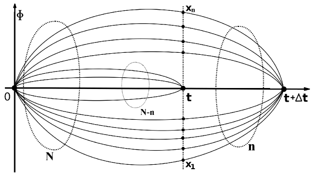
Figure 1: Schematic representation of the directed polymer paths corresponding to eq.(20)

Substituting eq.(13) into eq.(20) we get:

$$Z(N,n;t,\Delta t)=C(N,t)C(n,\Delta t)\int_{-\infty}^{+\infty}dx_{1}...dx_{n}\exp\Biggl{\{}-\frac{1}{2}\beta\sum_{a,b=1}^{n}\Bigl{[}\frac{t+\Delta t}{t\Delta t}\delta_{ab}+\frac{1}{t}A(N,t)+\frac{1}{\Delta t}A(n,\Delta t)\Bigr{]}x_{a}x_{b}\Biggr{\}}$$ (21)

Simple integration yields:

$$Z(N,n;t,\Delta t)=C(N,t)C(n,\Delta t)\Bigl{[}\frac{2\pi t\Delta t}{\beta(t+\Delta t)}\Bigr{]}^{n/2}\;\Biggl{[}1\;+\;n\frac{t\Delta t}{t+\Delta t}\Bigl{(}\frac{1}{t}A(N,t)+\frac{1}{\Delta t}A(n,\Delta t)\Bigr{)}\Biggr{]}^{-1/2}$$ (22)

Substituting here the explicit expressions (14) and (15), and taking the limit $N\to 0$ we obtain

$$\lim_{N\to 0}Z(N,n;t,\Delta t)\;=\;\Bigl{(}\frac{t}{t+\Delta t}\Bigr{)}^{n/2}\sqrt{\frac{\sqrt{\beta nu(\Delta t)^{2}}\;(t+\Delta t)}{\sin\bigl{(}\sqrt{\beta nu(\Delta t)^{2}}\bigr{)}\Bigl{[}\Delta t-\frac{1}{3}\beta nu(\Delta t)t^{2}+t\frac{\sqrt{\beta nu(\Delta t)^{2}}}{\tan\bigl{(}\sqrt{\beta nu(\Delta t)^{2}}\bigr{)}}\Bigr{]}}}$$ (23)

substituting eq.(23) into eq.(19) and redefining:

$$\Delta t\;=\;\xi\,t$$ (24)

$$\beta nu(\Delta t)^{2}\;=\;\omega$$ (25)

$$F\;=\;u\xi^{2}t^{2}\,f$$ (26)

we get the following relation for the probability distribution function $P_{t,\xi}(f)$ of the rescaled free energy $f$:

$$\int_{-\infty}^{+\infty}df\,P_{t,\xi}(f)\,\exp\{-\omega f\}\;=\;\bigl{(}1+\xi\bigr{)}^{-\frac{\omega}{2\beta u\xi^{2}t^{2}}}\frac{\omega^{1/4}\sqrt{1+\xi}}{\sqrt{\Bigl{(}\xi-\frac{\omega}{3\xi}\Bigr{)}\sin(\sqrt{\omega})\;+\;\sqrt{\omega}\cos(\sqrt{\omega})}}$$ (27)

By inverse Laplace transform in the limit when both $t\to\infty$ and $\Delta t\to\infty$ (such that the parameter ($\xi=\Delta t/t$ remains finite) we get the following universal result for the limiting two-time free energy distribution function:

$$\lim_{t\to\infty}P_{t,\xi}(f)\equiv{\cal P}_{\xi}(f)\;=\;\sqrt{1+\xi}\,\int_{-i\infty}^{+i\infty}\frac{d\omega}{2\pi i}\;\frac{\omega^{1/4}\exp\{\omega f\}}{\sqrt{\Bigl{(}\xi-\frac{\omega}{3\xi}\Bigr{)}\sin(\sqrt{\omega})\;+\;\sqrt{\omega}\cos(\sqrt{\omega})}}$$ (28)

It is interesting to note that this function (like its one-time counterpart Gorochov-Blatter ; gaussian ; replicas ) is identically equal to zero at $f>0$. Indeed, since at $f>0$ the function under the integral in the r.h.s of eq.(28) quickly goes to zero at $w\to-\infty$, the contour of integration in the complex plane can be safely shifted to $-\infty$, which means that ${\cal P}_{\xi}(f>0)\equiv 0$.

IV Two-time velocity distribution function

Velocity in the Burgers problem is given by the derivative of the free energy of the directed polymer problem:

$$v(x,t)\;=\;-\frac{\partial F(x,t)}{\partial x}\;=\;-\lim_{\epsilon\to 0}\frac{F(x+\epsilon)-F(x,t)}{\epsilon}$$ (29)

Thus, to compute the two-point velocity distribution function in terms of the directed polymers, first, keeping $\epsilon$ finite we consider specially constructed four-point object (see below), and only in the final stage of calculations we take the limit $\epsilon\to 0$.

According to the relation (6)

$$\exp\{-\beta\bigl{[}F(x+\epsilon,t)-F(x,t)\bigr{]}\}\;=\;\exp\{\beta\epsilon v(x,t)\}\;=\;\frac{Z(x+\epsilon|0;\,t)}{Z(x|0;\,t)}$$ (30)

Following the procedure described in the previous section we have:

$$\overline{\exp\bigl{\{}\beta n_{1}\epsilon v(x_{1},t)+\beta n_{2}\epsilon v(x_{2},t+\Delta t)\bigr{\}}}\;=\;$$ (31)

$$\hskip 56.9055pt=\;\lim_{N_{1},N_{2}\to 0}\overline{Z^{n_{1}}(x_{1}+\epsilon|0;\,t)\,Z^{N_{1}-n_{1}}(x_{1}|0;\,t)Z^{n_{2}}(x_{2}+\epsilon|0;\,t+\Delta t)\,Z^{N_{2}-n_{2}}(x_{2}|0;\,t+\Delta t)}$$

Introducing two-time velocity distribution function $P_{x_{1},x_{2}t,\Delta t}(v_{1},v_{2})$ the above relation can be represented as follows:

$$\int\int_{-\infty}^{+\infty}dv_{1}dv_{2}\;P_{x_{1},x_{2}t,\Delta t}(v_{1},v_{2})\exp\bigl{\{}\beta n_{1}\epsilon v_{1}+\beta n_{2}\epsilon v_{2}\bigr{\}}\;=\;\lim_{N_{1},N_{2}\to 0}\;{\cal Z}_{\epsilon}\bigl{(}N_{1},n_{1},N_{2},n_{1},x_{1},x_{2},t,\Delta t\bigr{)}$$ (32)

where

$${\cal Z}_{\epsilon}\bigl{(}N_{1},n_{1},N_{2},n_{2},x_{1},x_{2},t,\Delta t\bigr{)}\;=$$ (33)

$$\hskip 56.9055pt=\;\overline{Z^{n_{1}}(x_{1}+\epsilon|0;\,t)\,Z^{N_{1}-n_{1}}(x_{1}|0;\,t)Z^{n_{2}}(x_{2}+\epsilon|0;\,t+\Delta t)\,Z^{N_{2}-n_{2}}(x_{2}|0;\,t+\Delta t)}$$

In terms of the wave function, eq.(12)-(13),

$${\cal Z}_{\epsilon}\bigl{(}N_{1},n_{1},N_{2},n_{2},x_{1},x_{2},t,\Delta t\bigr{)}\;=$$ (34)

$$=\;\int_{-\infty}^{+\infty}\,Dy\;\int_{-\infty}^{+\infty}\,Dz\;\Psi_{N_{1}+N_{2}}\bigl{[}\underbrace{x_{1},...,x_{1}}_{N_{1}-n_{1}},\underbrace{x_{1}+\epsilon,...,x_{1}+\epsilon}_{n_{1}},y_{1},...,y_{N_{2}-n_{2}},z_{1},...,z_{n_{2}}\,|\,{\bf 0};\;t\bigr{]}\times$$

$$\hskip 99.58464pt\times\Psi^{*}_{N_{2}}\bigl{[}y_{1},...,y_{N_{2}-n_{2}},z_{1},...,z_{n_{2}}\,|\,\underbrace{x_{2},...,x_{2}}_{N_{2}-n_{2}},\underbrace{x_{2}+\epsilon,...,x_{2}+\epsilon}_{n_{2}};\,\Delta t\bigr{]}$$

where

$$\int_{-\infty}^{+\infty}\,Dy\; \equiv \;\prod_{a=1}^{N_{2}-n_{2}}\int_{-\infty}^{+\infty}dy_{a}$$ (35)

$$\int_{-\infty}^{+\infty}\,Dz\; \equiv \;\prod_{a=1}^{n_{2}}\int_{-\infty}^{+\infty}dz_{a}$$

Schematically the expression in eq.(34) is represented in Figure 2.

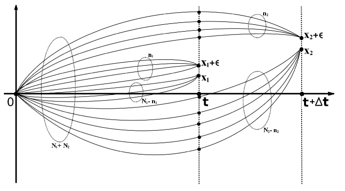
Figure 2: Schematic representation of the directed polymer paths corresponding to eq.(34)

Substituting the explicit expressions for the wave function (13) into eq.(34) we get:

$${\cal Z}_{\epsilon}\bigl{(}N_{1},n_{1},N_{2},n_{2},x_{1},x_{2},t,\Delta t\bigr{)}\;=\;C(N_{1}+N_{2},t)\,C(N_{2},\Delta t)\times$$

$$\times\int_{-\infty}^{+\infty}\,Dy\;\int_{-\infty}^{+\infty}\,Dz\;\exp\Biggl{\{}-\frac{\beta}{2t}\Biggl{[}(N_{1}-n_{1})x_{1}^{2}+n_{1}(x_{1}+\epsilon)^{2}+\sum_{a=1}^{N_{2}-n_{2}}y_{a}^{2}+\sum_{a=1}^{n_{2}}z_{a}^{2}\Biggr{]}\,-$$

$$\hskip 65.44133pt-\frac{\beta}{2t}A(N_{1}+N_{2},t)\Biggl{[}(N_{1}-n_{1})x_{1}+n_{1}(x_{1}+\epsilon)+\sum_{a=1}^{N_{2}-n_{2}}y_{a}+\sum_{a=1}^{n_{2}}z_{a}\Biggr{]}^{2}\,-$$

$$\hskip 65.44133pt-\frac{\beta}{2\Delta t}\Biggl{[}\sum_{a=1}^{N_{2}-n_{2}}(y_{a}-x_{2})^{2}+\sum_{a=1}^{n_{2}}(z_{a}-x_{2}-\epsilon)^{2}\Biggr{]}\,-$$

$$\hskip 65.44133pt-\frac{\beta}{2\Delta t}A(N_{2},\Delta t)\Biggl{[}\sum_{a=1}^{N_{2}-n_{2}}(y_{a}-x_{2})+\sum_{a=1}^{n_{2}}(z_{a}-x_{2}-\epsilon)\Biggr{]}^{2}\,+$$

$$\hskip 65.44133pt+\frac{\beta}{\Delta t}B(N_{2},\Delta t)\Bigl{(}\sum_{a=1}^{N_{2}-n_{2}}y_{a}+\sum_{a=1}^{n_{2}}z_{a}\Bigr{)}\Bigl{[}(N_{2}-n_{2})x_{2}+n_{2}(x_{2}+\epsilon)\Bigr{]}\Biggr{\}}$$ (36)

where $A(N,t)$, $B(N,t)$ and $C(N,t)$ are given in eqs.(14)-(16). Introducing $N_{2}$-component vector ${\boldsymbol{\chi}}=\{y_{1},...,y_{N_{2}-n_{2}},z_{1},...,z_{n_{2}}\}$ after simple algebra we get

$${\cal Z}_{\epsilon}\bigl{(}N_{1},n_{1},N_{2},n_{2},x_{1},x_{2},t,\Delta t\bigr{)} = C(N_{1}+N_{2},t)\,C(N_{2},\Delta t)\times$$ (37)

$$\times \Biggl{[}\prod_{a=1}^{N_{2}}\int_{-\infty}^{+\infty}d\chi_{a}\Biggr{]}\;\exp\Biggl{\{}-\frac{1}{2}\sum_{a,b=1}^{N_{2}}T_{ab}\chi_{a}\chi_{b}\;+\;\sum_{a=1}^{N_{2}}L_{a}\chi_{a}-\frac{1}{2}\beta G\Biggr{\}}$$

where

$$G = \frac{1}{t}\bigl{[}n_{1}(x_{1}+\epsilon)^{2}+(N_{1}-n_{1})x_{1}^{2}\bigr{]}\;+\;\frac{1}{\Delta t}\bigl{[}n_{2}(x_{2}+\epsilon)^{2}+(N_{2}-n_{2})x_{2}^{2}\bigr{]}\;+$$ (38)

$$+ \frac{1}{t}A(N_{1}+N_{2},t)\bigl{(}N_{1}x_{1}+n_{1}\epsilon\bigr{)}^{2}\;+\;\frac{1}{\Delta t}A(N_{2},\Delta t)\bigl{(}N_{2}x_{2}+n_{2}\epsilon\bigr{)}^{2}$$

and

$$T_{ab} = \gamma\,\delta_{ab}\;+\;\kappa$$ (39)

$$\gamma = \beta\frac{t+\Delta t}{t\Delta t}$$ (40)

$$\kappa = \frac{\beta}{t}A(N_{1}+N_{2},t)\;+\;\frac{\beta}{\Delta t}A(N_{2},\Delta t)$$ (41)

$$L_{a} = L\;+\;X_{a}$$ (42)

$$L = -\frac{\beta}{t}A(N_{1}+N_{2},t)\bigl{(}N_{1}x_{1}+n_{1}\epsilon\bigr{)}\;+\;\frac{\beta}{\Delta t}\bigl{[}A(N_{2},\Delta t)+B(N_{2},\Delta t)\bigr{]}\bigl{(}N_{2}x_{2}+n_{2}\epsilon)$$ (43)

$$X_{a} = \left\{\begin{array}[]{ll}x_{2}+\epsilon,&\mbox{for $a=1,...,n_{2}$}\\ x_{2},&\mbox{for $a=n_{2}+1,...,N_{2}$}\end{array}\right.$$ (46)

Simple integration over $\chi$’s in eq.(37) yields:

$${\cal Z}_{\epsilon}\bigl{(}N_{1},n_{1},N_{2},n_{2},x_{1},x_{2},t,\Delta t\bigr{)}\; = \;C(N_{1}+N_{2},t)\,C(N_{2},\Delta t)\times$$ (47)

$$\times \exp\Biggl{\{}-\frac{1}{2}\beta G-\frac{1}{2}\mbox{Tr}\,\ln\hat{T}\;+\;\frac{1}{2}\sum_{a,b=1}^{N_{2}}L_{a}L_{b}\hat{T}^{-1}_{ab}\Biggr{\}}$$

where

$$\mbox{Tr}\,\ln\hat{T} = N_{2}\ln\gamma\;+\;\ln\Bigl{(}1\;+\;N_{2}\frac{\kappa}{\gamma}\Bigr{)}$$ (48)

$$\hat{T}^{-1}_{ab} = \frac{1}{\gamma}\delta_{ab}\;-\;\frac{\kappa}{\gamma\bigl{(}\gamma+N_{2}\kappa\bigr{)}}$$ (49)

Simple calculations yield:

$${\cal Z}_{\epsilon}\bigl{(}N_{1},n_{1},N_{2},n_{2},x_{1},x_{2},t,\Delta t\bigr{)}\;=\;C(N_{1}+N_{2},t)\,C(N_{2},\Delta t)\;\times$$

$$\hskip 28.45274pt\times\exp\Biggl{\{}-\frac{1}{2}\beta G-\frac{1}{2}N_{2}\ln\gamma-\frac{1}{2}\ln\Bigl{(}1+N_{2}\frac{\kappa}{\gamma}\Bigr{)}-\frac{L^{2}N_{2}}{2(\gamma+N_{2}\kappa)}+\frac{\beta L}{\gamma\Delta t}\bigl{(}N_{2}x_{2}+n_{2}\epsilon\bigr{)}-$$

$$\hskip 28.45274pt-\frac{\beta\kappa N_{2}(N_{2}x_{2}+n_{2}\epsilon)}{\gamma\Delta t(\gamma+N_{2}\kappa)}-\frac{\beta^{2}\kappa(N_{2}x_{2}+n_{2}\epsilon)^{2}}{2\gamma(\Delta t)^{2}(\gamma+N_{2}\kappa)}+\frac{\beta^{2}}{2\gamma(\Delta t)^{2}}\Bigl{[}(N_{2}-n_{2})x_{2}^{2}+n_{2}(x_{2}+\epsilon)^{2}\Bigr{]}\Biggr{\}}$$ (50)

Next step of the calculations is to take the limits $N_{1,2}\to 0$. Using explicit expressions (14)-(16), (38), (41) and (43), one easily finds:

$$\lim_{N\to 0}C(N,t) = 1$$ (51)

$$\lim_{N\to 0}A(N,t) = -\frac{1}{3}\beta ut^{2}$$ (52)

$$\lim_{N\to 0}B(N,t) = \frac{1}{2}\beta ut^{2}$$ (53)

$$\lim_{N_{1},N_{2}\to 0}\beta G = \frac{\beta n_{1}\epsilon}{t}(2x_{1}+\epsilon)+\frac{\beta n_{2}\epsilon}{\Delta t}(2x_{2}+\epsilon)-\frac{1}{3}(\beta n_{1}\epsilon)^{2}ut-\frac{1}{3}(\beta n_{2}\epsilon)^{2}u\Delta t$$ (54)

$$\lim_{N_{1},N_{2}\to 0}L = \frac{1}{3}\beta^{2}n_{1}\epsilon ut+\frac{1}{6}\beta^{2}n_{2}\epsilon u\Delta t$$ (55)

$$\lim_{N_{1},N_{2}\to 0}\kappa = -\frac{1}{3}\beta^{2}u(t+\Delta t)$$ (56)

Substituting the above limiting values into eq.(50) we get

$$\lim_{N_{1,2}\to 0}{\cal Z}_{\epsilon}\bigl{(}N_{1},n_{1},N_{2},n_{2},x_{1},x_{2},t,\Delta t\bigr{)}\;\equiv\;Z_{\epsilon}\bigl{(}n_{1},n_{2},x_{1},x_{2},t,\Delta t\bigr{)}\;=$$

$$=\exp\Biggl{\{}-\frac{\beta n_{1}\epsilon}{2t}(2x_{1}+\epsilon)-\frac{\beta n_{2}\epsilon}{2(t+\Delta t)}(2x_{2}+\epsilon)+\frac{1}{6}(\beta n_{1}\epsilon)^{2}ut+\frac{1}{6}(\beta n_{2}\epsilon)^{2}u(t+\Delta t)+\frac{(\beta n_{1}\epsilon)(\beta n_{2}\epsilon)ut^{2}}{3(t+\Delta t)}\Biggr{\}}$$ (57)

Substituting the above result into eq.(32) and introducing notations $\beta n_{1,2}\epsilon\;=\;s_{1,2}$ in the limit $\epsilon\to 0$ we obtain:

$$\int\int_{-\infty}^{+\infty}dv_{1}dv_{2}\;P_{x_{1},x_{2}t,\Delta t}(v_{1},v_{2})\exp\bigl{\{}s_{1}v_{1}+s_{2}v_{2}\bigr{\}}\;=\;$$

$$=\exp\Biggl{\{}-\frac{x_{1}}{t}s_{1}-\frac{x_{2}}{t+\Delta t}s_{2}+\frac{1}{6}uts_{1}^{2}+\frac{1}{6}u(t+\Delta t)s_{2}^{2}+\frac{ut^{2}}{3(t+\Delta t)}s_{1}s_{2}\ \Biggr{\}}$$ (58)

Redefining

$$s_{1} = \sqrt{\frac{3}{ut}}\;\omega_{1}$$ (59)

$$s_{2} = \sqrt{\frac{3}{u(t+\Delta t)}}\;\omega_{2}$$ (60)

$$v_{1} = -\frac{x_{1}}{t}\;+\;\sqrt{\frac{1}{3}ut}\;\tilde{v}_{1}$$ (61)

$$v_{2} = -\frac{x_{2}}{t+\Delta t}\;+\;\sqrt{\frac{1}{3}u(t+\Delta t)}\;\tilde{v}_{2}$$ (62)

$$\Delta t = \xi\,t$$ (63)

we get the following relation for the probability distribution function ${\cal P}_{\xi}\bigl{(}\tilde{v}_{1},\,\tilde{v}_{2}\bigr{)}$ for the rescaled velocities $\tilde{v}_{1}$ and $\tilde{v}_{2}$, eqs.(61)-(62):

$$\int\int_{-\infty}^{+\infty}d\tilde{v}_{1}\tilde{v}_{2}{\cal P}_{\xi}\bigl{(}\tilde{v}_{1},\,\tilde{v}_{2}\bigr{)}\exp\bigl{\{}\omega_{1}\tilde{v}_{1}+\omega_{2}\tilde{v}_{2}\bigr{\}}\;=\;\exp\Bigl{\{}\frac{1}{2}\omega_{1}^{2}+\frac{1}{2}\omega_{2}^{2}+\frac{\omega_{1}\omega_{2}}{(1+\xi)^{3/2}}\Bigr{\}}$$ (64)

Performing simple inverse Laplace transformation

$${\cal P}_{\xi}\bigl{(}\tilde{v}_{1},\,\tilde{v}_{2}\bigr{)}\;=\;\int\int_{-i\infty}^{+i\infty}\frac{d\omega_{1}d\omega_{2}}{(2\pi i)^{2}}\;\exp\Bigl{\{}\frac{1}{2}\omega_{1}^{2}+\frac{1}{2}\omega_{2}^{2}+\frac{\omega_{1}\omega_{2}}{(1+\xi)^{3/2}}-\omega_{1}\tilde{v}_{1}-\omega_{2}\tilde{v}_{2}\Bigr{\}}$$ (65)

one eventually obtain the following very simple result for the two-time velocities distribution function:

$${\cal P}_{\xi}\bigl{(}\tilde{v}_{1},\,\tilde{v}_{2}\bigr{)}\;=\;\frac{1}{2\pi}\sqrt{\frac{(1+\xi)^{3}}{(1+\xi)^{3}-1}}\;\exp\Biggl{\{}-\frac{(1+\xi)^{3}}{2\bigl{[}(1+\xi)^{3}-1\bigr{]}}\Bigl{(}\tilde{v}_{1}^{2}-2\frac{\tilde{v}_{1}\tilde{v}_{2}}{(1+\xi)^{3/2}}+\tilde{v}_{2}^{2}\Bigr{)}\Biggr{\}}$$ (66)

where $\xi=\Delta t/t$ is the reduced separation time parameter.

One can easily check that in the limit of infinite separation time, $\xi\to\infty$, the distributions of two velocities are getting independent:

$$\lim_{\xi\to\infty}{\cal P}_{\xi}\bigl{(}\tilde{v}_{1},\,\tilde{v}_{2}\bigr{)}\;=\;\frac{1}{2\pi}\;\exp\Bigl{\{}-\frac{1}{2}\tilde{v}_{1}^{2}-\frac{1}{2}\tilde{v}_{2}^{2}\Bigr{\}}$$ (67)

while in the opposite limit of coinciding times, $\xi\to 0$, one finds

$${\cal P}_{0}\bigl{(}\tilde{v}_{1},\,\tilde{v}_{2}\bigr{)}\;=\;\frac{1}{\sqrt{2\pi}}\;\exp\Bigl{\{}-\frac{1}{2}\tilde{v}_{1}^{2}\Bigr{\}}\;\delta\bigl{(}\tilde{v}_{1}-\tilde{v}_{2}\bigr{)}$$ (68)

as it should be.

Besides, using the exact result, eq.(66) one can easily compute the time dependence of the two velocities correlation function:

$$\langle\tilde{v}_{1}\tilde{v}_{2}\rangle\;=\;(1+\xi)^{-3/2}$$ (69)

as well as the probability distribution function for the velocities difference $\tilde{v}\equiv\tilde{v}_{2}-\tilde{v}_{1}$:

$${\cal P}_{\xi}\bigl{(}\tilde{v}\bigr{)}\;=\;\frac{1}{2\pi}\sqrt{\frac{(1+\xi)^{3/2}}{4\pi\bigl{[}(1+\xi)^{3/2}-1\bigr{]}}}\;\exp\Biggl{\{}-\frac{(1+\xi)^{3/2}}{4\bigl{[}(1+\xi)^{3/2}-1\bigr{]}}\,\tilde{v}^{2}\Biggr{\}}$$ (70)

V Conclusions

In this paper we have considered the problem of velocity distribution functions in the Burgulence problem in terms of the toy Gaussian model of (1+1) directed polymers. In particular the exact result for the two-time free energy, eq.(28), and two-time velocity distribution functions, eq.(66) has been derived. Of course the considered system is too far from the realistic one. Nevertheless, it has one important advantage: being exactly solvable, some of its statistical properties are rather non-trivial. All that, in my view, makes this model to be rather useful tool for testing new ideas and various technical aspects of the calculations (like the replica technique considered in this paper).

Following the proposed route, the next step would be to consider the model with finite range correlations of the random potentials. Of course, one can not hope to get exact results here. In terms of the replica approach, first of all, one is facing the problem of $N$-particle quantum bosons with attractive finite range interactions whose solution is not known. Nevertheless even the qualitative understanding of the structure of the $N$-particle wave function of this system (which at the qualitative level might be not so much different from that of the Bethe ansatz solution for the $\delta$-correlated potentials) could hopefully be sufficient to get some understanding of the velocity statistics in the Burgulence problem.

References

(1) M.Kardar, G.Parisi, Y-C.Zhang,
Phys. Rev. Lett. 56, 889 (1986)
(2) T. Halpin-Healy and Y-C. Zhang,
Phys. Rep. 254, 215 (1995).
(3) J.M. Burgers, The Nonlinear
Diffusion Equation (Reidel, Dordrecht, (1974)).
(4) M. Kardar,
”Statistical physics of fields” (Cambridge: Cambridge University Press, (2007))
(5) D.A. Huse, C.L. Henley, and D.S. Fisher,
Phys. Rev. Lett. 55, 2924 (1985).
(6) D.A. Huse and C.L. Henley,
Phys. Rev. Lett. 54, 2708 (1985).
(7) M. Kardar and Y-C. Zhang,
Phys. Rev. Lett. 58, 2087 (1987).
(8) M. Kardar,
Nucl. Phys. B 290, 582 (1987).
(9) J. P. Bouchaud and H. Orland,
J. Stat. Phys. 61, 877 (1990)
(10) E. Brunet and B. Derrida,
Phys. Rev. E 61, 6789 (2000)
(11) K. Johansson,
Comm. Math. Phys. 209, 437 (2000)
(12) M. Prahofer and H. Spohn
J. Stat. Phys. 108, 1071 (2002)
(13) P. L. Ferrari and H. Spohn,
Comm. Math. Phys. 265, 1 (2006)
(14) T.Sasamoto and H.Spohn,
Phys. Rev. Lett. 104, 230602 (2010)
(15) T.Sasamoto and H.Spohn,
Nucl. Phys. B834, 523 (2010)
(16) T.Sasamoto and H.Spohn,
J. Stat. Phys. 140, 209 (2010)
(17) G.Amir, I.Corwin and J.Quastel,
Comm. Pure Appl. Math. 64, 466 (2011)
(18) V.Dotsenko and B.Klumov,
J.Stat.Mech. P03022 (2010)
(19) V.Dotsenko,
EPL, 90,20003 (2010)
(20) V.Dotsenko,
J.Stat.Mech. P07010 (2010)
(21) P.Calabrese, P. Le Doussal and A.Rosso,
EPL, 90,20002 (2010);
(22) P.Calabrese and P. Le Doussal,
Phys. Rev. Lett. 106, 250603 (2011);
arXiv:1204.2607
(23) V.Dotsenko,
J. Stat. Mech. P02012 (2012)
(24) V.Dotsenko,
J. Stat. Mech. P11014 (2012)
(25) T.Gueudré and P. Le Doussal,
EPL, 100, 26006 (2012).
(26) I. Corwin,
”The Kardar-Parisi-Zhang equation and the universality class”,
arXiv:1106.1338, Random Matrices: Theory Appl. 1, 1130001 (2012)
(27) A.Borodin, I.Corwin and P.Ferrari,
Free energy fluctuations for directed polymers in random media in 1+1 dimension,
arXiv:1204.1024 (2012)
(28) S. Prolhac and H. Spohn,
J.Stat.Mech. P01031 (2011)