Inference for Generalized Linear Models via Alternating Directions and Bethe Free Energy Minimization

Abstract

Generalized Linear Models (GLMs), where a random vector $\mathbf{x}$ is observed through a noisy, possibly nonlinear, function of a linear transform $\mathbf{z}=\mathbf{A}\mathbf{x}$, arise in a range of applications in nonlinear filtering and regression. Approximate Message Passing (AMP) methods, based on loopy belief propagation, are a promising class of approaches for approximate inference in these models. AMP methods are computationally simple, general, and admit precise analyses with testable conditions for optimality for large i.i.d. transforms $\mathbf{A}$. However, the algorithms can diverge for general $\mathbf{A}$. This paper presents a convergent approach to the generalized AMP (GAMP) algorithm based on direct minimization of a large-system limit approximation of the Bethe Free Energy (LSL-BFE). The proposed method uses a double-loop procedure, where the outer loop successively linearizes the LSL-BFE and the inner loop minimizes the linearized LSL-BFE using the Alternating Direction Method of Multipliers (ADMM). The proposed method, called ADMM-GAMP, is similar in structure to the original GAMP method, but with an additional least-squares minimization. It is shown that for strictly convex, smooth penalties, ADMM-GAMP is guaranteed to converge to a local minimum of the LSL-BFE, thus providing a convergent alternative to GAMP that is stable under arbitrary transforms. Simulations are also presented that demonstrate the robustness of the method for non-convex penalties as well.

I Introduction

Consider the problem of estimating a random vector $\mathbf{x}\in{\mathbb{R}}^{n}$ from observations $\mathbf{y}\in{\mathbb{R}}^{m}$ as shown in Fig. 1. The unknown vector is assumed to have a prior density of the form $p(\mathbf{x})=\mathrm{e}^{-f_{x}(\mathbf{x})}$ and the observations $\mathbf{y}\in{\mathbb{R}}^{m}$ are described by a likelihood function of the form $p(\mathbf{y}|\mathbf{x})=\mathrm{e}^{-f_{z}(\mathbf{A}\mathbf{x},\mathbf{y})}$ for some known transform $\mathbf{A}\in{\mathbb{R}}^{m\times n}$. In statistics, this model is a special case of a generalized linear model (GLM) [1, 2] and arises in a range of applications including statistical regression, filtering, inverse problems, and nonlinear forms of compressed sensing. The posterior density of $\mathbf{x}$ given $\mathbf{y}$ in the GLM model is given by

$$p_{\mathbf{x}|\mathbf{y}}(\mathbf{x}|\mathbf{y})=\frac{1}{Z(\mathbf{y})}\exp\left[-f_{x}(\mathbf{x})-f_{z}(\mathbf{A}\mathbf{x},\mathbf{y})\right],$$ (1)

where $Z(\mathbf{y})$ is a normalization constant. In the sequel, we will often omit the dependence on $\mathbf{y}$ and simply write

$$p_{\mathbf{x}|\mathbf{y}}(\mathbf{x}|\mathbf{y})=\frac{1}{Z}\exp\left[-f_{x}(\mathbf{x})-f_{z}(\mathbf{A}\mathbf{x})\right],$$ (2)

so that the dependence on $\mathbf{y}$ in the function $f_{z}(\cdot)$ and the normalization constant $Z$ is implicit. In this work, we consider the inference problem of estimating the posterior marginal distributions, $p_{x_{j}|\mathbf{y}}(x_{j}|\mathbf{y})$. From these posterior marginals, one can compute the posterior means and variances

$$\widehat{x}_{j} \triangleq \mathbb{E}(x_{j}|\mathbf{y}),$$ (3a)

$$\tau_{x_{j}} \triangleq \mbox{var}(x_{j}|\mathbf{y}).$$ (3b)

We study this inference problem in the case where the functions $f_{x}$ and $f_{z}$ are separable, in that they are of the form

$$f_{x}(\mathbf{x}) = \sum_{j=1}^{n}f_{x_{j}}(x_{j}),$$ (4a)

$$f_{z}(\mathbf{z}) = \sum_{i=1}^{m}f_{z_{i}}(z_{i}),$$ (4b)

for some scalar functions $f_{x_{j}}$ and $f_{z_{i}}$. The separability assumption (4a) corresponds to the components in $\mathbf{x}$ being a priori independent. Recalling the implicit dependence of $f_{z}$ on $\mathbf{y}$, the separability assumption (4b) corresponds to the observations $\mathbf{y}$ being conditionally independent given the transform outputs $\mathbf{z}\triangleq\mathbf{A}\mathbf{x}$.

Figure 1: Generalized Linear Model (GLM) where an unknown random vector $\mathbf{x}$ is observed via a linear transform followed by componentwise likelihood to yield a measurement vector $\mathbf{y}$.

For posterior densities of the form (2), there are several computationally efficient methods to find the maximum a posteriori (MAP) estimate, which is given by

$$\widehat{\mathbf{x}}=\mathop{\mathrm{arg\,max}}_{\mathbf{x}}p_{\mathbf{x}|\mathbf{y}}(\mathbf{x}|\mathbf{y})=\mathop{\mathrm{arg\,min}}_{\mathbf{x}}\left[f_{x}(\mathbf{x})+f_{z}(\mathbf{A}\mathbf{x})\right].$$ (5)

Under the separability assumptions (4), the MAP minimization (5) admits a factorizable dual decomposition that can be exploited by a variety of approaches, including variants of the iterative shrinkage and thresholding algorithm (ISTA) [3, 4, 5, 6, 7, 8] and the alternating direction method of multipliers (ADMM) [9, 10, 11, 12].

In contrast, the inference problem of estimating the posterior marginals $p(x_{j}|\mathbf{y})$ and the corresponding minimum mean squared error (MMSE) estimates (3a) is often more difficult—even in the case when $f_{x}$ and $f_{z}$ are convex. As a simple example, consider the case where $f_{x}(\mathbf{x})=0$ and each $f_{z_{i}}(z_{i})$ constrains $z_{i}$ to belong to some interval, so that $f_{z}(\mathbf{A}\mathbf{x})$ constrains $\mathbf{x}$ to belong to some polytope. The MAP estimate (5) is then given by any point in the polytope. Such a point can can be computed via a linear program. However, the MMSE estimate (3a) is the centroid of the polytope which is, in general, #P-hard to compute [13].

GLM inference methods often use a penalized quasi-likelihood method [14] or some form of Gibbs sampling [15, 16]. In recent years, Bayesian forms of approximate message passing (AMP) have been considered as a potential alternate class of methods for approximate inference in GLMs [17, 18, 19, 20, 21, 22]. AMP methods are based on Gaussian and quadratic approximations to loopy belief propagation (loopy BP) in graphical models and are both computationally simple and applicable to arbitrary separable penalty functions $f_{x}$ and $f_{z}$. In addition, for certain large i.i.d. transforms $\mathbf{A}$, they have the benefit that the behavior of the algorithm can be exactly predicted by a state evolution analysis, which then provides testable conditions for Bayes optimality [23, 22, 24].

Unfortunately, for general $\mathbf{A}$, AMP methods may diverge [25, 26]—a situation that is not surprising given that AMP is based on loopy BP, which also may diverge. Several recent modifications have been proposed to improve the stability of AMP, including damping [25], sequential updating [27], and adaptive damping [28]. However, while these methods appear to perform well empirically, little has been proven rigorously about their convergence.

The main goal of this paper is to provide a provably convergent approach to AMP. We focus on the generalized AMP (GAMP) method of [22], which allows arbitrary separable functions for both $f_{x}$ and $f_{z}$. Our approach to stabilizing GAMP is based on reconsidering the inference problem as a type of free-energy minimization. Specifically, it is known that GAMP can be considered as an iterative procedure for minimizing a large-system-limit approximation of the so-called Bethe Free Energy (BFE) [29, 30], which we abbreviate as “LSL-BFE” in the sequel. The BFE also plays a central role in loopy BP [31], and we review both the BFE and LSL-BFE in Section III.

In contrast to GAMP, which implicitly minimizes the LSL-BFE through an approximation of the sum-product algorithm, our proposed approach explicitly minimizes the LSL-BFE. We propose a double-loop algorithm, similar to the well-known Convex Concave Procedure (CCCP) [32]. Specifically, the outer loop of our method successively approximates the LSL-BFE by partially linearizing the LSL-BFE around the current belief estimate, while the inner loop minimizes the linearized LSL-BFE using ADMM [9]. Similar applications of ADMM have also been proposed for related free-energy minimizations [33, 34]. Interestingly, our proposed double-loop algorithm, which we dub ADMM-GAMP, is similar in structure to the original GAMP method of [22], but with an additional least squares optimization. We discuss these differences in detail in Section VIII.

Our main theoretical result shows that, for strictly convex penalties, the proposed ADMM-GAMP algorithm is guaranteed to converge to at least a local minimum of the LSL-BFE. In this way, we obtain a variant of the GAMP method with a provable convergence guarantee for arbitrary transforms $\mathbf{A}$. In addition, using hardening arguments similar to [35, 36], we show that our ADMM-GAMP can also be applied to the MAP estimation problem, in which case we can obtain global convergence for strictly convex, smooth penalties. Also, while our theory requires convex penalties, we present simulations that show robust behavior even in non-convex cases.

II The GLM and Examples

Before describing our optimization approach, it is useful to briefly provide some examples of the model (1) to illustrate the generality of the framework. As a first simple example, consider a simple linear model

$$\mathbf{y}=\mathbf{A}\mathbf{x}+\mathbf{\epsilon},,$$ (6)

where $\mathbf{A}$ is a known matrix, $\mathbf{x}$ is an unknown vector and $\epsilon$ is a noise vector. In statistics, $\mathbf{A}$ would be the data matrix with predictors, $\mathbf{x}$ would be the vector of regression coefficients, $\mathbf{y}$ the vector of target or response variables and $\mathbf{\epsilon}$ would represent the model errors. To place this model in the framework of this paper, we must impose a prior $p(\mathbf{x})$ on $\mathbf{x}$ and model the noise $\mathbf{\epsilon}$ as a random vector independent of $\mathbf{A}$ and $\mathbf{x}$. Under these assumptions, the posterior density of $\mathbf{x}$ given $\mathbf{y}$ will be of the form (1) if we define

$$f_{x}(\mathbf{x}):=-\ln p(\mathbf{x}),\quad f_{z}(\mathbf{z}):=-\ln p(\mathbf{y}|\mathbf{z})=-\ln p_{\epsilon}(\mathbf{y}-\mathbf{z}).$$ (7)

The separability assumption (4) will be valid if the components of $x_{j}$ are $w_{i}$ are independent so the prior and noise density factorizes as

$$p(\mathbf{x})=\prod_{j=1}^{n}p(x_{j}),\quad p(\mathbf{\epsilon})=\prod_{i=1}^{m}p(\epsilon_{i}).$$

If the output noise $\mathbf{\epsilon}$ is Gaussian with independent components $\epsilon_{i}\sim{\mathcal{N}}(0,\sigma^{2}_{\epsilon})$, the output factor $f_{z}(\mathbf{z})$ in (7) has a quadratic cost,

$$f_{z}(\mathbf{z})=\frac{1}{2\sigma^{2}_{\epsilon}}\|\mathbf{y}-\mathbf{z}\|^{2}.$$

Similarly, if $\mathbf{x}$ has a Gaussian prior with ${\mathcal{N}}(0,\sigma^{2}_{x}\mathbf{I})$, the input factor $f_{x}(\mathbf{x})$ will be given by

$$f_{x}(\mathbf{x})=\frac{1}{2\sigma^{2}_{\epsilon}}\|\mathbf{x}\|^{2}.$$

Note that the estimation in this quadratic case would be given by standard least squares estimation.

However, much more general models are possible. For example, for Bayesian forms of compressed sensing problems [37], one can impose a sparse prior $p(\mathbf{x})$ such as a Bernoulli-Gaussian or a heavy-tailed density.

Also, for the output, any likelihood $p(\mathbf{y}|\mathbf{z})$ that factorizes as $\prod_{i}p(y_{i}|z_{i})$ can be incorporated. This model would occur, for example, under any output nonlinearities as considered in [38],

$$y_{i}=\phi_{i}(z_{i})+\epsilon_{i},$$

where $\phi_{i}(z_{i})$ is a known, nonlinear function and $\epsilon_{i}$ is noise. The model can also include logistic regression [39] where $y_{i}\in\{0,1\}$ is a binary class variable and

$$P(y_{i}=1|z_{i})=1-P(y_{i}=0|z_{i})=\sigma(z_{i}),$$

for some sigmoidal function $\sigma(z)$. One-bit and quantized compressed sensing [40] as well as Poisson output models [41] can also be easily modeled.

III Bethe Free Energy Minimization

We next provide a brief review of the Bethe Free Energy (BFE) minimization approach to estimation of marginal densities in GLMs. A more complete treatment of this topic, along with related ideas in variational inference, can be found in [31, 42].

For a generic density $p(\mathbf{x}|\mathbf{y})$, exact computation of the marginal densities $p(x_{j}|\mathbf{y})$ is difficult, because it involves a potentially high-dimensional integration. BFE minimization provides an approximate approach to marginal density computation for the case when the joint density admits a factorizable structure of the form

$$p(\mathbf{x}|\mathbf{y})\propto\prod_{\ell=1}^{L}\psi_{\ell}(\mathbf{x}_{\alpha(\ell)}|\mathbf{y}),$$ (8)

where, for each $\ell$, $\mathbf{x}_{\alpha(\ell)}$ is a sub-vector of $\mathbf{x}$ created from indices in the subset $\alpha(\ell)$ and $\psi_{\ell}$ is a potential function on that sub-vector. In this case, BFE minimization aims to compute the vectors of densities

$$\mathbf{b} \triangleq [b_{1},\dots,b_{n}]^{\text{\sf T}}\quad\text{and}\quad\mathbf{q}\triangleq[q_{1},\dots,q_{L}]^{\text{\sf T}},$$

where $b_{j}(x_{j})$ represents an estimate of the marginal density $p(x_{j}|\mathbf{y})$ and where $q_{\ell}(\mathbf{x}_{\alpha(\ell)})$ represents an estimate of the joint density $p(\mathbf{x}_{\alpha(\ell)}|\mathbf{y})$ on the sub-vector $\mathbf{x}_{\alpha(\ell)}$. These density estimates, often called “beliefs,” are computed using an optimization of the form

$$\big{(}\widehat{\mathbf{b}},\widehat{\mathbf{q}}\big{)}=\mathop{\mathrm{arg\,min}}_{(\mathbf{b},\mathbf{q})\in E}J(\mathbf{b},\mathbf{q}),$$ (9)

where $J(\mathbf{b},\mathbf{q})$ is the BFE given by

$$J(\mathbf{b},\mathbf{q})\triangleq\sum_{\ell=1}^{L}D(q_{\ell}\|\psi_{\ell})+\sum_{j=1}^{n}(n_{j}-1)H(b_{j});$$ (10)

where $D(q_{\ell}\|\psi_{\ell})$ is the KL divergence,

$$D(a\|b)\triangleq\int a(x)\ln\left[\frac{a(x)}{b(x)}\right]\mathrm{\,d}x;$$ (11)

where $H(b_{j})$ is the entropy or differential entropy; and where (for each $j$) $n_{j}$ is the number of factors $\ell$ such that $j\in\alpha(\ell)$. The BFE minimization (9) is performed over the set $E$ of all $(\mathbf{b},\mathbf{q})$ whose components satisfy a particular “matching” condition: for each $j\in\alpha(\ell)$, the marginal density of $x_{j}$ within the belief $q_{\ell}(\mathbf{x}_{\alpha(\ell)})$ must agree with the belief $b_{j}(x_{j})$. That is, the set $E$ contains all $(\mathbf{b},\mathbf{q})$ such that

$$\int q_{\ell}(\mathbf{x}_{\alpha(\ell)})\mathrm{\,d}\mathbf{x}_{\alpha(\ell)\backslash j}=b_{j}(x_{j}),\mbox{ for all }\ell,j,$$ (12)

where the integration is over the components in the sub-vector $\mathbf{x}_{\alpha(\ell)}$ holding $x_{j}$ constant. Note that $E$ imposes a set of linear constraints on the belief vectors $\mathbf{b}$ and $\mathbf{q}$.

The BFE minimization exactly recovers the true marginals in certain cases (e.g., when the factor graph has no cycles) and provides good estimates in many other scenarios as well; see [42] for a complete discussion. In addition, due to its separable structure, the BFE can be typically minimized “locally,” by solving a set of minimizations over the densities $\mathbf{b}$ and $\mathbf{q}$. When the cardinalities of the subsets $\alpha(\ell)$ are small, these local minimizations may involve much less computation than directly calculating the marginals of the full joint density $p(\mathbf{x}|\mathbf{y})$. In fact, the classic result of [31] is that loopy belief propagation can be interpreted precisely as one type of iterative local minimization of the BFE.

For the GLM in Section I, the separability assumption (4) allows us to write the density (2) in the factorized form (8) using the $L=n+m$ potentials

$$\psi_{j}(x_{j}) = \exp(-f_{x_{j}}(x_{j})),~{}j=1,\ldots,n,$$ (13a)

$$\psi_{n+i}(\mathbf{x}) = \exp(-f_{z_{i}}(\mathbf{a}_{i}^{\text{\sf T}}\mathbf{x})),~{}i=1,\ldots,m,$$ (13b)

where $\mathbf{a}_{i}^{\text{\sf T}}$ is the $i$-th row of $\mathbf{A}$. Note that, if $\mathbf{A}$ is a non-sparse matrix, then $f_{z_{i}}(\mathbf{a}_{i}^{\text{\sf T}}\mathbf{x})$ depends on all components in the vector $\mathbf{x}$. In this case, the application of traditional loopy BP—as described for example in [43]—does not generally yield a significant computational improvement.

The GAMP algorithm from [22] can be seen as an approximate BFE minimization method for GLMs with possibly dense transforms $\mathbf{A}$. Specifically, it was shown in [29] that the stationary points of GAMP coincide with the local minima of the constrained optimization

$$(\widehat{b}_{x},\widehat{b}_{z}) \triangleq \mathop{\mathrm{arg\,min}}_{b_{x},b_{z}}J(b_{x},b_{z})\text{~{}such that}$$ (14b)

$$\mathbb{E}(\mathbf{z}|b_{z})=\mathbf{A}\mathbb{E}(\mathbf{x}|b_{x})$$

where $b_{x}$ and $b_{z}$ are product densities, i.e.,

$$b_{x}(\mathbf{x})=\prod_{j=1}^{n}b_{x_{j}}(x_{j}),\qquad b_{z}(\mathbf{z})=\prod_{i=1}^{m}b_{z_{i}}(z_{i}),$$ (15)

and the objective function $J(b_{x},b_{z})$ is given by

$$J(b_{x},b_{z}) \triangleq D(b_{x}\|\mathrm{e}^{-f_{x}})+D(b_{z}\|Z_{z}^{-1}\mathrm{e}^{-f_{z}})$$ (16)

$$\mbox{}+H\big{(}\mbox{var}(\mathbf{x}|b_{x}),\mbox{var}(\mathbf{z}|b_{z})\big{)},$$

$$H({\bm{\tau}}_{x},{\bm{\tau}}_{z}) \triangleq \frac{1}{2}\sum_{i=1}^{m}\bigg{[}\frac{\tau_{z_{i}}}{\sum_{j=1}^{n}\!S_{ij}\tau_{x_{j}}}+\ln\bigg{(}\!2\pi\sum_{j=1}^{n}S_{ij}\tau_{x_{j}}\!\!\bigg{)}\bigg{]},\qquad$$ (17)

$${\bm{\tau}}_{x} \triangleq (\tau_{x_{1}},\ldots,\tau_{x_{n}})^{\text{\sf T}},\quad\tau_{x_{j}}\triangleq\mbox{var}(x_{j}|b_{x_{j}}),$$ (18)

$${\bm{\tau}}_{z} \triangleq (\tau_{z_{1}},\ldots,\tau_{z_{m}})^{\text{\sf T}},\quad\tau_{z_{i}}\triangleq\mbox{var}(z_{i}|b_{z_{i}}),$$ (19)

$$S_{ij} = {[\mathbf{S}]}_{ij}\triangleq{[\mathbf{A}]}_{ij}^{2}\quad\forall i,j.$$ (20)

Above, and in the sequel, we use $\mathbb{E}(\mathbf{x}|b_{x})\in{\mathbb{R}}^{n}$ to denote the expectation of $\mathbf{x}$ under $\mathbf{x}\sim b_{x}$, and we use $\mbox{var}(\mathbf{x}|b_{x})\in{\mathbb{R}}^{n}_{+}$ to denote the vector whose $j$th entry is the variance of $x_{j}$ under $\mathbf{x}\sim b_{x}$. Note that $\mbox{var}(\mathbf{x}|b_{x})$ is not a full covariance matrix. Also, $Z_{z}\triangleq\int_{{\mathbb{R}}^{m}}\mathrm{e}^{-f_{z}(\mathbf{z})}\mathrm{\,d}\mathbf{z}$ is the scale factor that makes $Z_{z}^{-1}\mathrm{e}^{-f_{z}(\mathbf{z})}$ a valid density over $\mathbf{z}\in{\mathbb{R}}^{m}$. Although it is not essential for this paper, we note that $H\big{(}\mbox{var}(\mathbf{x}|b_{x}),\mbox{var}(\mathbf{z}|b_{z})\big{)}$ is an upper bound on the differential entropy of $b_{z}$ that is tight when $b_{z}$ has independent Gaussian entries with variances ${\bm{\tau}}_{z}=\mathbf{S}{\bm{\tau}}_{x}$. It was then shown in [30] that the objective function in (16) can be interpreted as an approximation of the BFE for the GLM from Section I in a certain large-system limit, where $m,n\rightarrow\infty$ and $\mathbf{A}$ has i.i.d. entries. We thus call the approximate BFE in (16) the large-system limit Bethe Free Energy or LSL-BFE.

Similar to the case of loopy BP, it has been shown in [29, 30] that the stationary points of (14) are precisely the fixed points of sum-product GAMP. Thus, GAMP can be interpreted as an iterative procedure to find local minima of the LSL-BFE, much in the same way that loopy BP can be interpreted as an iterative way to find local minima of the BFE. The trouble with GAMP, however, is that it does not always converge (see, e.g., the negative results in [25, 26, 28]). The situation is similar to the case of loopy BP. Although several modifications of GAMP have been proposed with the goal of improving convergence, such as damping [25], sequential updating [27], and adaptive damping [28], a globally convergent GAMP modification remains elusive.

IV Minimization via Iterative Linearization

Our approach to finding a convergent algorithm for minimizing the constrained LSL-BFE employs a generalization of the convex-concave procedure (CCCP) of [32] that we will refer to as Minimization via Iterative Linearization.

IV-A The Convex-Concave Procedure

We first briefly review the CCCP. Observe that, in the BFE (10), the $D(q_{\ell}\|\psi_{\ell})$ terms are convex in $q_{\ell}$ and the $H(b_{j})$ terms are concave in $b_{j}$. Thus, the BFE (10) can be written as a sum of terms

$$J(\mathbf{b},\mathbf{q})=f(\mathbf{q})+h(\mathbf{b}),$$

where $f$ is convex and $h$ is concave. The CCCP finds a sequence of estimates of a BFE minimizer $(\widehat{\mathbf{b}},\widehat{\mathbf{q}})$ by iteratively linearizing the concave part of this function, i.e.,

$$(\mathbf{b}^{k},\mathbf{q}^{k}) = \mathop{\mathrm{arg\,min}}_{(\mathbf{b},\mathbf{q})\in E}f(\mathbf{b})+({\bm{\gamma}}^{k})^{\text{\sf T}}\mathbf{q},$$ (21a)

$${\bm{\gamma}}^{k\!+\!1} = \frac{\partial h(\mathbf{q}^{k})}{\partial\mathbf{q}},$$ (21b)

where $\partial h(\mathbf{q}^{k})/\partial\mathbf{q}$ denotes the gradient of $h$ at $\mathbf{q}^{k}$. The resulting procedure is often called a “double-loop” algorithm, since each iteration involves a minimization (21a) that is itself usually performed by an iterative procedure. Because $f$ is convex and the constraint $(\mathbf{b},\mathbf{q})\in E$ is linear, the minimization problem (21a) is convex. Thus, the CCCP converts the non-convex BFE minimization to a sequence of convex minimizations. In fact, it can be shown that the CCCP will monotonically decrease the BFE for arbitrary convex $f$ and concave $h$ [32].

IV-B Minimization via Iterative Linearization

For the LSL-BFE, it is not convenient to decompose the objective function into a convex term plus a concave term. To handle problems like LSL-BFE minimization, we consider optimization problems of the form

$$\min_{\mathbf{b}\in B}J(\mathbf{b}),\quad J(\mathbf{b})=f(\mathbf{b})+h(\mathbf{g}(\mathbf{b})),$$ (22)

where now $\mathbf{b}$ is a vector in a Hilbert space $\mathcal{H}_{b}$, $B$ is a closed affine subspace of $\mathcal{H}_{b}$, $f:\mathcal{H}_{b}\rightarrow{\mathbb{R}}$ is a convex functional, $\mathbf{g}:\mathcal{H}_{b}\rightarrow{\mathbb{R}}^{p}$ is a mapping from $\mathcal{H}_{b}$ to ${\mathbb{R}}^{p}$ for some $p\in{\mathbb{N}}$, and $h:{\mathbb{R}}^{p}\rightarrow{\mathbb{R}}$ is an arbitrary functional. Below, we use ${\bm{\tau}}\in{\mathbb{R}}^{p}$ to denote the input to $h$. Note that the functionals $h$ and $h(\mathbf{g}(\cdot))$ may be neither concave nor convex.

To solve (22), we propose the iterative procedure shown in Algorithm 1, which is reminiscent of the CCCP. At each iteration $k$, an estimate $\mathbf{b}^{k}$ of $\mathop{\mathrm{arg\,min}}_{\mathbf{b}\in B}J(\mathbf{b})$ is computed by minimizing the functional

$$J(\mathbf{b},{\bm{\gamma}}^{k})\triangleq f(\mathbf{b})+({\bm{\gamma}}^{k})^{\text{\sf T}}\mathbf{g}(\mathbf{b}),$$ (23)

where ${\bm{\gamma}}^{k}\in{\mathbb{R}}^{p}$ is a “damped” version of the gradient $\partial h(\mathbf{g}(\mathbf{b}))/\partial\mathbf{b}$. In particular, when the damping parameter $\theta^{k}$ is set to unity, the linearization vector is exactly equal to the gradient at $\mathbf{b}^{k}$, i.e., ${\bm{\gamma}}^{k}=\partial[h(\mathbf{g}(\mathbf{b}^{k}))]/\partial\mathbf{b}$, similar to CCCP. However, in Algorithm 1, we have the option of setting $\theta^{k}<1$, which has the effect of slowing the update on ${\bm{\gamma}}^{k}$. We will see that, by setting $\theta^{k}<1$, we can guarantee convergence when $h$ and/or $h(\mathbf{g}(\cdot))$ is non-concave.

Algorithm 1 Minimization via Iterative Linearization

0:  Optimization problem (22).

1:   $k\leftarrow 0$

2:   Select initial linearization ${\bm{\gamma}}^{0}$

3:  repeat

4:      {Minimize the linearized function}

5:      $\mathbf{b}^{k}\leftarrow\mathop{\mathrm{arg\,min}}_{\mathbf{b}\in B}J(\mathbf{b},{\bm{\gamma}}^{k})$

6:     

7:      {Update the linearization}

8:     Select a damping parameter $\theta^{k}\in(0,1]$

9:     ${\bm{\tau}}^{k}\leftarrow\mathbf{g}(\mathbf{b}^{k})$

10:     ${\bm{\gamma}}^{k\!+\!1}\leftarrow(1-\theta^{k}){\bm{\gamma}}^{k}+\theta^{k}\displaystyle\frac{\partial h({\bm{\tau}}^{k})}{\partial{\bm{\tau}}}$

11:  until Terminated

IV-C Convergence of Minimization via Iterative Linearization

Observe that when $f$ is convex, $h$ is concave, $\mathcal{H}_{b}={\mathbb{R}}^{p}$ (as when $x_{j}$ are discrete variables), $\mathbf{g}$ is the identity map (i.e., $\mathbf{g}(\mathbf{b})=\mathbf{b}$), and there is no damping (i.e., $\theta^{k}=1~{}\forall k$), Algorithm 1 reduces to the CCCP. However, we are interested in possibly non-concave $h(\mathbf{g}(\cdot))$, in which case we cannot directly apply the results of [32]. We instead consider the following alternate conditions.

Assumption 1

Consider the optimization problem (22), and suppose that the functions $f$, $\mathbf{g}$, and $h$ have components that are twice differentiable with uniformly bounded second derivatives. Also, assume that there exists a convex set $\Gamma$ such that, for all ${\bm{\gamma}}\in\Gamma$:

1. The minimization of the linearized function,

   $$\widehat{\mathbf{b}}({\bm{\gamma}})\triangleq\mathop{\mathrm{arg\,min}}_{\mathbf{b}\in B}J(\mathbf{b},{\bm{\gamma}})$$ (24)

   exists and is unique.

2. At each minimum, the linearized objective is uniformly strictly convex in the linear space $B$ in that there exists constants $c_{1},c_{2}$ with $c_{2}>c_{1}>0$ such that

   $$c_{1}\|\mathbf{u}\|^{2}\leq\mathbf{u}^{\text{\sf T}}\mathbf{H}({\bm{\gamma}})\mathbf{u}\leq c_{2}\|\mathbf{u}\|^{2},~{}\forall\mathbf{u}:\widehat{\mathbf{b}}({\bm{\gamma}})+\mathbf{u}\in B,$$ (25)

   where $\mathbf{H}({\bm{\gamma}})$ is the Hessian of $J$ with respect to $\mathbf{b}$ at $\widehat{\mathbf{b}}({\bm{\gamma}})$, i.e.,

   $$\mathbf{H}({\bm{\gamma}})\triangleq\left.\frac{\partial^{2}J(\mathbf{b},{\bm{\gamma}})}{\partial\mathbf{b}\,\partial\mathbf{b}^{\text{\sf T}}}\right|_{\mathbf{b}=\widehat{\mathbf{b}}({\bm{\gamma}})},$$ (26)

   and where the constants $c_{1}$ and $c_{2}$ do not depend on ${\bm{\gamma}}$.

3. The gradient obeys $\partial h(\mathbf{g}(\mathbf{b}))/\partial{\bm{\tau}}\in\Gamma$ when $\mathbf{b}=\widehat{\mathbf{b}}({\bm{\gamma}})$.

Theorem 1

Consider Algorithm 1 under Assumption 1. There exists a ${\overline{\theta}}\in(0,1)$ such that if the damping parameters are selected with $0<\theta^{k}\leq{\overline{\theta}}$ for all $k$, and if the initialization obeys ${\bm{\gamma}}^{0}\in\Gamma$, then ${\bm{\gamma}}^{k}\in\Gamma$ for all $k$ and the objective monotonically decreases, i.e.,

$$J(\mathbf{b}^{k\!+\!1})\leq J(\mathbf{b}^{k})~{}\forall k.$$ (27)

Proof:

See Appendix A. $\Box$

The most simple case where Assumption 1 holds is the setting where $f(\mathbf{b})$ is strictly convex and smooth, $g(\mathbf{b})$ is linear and $h({\bm{\tau}})$ is smooth (but neither necessarily convex nor concave). Under these assumptions, $J(\mathbf{b},{\bm{\gamma}})$ would be strictly convex for all ${\bm{\gamma}}$, thereby satisfying Assumptions (a) and (b). The assumption would also be valid for strictly convex $f(\mathbf{b})$ and convex $g(\mathbf{b})$, provided we restrict to positive ${\bm{\gamma}}$. In this case, to satisfy assumption (c), we would require that $\partial h(\mathbf{g}(\mathbf{b}))/\partial{\bm{\tau}}\geq 0$, i.e. $h({\bm{\tau}})$ is increasing in each of its component. Interestingly, in the setting we will use below, $f(\mathbf{b})$ will be convex, but $g(\mathbf{b})$ will be concave. Nevertheless, we will show that the assumption will be satisfied.

IV-D Application to LSL-BFE Minimization

To apply Algorithm 1 to the LSL-BFE minimization (14), we first take $B$ to be the vector of separable density pairs $\mathbf{b}=(b_{x};b_{z})$ satisfying the moment matching constraint

$$B=\left\{(b_{x};b_{z})\mid\mathbb{E}(\mathbf{z}|b_{z})=\mathbf{A}\mathbb{E}(\mathbf{x}|b_{x})\right\}.$$ (28)

Then, if we define the functions

$$f(\mathbf{b})\triangleq f(b_{x},b_{z}) = D(b_{x}\|\mathrm{e}^{-f_{x}})+D(b_{z}\|Z_{z}^{-1}\mathrm{e}^{-f_{z}})$$ (29a)

$$\mathbf{g}(\mathbf{b})^{\text{\sf T}} \triangleq [\mbox{var}(\mathbf{x}|b_{x});\mbox{var}(\mathbf{z}|b_{z})]=[{\bm{\tau}}_{x};{\bm{\tau}}_{z}]\qquad$$ (29b)

$$h([{\bm{\tau}}_{x};{\bm{\tau}}_{z}]) \triangleq H({\bm{\tau}}_{x},{\bm{\tau}}_{z}),\hskip 56.9055pt$$ (29c)

we see that $J(b_{x},b_{z})$ from (16) can be cast into the form in (22). Observe that, while $f$ is convex, the function $h(\mathbf{g}(\cdot))$ is, in general, neither convex nor concave. Thus, while the CCCP does not apply, we can apply the iterative linearization method from Algorithm 1.

We will partition the linearization vector ${\bm{\gamma}}$ conformally with function $\mathbf{g}$ in (29b) as

$${\bm{\gamma}}=[\mathbf{1}./(2{\bm{\tau}}_{r});\mathbf{1}./(2{\bm{\tau}}_{p})],$$ (30)

where we use “$./$” to denote componentwise division of two vectors and “;” to denote vertical concatenation. The notation in (30) will help to clarify the connections to the original GAMP algorithm. Using the above notation, the linearized objective (23) can be written as

$$J(b_{x},b_{z},{\bm{\tau}}_{r},{\bm{\tau}}_{p}) \triangleq D(b_{x}\|\mathrm{e}^{-f_{x}})+D(b_{z}\|Z_{z}^{-1}\mathrm{e}^{-f_{z}})$$ (31)

$$+\left(\mathbf{1}./(2{\bm{\tau}}_{r})\right)^{\text{\sf T}}\mbox{var}(\mathbf{x}|b_{x})$$

$$+\left(\mathbf{1}./(2{\bm{\tau}}_{p})\right)^{\text{\sf T}}\mbox{var}(\mathbf{z}|b_{z}).$$

Finally, we compute the gradient $h^{\prime}=\frac{\partial h}{\partial{\bm{\tau}}}$ of the function $h$ from (29c). Similar to ${\bm{\gamma}}$, we will partition the gradient into two terms,

$$\mathbf{1}./(2{\overline{\bm{\tau}}}_{r})\triangleq\frac{\partial H({\bm{\tau}}_{x},{\bm{\tau}}_{z})}{\partial{\bm{\tau}}_{x}},\quad\mathbf{1}./(2{\overline{\bm{\tau}}}_{p})\triangleq\frac{\partial H({\bm{\tau}}_{x},{\bm{\tau}}_{z})}{\partial{\bm{\tau}}_{z}}.$$ (32)

From (17), the derivative of $H$ with respect to $\tau_{z_{i}}$ is

$$\frac{1}{2{\overline{\tau}}_{p_{i}}}=\frac{\partial H({\bm{\tau}}_{x},{\bm{\tau}}_{z})}{\partial\tau_{z_{i}}} = \frac{1}{2\sum_{j=1}^{n}S_{ij}\tau_{x_{j}}}.$$ (33)

Similarly, using the chain rule and (33), we find

$$\frac{1}{2{\overline{\tau}}_{r_{j}}} = \frac{\partial H({\bm{\tau}}_{x},{\bm{\tau}}_{z})}{\partial\tau_{x_{j}}}=\sum_{i}\frac{\partial H({\bm{\tau}}_{x},{\bm{\tau}}_{z})}{\partial(\sum_{k}S_{ik}\tau_{x_{k}})}\frac{\partial(\sum_{k}S_{ik}\tau_{x_{k}})}{\partial\tau_{x_{j}}}$$ (34)

$$= \sum_{i=1}^{m}\frac{1}{2}\Big{(}-\frac{\tau_{z_{i}}}{{\overline{\tau}}_{p_{i}}^{2}}+\frac{2\pi}{2\pi{\overline{\tau}}_{p_{i}}}\Big{)}S_{ij}$$

$$= \frac{1}{2}\sum_{i=1}^{m}S_{ij}\Big{(}1-\frac{\tau_{z_{i}}}{{\overline{\tau}}_{p_{i}}}\Big{)}\frac{1}{{\overline{\tau}}_{p_{i}}}.\qquad$$

We can then write (33) and (34) in vector form as

$${\overline{\bm{\tau}}}_{p}=\mathbf{S}{\bm{\tau}}_{x},\quad\mathbf{1}./{\overline{\bm{\tau}}}_{r}=\mathbf{S}^{\text{\sf T}}\left[\left(\mathbf{1}-{\bm{\tau}}_{z}./{\overline{\bm{\tau}}}_{p}\right)./{\overline{\bm{\tau}}}_{p}\right].$$ (35)

Substituting the above computations into the iterative linearization algorithm, Algorithm 1, we obtain Algorithm 2. We refer to this as the outer loop, since each iteration involves a minimization of the linearized LSL-BFE in line 5. We discuss this latter minimization next and show that it can itself be performed iteratively using a set of iterations that we will refer to as the inner loop.

We will also show shortly that, under certain convexity conditions, the conditions of Assumption 1 are satisfied, so that Algorithm 2 will converge to a local minimum of the LSL-BFE.

Algorithm 2 Minimizing LSL-BFE via Iterative Linearization

0:  LSL-BFE objective function (16) with a matrix $\mathbf{A}$.

1:   $k\leftarrow 0$

2:   Select initial linearization ${\bm{\tau}}_{p}^{0}$, ${\bm{\tau}}_{r}^{0}$.

3:  repeat

4:      {Minimize the linearized LSL-BFE}

5:      $(b^{k}_{x},b_{z}^{k})\leftarrow\mathop{\mathrm{arg\,min}}_{(b_{x},b_{z})\in B}J(b_{x},b_{z},{\bm{\tau}}_{r}^{k},{\bm{\tau}}_{p}^{k})$

6:     

7:      {Compute the gradient terms}

8:      ${\bm{\tau}}_{x}^{k}\leftarrow\mbox{var}(\mathbf{x}|b_{x}^{k})$, ${\bm{\tau}}_{z}^{k}\leftarrow\mbox{var}(\mathbf{z}|b_{z}^{k})$

9:      ${\overline{\bm{\tau}}}_{p}^{k}\leftarrow\mathbf{S}{\bm{\tau}}_{x}^{k}$

10:      ${\bm{\tau}}_{s}^{k}\leftarrow(\mathbf{1}-{\bm{\tau}}_{z}^{k}./{\overline{\bm{\tau}}}_{p}^{k})./{\overline{\bm{\tau}}}_{p}^{k}$

11:      ${\overline{\bm{\tau}}}_{r}^{k}\leftarrow\mathbf{1}./(\mathbf{S}^{\text{\sf T}}{\bm{\tau}}_{s}^{k})$

12:     

13:      {Update the linearization}

14:     Select a damping parameter $\theta^{k}\in(0,1]$

15:     $\mathbf{1}./{\bm{\tau}}_{r}^{k\!+\!1}\leftarrow\theta^{k}\mathbf{1}./{\overline{\bm{\tau}}}_{r}^{k}+(1-\theta^{k})\mathbf{1}./{\bm{\tau}}_{r}^{k}$

16:     $\mathbf{1}./{\bm{\tau}}_{p}^{k\!+\!1}\leftarrow\theta^{k}\mathbf{1}./{\overline{\bm{\tau}}}_{p}^{k}+(1-\theta^{k})\mathbf{1}./{\bm{\tau}}_{p}^{k}$

17:  until Terminated

IV-E Alternative Methods

While the method proposed in this paper is based on CCCP of [32], there are other methods for direct minimization of the BFE that may apply to the LSL-BFE as well. For example, for problems with binary variables and pairwise penalty functions, [44, 45] propose a clever re-parametrization to convert the constrained BFE minimization to an unconstrained optimization on which gradient descent can be used. Unfortunately, it is not obvious if the LSL-BFE here can admit such a re-parametrization since the penalty functions are not pairwise and the variables are not binary.

V Inner-Loop Minimization and ADMM-GAMP

V-A ADMM Principle

The outer loop algorithm, Algorithm 2, requires that in each iteration we solve a constrained optimization of the form

$$(b_{x},b_{z})=\mathop{\mathrm{arg\,min}}_{b_{x},b_{z}}J(b_{x},b_{z},{\bm{\tau}}_{r},{\bm{\tau}}_{p})\mbox{ s.t. }\mathbb{E}(\mathbf{z}|b_{z})=\mathbf{A}\mathbb{E}(\mathbf{x}|b_{x}).$$ (36)

We will show that this optimization can be performed by the Alternating Direction Method of Multipliers (ADMM) [9]. ADMM is a general approach to constrained optimizations of the form

$$\min_{\mathbf{w}}f(\mathbf{w})\mbox{ s.t. }\mathbf{B}\mathbf{w}=\mathbf{0},$$ (37)

where $f(\mathbf{w})$ is an objective function and $\mathbf{B}$ is some constraint matrix. Corresponding to this optimization, let us define the augmented Lagrangian

$$L(\mathbf{w},\mathbf{u};{\bm{\tau}})\triangleq f(\mathbf{w})+\mathbf{u}^{\text{\sf T}}\mathbf{B}\mathbf{w}+\frac{1}{2}\|\mathbf{B}\mathbf{w}\|^{2}_{{\bm{\tau}}},$$ (38)

where $\mathbf{u}$ is a dual vector, ${\bm{\tau}}$ is a vector of positive weights and $\|\mathbf{x}\|_{{\bm{\tau}}}^{2}\triangleq\sum_{j}x_{j}^{2}/\tau_{j}$. The ADMM procedure then produces a sequence of estimates for the optimization (37) through the iterations

$$\mathbf{w}^{t\!+\!1} = \mathop{\mathrm{arg\,min}}_{\mathbf{w}}L(\mathbf{w},\mathbf{u}^{t};{\bm{\tau}})$$ (39a)

$$\mathbf{u}^{t\!+\!1} = \mathbf{u}^{t}+\mathop{\mathrm{Diag}}(\mathbf{1}./{\bm{\tau}})\mathbf{B}\mathbf{w}^{t\!+\!1},$$ (39b)

where $\mathop{\mathrm{Diag}}(\mathbf{d})$ creates a diagonal matrix from the vector $\mathbf{d}$. The algorithm thus alternately updates the primal variables $\mathbf{w}^{t}$ and dual variables $\mathbf{u}^{t}$. The vector ${\bm{\tau}}$ can be interpreted as a step-size on the primal problem and an inverse step-size on the dual problem.

The key benefit of the ADMM method is that, for any positive step-size vector ${\bm{\tau}}$, the procedure is guaranteed to converge to a global optimum for convex functions $f(\mathbf{w})$ under mild conditions on $\mathbf{B}$.

V-B Application of ADMM to LSL-BFE Optimization

The ADMM procedure can be applied to the linearized LSL-BFE optimization (36) as follows. First, we replace the constraint $\mathbb{E}(\mathbf{z}|b_{z})=\mathbf{A}\mathbb{E}(\mathbf{x}|b_{x})$ with two constraints: $\mathbb{E}(\mathbf{z}|b_{z})=\mathbf{A}\mathbf{v}$ and $\mathbb{E}(\mathbf{x}|b_{x})=\mathbf{v}$. Variable splittings of this form are commonly used in the context of monotropic programming [46]. With this splitting, the augmented Lagrangian for the LSL-BFE (14) becomes

$$L(b_{x},b_{z},\mathbf{s},\mathbf{q},\mathbf{v};{\bm{\tau}}_{p},{\bm{\tau}}_{r})$$ (40)

$$\triangleq J(b_{x},b_{z},{\bm{\tau}}_{r},{\bm{\tau}}_{p})+\mathbf{q}^{\text{\sf T}}(\mathbb{E}(\mathbf{x}|b_{x})-\mathbf{v})+\mathbf{s}^{\text{\sf T}}(\mathbb{E}(\mathbf{z}|b_{z})-\mathbf{A}\mathbf{v})$$

$$\mbox{}+\frac{1}{2}\|\mathbb{E}(\mathbf{x}|b_{x})-\mathbf{v}\|^{2}_{{\bm{\tau}}_{r}}+\frac{1}{2}\|\mathbb{E}(\mathbf{z}|b_{z})-\mathbf{A}\mathbf{v}\|^{2}_{{\bm{\tau}}_{p}},$$

where $\mathbf{s}$ and $\mathbf{q}$ represent the dual variables. Note that the vectors ${\bm{\tau}}_{r}$ and ${\bm{\tau}}_{p}$ that appear in the linearized LSL-BFE $J(b_{x},b_{z},{\bm{\tau}}_{r},{\bm{\tau}}_{p})$ have been used for the augmentation terms (i.e., the last two terms) in (40). This choice will be critical. From (39), the resulting ADMM recursion becomes

$$(b_{x}^{t\!+\!1},b_{z}^{t\!+\!1}) = \mathop{\mathrm{arg\,min}}_{b_{x},b_{z}}L(b_{x},b_{z},\mathbf{s}^{t},\mathbf{q}^{t},\mathbf{v}^{t};{\bm{\tau}}_{p},{\bm{\tau}}_{r}),$$ (41a)

$$\mathbf{s}^{t\!+\!1} = \mathbf{s}^{t}+\mathop{\mathrm{Diag}}(\mathbf{1}./{\bm{\tau}}_{p})\big{(}\mathbb{E}(\mathbf{z}|b_{z}^{t\!+\!1})-\mathbf{A}\mathbf{v}^{t\!+\!1}\big{)},$$ (41b)

$$\mathbf{q}^{t\!+\!1} = \mathbf{q}^{t}+\mathop{\mathrm{Diag}}(\mathbf{1}./{\bm{\tau}}_{r})\big{(}\mathbb{E}(\mathbf{x}|b_{x}^{t\!+\!1})-\mathbf{v}^{t\!+\!1}\big{)},$$ (41c)

$$\mathbf{v}^{t\!+\!1} = \mathop{\mathrm{arg\,min}}_{\mathbf{v}}L(b_{x}^{t\!+\!1},b_{z}^{t\!+\!1},\mathbf{s}^{t\!+\!1},\mathbf{q}^{t\!+\!1},\mathbf{v};{\bm{\tau}}_{p},{\bm{\tau}}_{r}).\qquad$$ (41d)

To compute the minimization in (41a), we first note that the second and fourth terms in (40) can be rewritten as

$$\mathbf{q}^{\text{\sf T}}(\mathbb{E}(\mathbf{x}|b_{x})-\mathbf{v})+\frac{1}{2}\|\mathbb{E}(\mathbf{x}|b_{x})-\mathbf{v}\|^{2}_{{\bm{\tau}}_{r}}$$ (42)

$$= \sum_{j=1}^{n}q_{j}\mathbb{E}(x_{j}|b_{x})+\frac{\mathbb{E}^{2}(x_{j}|b_{x})-2v_{j}\mathbb{E}(x_{j}|b_{x})}{2\tau_{r_{j}}}+\text{const}$$

$$\stackrel{{\scriptstyle(a)}}{{=}} \sum_{j=1}^{n}\mathbb{E}\bigg{(}q_{j}x_{j}+\frac{x_{j}^{2}-2v_{j}x_{j}}{2\tau_{r_{j}}}\bigg{|}b_{x}\bigg{)}-\frac{\tau_{x_{j}}}{2\tau_{r_{j}}}+\text{const}$$

$$= \sum_{j=1}^{n}\frac{\mathbb{E}\big{(}(x_{j}-[v_{j}-\tau_{r_{j}}q_{j}])^{2}\big{|}b_{x}\big{)}}{2\tau_{r_{j}}}-\frac{\tau_{x_{j}}}{2\tau_{r_{j}}}+\text{const}$$

$$\stackrel{{\scriptstyle(b)}}{{=}} \frac{1}{2}\mathbb{E}\big{(}\|\mathbf{x}-(\mathbf{v}-{\bm{\tau}}_{r}.\mathbf{q})\|_{{\bm{\tau}}_{r}}^{2}\big{|}b_{x}\big{)}-\sum_{j=1}^{n}\frac{\tau_{x_{j}}}{2\tau_{r_{j}}}+\text{const},$$

where in (a) we used $\mathbb{E}^{2}(x_{j}|b_{x})=\mathbb{E}(x_{j}^{2}|b_{x})-\mbox{var}(x_{j}|b_{x})=\mathbb{E}(x_{j}^{2}|b_{x})-\tau_{x_{j}}$; in (b) we used “.” to denote componentwise multiplication between vectors; and “const” includes terms that are constant with respect to $b_{x}$ and $b_{z}$. A similar development yields

$$\mathbf{s}^{\text{\sf T}}(\mathbb{E}(\mathbf{z}|b_{z})-\mathbf{A}\mathbf{v})+\frac{1}{2}\|\mathbb{E}(\mathbf{z}|b_{z})-\mathbf{A}\mathbf{v}\|^{2}_{{\bm{\tau}}_{p}}$$

$$= \frac{1}{2}\mathbb{E}\big{(}\|\mathbf{z}-(\mathbf{A}\mathbf{v}-{\bm{\tau}}_{p}\mathbf{s})\|_{{\bm{\tau}}_{p}}^{2}\big{|}b_{z}\big{)}-\sum_{i=1}^{m}\frac{\tau_{z_{i}}}{2\tau_{p_{i}}}+\text{const}.$$

Also, note that the last two terms in (31) can be rewritten as

$$\left(\mathbf{1}./(2{\bm{\tau}}_{r})\right)^{\text{\sf T}}\mbox{var}(\mathbf{x}|b_{x})=\sum_{j=1}^{n}\frac{\tau_{x_{j}}}{2\tau_{r_{j}}},$$ (44a)

$$\left(\mathbf{1}./(2{\bm{\tau}}_{p})\right)^{\text{\sf T}}\mbox{var}(\mathbf{z}|b_{z})=\sum_{i=1}^{m}\frac{\tau_{z_{i}}}{2\tau_{p_{i}}}.$$ (44b)

Substituting (31), (42), (V-B), and (44) into (40), and canceling terms, we get

$$L(b_{x},b_{z},\mathbf{s},\mathbf{q},\mathbf{v};{\bm{\tau}}_{p},{\bm{\tau}}_{r})$$ (45)

$$= D(b_{x}\|\mathrm{e}^{-f_{x}})+\frac{1}{2}\mathbb{E}\big{(}\|\mathbf{x}-(\mathbf{v}-{\bm{\tau}}_{r}.\mathbf{q})\|_{{\bm{\tau}}_{r}}^{2}\big{|}b_{x}\big{)}$$

$$\mbox{}+D(b_{z}\|Z_{z}^{-1}\mathrm{e}^{-f_{z}})+\frac{1}{2}\mathbb{E}\big{(}\|\mathbf{z}-(\mathbf{A}\mathbf{v}-{\bm{\tau}}_{p}.\mathbf{s})\|_{{\bm{\tau}}_{p}}^{2}\big{|}b_{z}\big{)}$$

$$\mbox{}+\text{const}$$

$$= \int_{{\mathbb{R}}^{n}}b_{x}(\mathbf{x})\ln\tfrac{b_{x}(\mathbf{x})}{\exp(-f_{x}(\mathbf{x})-\frac{1}{2}\|\mathbf{x}-(\mathbf{v}-{\bm{\tau}}_{r}.\mathbf{q})\|_{{\bm{\tau}}_{r}}^{2})}d\mathbf{x}$$

$$\mbox{}+\int_{{\mathbb{R}}^{m}}b_{z}(\mathbf{z})\ln\tfrac{b_{z}(\mathbf{z})}{\exp(-f_{z}(\mathbf{z})-\frac{1}{2}\|\mathbf{z}-(\mathbf{A}\mathbf{v}-{\bm{\tau}}_{p}.\mathbf{s})\|_{{\bm{\tau}}_{p}}^{2})}d\mathbf{z}$$

$$\mbox{}+\text{const}$$

$$= D(b_{x}\|p_{x})+D(b_{z}\|p_{z})+\text{const},$$ (46)

for $p_{x}(\mathbf{x})\propto\exp(-f_{x}(\mathbf{x})-\frac{1}{2}\|\mathbf{x}-(\mathbf{v}-{\bm{\tau}}_{r}.\mathbf{q})\|_{{\bm{\tau}}_{r}}^{2})$ and $p_{z}(\mathbf{z})\propto\exp(-f_{z}(\mathbf{z})-\frac{1}{2}\|\mathbf{z}-(\mathbf{A}\mathbf{v}-{\bm{\tau}}_{p}.\mathbf{s})\|_{{\bm{\tau}}_{p}}^{2})$. Therefore, the ADMM step (41a) has the solution,

$$b_{x}^{t\!+\!1}(\mathbf{x}) \propto \exp\big{(}-f_{x}(\mathbf{x})-\tfrac{1}{2}\|\mathbf{x}-\mathbf{r}^{t}\|_{{\bm{\tau}}_{r}}^{2}\big{)}$$ (47a)

$$b_{z}^{t\!+\!1}(\mathbf{z}) \propto \exp\big{(}-f_{z}(\mathbf{z})-\tfrac{1}{2}\|\mathbf{z}-\mathbf{p}^{t}\|_{{\bm{\tau}}_{p}}^{2}\big{)}.$$ (47b)

for vectors

$$\mathbf{r}^{t} \triangleq \mathbf{v}^{t}-{\bm{\tau}}_{r}.\mathbf{q}^{t}$$ (48a)

$$\mathbf{p}^{t} \triangleq \mathbf{A}\mathbf{v}^{t}-{\bm{\tau}}_{p}.\mathbf{s}^{t},$$ (48b)

where we use “.” to denote componentwise vector multiplication. Using Bayes rule, (47a) can be interpreted as the posterior density of the random vector $\mathbf{x}$ under the prior $\mathrm{e}^{-f_{x}(\mathbf{x})}$ and an independent Gaussian likelihood with mean $\mathbf{r}^{t}$ and variance ${\bm{\tau}}_{r}$. Similarly, (47b) can be interpreted as the posterior pdf the random vector $\mathbf{z}$ under the likelihood $\mathrm{e}^{-f_{z}(\mathbf{z})}$ and an independent Gaussian prior with mean $\mathbf{p}^{t}$ and variance ${\bm{\tau}}_{p}$.

To tackle the minimization (41d), we ignore the $\mathbf{v}$-invariant components in the original augmented Lagrangian (40), after which (41d) can be reformulated as the least-squares problem

$$\mathbf{v}^{t\!+\!1} = \mathop{\mathrm{arg\,min}}_{\mathbf{v}}\|\mathbf{z}^{t\!+\!1}+{\bm{\tau}}_{p}\mathbf{s}^{t\!+\!1}-\mathbf{A}\mathbf{v}\|^{2}_{{\bm{\tau}}_{p}}$$ (49)

$$\mbox{}+\|\mathbf{x}^{t\!+\!1}+{\bm{\tau}}_{r}\mathbf{q}^{t\!+\!1}-\mathbf{v}\|^{2}_{{\bm{\tau}}_{r}}$$

using the definitions

$$\mathbf{z}^{t\!+\!1}\triangleq\mathbb{E}(\mathbf{z}|b_{z}^{t\!+\!1}),\quad\mathbf{x}^{t\!+\!1}\triangleq\mathbb{E}(\mathbf{x}|b_{x}^{t\!+\!1}).$$ (50)

V-C The ADMM-GAMP Algorithm

Inserting the above ADMM updates into the outer loop algorithm, Algorithm 2, we obtain the so-called ADMM-GAMP method summarized in Algorithm 3. There and elsewhere, we use “.” to denote componentwise vector-vector multiplication and “$./$” to denote componentwise vector-vector division. Note that the updates for the ADMM iteration appear under the comment “ADMM inner iteration.”

Although, in principle, we should perform an infinite number of inner-loop iterations for each outer-loop iteration, Algorithm 2 is written in a more general “parallel form.” In each (global) iteration $t$, there is one ADMM update as well as one linearization update. However, by setting the outer-loop damping parameter as $\theta^{t}=0$, it is possible to bypass the linearization update. Thus, we can obtain the desired double-loop behavior as follows: First, hold $\theta^{t}=0$ for a large number of iterations, thus running ADMM to convergence. Then, set $\theta^{t}>0$ for a single iteration to update the linearization. Then, hold $\theta^{t}=0$ for another large number of iterations, and so on. However, the parallel form of Algorithm 3 also facilitates other update schedules. For example, we could run a small number of ADMM updates for each linearization update, or we could run only one ADMM update per linearization update.

An interesting question is whether the algorithm can be run with a constant step-size $\theta^{t}=\theta$ for some small $\theta$. Unfortunately, our theoretical analysis and numerical experiments consider only the double-loop implementation where several ADMM iterations are run for each outer loop update.

Algorithm 3 ADMM-GAMP

0:   Matrix $\mathbf{A}$, estimation functions $g_{x}$ and $g_{z}$.

1:   $\mathbf{S}\leftarrow\mathbf{A}.\mathbf{A}$ (componentwise square)

2:   Initialize ${\bm{\tau}}_{r}^{0}>\mathbf{0},{\bm{\tau}}_{p}^{0}>\mathbf{0}$, $\mathbf{v}^{0}$

3:   $\mathbf{q}^{0}\leftarrow\mathbf{0}$, $\mathbf{s}^{0}\leftarrow\mathbf{0}$

4:   $t\leftarrow 0$

5:  repeat

6:      {ADMM inner iteration}

7:      $\mathbf{r}^{t}\leftarrow\mathbf{v}^{t}-{\bm{\tau}}_{r}^{t}.\mathbf{q}^{t}$

8:      $\mathbf{p}^{t}\leftarrow\mathbf{A}\mathbf{v}^{t}-{\bm{\tau}}_{p}^{t}.\mathbf{s}^{t}$

9:      $\mathbf{x}^{t\!+\!1}\leftarrow g_{x}(\mathbf{r}^{t},{\bm{\tau}}_{r}^{t})$,   $\mathbf{z}^{t\!+\!1}\leftarrow g_{z}(\mathbf{p}^{t},{\bm{\tau}}_{p}^{t})$

10:      $\mathbf{q}^{t\!+\!1}\leftarrow\mathbf{q}^{t}+\mathop{\mathrm{Diag}}(1./{\bm{\tau}}_{r}^{t})(\mathbf{x}^{t\!+\!1}-\mathbf{v}^{t})$

11:      $\mathbf{s}^{t\!+\!1}\leftarrow\mathbf{s}^{t}+\mathop{\mathrm{Diag}}(1./{\bm{\tau}}_{p}^{t})(\mathbf{z}^{t\!+\!1}-\mathbf{A}\mathbf{v}^{t})$

12:      Compute $\mathbf{v}^{t\!+\!1}$ from (49)

13:     

14:      {Compute the gradient terms}

15:      ${\bm{\tau}}_{x}^{t\!+\!1}\leftarrow{\bm{\tau}}_{r}^{t}.g_{x}^{\prime}(\mathbf{r}^{t},{\bm{\tau}}_{r}^{t})$,   ${\bm{\tau}}_{z}^{t\!+\!1}\leftarrow{\bm{\tau}}_{p}^{t}.g_{z}^{\prime}(\mathbf{p}^{t},{\bm{\tau}}_{p}^{t})$

16:      ${\overline{\bm{\tau}}}_{p}^{t\!+\!1}\leftarrow\mathbf{S}{\bm{\tau}}_{x}^{t\!+\!1}$

17:      ${\bm{\tau}}_{s}^{t\!+\!1}\leftarrow(1-{\bm{\tau}}_{z}^{t\!+\!1}./{\overline{\bm{\tau}}}_{p}^{t\!+\!1})./{\overline{\bm{\tau}}}_{p}^{t\!+\!1}$

18:      ${\overline{\bm{\tau}}}_{r}^{t\!+\!1}\leftarrow\mathbf{1}./(\mathbf{S}^{\text{\sf T}}{\bm{\tau}}_{s}^{t\!+\!1})$

19:     

20:      {Update the linearization}

21:     Select a damping parameter $\theta^{t}\in[0,1]$

22:     $\mathbf{1}./{\bm{\tau}}_{r}^{t\!+\!1}\leftarrow\theta^{t}\mathbf{1}./{\overline{\bm{\tau}}}_{r}^{t\!+\!1}+(1-\theta^{t})\mathbf{1}./{\bm{\tau}}_{r}^{t}$

23:     $\mathbf{1}./{\bm{\tau}}_{p}^{t\!+\!1}\leftarrow\theta^{t}\mathbf{1}./{\overline{\bm{\tau}}}_{p}^{t\!+\!1}+(1-\theta^{t})\mathbf{1}./{\bm{\tau}}_{p}^{t}$

24:  until Terminated

Another point to note in reading Algorithm 3 is that the expectation and variance operators in (31), (41b), and (41c) have been replaced by componentwise estimation functions $g_{x}$ and $g_{z}$ and their scaled derivatives. In particular, recall from (47) that $b_{x}^{t\!+\!1}$ is fully parameterized by $(\mathbf{r}^{t},{\bm{\tau}}_{r}^{t})$ and that $b_{z}^{t\!+\!1}$ is fully parameterized by $(\mathbf{p}^{t},{\bm{\tau}}_{p}^{t})$. Thus, we can write the means of these distributions as

$$\mathbf{x}^{t\!+\!1} = \mathbb{E}(\mathbf{x}|b_{x}^{t\!+\!1})\triangleq g_{x}(\mathbf{r}^{t},{\bm{\tau}}_{r}^{t}),$$ (51a)

$$\mathbf{z}^{t\!+\!1} = \mathbb{E}(\mathbf{z}|b_{z}^{t\!+\!1})\triangleq g_{z}(\mathbf{p}^{t},{\bm{\tau}}_{p}^{t}),$$ (51b)

as reflected in line 9 of Algorithm 3. For separable $f_{x}$ and $f_{z}$, we note that the computations in (51) can be performed in a componentwise, scalar manner, e.g.,

$$x_{j}^{t\!+\!1} = [g_{x}(\mathbf{r}^{t},{\bm{\tau}}_{r}^{t})]_{j}\triangleq g_{x_{j}}(r_{j}^{t},\tau_{r_{j}}^{t})$$ (52)

$$= \frac{\int_{{\mathbb{R}}}x\exp\big{(}-f_{x_{j}}(x)-\frac{1}{2\tau_{r_{j}}^{t}}(x-r_{j}^{t})^{2}\big{)}\mathrm{\,d}x}{\int_{{\mathbb{R}}}\exp\big{(}-f_{x_{j}}(x)-\frac{1}{2\tau_{r_{j}}^{t}}(x-r_{j}^{t})^{2}\big{)}\mathrm{\,d}x},$$

$$z_{i}^{t\!+\!1} = [g_{z}(\mathbf{p}^{t},{\bm{\tau}}_{p}^{t})]_{j}\triangleq g_{z_{i}}(p_{i}^{t},\tau_{p_{i}}^{t})$$ (53)

$$= \frac{\int_{{\mathbb{R}}}z\exp\big{(}-f_{z_{i}}(z)-\frac{1}{2\tau_{p_{i}}^{t}}(z-p_{i}^{t})^{2}\big{)}\mathrm{\,d}z}{\int_{{\mathbb{R}}}\exp\big{(}-f_{z_{i}}(z)-\frac{1}{2\tau_{p_{i}}^{t}}(z-p_{i}^{t})^{2}\big{)}\mathrm{\,d}z},$$

Furthermore, the variances of $b_{x_{j}}^{t\!+\!1}$ and $b_{z_{i}}^{t\!+\!1}$ can be computed in a componentwise manner using the derivatives of $g_{x_{j}}$ and $g_{z_{i}}$ with respect to their first argument [22], i.e.,

$${\bm{\tau}}_{x}^{t\!+\!1} \triangleq \mbox{var}(\mathbf{x}|b_{x}^{t\!+\!1})={\bm{\tau}}_{r}^{t}.g_{x}^{\prime}(\mathbf{r}^{t},{\bm{\tau}}_{r}^{t}),$$ (54a)

$${\bm{\tau}}_{z}^{t\!+\!1} \triangleq \mbox{var}(\mathbf{z}|b_{z}^{t\!+\!1})={\bm{\tau}}_{p}^{t}.g_{z}^{\prime}(\mathbf{p}^{t},{\bm{\tau}}_{p}^{t}),$$ (54b)

as reflected in line 15 of Algorithm 3. That is,

$$\tau_{x_{j}}^{t\!+\!1} = [{\bm{\tau}}_{r}^{t}.g_{x}^{\prime}(\mathbf{r}^{t},{\bm{\tau}}_{r}^{t})]_{j}=\tau_{r_{j}}^{t}\frac{\partial g_{x_{j}}(r_{j}^{t},\tau_{r_{j}}^{t})}{\partial r_{j}}.$$ (55)

We use these general scalar estimation functions $g_{x}$ and $g_{z}$ since it will allow us later to consider a similar algorithm for the MAP estimation problem (5).

Interestingly, the ADMM-GAMP algorithm has close similarities to the sum-product version of the original GAMP algorithm from [22], as we will discuss in Section VIII. For example, the sum-product version of the GAMP algorithm uses the same estimation functions $g_{x}$ and $g_{z}$ from (51), which we will refer to as the MMSE estimation functions.

V-D Computational Cost

While we will demonstrate below that ADMM-GAMP offers improved convergence stability relative to the GAMP algorithm of [22], it is important to point out that the computational cost of ADMM-GAMP may be somewhat larger: One of the main attractive features of GAMP and other first order methods, is that each iteration requires only matrix-vector multiplies by by $\mathbf{A}$ and $\mathbf{A}^{\text{\sf T}}$. Each such multiplication will have complexity $O(mn)$ in the most general case, and may be smaller for structured transforms such as filters, FFTs, or sparse matrices.

In contrast, ADMM-GAMP requires a least-squares (LS) minimization (49) in each iteration. Exact evaluation of the minimization will have a cost of $O(n^{2}m)$ – a cost not incurred in GAMP or most other first-order methods. As is done ADMM [9] – and in the simulations below – the minimization can be performed approximately via conjugate gradient (CG) [47]. Conjugate gradient also requires repeated matrix-vector multiplies by $\mathbf{A}$ and $\mathbf{A}^{\text{\sf T}}$, but will require $K$ such matrix-vector multiplies where $K$ is the number of CG iterations. In the simulations below, we will use $K=3$, thus increasing the per iteration cost of ADMM-GAMP by a factor of approximately 3 relative to standard GAMP.

The other computations in each iteration of ADMM-GAMP are typically smaller than the LS minimization and are similar to those performed in GAMP. For example, similar to GAMP, each iteration requires evaluation of the estimation functions $g_{x}(\cdot)$ and $g_{z}(\cdot)$. These can be performed as $n$ and $m$ componentwise scalar functions given in (52) and (53). For certain penalty functions, such as Bernoulli-Gaussians, these will have closed-form expressions; otherwise, they will need to be evaluated via numerical integration. In either case, the componentwise cost does not grow with the dimension, so the per iteration cost of evaluating the estimation functions is $O(m+n)$ and are typically not dominant for large $m$ and $n$.

VI ADMM-GAMP for MAP Estimation

VI-A ADMM Inner Loop

For the posterior density $p(\mathbf{x}|\mathbf{y})$ in (2), the MAP estimates of the vector $\mathbf{x}$ and its transform $\mathbf{z}=\mathbf{A}\mathbf{x}$ are given by the constrained optimization

$$(\widehat{\mathbf{x}},\widehat{\mathbf{z}})\triangleq\mathop{\mathrm{arg\,min}}_{\mathbf{x},\mathbf{z}}J(\mathbf{x},\mathbf{z})\mbox{ s.t. }\mathbf{z}=\mathbf{A}\mathbf{x},$$ (56)

where $J(\mathbf{x},\mathbf{z})$ is the objective function

$$J(\mathbf{x},\mathbf{z})\triangleq f_{x}(\mathbf{x})+f_{z}(\mathbf{z}).$$ (57)

We will show that, with appropriate selection of the estimation functions, $g_{x}$ and $g_{z}$, the inner loop of Algorithm 3 can be used as an ADMM method for solving (56).

As before, we replace the constraint $\mathbf{z}=\mathbf{A}\mathbf{x}$ in the optimization (56) with two constraints: $\mathbf{x}=\mathbf{v}$ and $\mathbf{z}=\mathbf{A}\mathbf{v}$. We then define the augmented Lagrangian

$$L(\mathbf{x},\mathbf{z},\mathbf{s},\mathbf{q},\mathbf{v};{\bm{\tau}}_{p},{\bm{\tau}}_{r})$$ (58)

$$\triangleq f_{x}(\mathbf{x})+f_{z}(\mathbf{z})+\mathbf{q}^{\text{\sf T}}(\mathbf{x}-\mathbf{v})+\mathbf{s}^{\text{\sf T}}(\mathbf{z}-\mathbf{A}\mathbf{v})$$

$$\mbox{}+\tfrac{1}{2}\|\mathbf{x}-\mathbf{v}\|^{2}_{{\bm{\tau}}_{r}}+\tfrac{1}{2}\|\mathbf{z}-\mathbf{A}\mathbf{v}\|^{2}_{{\bm{\tau}}_{p}}.$$

The ADMM recursions (39) for this augmented Lagrangian are then given by

$$(\mathbf{x}^{t\!+\!1},\mathbf{z}^{t\!+\!1}) = \mathop{\mathrm{arg\,min}}_{\mathbf{x},\mathbf{z}}L(\mathbf{x},\mathbf{z},\mathbf{s}^{t},\mathbf{q}^{t},\mathbf{v}^{t};{\bm{\tau}}_{p},{\bm{\tau}}_{r}),$$ (59a)

$$\mathbf{s}^{t\!+\!1} = \mathbf{s}^{t}+\mathop{\mathrm{Diag}}(\mathbf{1}./{\bm{\tau}}_{p})\big{(}\mathbf{z}^{t\!+\!1}-\mathbf{A}\mathbf{v}^{t}\big{)},$$ (59b)

$$\mathbf{q}^{t\!+\!1} = \mathbf{q}^{t}+\mathop{\mathrm{Diag}}(\mathbf{1}./{\bm{\tau}}_{r})\big{(}\mathbf{x}^{t\!+\!1}-\mathbf{v}^{t}\big{)},$$ (59c)

$$\mathbf{v}^{t\!+\!1} = \mathop{\mathrm{arg\,min}}_{\mathbf{v}}L(\mathbf{x}^{t\!+\!1},\mathbf{z}^{t\!+\!1},\mathbf{s}^{t\!+\!1},\mathbf{q}^{t\!+\!1},\mathbf{v};{\bm{\tau}}_{p},{\bm{\tau}}_{r}).\quad\qquad$$ (59d)

To perform the minimization in (59a), first consider the minimization over $\mathbf{x}$. Eliminating terms that do not depend on $\mathbf{x}$, we obtain

$$\mathbf{x}^{t\!+\!1} = \mathop{\mathrm{arg\,min}}_{\mathbf{x}}f_{x}(\mathbf{x})+\mathbf{q}^{\text{\sf T}}\mathbf{x}+\tfrac{1}{2}\|\mathbf{x}-\mathbf{v}\|^{2}_{{\bm{\tau}}_{r}}$$ (60)

$$= \mathop{\mathrm{arg\,min}}_{\mathbf{x}}f_{x}(\mathbf{x})+\tfrac{1}{2}\|\mathbf{x}+{\bm{\tau}}_{r}.\mathbf{q}-\mathbf{v}\|^{2}_{{\bm{\tau}}_{r}}.$$

Similarly, the minimization over $\mathbf{z}$ reduces to

$$\mathbf{z}^{t\!+\!1} = \mathop{\mathrm{arg\,min}}_{\mathbf{z}}f_{z}(\mathbf{z})+\mathbf{s}^{\text{\sf T}}\mathbf{z}+\tfrac{1}{2}\|\mathbf{z}-\mathbf{A}\mathbf{v}\|^{2}_{{\bm{\tau}}_{p}}$$ (61)

$$= \mathop{\mathrm{arg\,min}}_{\mathbf{z}}f_{z}(\mathbf{z})+\tfrac{1}{2}\|\mathbf{z}+{\bm{\tau}}_{p}.\mathbf{s}-\mathbf{A}\mathbf{v}\|^{2}_{{\bm{\tau}}_{p}}.$$

Hence, if we define the estimation functions

$$g_{x}(\mathbf{r},{\bm{\tau}}_{r}) \triangleq \mathop{\mathrm{arg\,min}}_{\mathbf{x}}\left[f_{x}(\mathbf{x})+\tfrac{1}{2}\|\mathbf{x}-\mathbf{r}\|^{2}_{{\bm{\tau}}_{r}}\right],$$ (62a)

$$g_{z}(\mathbf{p},{\bm{\tau}}_{p}) \triangleq \mathop{\mathrm{arg\,min}}_{\mathbf{z}}\left[f_{x}(\mathbf{x})+\tfrac{1}{2}\|\mathbf{z}-\mathbf{p}\|^{2}_{{\bm{\tau}}_{p}}\right],$$ (62b)

then we can rewrite (60) and (61) as

$$\mathbf{x}^{t\!+\!1}=g_{x}(\mathbf{r}^{t},{\bm{\tau}}_{r}),\quad\mathbf{z}^{t\!+\!1}=g_{z}(\mathbf{p}^{t},{\bm{\tau}}_{p}),$$ (63)

for $\mathbf{r}^{t}$ and $\mathbf{p}^{t}$ defined in (48). Also, the minimization over $\mathbf{v}$ in (59d) can again be cast as the least-squares problem (49).

We see that equations (48), (49), (59b), (59c) and (63) are precisely the updates in the ADMM inner-loop of Algorithm 3. Therefore, for fixed penalty terms ${\bm{\tau}}_{r}$ and ${\bm{\tau}}_{p}$, the inner loop of the ADMM-GAMP algorithm with the estimation functions (62) is precisely an ADMM algorithm for the MAP estimation problem (56).

The functions in (62) are the standard “proximal” operators used in many implementations of ADMM and related optimization algorithms [9]. These functions also appear in the max-sum version of GAMP from [22], which is used for MAP estimation. Thus, we will refer to (62) as the MAP estimation functions.

VI-B Hardening Limit of the LSL-BFE

The above discussion shows that, with the MAP estimation functions (62), the ADMM-GAMP outputs $(\mathbf{x}^{t},\mathbf{z}^{t})$ can be interpreted as estimates of the MAP solution from (56). How then do we interpret the related terms $({\bm{\tau}}_{x}^{t},{\bm{\tau}}_{z}^{t})$? In the inference (i.e., MMSE) problem from Section V, the components of ${\bm{\tau}}_{x}^{t}$ and ${\bm{\tau}}_{z}^{t}$ are estimates of the variances of the marginal posteriors. Below, we use a hardening argument to show that, in the MAP problem, $({\bm{\tau}}_{x}^{t},{\bm{\tau}}_{z}^{t})$ can be interpreted as estimates of the local curvature of the MAP objective (57).

To be precise, let us define the marginal minimization functions

$$\phi_{x_{j}}(x_{j}) \triangleq \min_{\mathbf{x}\setminus x_{j}}J(\mathbf{x},\mathbf{A}\mathbf{x}),$$ (64a)

$$\phi_{z_{i}}(z_{i}) \triangleq \min_{\mathbf{x}:z_{i}=[\mathbf{A}\mathbf{x}]_{i}}J(\mathbf{x},\mathbf{A}\mathbf{x}),$$ (64b)

where the minimizations are over the vector $\mathbf{x}$, holding either $x_{j}$ or $z_{i}\triangleq[\mathbf{A}\mathbf{x}]_{i}$ fixed. Note that, if one can compute these marginal minimization functions, then one can compute the components of the MAP estimates from (56) via

$$\widehat{x}_{j}=\mathop{\mathrm{arg\,min}}_{x_{j}}\phi_{x_{j}}(x_{j}),\quad\widehat{z}_{i}=\mathop{\mathrm{arg\,min}}_{z_{i}}\phi_{z_{i}}(z_{i}).$$ (65)

However, the marginal minimization functions provide not only componentwise objectives for the MAP optimization (56), but also the sensitivity of those objectives.

We will see that ADMM-GAMP provides estimates of the marginal minimization functions, in addition to estimates of the MAP solution in (56). Perhaps the easiest way to see this is through a standard “hardening” analysis, which is also used to understand how max-sum loopy belief propagation can be viewed as a limit of sum-product loopy BP; see, for example, [48, 49]. Specifically, combining (2) with Laplace’s Principle from large deviations [50], and assuming suitable continuity conditions, the marginal minimization functions (64) are given by (up to a constant factor)

$$\phi_{x_{j}}(x_{j})=-\lim_{T\rightarrow 0}T\ln p_{x_{j}}(x_{j};T),$$

$$\phi_{z_{i}}(z_{i})=-\lim_{T\rightarrow 0}T\ln p_{z_{i}}(z_{i};T),$$

where $p_{x_{j}}(x_{j};T)$ and $p_{z_{i}}(z_{i};T)$ are the marginal densities for the scaled joint density

$$p(\mathbf{x};T)\triangleq\frac{1}{Z}\exp\left[-\frac{1}{T}\Big{(}f_{x}(\mathbf{x})+f_{z}(\mathbf{A}\mathbf{x})\Big{)}\right].$$

Note that, for any $T>0$, we can estimate the marginal posteriors $p_{x_{j}}(x_{j};T)$ and $p_{z_{i}}(z_{i};T)$ using the LSL-BFE optimization from Section V. That is, we can use the estimate

$$\phi_{x_{j}}(x_{j}) \approx {\widehat{\phi}}_{x_{j}}(x_{j})\triangleq-\lim_{T\rightarrow 0}T\ln\widehat{b}_{x_{j}}(x_{j};T),$$ (66a)

$$\phi_{z_{i}}(z_{i}) \approx {\widehat{\phi}}_{z_{i}}(z_{i})\triangleq-\lim_{T\rightarrow 0}T\ln\widehat{b}_{z_{i}}(z_{i};T),$$ (66b)

where $\widehat{b}_{x_{j}}(x_{j};T)$ and $\widehat{b}_{z_{i}}(z_{i};T)$ are the belief estimates computed via the LSL-BFE optimization under the scaled penalties

$$f_{x}(\mathbf{x};T)\triangleq f_{x}(\mathbf{x})/T,\quad f_{z}(\mathbf{z};T)\triangleq f_{z}(\mathbf{z})/T.$$ (67)

In statistical physics, the parameter $T$ has the interpretation of temperature, and the limit $T\rightarrow 0$ corresponds to a “cooling” of the system. In inference problems, the cooling has the effect of concentrating the distributions about their maxima.

A large-deviations analysis in Appendix B shows that, if we use ADMM-GAMP with the MMSE estimation functions (51) with the scaled functions (67), then at iteration $t$ the limits in (66) are given by

$${\widehat{\phi}}_{x_{j}}^{t}(x_{j}) = -\lim_{T\rightarrow 0}T\ln b^{t}_{x_{j}}(x_{j};T),$$ (68a)

$$= f_{x_{j}}(x_{j})+\tfrac{1}{2\tau_{r_{j}}^{t}}(x_{j}-r_{j}^{t})^{2}$$

$${\widehat{\phi}}_{z_{i}}^{t}(z_{i}) = -\lim_{T\rightarrow 0}T\ln b^{t}_{z_{i}}(z_{i};T)$$ (68b)

$$= f_{z_{i}}(z_{i})+\tfrac{1}{2\tau_{p_{i}}^{t}}(z_{i}-p_{i}^{t})^{2},$$

where the parameters $r_{j}^{t}$, $p_{i}^{t}$, $\tau_{r_{j}}^{t}$, and $\tau_{p_{i}}^{t}$ are the outputs of ADMM-GAMP under the MAP estimation functions (62). In this sense, ADMM-GAMP under the MAP estimation function can be seen as a limiting case of ADMM-GAMP under the MMSE estimation functions. Hence, according to (66), MAP ADMM-GAMP can be used to compute estimates (68) of the marginal minimization functions (64). Furthermore, according to (62) and (63), $\mathbf{x}^{t\!+\!1}$ and $\mathbf{z}^{t\!+\!1}$ are the minima of these functions

$$\widehat{x}^{t\!+\!1}_{j}=\mathop{\mathrm{arg\,min}}_{x_{j}}{\widehat{\phi}}_{x_{j}}^{t}(x_{j}),\quad\widehat{z}^{t\!+\!1}_{i}=\mathop{\mathrm{arg\,min}}_{z_{i}}{\widehat{\phi}}_{z_{i}}^{t}(z_{i}),$$

as one would expect from (65).

Finally, it can be shown (see (110)) that, for the MAP estimation functions (62), the outputs of line 15 in Algorithm 3 take the form

$$\tau_{x_{j}} = \tau_{r_{j}}g_{x_{j}}^{\prime}(r_{j},\tau_{p_{i}})=\frac{\tau_{r_{j}}}{1+\tau_{r_{j}}f_{x_{j}}^{\prime\prime}(\widehat{x}_{j})},$$ (69a)

$$\tau_{z_{i}} = \tau_{p_{i}}g_{z_{i}}^{\prime}(p_{i},\tau_{p_{i}})=\frac{\tau_{p_{i}}}{1+\tau_{p_{i}}f_{z_{i}}^{\prime\prime}(\widehat{z}_{i})}.$$ (69b)

Meanwhile, from (68), we see that

$$\frac{1}{\tau_{x_{j}}^{t\!+\!1}}=\frac{\partial^{2}{\widehat{\phi}}_{x_{j}}^{t}(\widehat{x}_{j}^{t\!+\!1})}{\partial x_{j}^{2}},\quad\frac{1}{\tau_{z_{i}}^{t\!+\!1}}=\frac{\partial^{2}{\widehat{\phi}}_{z_{i}}^{t}(\widehat{z}_{i}^{t\!+\!1})}{\partial z_{i}^{2}}.$$ (70)

Therefore, when ADMM-GAMP is used for MAP estimation, the components of ${\bm{\tau}}_{x}^{t}$ and ${\bm{\tau}}_{z}^{t}$ can be interpreted as the inverse curvatures of the constrained function $J(\mathbf{x},\mathbf{z}=\mathbf{A}\mathbf{x})$ in the vicinity of the current estimate $(\widehat{\mathbf{x}}^{t},\widehat{\mathbf{z}}^{t})$.

Appendix B also show that, in the limit as $T\rightarrow 0$, the LSL-BFE optimization (14) decomposes approximately into two decoupled optimizations: The first computes the MAP estimates $(\widehat{\mathbf{x}},\widehat{\mathbf{z}})$ from (56), and the second computes

$$({\widehat{\bm{\tau}}}_{x},{\widehat{\bm{\tau}}}_{z})\triangleq\mathop{\mathrm{arg\,min}}_{{\bm{\tau}}_{x},{\bm{\tau}}_{z}}J^{2}({\bm{\tau}}_{x},{\bm{\tau}}_{z},\widehat{\mathbf{x}},\widehat{\mathbf{z}}),$$ (71)

where

$$J^{2}({\bm{\tau}}_{x},{\bm{\tau}}_{z},\widehat{\mathbf{x}},\widehat{\mathbf{z}}) \triangleq \sum_{j=1}^{n}\left[\tau_{x_{j}}f_{x_{j}}^{\prime\prime}(\widehat{x}_{j})-\ln(\tau_{x_{j}})\right]$$

$$+\sum_{i=1}^{m}\left[\tau_{z_{i}}\left(f_{z_{i}}^{\prime\prime}(\widehat{z}_{i})+\frac{1}{\tau_{p_{i}}}\right)+\ln\left(\frac{\tau_{p_{i}}}{\tau_{z_{i}}}\right)\right],$$

and, as before, ${\bm{\tau}}_{p}\triangleq\mathbf{S}{\bm{\tau}}_{x}$. Since the optimization (71) provides the inverse-curvature estimates in (70), we will refer to it as curvature optimization.

VII Convergence Analysis for Strictly Convex Penalties

VII-A Fixed Points of ADMM-GAMP

We first characterize the fixed points of ADMM-GAMP, assuming that the algorithm converges.

Theorem 2

At any fixed point of ADMM-GAMP with the MMSE estimation functions (51), the belief pair $(b_{x},b_{z})$ in (47) is a critical point of the constrained LSL-BFE optimization (14).

Proof:

See Appendix C. $\Box$

Theorem 3

At any fixed point of ADMM-GAMP with the MAP estimation functions (62), the output $(\mathbf{x},\mathbf{z})$ is a critical point of the constrained MAP optimization (56) and $({\bm{\tau}}_{x},{\bm{\tau}}_{z})$ is a critical point of the optimization (71).

Proof:

See Appendix C. $\Box$

Theorems 2 and 3 show that, if ADMM-GAMP converges, then its limit points will be local minima of either the inference (i.e., MMSE) or MAP problems.

VII-B Convergence of the ADMM Inner Loop

For the remainder of this section, we will show the convergence of ADMM-GAMP in the special case of convex and smooth penalties $f_{x}$ and $f_{z}$. We begin by analyzing the convergence of the ADMM inner-loop under fixed linearization terms ${\bm{\tau}}_{r}$ and ${\bm{\tau}}_{p}$. It is well-known that, when one applies ADMM to a general optimization problem of the form (37) with convex $f$ and full-rank $\mathbf{B}$, the method will converge [9]. However, in our case, the objective function is the linearized LSL-BFE in (31), which is not necessarily convex, even if the penalty functions $f_{x}$ and $f_{z}$ are. The problem is that the variances $\mbox{var}(\mathbf{x}|b_{x})$ and $\mbox{var}(\mathbf{z}|b_{z})$ are not convex functions of the densities $b_{x}$ and $b_{z}$ (in fact, they are concave). We thus need a separate proof.

We will prove convergence under the following assumption.

Assumption 2

For fixed ${\bm{\tau}}_{r}$ and ${\bm{\tau}}_{p}$, the estimation functions $g_{x}(\mathbf{r},{\bm{\tau}}_{r})$ and $g_{z}(\mathbf{p},{\bm{\tau}}_{p})$ are separable in $\mathbf{r}$ and $\mathbf{p}$ in that

$$g_{x}(\mathbf{r},{\bm{\tau}}_{r}) = \big{(}g_{x_{1}}(r_{1},{\bm{\tau}}_{r}),\cdots,g_{x_{n}}(r_{n},{\bm{\tau}}_{r})\big{)},$$

$$g_{z}(\mathbf{p},{\bm{\tau}}_{p}) = \big{(}g_{z_{1}}(p_{1},{\bm{\tau}}_{p}),\cdots,g_{z_{m}}(p_{m},{\bm{\tau}}_{p})\big{)}$$

for scalar function $g_{x_{j}}$ and $g_{z_{i}}$. In addition, these scalar functions have, with respect to their first arguments, continuous first derivatives $g_{x_{j}}^{\prime}$ and $g_{z_{i}}^{\prime}$ satisfying

$$\epsilon\leq g_{x_{j}}^{\prime}(r_{j},{\bm{\tau}}_{r})\leq 1-\epsilon,\quad\epsilon\leq g_{z_{i}}^{\prime}(p_{i},{\bm{\tau}}_{p})\leq 1-\epsilon.$$ (73)

for some constant $\epsilon\in(0,0.5]$.

The assumption requires that the estimation functions are strictly increasing contractions. Importantly, the following lemma shows that this assumption holds when the penalty functions are smooth and convex.

Lemma 1

Suppose that $f_{x}$ and $f_{z}$ are strictly convex, separable functions, in that they are of the form (4), where the components have continuous second derivatives such that

$$A\leq f_{x_{j}}^{\prime\prime}(x_{j})\leq B~{}\forall x_{j},\quad A\leq f_{z_{i}}^{\prime\prime}(z_{i})\leq B~{}\forall z_{i},$$ (74)

for some $0<A\leq B<\infty$. Then, both the MMSE estimation functions in (51) and the MAP estimation functions in (62) satisfy Assumption 2 for any ${\bm{\tau}}_{r},{\bm{\tau}}_{p}>0$.

Proof:

See Appendix D. $\Box$

We now have the following convergence result.

Theorem 4

Consider Algorithm 3 with only ADMM updates (i.e., $\theta^{t}=0$ for all $t$), so that the linearization terms remain constant, i.e.,

$${\bm{\tau}}_{p}^{t}={\bm{\tau}}_{p}\text{~{}and~{}}{\bm{\tau}}_{r}^{t}={\bm{\tau}}_{r}~{}\forall t,$$

for some vectors ${\bm{\tau}}_{p}$ and ${\bm{\tau}}_{r}$. Then, if the estimation functions satisfy Assumption 2, the algorithm converges to a unique fixed point at a linear rate of convergence of $1-\epsilon$.

Proof:

See Appendix E. $\Box$

VII-C Outer Loop Convergence: MMSE Case

Theorem 4 shows that, with the MMSE estimation functions (51) and strictly convex penalties, the ADMM inner loop of Algorithm 3 converges. We next consider the convergence of the outer loop, Algorithm 2, assuming that the inner minimization (i.e., line 5 of Algorithm 2) is computed exactly.

Theorem 5

Suppose that the functions $f_{x}$ and $f_{z}$ satisfy the assumptions in Lemma 1 and the matrix $\mathbf{S}$ has positive components (i.e., $S_{ij}=|A_{ij}|^{2}>0~{}\forall ij$). Then, there exists a ${\overline{\theta}}$ such that, if $\theta^{k}<{\overline{\theta}}$, the sequence of belief estimates $b^{k}$ generated by Algorithm 2 yields a monotonically non-increasing LSL-BFE, i.e.,

$$J(b^{k\!+\!1}_{x},b^{k\!+\!1}_{z})\leq J(b^{k}_{x},b^{k}_{z}).$$

Proof:

See Appendix F. $\Box$

Together, Theorems 4 and 5 demonstrate that ADMM-GAMP will converge under an infinitely slow damping schedule. Specifically, we select iterations $t_{1}<t_{2}<\cdots$ that are infinitely far apart. Then, for all $t$ between each $t_{k}$ and $t_{k\!+\!1}$, we set $\theta^{t}=0$ so that the ADMM inner-loop is run to completion, and at each $t=t_{k}$, we select $\theta^{t}$ to be a small positive value.

It is of course impossible to use an infinite number of inner-loop iterations in practice. Fortunately, our numerical experiments in Section IX suggest that a fixed number of inner-loop iterations is sufficient.

VII-D Outer Loop Convergence: MAP Case

We can prove a stronger convergence result for ADMM-GAMP under the MAP estimation functions (62), if we make two additional assumptions. Recall from Theorem 4 that, if we set $\theta^{t}=0~{}\forall t$, then the linearization parameters ${\bm{\tau}}_{r}^{t}$ and ${\bm{\tau}}_{p}^{t}$ will remain constant with $t$ and the algorithm will converge to some fixed point. Our first assumption is that we begin the algorithm at one such fixed point. That is, we suppose that the time $t=0$ versions of

$$\mathbf{x}^{t},~{}\mathbf{z}^{t},~{}\mathbf{r}^{t},~{}\mathbf{p}^{t},~{}\mathbf{q}^{t},~{}\mathbf{s}^{t},~{}\mathbf{v}^{t}$$ (75)

are fixed points of lines 7 through 12 in Algorithm 3. Our second assumption is that we replace the ${\bm{\tau}}_{s}^{t\!+\!1}$ update in line 17 with

$${\bm{\tau}}_{s}^{t\!+\!1}\leftarrow(\mathbf{1}-{\bm{\tau}}_{z}^{t\!+\!1}./{\bm{\tau}}_{p}^{t})./{\bm{\tau}}_{p}^{t}.$$ (76)

That is, we use ${\bm{\tau}}_{p}^{t}$ instead of ${\overline{\bm{\tau}}}_{p}^{t\!+\!1}$. Under these two additional assumptions, we can prove the following.

Theorem 6

Consider ADMM-GAMP, Algorithm 3, run under the MAP estimation functions (62), with penalty functions $f_{x}$ and $f_{z}$ satisfying the assumptions of Lemma 1. Suppose that the initialization (75) is a fixed point of lines 7 through 12, and that line 17 is replaced by (76). Then, if $\theta^{t}=1$ for all $t$,

1. Even though ${\bm{\tau}}_{r}^{t}$ and ${\bm{\tau}}_{p}^{t}$ may change with $t$, the variables in (75) will remain constant. That is, for all $t$,

   $$\mathbf{x}^{t}=\mathbf{x}^{0},~{}\mathbf{z}^{t}=\mathbf{z}^{0},~{}\mathbf{r}^{t}=\mathbf{r}^{0},~{}\mathbf{p}^{t}=\mathbf{p}^{0},$$

   $$\mathbf{q}^{t}=\mathbf{q}^{0},~{}\mathbf{s}^{t}=\mathbf{s}^{0},~{}\mathbf{v}^{t}=\mathbf{v}^{0}.$$ (77)

   Moreover, the variables $(\mathbf{x}^{0},\mathbf{z}^{0})$ are the global minima of the MAP estimation problem (56).

2. The linearization parameters ${\bm{\tau}}_{x}^{t}$ and ${\bm{\tau}}_{z}^{t}$ converge to unique global minima of the curvature optimization (71).

Proof:

See Appendix G. $\Box$

The result shows that, in principle, we can solve the MAP estimation problem by first running the ADMM inner loop to convergence with arbitrary positive linearization terms ${\bm{\tau}}_{r}$ and ${\bm{\tau}}_{p}$. Then, we could turn on the outer loop updates, thus driving ${\bm{\tau}}_{x}^{t}$ and ${\bm{\tau}}_{z}^{t}$ to the minima of the curvature optimization problem (70). Of course, in practice, one cannot do this perfectly, since the ADMM inner loop must be terminated at some finite number of iterations. Also, it is possible that, by letting the variance terms adapt (at least slowly) before the inner loop fully converges, the convergence speed of the inner loop can be improved. In fact, this is our empirical experience, although we have no proof.

It is important to point out that the MAP convergence proof requires a slightly modified variance update given in (76). This update may actually be preferable for the MMSE case as well, however, further analysis would be required. Indeed, while we have demonstrated one variance update with provable convergence, finding the best variance update method is a still an open question.

VIII Relationship of ADMM-GAMP to GAMP

There are two key differences between the proposed ADMM-GAMP algorithm and the original sum-product GAMP algorithm from [22], reproduced for convenience in Algorithm 4 (with the variance updates indented for visual clarity).

1. The ADMM-GAMP algorithm uses two additional variables: a dual variable $\mathbf{q}^{t}$, and an auxiliary variable $\mathbf{v}^{t}$ that is updated via the least-squares optimization (49), that are not present in the original GAMP algorithm.

2. ADMM-GAMP uses an alternating schedule of mean and (possibly damped) variance updates, whereas GAMP uses interleaved mean and variance updates.

Below, we describe these differences in more detail.

Algorithm 4 Original GAMP

0:   Matrix $\mathbf{A}$ and estimation functions $g_{x}$ and $g_{z}$.

1:   $\mathbf{S}\leftarrow\mathbf{A}.\mathbf{A}$ (componentwise square)

2:   Initialize $\mathbf{x}^{0}$, ${\bm{\tau}}_{x}^{0}$

3:   $\mathbf{s}^{0}\leftarrow 0$

4:   $t\leftarrow 0$

5:  repeat

6:         ${\bm{\tau}}_{p}^{t}\leftarrow\mathbf{S}{\bm{\tau}}_{x}^{t}$

7:      $\mathbf{p}^{t}\leftarrow\mathbf{A}\mathbf{x}^{t}-{\bm{\tau}}_{p}^{t}.\mathbf{s}^{t\!-\!1}$

8:         ${\bm{\tau}}_{z}^{t}\leftarrow{\bm{\tau}}_{p}^{t}.g_{z}^{\prime}(\mathbf{p}^{t},{\bm{\tau}}_{p}^{t})$

9:      $\mathbf{z}^{t}\leftarrow g_{z}(\mathbf{p}^{t},{\bm{\tau}}_{p}^{t})$

10:         ${\bm{\tau}}_{s}^{t}\leftarrow(\mathbf{1}-{\bm{\tau}}_{z}^{t}./{\bm{\tau}}_{p}^{t})./{\bm{\tau}}_{p}^{t}$

11:      $\mathbf{s}^{t}\leftarrow(\mathbf{z}^{t}-\mathbf{p}^{t})./{\bm{\tau}}_{p}^{t}$

12:         ${\bm{\tau}}_{r}^{t}\leftarrow\mathbf{1}./(\mathbf{S}^{\text{\sf T}}{\bm{\tau}}_{s}^{t})$

13:      $\mathbf{r}^{t}\leftarrow\mathbf{x}^{t}+\mathop{\mathrm{Diag}}({\bm{\tau}}_{r}^{t})\mathbf{A}^{\text{\sf T}}\mathbf{s}^{t}$

14:         ${\bm{\tau}}_{x}^{t\!+\!1}\leftarrow{\bm{\tau}}_{r}^{t}.g_{x}^{\prime}(\mathbf{r}^{t},{\bm{\tau}}_{r}^{t})$

15:      $\mathbf{x}^{t\!+\!1}\leftarrow g_{x}(\mathbf{r}^{t},{\bm{\tau}}_{r}^{t})$

16:  until Terminated

VIII-A Sum-product GAMP via Stale, Linearized ADMM

One way to understand the differences between ADMM-GAMP and the original GAMP is as follows: ADMM-GAMP results from minimizing the linearized LSL-BFE via ADMM under the splitting rule “$\mathbb{E}(\mathbf{z}|b_{z})=\mathbf{A}\mathbf{v}$ and $\mathbb{E}(\mathbf{x}|b_{x})=\mathbf{v}$” (as described in Section V-B), whereas the original GAMP uses stale, linearized ADMM under the conventional splitting rule “$\mathbb{E}(\mathbf{z}|b_{z})=\mathbf{A}\mathbb{E}(\mathbf{x}|b_{x})$.” Both use the same iterative LSL-BFE linearization strategy described in Section IV-D.

We can derive the mean updates in the original GAMP using the augmented Lagrangian

$$L(b_{x},b_{z},\mathbf{s};{\bm{\tau}}_{p}) \triangleq J(b_{x},b_{z},{\bm{\tau}}_{r},{\bm{\tau}}_{p})+\mathbf{s}^{\text{\sf T}}\big{(}\mathbb{E}(\mathbf{z}|b_{z})-\mathbf{A}\mathbb{E}(\mathbf{x}|b_{x})\big{)}$$ (78)

$$\mbox{}+\tfrac{1}{2}\|\mathbb{E}(\mathbf{z}|b_{z})-\mathbf{A}\mathbb{E}(\mathbf{x}|b_{x})\|^{2}_{{\bm{\tau}}_{p}},$$

for the $J$ defined in (31) and stale, linearized ADMM:

$$b_{x}^{t\!+\!1} = \mathop{\mathrm{arg\,min}}_{b_{x}}L(b_{x},b_{z}^{t},\mathbf{s}^{t\!-\!1};{\bm{\tau}}_{p})+\tfrac{1}{2}\big{(}\mathbb{E}(\mathbf{x}|b_{x})-\mathbb{E}(\mathbf{x}|b_{x}^{t})\big{)}^{\text{\sf T}}$$ (79a)

$$\mbox{}\times\big{(}\mathbf{D}_{{\bm{\tau}}_{r}}-\mathbf{A}^{\text{\sf T}}\mathbf{D}_{{\bm{\tau}}_{p}}\mathbf{A}\big{)}\big{(}\mathbb{E}(\mathbf{x}|b_{x})-\mathbb{E}(\mathbf{x}|b_{x}^{t})\big{)},$$

$$b_{z}^{t\!+\!1} = \mathop{\mathrm{arg\,min}}_{b_{z}}L(b_{x}^{t\!+\!1},b_{z},\mathbf{s}^{t};{\bm{\tau}}_{p}),$$ (79b)

$$\mathbf{s}^{t\!+\!1} = \mathbf{s}^{t}+\mathbf{D}_{{\bm{\tau}}_{p}}\big{(}\mathbb{E}(\mathbf{z}|b_{z}^{t\!+\!1})-\mathbf{A}\mathbb{E}(\mathbf{x}|b_{x}^{t\!+\!1})\big{)},$$ (79c)

where $\mathbf{D}_{{\bm{\tau}}}\triangleq\mathop{\mathrm{Diag}}(\mathbf{1}./{\bm{\tau}})$. Note the addition of a “linearization” term in (79a) to decouple the minimization. The resulting approach goes by several names: linearized ADMM [51, Sec. 4.4.2], split inexact Uzawa [10], and primal-dual hybrid gradient (PDHG) [10]. Note also the use of the “stale” dual estimate $\mathbf{s}^{t\!-\!1}$ in (79a), as opposed to the most recent dual estimate $\mathbf{s}^{t}$. In the context of PDHG, this stale update is known as Arrow-Hurwicz [10]. In Appendix H, we show that the recursion (79) yields the mean updates in the original sum-product GAMP algorithm (i.e., the non-indented lines in Algorithm 4).

Regarding the variance updates of the original sum-product GAMP algorithm (i.e., the indented lines in Algorithm 4), a visual inspection shows that they match the non-damped ADMM-GAMP “gradient” updates (i.e., lines 15-18 of Algorithm 3 under $\theta^{t}=1$), except for one small difference: in the original sum-product GAMP, the update of ${\bm{\tau}}_{s}$ uses the same version of ${\bm{\tau}}_{p}$ used by the ${\bm{\tau}}_{z}$ update, whereas in ADMM-GAMP, the update of ${\bm{\tau}}_{s}$ uses a more recent version of ${\bm{\tau}}_{p}$.

VIII-B Recovering GAMP from ADMM-GAMP

We now show that the mean-updates of the original sum-product GAMP can be recovered by approximating the mean-updates of ADMM-GAMP. For simplicity, we suppress the $t$ index on the variance terms.

At any critical point of Algorithm 3, we must have $\mathbf{q}^{t}=-\mathbf{A}^{\text{\sf T}}\mathbf{s}^{t}$ and $\mathbf{z}^{t}=\mathbf{A}\mathbf{x}^{t}$, as shown in (107). If we substitute these two constraints into the $\mathbf{v}$-update objective in (49), we obtain

$$\|\mathbf{z}^{t}+{\bm{\tau}}_{p}.\mathbf{s}^{t}-\mathbf{A}\mathbf{v}\|^{2}_{{\bm{\tau}}_{p}}+\|\mathbf{x}^{t}+{\bm{\tau}}_{r}.\mathbf{q}^{t}-\mathbf{v}\|^{2}_{{\bm{\tau}}_{r}}$$

$$= \|\mathbf{A}(\mathbf{x}^{t}-\mathbf{v})+{\bm{\tau}}_{p}.\mathbf{s}^{t}\|^{2}_{{\bm{\tau}}_{p}}+\|\mathbf{x}^{t}-\mathbf{v}-\mathop{\mathrm{Diag}}({\bm{\tau}}_{r})\mathbf{A}^{\text{\sf T}}\mathbf{s}^{t}\|^{2}_{{\bm{\tau}}_{r}}.$$

It can be verified that the minimum for this function occurs at $\mathbf{v}=\mathbf{x}^{t}$. So, if we substitute $\mathbf{v}^{t}=\mathbf{x}^{t}$ and $\mathbf{q}^{t}=-\mathbf{A}^{\text{\sf T}}\mathbf{s}^{t}$ into the mean updates in Algorithm 3, we obtain

$$\mathbf{x}^{t\!+\!1} = g_{x}(\mathbf{r}^{t},{\bm{\tau}}_{r}),$$

$$\mathbf{z}^{t\!+\!1} = g_{z}(\mathbf{p}^{t},{\bm{\tau}}_{p}),$$

$$\mathbf{s}^{t\!+\!1} = \mathbf{s}^{t}+\mathop{\mathrm{Diag}}(\mathbf{1}./{\bm{\tau}}_{p})(\mathbf{z}^{t\!+\!1}-\mathbf{A}\mathbf{x}^{t}),$$

$$\mathbf{r}^{t\!+\!1} = \mathbf{x}^{t\!+\!1}+\mathop{\mathrm{Diag}}({\bm{\tau}}_{r})\mathbf{A}^{\text{\sf T}}\mathbf{s}^{t\!+\!1},$$

$$\mathbf{p}^{t\!+\!1} = \mathbf{A}\mathbf{x}^{t\!+\!1}-{\bm{\tau}}_{p}.\mathbf{s}^{t\!+\!1}.$$

Then, substituting the $\mathbf{p}$ update into the $\mathbf{s}$ update, defining $\overline{\mathbf{z}}^{t}=\mathbf{z}^{t\!+\!1}$ and $\overline{\mathbf{s}}^{t}=\mathbf{s}^{t\!+\!1}$, and reordering the steps, we obtain

$$\mathbf{p}^{t} = \mathbf{A}\mathbf{x}^{t}-{\bm{\tau}}_{p}\overline{\mathbf{s}}^{t\!-\!1},$$

$$\overline{\mathbf{z}}^{t} = g_{z}(\mathbf{p}^{t},{\bm{\tau}}_{p}),$$

$$\overline{\mathbf{s}}^{t} = \mathop{\mathrm{Diag}}(\mathbf{1}./{\bm{\tau}}_{p})(\overline{\mathbf{z}}^{t}-\mathbf{p}^{t}),$$

$$\mathbf{r}^{t} = \mathbf{x}^{t}+\mathop{\mathrm{Diag}}({\bm{\tau}}_{r})\mathbf{A}^{\text{\sf T}}\overline{\mathbf{s}}^{t\!-\!1},$$

$$\mathbf{x}^{t\!+\!1} = g_{x}(\mathbf{r}^{t},{\bm{\tau}}_{r}),$$

which is precisely the GAMP mean-update loop.

IX Numerical Experiments

We now illustrate the performance of ADMM-GAMP by considering three numerical experiments. While our theoretical results assumed strictly convex penalties, we numerically demonstrate the stability of ADMM-GAMP for the non-convex penalty corresponding to a Bernoulli-Gaussian prior on $\mathbf{x}$, i.e.,

$$p_{x}(x)=(1-\rho)\delta(x)+\rho\mathcal{N}(x;0,1),$$ (80)

where $\rho\in(0,1]$ is the sparsity ratio and $\delta$ is the Dirac delta distribution. In our experiments, we fix the parameters to $n=1000$ and $\rho=0.2$, and we numerically compare the normalized MSE

$$\text{NMSE (dB)}\triangleq 10\log_{10}\left(\frac{\|\mathbf{x}-\widehat{\mathbf{x}}\|_{2}^{2}}{\|\mathbf{x}\|_{2}^{2}}\right)$$

of ADMM-GAMP to four other recovery schemes: the original GAMP method [22]; de-biased LASSO [52]; swept AMP (SwAMP) [27]; and the support-aware MMSE estimator, labeled “genie.” The SwAMP method is identical to original GAMP method but updates only one component of $\mathbf{x}$ at a time – a common technique also used for stabilizing loopy BP. For LASSO, we optimized the regularization parameter $\lambda$ for best MSE performance. For GAMP, SwAMP, and ADMM-GAMP, we terminated the iterations as soon as $\|\widehat{\mathbf{x}}^{t}-\widehat{\mathbf{x}}^{t-1}\|_{2}/\|\widehat{\mathbf{x}}^{t-1}\|_{2}\leq 10^{-4}$ and imposed an upper limit of $200$ iterations. In all experiments below, ADMM-GAMP was run with 10 iterations of the inner loop ADMM minimization for each outer loop update. Also, the least-sqaures minimization (49) was performed with 3 conjugate gradient iterations per inner loop iteration, using as a warm start, the output of final value from the previous iteration as the initial condition of the current iteration.

In our first experiment, we consider a standard problem: recover sparse $\mathbf{x}$ from $\mathbf{y}=\mathbf{A}\mathbf{x}+\mathbf{e}$, where $\mathbf{e}$ is AWGN with variance set to achieve an SNR of $30$ dB, and where the measurement matrix $\mathbf{A}$ is drawn with i.i.d. $\mathcal{N}(0,1/m)$ entries. Figure 2 shows the NMSE performance of the algorithms under test after averaging the results of $100$ Monte Carlo trials. Here, since $\mathbf{y}$ and $\mathbf{z}=\mathbf{A}\mathbf{x}$ are related through AWGN, the GAMP algorithm of [22] reduces to the Bayesian version of the AMP algorithm from [18].

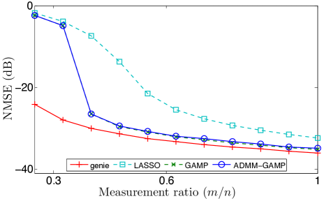
Figure 2: Average NMSE versus measurement rate $m/n$ when recovering a length $n=1000$ Bernoulli-Gaussian signal $\mathbf{x}$ from AWGN-corrupted measurements $\mathbf{y}=\mathbf{A}\mathbf{x}+\mathbf{e}$ under i.i.d. $\mathbf{A}$.

Note that the case of i.i.d. $\mathbf{A}$ is the “ideal” scenario for both AMP and GAMP. As discussed in the Introduction, their convergence in this case is guaranteed rigorously through state evolution analysis [23, 22, 24] as $m,n\rightarrow\infty$. In Figure 2, since $m$ and $n$ are sufficiently large, it is not surprising to see that GAMP performs well over all measurement ratios $m/n$. Furthermore, it is interesting to notice that GAMP outperforms LASSO and obtains NMSEs that are very close to that of the support-aware genie. Under such ideal $\mathbf{A}$, the proposed ADMM-GAMP method matches the performance of GAMP (since it minimizes the same objective) but does not offer any additional benefit.

The benefits of ADMM-GAMP become apparent in our second experiment, which uses non-i.i.d. matrices $\mathbf{A}$. In describing the experiment, we first recall that [25] established that the convergence of GAMP can be predicted by the peak-to-average ratio of the squared singular values,

$$\kappa(\mathbf{A})\triangleq\frac{\sigma_{1}^{2}(\mathbf{A})}{\sum_{i=1}^{r}\sigma_{i}^{2}(\mathbf{A})/r},$$ (81)

where $r=\min\{m,n\}$ and $\sigma_{i}(\mathbf{A})$ is the $i$-th largest singular value of $\mathbf{A}$. When this ratio $\kappa$ is sufficiently large, the algorithm will diverge. Thus, to test the robustness of ADMM-GAMP, we constructed a sequence of matrices $\mathbf{A}$ with varying $\kappa$, as follows. First, the left and right singular vectors of $\mathbf{A}$ were generated by drawing an $m\times n$ matrix with i.i.d. $\mathcal{N}(0,1/m)$ entries and taking its singular-value decomposition. Then, the singular values of $\mathbf{A}$ were chosen by setting the largest at $\sigma_{1}(\mathbf{A})=1$ and logarithmically spacing each successive singular value to attain the desired peak-to-average ratio $\kappa$.

As a function of $\kappa$, the NMSE performance of the various algorithms under test is illustrated in Figure 3 for the case of $m=600$ measurements. There it can be seen that, for larger values of $\kappa$, the NMSE performance of the original GAMP algorithm deteriorated, which was a result of the algorithm diverging. (Note that, in the plot, we capped the maximum NMSE to $0$ dB for visual clarity.) The figure also shows that the SwAMP method achieved low NMSE over a wider range of $\kappa$ ratios than the original GAMP method, but its performance also degraded for larger values of $\kappa$. The ADMM-GAMP method, however, converged over the entire range of $\kappa$ values, achieving NMSE performance relatively close to the support-aware genie.

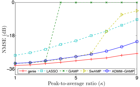
Figure 3: Average NMSE versus peak-to-average squared-singular-value ratio $\kappa(\mathbf{A})$ when recovering a length $n=1000$ Bernoulli-Gaussian signal $\mathbf{x}$ from $m=600$ AWGN-corrupted measurements $\mathbf{y}=\mathbf{A}\mathbf{x}+\mathbf{e}$. Note the superior performance of ADMM-GAMP relative to both the original GAMP and SwAMP, and the proximity of ADMM-GAMP to the support-aware genie.

In our third and final experiment, we recover $\mathbf{x}$ from “one-bit” measurements $\mathbf{y}=\mathrm{sgn}(\mathbf{A}\mathbf{x})$, where $\mathrm{sgn}$ is the sign function, as considered in, e.g., [53] and [40]. Here, we used $m=2000$ measurements and generated the matrices $\mathbf{A}$ as in our second experiment. Figure 4 shows the NMSE performance of the various algorithms under test. The results in the figure illustrate that the original GAMP method diverged for $\kappa\geq 2$. However, both SwAMP and ADMM-GAMP recovered the solution for the whole range of $\kappa$ without diverging, with ADMM-GAMP yielding slightly better NMSE (about $0.3$ dB better) at higher values of $\kappa$.

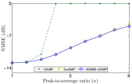
Figure 4: Average NMSE versus peak-to-average squared-singular-value ratio $\kappa(\mathbf{A})$ when recovering a length $n=1000$ Bernoulli-Gaussian signal $\mathbf{x}$ from $m=2000$ noiseless 1-bit measurements $\mathbf{y}=\mathrm{sgn}(\mathbf{A}\mathbf{x})$. Note the superior performance of ADMM-GAMP relative to the original GAMP and SwAMP.

Conclusions

Despite many promising results of AMP methods, the major stumbling block to more widespread use is their convergence and numerical stability. Although AMP techniques admit provable guarantees for i.i.d. $\mathbf{A}$, they can easily diverge for transforms that occur in many practical problems. While several methods have been proposed to improve the convergence, this paper provides a method with provable guarantees under arbitrary transforms. The method leverages well-established concepts of double-loop methods in belief propagation [32] as well as the classic ADMM method in optimization [9].

Nevertheless, there is still much work to be done. Most obviously, the proposed ADMM-GAMP method comes at a computational cost. Each iteration requires solving a (potentially large) least squares problem (49) that is not needed in the original AMP and GAMP algorithms. Similar to standard applications of ADMM, this minimization can likely be performed via conjugate gradient iterations, but its implementation requires further study. In any case, it is possible that ADMM-GAMP will be slower than other variants of GAMP. Indeed, our simulations suggest that other methods such as SwAMP or adaptively damped GAMP [28] may provide equally robust performance with less cost per iteration. One line of future work would thus be see to whether the proof techniques in this paper can be extended to address these algorithms as well.

The analysis in this paper might also be extended to other variants of AMP and GAMP. For example, it is conceivable that similar analysis could be applied to develop convergent approaches to the expectation-maximization (EM) GAMP developed in [54, 55, 56, 57, 41], turbo and hybrid GAMP methods in [58, 59] and applications in dictionary learning and matrix factorization [60, 61, 62].

Appendix A Proof of Theorem 1

Throughout this appendix, we use the shorthand notation for the gradient $h^{\prime}({\bm{\tau}})\triangleq\partial h({\bm{\tau}})/\partial{\bm{\tau}}\in{\mathbb{R}}^{p}$.

First we show, by induction, that ${\bm{\gamma}}^{k}\in\Gamma$ for all $k$. Recall that, by the hypothesis of the theorem, ${\bm{\gamma}}^{0}\in\Gamma$. Now suppose that ${\bm{\gamma}}^{k}\in\Gamma$. Then the updates in Algorithm 1 imply that

$$h^{\prime}({\bm{\tau}}^{k})=h^{\prime}(\mathbf{g}(\mathbf{b}^{k}))=h^{\prime}(\mathbf{g}(\widehat{\mathbf{b}}({\bm{\gamma}}^{k}))).$$

Then, by Assumption 1(c), $h^{\prime}({\bm{\tau}}^{k})\in\Gamma$. Since ${\bm{\gamma}}^{k}\in\Gamma$, $\theta^{k}\in(0,1]$, and $\Gamma$ is convex,

$${\bm{\gamma}}^{k\!+\!1}=(1-\theta^{k}){\bm{\gamma}}^{k}+\theta^{k}h^{\prime}({\bm{\tau}}^{k})\in\Gamma.$$

Thus, by induction, ${\bm{\gamma}}^{k}\in\Gamma$ for all $k$.

Next, we prove the decrementing property (27). First observe that since the restriction $\mathbf{b}\in B$ is a linear constraint, we can find a linear transform $\mathbf{B}$ and vector $\mathbf{b}_{0}$ such that $\mathbf{b}\in B$ if and only if $\mathbf{b}=\mathbf{B}\mathbf{x}+\mathbf{b}_{0}$ for some vector $\mathbf{x}$. It can be verified that we can reparameterize the functions $f(\cdot)$ and $\mathbf{g}(\cdot)$ around $\mathbf{x}$ and obtain the exact same recursions in Algorithm 1. Also, all the conditions in Assumptions 1 will hold for reparametrized functions as well. Thus, for the remainder of the proof we can ignore the linear constraints $B$, or alternatively view $B$ as the entire vector space.

Under this assumption, for any ${\bm{\gamma}}$, and any minimizer $\widehat{\mathbf{b}}({\bm{\gamma}})$ will be in the interior of $B$ and therefore,

$$\mathbf{0} = \frac{\partial J(\widehat{\mathbf{b}}({\bm{\gamma}}),{\bm{\gamma}})}{\partial\mathbf{b}}=f^{\prime}(\widehat{\mathbf{b}}({\bm{\gamma}}))+\sum_{\ell=1}^{L}g_{\ell}^{\prime}(\widehat{\mathbf{b}}({\bm{\gamma}}))\gamma_{\ell}$$ (82)

$$= f^{\prime}(\widehat{\mathbf{b}}({\bm{\gamma}}))+g^{\prime}(\widehat{\mathbf{b}}({\bm{\gamma}})){\bm{\gamma}},$$ (83)

where $f^{\prime}(\mathbf{b})$ is shorthand notation for the gradient $\partial f(\mathbf{b})/\partial\mathbf{b}$, $g_{\ell}^{\prime}(\mathbf{b})$ is shorthand for the gradient (with respect to $\mathbf{b}$) of the $\ell$th component of the vector-valued function $\mathbf{g}(\cdot)$, and where $g^{\prime}(\mathbf{b})=[g_{1}^{\prime}(\mathbf{b}),\dots,g_{L}^{\prime}(\mathbf{b})]$ is matrix-valued. Taking the gradient of (82) with respect to ${\bm{\gamma}}^{\text{\sf T}}$ yields the matrix

$$\mathbf{0} \stackrel{{\scriptstyle(a)}}{{=}} \frac{\partial f^{\prime}(\widehat{\mathbf{b}}({\bm{\gamma}}))}{\partial{\bm{\gamma}}^{\text{\sf T}}}+\sum_{\ell=1}^{L}\frac{\partial g_{\ell}^{\prime}(\widehat{\mathbf{b}}({\bm{\gamma}}))}{\partial{\bm{\gamma}}^{\text{\sf T}}}\gamma_{\ell}+g^{\prime}(\widehat{\mathbf{b}}({\bm{\gamma}}))$$ (84)

$$\stackrel{{\scriptstyle(b)}}{{=}} \left[\frac{\partial f^{\prime}(\widehat{\mathbf{b}}({\bm{\gamma}}))}{\partial\widehat{\mathbf{b}}^{\text{\sf T}}}+\sum_{\ell=1}^{L}\frac{\partial g_{\ell}^{\prime}(\widehat{\mathbf{b}}({\bm{\gamma}}))}{\partial\widehat{\mathbf{b}}^{\text{\sf T}}}\gamma_{\ell}\right]\frac{\partial\widehat{\mathbf{b}}({\bm{\gamma}})}{\partial{\bm{\gamma}}^{\text{\sf T}}}+g^{\prime}(\widehat{\mathbf{b}}({\bm{\gamma}}))$$

$$= \mathbf{H}({\bm{\gamma}})\frac{\partial\widehat{\mathbf{b}}({\bm{\gamma}})}{\partial{\bm{\gamma}}^{\text{\sf T}}}+g^{\prime}(\widehat{\mathbf{b}}({\bm{\gamma}})),$$

where (a) and (b) follow from the chain rule and $\mathbf{H}({\bm{\gamma}})$ is the Hessian from (25). Equation (84) then implies

$$\frac{\partial\widehat{\mathbf{b}}({\bm{\gamma}})}{\partial{\bm{\gamma}}^{\text{\sf T}}}=-\mathbf{H}({\bm{\gamma}})^{-1}g^{\prime}(\widehat{\mathbf{b}}({\bm{\gamma}})),$$ (85)

where Assumption 1(b) guarantees the existence of the inverse. The gradient of the objective with respect to ${\bm{\gamma}}^{\text{\sf T}}$ is then

$$\frac{\partial J(\widehat{\mathbf{b}}({\bm{\gamma}}))}{\partial{\bm{\gamma}}^{\text{\sf T}}} \stackrel{{\scriptstyle(a)}}{{=}} \left[f^{\prime}(\widehat{\mathbf{b}}({\bm{\gamma}}))+g^{\prime}(\widehat{\mathbf{b}}({\bm{\gamma}}))h^{\prime}({\bm{\tau}})\right]^{\text{\sf T}}\frac{\partial\widehat{\mathbf{b}}({\bm{\gamma}})}{\partial{\bm{\gamma}}^{\text{\sf T}}}$$ (86)

$$\stackrel{{\scriptstyle(b)}}{{=}} \big{(}h^{\prime}({\bm{\tau}})-{\bm{\gamma}}\big{)}^{\text{\sf T}}g^{\prime}(\widehat{\mathbf{b}}({\bm{\gamma}}))^{\text{\sf T}}\frac{\partial\widehat{\mathbf{b}}({\bm{\gamma}})}{\partial{\bm{\gamma}}^{\text{\sf T}}}$$

$$\stackrel{{\scriptstyle(c)}}{{=}} \big{(}{\bm{\gamma}}-h^{\prime}({\bm{\tau}})\big{)}^{\text{\sf T}}g^{\prime}(\widehat{\mathbf{b}}({\bm{\gamma}}))^{\text{\sf T}}\mathbf{H}({\bm{\gamma}})^{-1}g^{\prime}(\widehat{\mathbf{b}}({\bm{\gamma}})),\qquad$$

where (a) follows from (22) and the chain rule, (b) follows from (83), and (c) follows from (85).

Notice that the ${\bm{\gamma}}^{k}$ update in Algorithm 1 can be written as

$${\bm{\gamma}}^{k\!+\!1}-{\bm{\gamma}}^{k}=\big{(}h^{\prime}({\bm{\tau}}^{k})-{\bm{\gamma}}^{k}\big{)}\theta^{k}.$$

Taking an inner product of the above and (86) evaluated at ${\bm{\gamma}}={\bm{\gamma}}^{k}$, we get

$$\left[\frac{\partial J(\widehat{\mathbf{b}}({\bm{\gamma}}^{k}))}{\partial{\bm{\gamma}}^{\text{\sf T}}}\right]\left({\bm{\gamma}}^{k\!+\!1}-{\bm{\gamma}}^{k}\right)$$ (87)

$$= -\big{(}{\bm{\gamma}}^{k}-h^{\prime}({\bm{\tau}}^{k})\big{)}^{\text{\sf T}}g^{\prime}(\mathbf{b}^{k})^{\text{\sf T}}\mathbf{H}({\bm{\gamma}}^{k})^{-1}g^{\prime}(\mathbf{b}^{k})\big{(}{\bm{\gamma}}^{k}-h^{\prime}({\bm{\tau}}^{k})\big{)}\theta^{k}$$

$$\leq -\frac{\theta^{k}}{c_{2}}\big{\|}g^{\prime}(\mathbf{b}^{k})\big{(}{\bm{\gamma}}^{k}-h^{\prime}({\bm{\tau}}^{k})\big{)}\big{\|}^{2},$$

recalling that $\widehat{\mathbf{b}}(\gamma^{k})=\mathbf{b}^{k}$ and that $c_{2}$ was defined in Assumption 1(b). Therefore, the update of ${\bm{\gamma}}^{k}$ is in a descent direction on the objective $J(\widehat{\mathbf{b}}({\bm{\gamma}}))$. Hence, for a sufficiently small damping parameter $\theta^{k}$, we will have

$$J(\mathbf{b}^{k\!+\!1})-J(\mathbf{b}^{k})=J(\widehat{\mathbf{b}}({\bm{\gamma}}^{k\!+\!1}))-J(\widehat{\mathbf{b}}({\bm{\gamma}}^{k}))\leq 0,$$

which proves the decrementing property (27).

Appendix B Large Deviations View of MAP Estimation

For each $T>0$, let $\mathbf{x}^{t}(T),\mathbf{z}^{t}(T),\ldots$, be the output of the ADMM-GAMP algorithm with the MMSE estimation functions (51) and the scaled penalties (67). Next, we define several limits. For the mean vectors we define

$$\mathbf{x}^{t}=\lim_{T\rightarrow 0}\mathbf{x}^{t}(T),\quad\mathbf{z}^{t}=\lim_{T\rightarrow 0}\mathbf{z}^{t}(T),$$

for the dual vectors we define

$$\mathbf{q}^{t}=\lim_{T\rightarrow 0}T\mathbf{q}^{t}(T),\quad\mathbf{s}^{t}=\lim_{T\rightarrow 0}T\mathbf{s}^{t}(T),$$

and for the variance terms we define

$${\bm{\tau}}_{x}^{t} = \lim_{T\rightarrow 0}\frac{{\bm{\tau}}_{x}^{t}(T)}{T},{\bm{\tau}}_{z}^{t}=\lim_{T\rightarrow 0}\frac{{\bm{\tau}}_{z}^{t}(T)}{T},{\bm{\tau}}_{p}^{t}=\lim_{T\rightarrow 0}\frac{{\bm{\tau}}_{p}^{t}(T)}{T},\qquad$$ (88a)

$${\bm{\tau}}_{r}^{t} = \lim_{T\rightarrow 0}\frac{{\bm{\tau}}_{r}^{t}(T)}{T},{\bm{\tau}}_{s}^{t}=\lim_{T\rightarrow 0}T{\bm{\tau}}_{s}^{t}(T).$$ (88b)

We will assume that all of these limits exist. Note that some of terms are scaled by $T$ and others by $1/T$. These normalizations are important. It is easily checked that the scalings all cancel, so that the limiting values satisfy the recursions of Algorithm 3 with the limiting estimation functions

$$g_{x}(\mathbf{r},{\bm{\tau}}_{r}) \triangleq \lim_{T\rightarrow 0}g_{x}(\mathbf{r},{\bm{\tau}}_{r}(T);T)=\lim_{T\rightarrow 0}g_{x}(\mathbf{r},{\bm{\tau}}_{r}T;T),\qquad$$ (89a)

$$g_{z}(\mathbf{p},{\bm{\tau}}_{p}) \triangleq \lim_{T\rightarrow 0}g_{z}(\mathbf{p},{\bm{\tau}}_{p}(T);T)=\lim_{T\rightarrow 0}g_{z}(\mathbf{p},{\bm{\tau}}_{p}T;T),$$ (89b)

where $g_{x}(\mathbf{r},{\bm{\tau}}_{r}T;T)$ and $g_{z}(\mathbf{p},{\bm{\tau}}_{p}T;T)$ are the MMSE estimation functions (51) for the scaled penalties (67). Note that we have used the scalings in (88), which show ${\bm{\tau}}_{r}(T)\approx T{\bm{\tau}}_{r}$ and ${\bm{\tau}}_{p}(T)\approx{\bm{\tau}}_{p}T$ for small $T$. Now, the scaled function $g_{x}(\mathbf{r},{\bm{\tau}}_{r}T;T)$ is the expectation $\mathbb{E}(\mathbf{x}|T)$ with respect to the density

$$p(\mathbf{x}|\mathbf{r},{\bm{\tau}}_{r}T;T)\propto\exp\left[-\frac{f_{x}(\mathbf{x})}{T}-\frac{1}{2T}\|\mathbf{x}-\mathbf{r}\|^{2}_{{\bm{\tau}}_{r}}\right].$$

Laplace’s Principle [50] from large deviations theory shows that (under mild conditions) this density concentrates around its maxima, and thus the expectation with respect to this density converges to the minimum

$$\lim_{T\rightarrow 0}g_{x}(\mathbf{r},{\bm{\tau}}_{r}T;T)=\mathop{\mathrm{arg\,min}}_{\mathbf{x}}f_{x}(\mathbf{x})+\tfrac{1}{2}\|\mathbf{x}-\mathbf{r}\|^{2}_{{\bm{\tau}}_{r}},$$

which is exactly the minimization in the MAP estimation function (62). The limit of $g_{z}(\mathbf{p},{\bm{\tau}}_{p}/T;T)$ as $T\rightarrow 0$ is similar. We conclude that the limit of the ADMM-GAMP algorithm with MMSE estimation functions (51) and scaled densities (67) is exactly the ADMM-GAMP algorithm with the MAP estimation functions (62). In particular, for each $T$, the density over $x_{j}$ in (47) is given by

$$b_{x_{j}}^{t}(x_{j}|r_{j},\tau_{r_{j}}T)\propto\exp\left[-\frac{f_{x_{j}}(x_{j})}{T}-\frac{(x_{j}-r_{j}^{t})^{2}}{2T\tau_{r_{j}}^{t}}\right],$$ (90)

from which we can prove the limits in (68).

It remains to show that the LSL-BFE in (16) with the scaled functions (67) decomposes into the optimizations (56) and (71) as $T\rightarrow 0$. To this end, let $J(b_{x},b_{z};T)$ be the LSL-BFE (16) for the scaled penalties (67), which is given by

$$J(b_{x},b_{z};T) = D(b_{x}\|Z_{x,T}^{-1}\mathrm{e}^{-f_{x}/T})+D(b_{z}\|Z_{z,T}^{-1}\mathrm{e}^{-f_{z}/T})$$ (91)

$$\mbox{}+H(\mbox{var}(\mathbf{x}|b_{x}),\mbox{var}(\mathbf{z}|b_{z}))$$

$$= \frac{1}{T}\Big{[}\mathbb{E}(f_{x}(\mathbf{x})|b_{x})+\mathbb{E}(f_{z}(\mathbf{z})|b_{z})\Big{]}$$

$$\mbox{}+H(\mbox{var}(\mathbf{x}|b_{x}),\mbox{var}(\mathbf{z}|b_{z}))$$

$$\mbox{}-H(b_{x})-H(b_{z})+\text{const},$$

where $H(a)$ denotes the differential entropy of distribution $a$, $H({\bm{\tau}}_{x},{\bm{\tau}}_{z})$ is the entropy bound from (17), $Z_{x,T}\triangleq\int\mathrm{e}^{-f_{x}(\mathbf{x})/T}\mathrm{\,d}\mathbf{x}$, $Z_{z,T}\triangleq\int\mathrm{e}^{-f_{z}(\mathbf{z})/T}\mathrm{\,d}\mathbf{z}$, and the “const” in (91) is with respect to $b_{x}$ and $b_{z}$. Now, we know that, as $T\rightarrow 0$, the optimal densities $b_{x}$ and $b_{z}$ will concentrate around their maxima with variance $O(T)$. Thus, we can take a quadratic approximation around the maximum

$$\ln b_{x_{j}}(x_{j})\approx\frac{(x_{j}-\widehat{x}_{j})^{2}}{2T\tau_{x_{j}}}+\text{const},$$ (92)

where

$$\widehat{x}_{j}=\mathop{\mathrm{arg\,min}}_{x_{j}}-\ln b_{x_{j}}(x_{j}),\quad\frac{1}{\tau_{x_{j}}}=-T\frac{\partial^{2}\ln b_{x_{j}}(x_{j})}{\partial x_{j}^{2}},$$

with a similar approximation for $\ln b_{z_{i}}(z_{i})$. Under these approximations, $b_{x_{j}}(x_{j})$ and $b_{z_{i}}(z_{i})$ become approximately Gaussian, i.e.,

$$b_{x_{j}}(x_{j})\approx{\mathcal{N}}(\widehat{x}_{j},T\tau_{x_{j}}),\quad b_{z_{i}}(z_{i})\approx{\mathcal{N}}(\widehat{z}_{i},T\tau_{z_{i}}).$$ (93)

Using these Gaussian approximations, we can compute the expectations

$$\mathbb{E}(f_{x_{j}}(x_{j})|b_{x_{j}})=\int f_{x_{j}}(x)\mathcal{N}(x;\widehat{x}_{j},T\tau_{x_{j}})\mathrm{\,d}x$$ (94)

$$\stackrel{{\scriptstyle(a)}}{{=}} \int\sum_{k=0}^{\infty}\frac{(x-\widehat{x}_{j})^{k}f_{x_{j}}^{(k)}(\widehat{x}_{j})}{k!}\mathcal{N}(x;\widehat{x}_{j},T\tau_{x_{j}})\mathrm{\,d}x$$

$$\stackrel{{\scriptstyle(b)}}{{=}} \sum_{k=0}^{\infty}\frac{f_{x_{j}}^{(k)}(\widehat{x}_{j})}{k!}\int(x-\widehat{x}_{j})^{k}\mathcal{N}(x;\widehat{x}_{j},T\tau_{x_{j}})\mathrm{\,d}x$$ (95)

$$\stackrel{{\scriptstyle(c)}}{{=}} \sum_{l=0}^{\infty}\frac{f_{x_{j}}^{(2l)}(\widehat{x}_{j})}{(2l)!}(T\tau_{x_{j}})^{l}(2l-1)!!$$ (96)

$$\stackrel{{\scriptstyle(c)}}{{=}} \sum_{l=0}^{\infty}\frac{f_{x_{j}}^{(2l)}(\widehat{x}_{j})}{2^{l}l!}(T\tau_{x_{j}})^{l},$$ (97)

where (a) wrote $f_{x_{j}}(x)$ using a Taylor series about $x=\widehat{x}_{j}$; (b) assumed the exchange of limit and integral; (c) used the expression for the Gaussian central moments, which involves the double factorial $(2l-1)!!=(2l-1)(2l-3)(2l-5)\times\dots\times 1$; and (d) used the identity $(2l-1)!!=\frac{(2l)!}{2^{l}l!}$. Thus, for small $T$, we have

$$\mathbb{E}(f_{x_{j}}(x_{j})|b_{x_{j}}) \approx f_{x_{j}}(\widehat{x}_{j})+\frac{1}{2}T\tau_{x_{j}}f_{x_{j}}^{\prime\prime}(\widehat{x}_{j}),$$ (98a)

$$\mathbb{E}(f_{z_{i}}(z_{i})|b_{z_{i}}) \approx f_{z_{i}}(\widehat{z}_{i})+\frac{1}{2}T\tau_{z_{i}}f_{z_{i}}^{\prime\prime}(\widehat{z}_{i}).$$ (98b)

The differential entropies of these Gaussians (93) are

$$H(b_{x_{j}})=\frac{1}{2}\ln(2\pi eT\tau_{x_{j}}),\quad H(b_{z_{i}})=\frac{1}{2}\ln(2\pi eT\tau_{z_{i}}),$$ (99)

and the entropy term (17) is

$$H(\mbox{var}(\mathbf{x}|b_{x}),\mbox{var}(\mathbf{z}|b_{z}))=H(T{\bm{\tau}}_{x},T{\bm{\tau}}_{z})$$ (100)

$$= \frac{1}{2}\left[\sum_{i=1}^{m}\frac{\tau_{z_{i}}}{\tau_{p_{i}}}+\ln(2\pi T\tau_{p_{i}})\right],~{}{\bm{\tau}}_{p}\triangleq\mathbf{S}{\bm{\tau}}_{x}.$$

Substituting (98), (99) and (100) into (91), we obtain

$$J_{T}(b_{x},b_{z})=\frac{1}{T}J(\widehat{\mathbf{x}},\widehat{\mathbf{z}})+\frac{1}{2}J^{2}({\bm{\tau}}_{x},{\bm{\tau}}_{z},\widehat{\mathbf{x}},\widehat{\mathbf{z}})+\text{const},$$ (101)

where $J(\cdot)$ and $J^{2}(\cdot)$ are given in (56) and (VI-B). As $T\rightarrow 0$, the first term in (101) dominates, implying that the optimization of $(\widehat{\mathbf{x}},\widehat{\mathbf{z}})$ can be conducted independently of ${\bm{\tau}}_{x},{\bm{\tau}}_{z}$, as in (56). The subsequent optimization of $({\bm{\tau}}_{x},{\bm{\tau}}_{z})$ then follows, as given in (71).

Appendix C Proof of Theorems 2 and 3

We will just prove Theorem 2 since the proof of Theorem 3 is very similar. For the original constrained optimization (14), define the Lagrangian

$$L_{0}(b_{x},b_{z},\mathbf{s})\triangleq J(b_{x},b_{z})+\mathbf{s}^{\text{\sf T}}(\mathbb{E}(\mathbf{z}|b_{z})-\mathbf{A}\mathbb{E}(\mathbf{x}|b_{x})).$$ (102)

We need to show that any fixed points $(b_{x},b_{z},\mathbf{s})$ of ADMM-GAMP are critical points of this Lagrangian.

First observe that, any fixed point, ${\bm{\tau}}_{r}$ from line 22 of Algorithm 3 satisfies

$$\mathbf{1}./(2{\bm{\tau}}_{r})=\mathbf{1}./(2{\overline{\bm{\tau}}}_{r})=\frac{\partial H({\bm{\tau}}_{x},{\bm{\tau}}_{z})}{\partial{\bm{\tau}}_{x}},$$ (103)

where the last step follows from the construction of ${\overline{\bm{\tau}}}_{r}$ in (32). Similarly, at any fixed point of line 23,

$$\mathbf{1}./(2{\bm{\tau}}_{p})=\mathbf{1}./(2{\overline{\bm{\tau}}}_{p})=\frac{\partial H({\bm{\tau}}_{x},{\bm{\tau}}_{z})}{\partial{\bm{\tau}}_{z}}.$$ (104)

From (41b) and (41c), we see that any fixed point satisfies

$$\mathbb{E}(\mathbf{z}|b_{z})=\mathbf{A}\mathbf{v},\quad\mathbb{E}(\mathbf{x}|b_{x})=\mathbf{v}.$$ (105)

Thus, the constraint in (14) is satisfied, in that $\mathbb{E}(\mathbf{z}|b_{z})=\mathbf{A}\mathbb{E}(\mathbf{x}|b_{x})$. Furthermore, since $\mathbf{v}$ minimizes (49), we know that it zeros the gradient of the corresponding cost function:

$$\mathbf{0}=\mathbf{A}^{\text{\sf T}}\mathbf{D}_{{\bm{\tau}}_{p}}\big{(}\mathbb{E}(\mathbf{z}|b_{z})-\mathbf{A}\mathbf{v}+{\bm{\tau}}_{p}.\mathbf{s}\big{)}+\mathbf{D}_{{\bm{\tau}}_{r}}\big{(}\mathbb{E}(\mathbf{x}|b_{x})-\mathbf{v}+{\bm{\tau}}_{r}.\mathbf{q}\big{)},$$ (106)

where $\mathbf{D}_{{\bm{\tau}}}=\mathop{\mathrm{Diag}}(\mathbf{1}./{\bm{\tau}})$. Plugging (105) into the previous expression, we obtain

$$\mathbf{q}=-\mathbf{A}^{\text{\sf T}}\mathbf{s}.$$ (107)

Since $b_{x}$ minimizes the augmented Lagrangian in (41a), it zeros the corresponding gradient, i.e.,

$$\mathbf{0} = \frac{\partial}{\partial b_{x}}L(b_{x},b_{z},\mathbf{s},\mathbf{q},\mathbf{v};{\bm{\tau}}_{r},{\bm{\tau}}_{p})$$ (108)

$$\stackrel{{\scriptstyle(a)}}{{=}} \frac{\partial}{\partial b_{x}}\Bigl{[}J(b_{x},b_{z},{\bm{\tau}}_{r},{\bm{\tau}}_{p})+\mathbf{q}^{\text{\sf T}}\mathbb{E}(\mathbf{x}|b_{x})$$

$$\mbox{}+\frac{1}{2}\|\mathbb{E}(\mathbf{x}|b_{x})-\mathbf{v}\|^{2}_{{\bm{\tau}}_{r}}\Bigr{]}$$

$$\stackrel{{\scriptstyle(b)}}{{=}} \frac{\partial}{\partial b_{x}}\left[J(b_{x},b_{z},{\bm{\tau}}_{r},{\bm{\tau}}_{p})-\mathbf{q}^{\text{\sf T}}\mathbb{E}(\mathbf{x}|b_{x})\right]$$

$$\stackrel{{\scriptstyle(c)}}{{=}} \frac{\partial}{\partial b_{x}}\left[J(b_{x},b_{z},{\bm{\tau}}_{r},{\bm{\tau}}_{p})-\mathbf{s}^{\text{\sf T}}\mathbf{A}\mathbb{E}(\mathbf{x}|b_{x})\right]$$

$$\stackrel{{\scriptstyle(d)}}{{=}} \frac{\partial}{\partial b_{x}}\Bigg{[}J(b_{x},b_{z})-H\big{(}\mbox{var}(\mathbf{x}|b_{x}),{\bm{\tau}}_{z}\big{)}$$

$$\mbox{}+\left(\mathbf{1}./(2{\bm{\tau}}_{r})\right)^{\text{\sf T}}\mbox{var}(\mathbf{x}|b_{x})-\mathbf{s}^{\text{\sf T}}\mathbf{A}\mathbb{E}(\mathbf{x}|b_{x})\Bigg{]}$$

$$\stackrel{{\scriptstyle(e)}}{{=}} \frac{\partial}{\partial b_{x}}\left[J(b_{x},b_{z})-\mathbf{s}^{\text{\sf T}}\mathbf{A}\mathbb{E}(\mathbf{x}|b_{x})\right]$$

$$\stackrel{{\scriptstyle(f)}}{{=}} \frac{\partial}{\partial b_{x}}L_{0}(b_{x},b_{z},\mathbf{s}),$$

where (a) follows from substituting (40) and eliminating terms that do not depend on $b_{x}$, since their gradient equals zero; (b) follows from (105); (c) follows from (107); (d) follows from the definitions of the original and linearized LSL-BFEs in (16) and (31); (e) follows from the chain rule and the gradient in (103); and (f) follows from (102). A similar computation shows that

$$\frac{\partial}{\partial b_{z}}L_{0}(b_{x},b_{z},\mathbf{s})=\mathbf{0}.$$ (109)

Together, (108) and (109) show that $(b_{x},b_{z})$ are critical points of the Lagrangian $L_{0}(b_{x},b_{z},\mathbf{s})$ for the dual parameters $\mathbf{s}$. Since these densities also satisfy the constraint $\mathbb{E}(\mathbf{z}|b_{z})=\mathbf{A}\mathbb{E}(\mathbf{x}|b_{x})$, we conclude that $(b_{x},b_{z})$ are critical points of the constrained optimization (14).

Appendix D Proof of Lemma 1

For the MAP estimation functions (62), we know that

$$\widehat{x}_{j}=g_{x_{j}}(r_{j},\tau_{r_{j}})=\mathop{\mathrm{arg\,min}}_{x_{j}}f_{x_{j}}(x_{j})+\frac{1}{2\tau_{r_{j}}}(x_{j}-r_{j})^{2},$$

which implies that $x_{j}=\widehat{x}_{j}$ is a solution to $0=f_{x_{j}}^{\prime}(x_{j})+(x_{j}-r_{j})/\tau_{r_{j}}$, i.e., that

$$\widehat{x}_{j}=r_{j}-\tau_{r_{j}}f_{x_{j}}^{\prime}(\widehat{x}_{j}).$$

Taking the derivative with respect to $r_{j}$, we find

$$\frac{\partial\widehat{x}_{j}}{\partial r_{j}}=1-\tau_{r_{j}}f_{x_{j}}^{\prime\prime}(\widehat{x}_{j})\frac{\partial\widehat{x}_{j}}{\partial r_{j}},$$

which can be rearranged to form

$$\frac{\partial\widehat{x}_{j}}{\partial r_{j}}=g_{x_{j}}^{\prime}(r_{j},\tau_{r_{j}})=\frac{1}{1+f_{x_{j}}^{\prime\prime}(\widehat{x}_{j})\tau_{r_{j}}}.$$ (110)

Then, given the assumption in the lemma, (110) implies that

$$\frac{1}{1+B\tau_{r_{j}}}\leq g_{x_{j}}^{\prime}(r_{j},\tau_{r_{j}})\leq\frac{1}{1+A\tau_{r_{j}}}.$$

A similar bound can be obtained for $g_{z_{i}}^{\prime}(p_{i},\tau_{p_{i}})$, which proves (73) for any fixed ${\bm{\tau}}_{r}$ and ${\bm{\tau}}_{p}$.

The proof for MMSE estimation functions (51) uses a classic result of log-concave functions [63]. Since the functions $f_{x}$ and $f_{z}$ are separable, so are the estimation functions $g_{x}$ and $g_{z}$ (51), as established in (52). In particular, we can write

$$g_{x_{j}}(r_{j},\tau_{r_{j}})=\mathbb{E}(x_{j}|r_{j},\tau_{r_{j}}),\quad g_{z_{i}}(p_{i},\tau_{p_{i}})=\mathbb{E}(z_{i}|p_{i},\tau_{p_{i}}),$$

where the expectations are with respect to the densities

$$p(x_{j}|r_{j},\tau_{r_{j}}) \propto \exp\left[-f_{x_{j}}(x_{j})-\frac{(x_{j}-r_{j})^{2}}{2\tau_{r_{j}}}\right],$$ (111a)

$$p(z_{i}|p_{i},\tau_{p_{i}}) \propto \exp\left[-f_{z_{i}}(z_{i})-\frac{(z_{i}-p_{i})^{2}}{2\tau_{p_{i}}}\right].$$ (111b)

We then need to show that the condition (73) is satisfied for each of the functions $g_{x_{j}}$ and $g_{z_{i}}$. Below, we prove this for $g_{x_{j}}$, noting that the proof for $g_{z_{i}}$ is similar.

From (55), we know that the derivative of $g_{x_{j}}(r_{j},\tau_{r_{j}})$ with respect to $r_{j}$ is given by

$$g_{x_{j}}^{\prime}(r_{j},\tau_{r_{j}})=\frac{\tau_{x_{j}}}{\tau_{r_{j}}},\quad\tau_{x_{j}}=\mbox{var}(x_{j}|r_{j},\tau_{r_{j}}).$$ (112)

The variance here is with respect to the density (111a), which can be rewritten as

$$p(x_{j}|r_{j},\tau_{r_{j}})=\exp\left[-h(x_{j})\right]$$

for the potential function

$$h(x_{j})=f_{x_{j}}(x_{j})+\frac{(x_{j}-r_{j})^{2}}{2\tau_{r_{j}}},$$

which has second derivative

$$h^{\prime\prime}(x_{j})=f_{x_{j}}^{\prime\prime}(x_{j})+\frac{1}{\tau_{r_{j}}}.$$

By assumption (74), this derivative is bounded as

$$A+\frac{1}{\tau_{r_{j}}}\leq h^{\prime\prime}(x_{j})\leq B+\frac{1}{\tau_{r_{j}}}.$$

In particular, $h(x_{j})$ is strictly convex. From (112) and [63, Theorem 4.1], we have that

$$g_{x_{j}}^{\prime}(r_{j},\tau_{r_{j}})=\frac{\tau_{x_{j}}}{\tau_{r_{j}}}=\frac{\mbox{var}(x_{j}|r_{j},\tau_{r_{j}})}{\tau_{r_{j}}}$$ (113)

$$\leq\frac{1}{\tau_{r_{j}}}\mathbb{E}\left(\frac{1}{h^{\prime\prime}(x)}\right)\leq\frac{1}{A\tau_{r_{j}}+1}.$$

It is also shown in equation (4.13) of [63] that

$$g_{x_{j}}^{\prime}(r_{j},\tau_{r_{j}})=\frac{\tau_{x_{j}}}{\tau_{r_{j}}}=\frac{\mbox{var}(x_{j}|r_{j},\tau_{r_{j}})}{\tau_{r_{j}}}$$ (114)

$$\geq\frac{1}{\mathbb{E}(h^{\prime\prime}(x_{j}))\tau_{r_{j}}}\geq\frac{1}{B\tau_{r_{j}}+1}.$$

Thus, we conclude that

$$\frac{1}{1+B\tau_{r_{j}}}\leq g_{x_{j}}^{\prime}(r_{j},\tau_{r_{j}})\leq\frac{1}{1+A\tau_{r_{j}}},$$

which proves (73).

Appendix E Proof of Theorem 4

We find it easier to analyze the algorithm after the variables are combined and scaled as

$${\bm{\tau}}\triangleq\left[\begin{array}[]{c}{\bm{\tau}}_{r}\\ {\bm{\tau}}_{p}\end{array}\right],\quad\mathbf{D}\triangleq\mathop{\mathrm{Diag}}(\mathbf{1}./{\bm{\tau}}),$$ (115)

and

$$\mathbf{w}\triangleq\mathbf{D}^{1/2}\left[\begin{array}[]{c}\mathbf{x}\\ \mathbf{z}\end{array}\right],~{}\mathbf{u}\triangleq\mathbf{D}^{-1/2}\left[\begin{array}[]{c}\mathbf{q}\\ \mathbf{s}\end{array}\right],~{}\mathbf{B}\triangleq\mathbf{D}^{1/2}\left[\begin{array}[]{c}\mathbf{I}\\ \mathbf{A}\end{array}\right].$$ (116)

Also, we define

$$g(\mathbf{w},{\bm{\tau}})\triangleq\left[\begin{array}[]{c}g_{x}(\mathbf{x},{\bm{\tau}}_{r})\\ g_{z}(\mathbf{z},{\bm{\tau}}_{p})\end{array}\right],$$ (117)

and henceforth suppress the dependence on ${\bm{\tau}}$ in the notation since ${\bm{\tau}}$ is constant in this analysis. The mean update steps in Algorithm 3 then become

$$\mathbf{w}^{t\!+\!1} = \mathbf{D}^{1/2}g(\mathbf{D}^{-1/2}(\mathbf{B}\mathbf{v}^{t}-\mathbf{u}^{t}))$$ (118a)

$$\mathbf{u}^{t\!+\!1} = \mathbf{u}^{t}+\mathbf{w}^{t\!+\!1}-\mathbf{B}\mathbf{v}^{t}$$ (118b)

$$\mathbf{v}^{t\!+\!1} = \mathop{\mathrm{arg\,min}}_{\mathbf{v}}\|\mathbf{w}^{t\!+\!1}+\mathbf{u}^{t\!+\!1}-\mathbf{B}\mathbf{v}\|^{2},$$ (118c)

where the result of (118c) can be written explicitly as

$$\mathbf{v}^{t}=(\mathbf{B}^{\text{\sf T}}\mathbf{B})^{-1}\mathbf{B}^{\text{\sf T}}(\mathbf{w}^{t}+\mathbf{u}^{t}).$$ (119)

Let us define

$$\mathbf{P}\triangleq\mathbf{B}(\mathbf{B}^{\text{\sf T}}\mathbf{B})^{-1}\mathbf{B}^{\text{\sf T}},\quad\mathbf{P}^{\perp}\triangleq\mathbf{I}-\mathbf{P},$$ (120)

where $\mathbf{P}$ is an orthogonal projector operator onto the column space of $\mathbf{B}$ and $\mathbf{P}^{\perp}$ is the projection onto its orthogonal complement. Noting that $\mathbf{B}\mathbf{v}^{t}=\mathbf{P}(\mathbf{w}^{t}+\mathbf{u}^{t})$, (118a) reduces to

$$\mathbf{w}^{t\!+\!1} = \mathbf{D}^{1/2}g\left(\mathbf{D}^{-1/2}(\mathbf{P}\big{(}\mathbf{w}^{t}+\mathbf{u}^{t})-\mathbf{u}^{t}\big{)}\right)$$ (121)

$$= \mathbf{D}^{1/2}g\left(\mathbf{D}^{-1/2}(\mathbf{P}\mathbf{w}^{t}-\mathbf{P}^{\perp}\mathbf{u}^{t})\right)$$

$$= \tilde{g}(\mathbf{P}\mathbf{w}^{t}-\mathbf{P}^{\perp}\mathbf{u}^{t}),$$

where

$$\tilde{g}(\mathbf{w})\triangleq\mathbf{D}^{1/2}g(\mathbf{D}^{-1/2}\mathbf{w}).$$ (122)

Also, since $\mathbf{P}^{\perp}\mathbf{B}=\mathbf{0}$, (118b) implies that

$$\mathbf{P}^{\perp}\mathbf{u}^{t\!+\!1} = \mathbf{P}^{\perp}\mathbf{u}^{t}+\mathbf{P}^{\perp}\mathbf{w}^{t\!+\!1}$$ (123)

$$= \mathbf{P}^{\perp}\mathbf{u}^{t}+\mathbf{P}^{\perp}\tilde{g}(\mathbf{P}\mathbf{w}^{t}-\mathbf{P}^{\perp}\mathbf{u}^{t}).$$

Now define the state vector

$${\bm{\theta}}^{t}\triangleq\left[\begin{array}[]{c}\mathbf{P}\mathbf{w}^{t}\\ \mathbf{P}^{\perp}\mathbf{u}^{t}\end{array}\right].$$ (124)

Since $\mathbf{P}^{2}=\mathbf{P}$ and $(\mathbf{P}^{\perp})^{2}=\mathbf{P}^{\perp}$,

$$\left[\begin{array}[]{cc}\mathbf{P}&-\mathbf{P}^{\perp}\end{array}\right]{\bm{\theta}}^{t}=\mathbf{P}\mathbf{w}^{t}-\mathbf{P}^{\perp}\mathbf{u}^{t}.$$

Therefore, from (121) and (123), respectively, we have that

$$\mathbf{P}\mathbf{w}^{t\!+\!1} = \mathbf{P}\tilde{g}\big{(}\left[\begin{array}[]{cc}\mathbf{P}&-\mathbf{P}^{\perp}\end{array}\right]{\bm{\theta}}^{t}\big{)},$$ (126)

$$\mathbf{P}^{\perp}\mathbf{u}^{t\!+\!1} = \mathbf{P}^{\perp}\mathbf{u}^{t}+\mathbf{P}^{\perp}\tilde{g}\big{(}\left[\begin{array}[]{cc}\mathbf{P}&-\mathbf{P}^{\perp}\end{array}\right]{\bm{\theta}}^{t}\big{)}.$$ (128)

From (124), (126), and (128), we see that the mean update steps in Algorithm 3 are characterized by the recursive system

$${\bm{\theta}}^{t\!+\!1}=f({\bm{\theta}}^{t})$$ (129)

for

$$f({\bm{\theta}})\triangleq\left[\begin{array}[]{c}\mathbf{P}\\ \mathbf{P}^{\perp}\end{array}\right]\tilde{g}\big{(}\left[\begin{array}[]{cc}\mathbf{P}&-\mathbf{P}^{\perp}\end{array}\right]{\bm{\theta}}\big{)}+\left[\begin{array}[]{cc}\mathbf{0}&\mathbf{0}\\ \mathbf{0}&\mathbf{P}^{\perp}\end{array}\right]{\bm{\theta}}.$$ (130)

The following is a standard contraction mapping result [64]: if $f$ has a continuous Jacobian $f^{\prime}$ whose spectral norm is less than one, i.e., $\exists\epsilon>0\text{~{}s.t.~{}}\|f^{\prime}({\bm{\theta}})\|<1-\epsilon~{}\forall{\bm{\theta}}$, then the system (129) converges to a unique fixed point, ${\bm{\theta}}^{*}$, with a linear convergence rate, i.e.,

$$\exists C>0\text{~{}s.t.~{}}\|{\bm{\theta}}^{t}-{\bm{\theta}}^{*}\|\leq C(1-\epsilon)^{t}.$$

So, our proof will be complete if we can show that the Jacobian of $f$ from (130) is indeed a contraction.

First observe that, from the definition of $g(\mathbf{w})$ in (117), and the separability and boundedness assumptions in Assumption 2, the Jacobian of $g(\mathbf{w})$ at any $\mathbf{w}$ is diagonal and bounded:

$$\exists\epsilon\in(0,0.5]\text{~{}s.t.~{}}g^{\prime}(\mathbf{w})=\mathop{\mathrm{Diag}}(\mathbf{d})\text{~{}and~{}}\epsilon\leq d_{k}\leq 1-\epsilon~{}\forall k.$$

Since $\mathbf{D}=\mathop{\mathrm{Diag}}(\mathbf{1}./{\bm{\tau}})$ is also diagonal, the Jacobian of $\tilde{g}(\mathbf{w})$ in (122) is given by

$$\tilde{g}^{\prime}(\mathbf{w})=\mathbf{D}^{-1/2}\mathop{\mathrm{Diag}}(\mathbf{d})\mathbf{D}^{1/2}=\mathop{\mathrm{Diag}}(\mathbf{d}),$$

and hence

$$\epsilon\mathbf{I}\leq\tilde{g}^{\prime}(\mathbf{w})\leq(1-\epsilon)\mathbf{I}$$ (131)

for all $\mathbf{w}$. Now, the Jacobian of $f({\bm{\theta}})$ in (130) is given by

$$f^{\prime}({\bm{\theta}})=\left[\begin{array}[]{c}\mathbf{P}\\ \mathbf{P}^{\perp}\end{array}\right]\tilde{g}^{\prime}(\mathbf{w})\left[\begin{array}[]{cc}\mathbf{P}&-\mathbf{P}^{\perp}\end{array}\right]+\left[\begin{array}[]{cc}\mathbf{0}&\mathbf{0}\\ \mathbf{0}&\mathbf{P}^{\perp}\end{array}\right].$$ (132)

Hence, if we define

$$\mathbf{J}({\bm{\theta}})\triangleq f^{\prime}({\bm{\theta}})\left[\begin{array}[]{cc}\mathbf{I}&\mathbf{0}\\ \mathbf{0}&-\mathbf{I}\end{array}\right],$$ (133)

then $\|f^{\prime}({\bm{\theta}})\|=\|\mathbf{J}({\bm{\theta}})\|$ so $f^{\prime}({\bm{\theta}})$ is a contraction if and only if $\mathbf{J}({\bm{\theta}})$ is. Therefore, it suffices to prove that $\mathbf{J}({\bm{\theta}})$ is a contraction. Combining (132) and (133), we obtain

$$\mathbf{J}({\bm{\theta}})=\mathbf{U}^{\text{\sf T}}\tilde{g}^{\prime}(\mathbf{w})\mathbf{U}-\left[\begin{array}[]{cc}\mathbf{0}&\mathbf{0}\\ \mathbf{0}&\mathbf{P}^{\perp}\end{array}\right],$$ (134)

where $\mathbf{w}=\left[\begin{array}[]{cc}\mathbf{P}&\mathbf{P}^{\perp}\end{array}\right]{\bm{\theta}}$, and

$$\mathbf{U}=\left[\begin{array}[]{cc}\mathbf{P}&\mathbf{P}^{\perp}\end{array}\right].$$ (135)

Since $\mathbf{P}$ is an orthogonal projection and $\mathbf{P}^{\perp}$ is the projection onto the orthogonal complement, $\mathbf{U}$ is an isometry. That is,

$$\mathbf{U}\mathbf{U}^{\text{\sf T}}=\mathbf{P}+\mathbf{P}^{\perp}=\mathbf{I},$$ (136)

and hence $\mathbf{U}^{\text{\sf T}}\mathbf{U}\leq\mathbf{I}$. Therefore, from (134) and (131),

$$\mathbf{J}({\bm{\theta}})\leq\mathbf{U}^{\text{\sf T}}\tilde{g}^{\prime}(\mathbf{w})\mathbf{U}\leq(1-\epsilon)\mathbf{U}^{\text{\sf T}}\mathbf{U}\leq(1-\epsilon)\mathbf{I}.$$ (137)

For the lower bound, observe that

$$\mathbf{J}({\bm{\theta}}) \stackrel{{\scriptstyle(a)}}{{=}} \mathbf{U}^{\text{\sf T}}\tilde{g}^{\prime}(\mathbf{w})\mathbf{U}-\left[\begin{array}[]{cc}\mathbf{0}&\mathbf{0}\\ \mathbf{0}&\mathbf{P}^{\perp}\end{array}\right]$$ (140)

$$\stackrel{{\scriptstyle(b)}}{{\geq}} \epsilon\mathbf{U}^{\text{\sf T}}\mathbf{U}-\left[\begin{array}[]{cc}\mathbf{0}&\mathbf{0}\\ \mathbf{0}&\mathbf{P}^{\perp}\end{array}\right]$$ (143)

$$\stackrel{{\scriptstyle(c)}}{{=}} \left[\begin{array}[]{cc}\epsilon\mathbf{P}&\mathbf{0}\\ \mathbf{0}&(\epsilon-1)\mathbf{P}^{\perp}\end{array}\right]$$ (146)

$$\stackrel{{\scriptstyle(d)}}{{=}} \left[\begin{array}[]{cc}(\epsilon-1)\mathbf{I}&\mathbf{0}\\ \mathbf{0}&(\epsilon-1)\mathbf{I}\end{array}\right]+\left[\begin{array}[]{cc}\mathbf{I}-\epsilon\mathbf{P}^{\perp}&\mathbf{0}\\ \mathbf{0}&(1-\epsilon)\mathbf{P}\end{array}\right]$$ (151)

$$\geq (\epsilon-1)\mathbf{I},$$ (152)

where step (a) follows from (134); (b) follows from (131); (c) follows from the definition of $\mathbf{U}$ in (135) and the fact that $\mathbf{P}$ and $\mathbf{P}^{\perp}$ are orthogonal projections; (d) follows from the definition of $\mathbf{P}^{\perp}$ in (120); and (140) follows because the eigenvalues of $\mathbf{P}^{\perp}$ and $\mathbf{P}$ are in the interval $[0,1]$ and because $\epsilon\in(0,0.5]$. Together (137) and (140) show that

$$\|f^{\prime}({\bm{\theta}})\|=\|\mathbf{J}({\bm{\theta}})\|\leq 1-\epsilon.$$

Hence the $f^{\prime}({\bm{\theta}})$ is a contraction and the ADMM-GAMP algorithm converges linearly at rate $1-\epsilon$.

Appendix F Proof of Theorem 5

We need to prove that the conditions of Assumption 1 are satisfied. Property (a) is satisfied since Theorem 4 shows that the constrained linearized LSL-BFE optimization (36) has a unique minima for any $({\bm{\tau}}_{r},{\bm{\tau}}_{p})>0$.

We next construct the set $\Gamma$. From the proof of Lemma 1, we know that when ${\bm{\tau}}_{x}=\mbox{var}(\mathbf{x}|\mathbf{r},{\bm{\tau}}_{r})$ and ${\bm{\tau}}_{z}=\mbox{var}(\mathbf{z}|\mathbf{p},{\bm{\tau}}_{p})$,

$${\bm{\tau}}_{x}\in\left[\frac{A{\bm{\tau}}_{r}}{A+{\bm{\tau}}_{r}},\frac{B{\bm{\tau}}_{r}}{B+{\bm{\tau}}_{r}}\right],$$ (153)

$${\bm{\tau}}_{z}\in\left[\frac{A{\bm{\tau}}_{p}}{A+{\bm{\tau}}_{p}},\frac{B{\bm{\tau}}_{p}}{B+{\bm{\tau}}_{p}}\right],$$ (154)

Hence

$${\bm{\tau}}_{s}\triangleq\left(1-\frac{{\bm{\tau}}_{z}}{{\bm{\tau}}_{p}}\right)\frac{1}{{\bm{\tau}}_{p}}\in\left[\frac{1}{B+{\bm{\tau}}_{p}},\frac{1}{A+{\bm{\tau}}_{p}}\right].$$ (155)

Now consider a set $\Gamma$ of the form

$$\Gamma=\left\{({\bm{\tau}}_{r},{\bm{\tau}}_{p})~{}\mid~{}{\bm{\tau}}_{r}\in[a_{r},b_{r}],\quad{\bm{\tau}}_{p}\in[a_{p},b_{p}]\right\}.$$ (156)

In order that $\Gamma$ satisfies Assumption 1(c), we need to find bounds $a_{r},b_{r},a_{p},b_{p}$, such that if $({\bm{\tau}}_{r},{\bm{\tau}}_{p})\in\Gamma$, then $({\overline{\bm{\tau}}}_{r},{\overline{\bm{\tau}}}_{p})\in\Gamma$ where $({\overline{\bm{\tau}}}_{r},{\overline{\bm{\tau}}}_{p})$ are given in (35).

To this end, first observe that (153) shows that ${\bm{\tau}}_{x}\leq 1/B$, so ${\overline{\bm{\tau}}}_{p}=\mathbf{S}{\bm{\tau}}_{x}\leq b_{p}$ for some $b_{p}$. If ${\bm{\tau}}_{p}\leq b_{p}$, (155) shows that ${\bm{\tau}}_{s}\in[1/B,1/(A+b_{p})]$. Therefore, using the boundedness assumptions on $\mathbf{S}$, ${\overline{\bm{\tau}}}_{r}=\mathbf{1}./(\mathbf{S}^{\text{\sf T}}{\bm{\tau}}_{s})\in[a_{r},b_{r}]$ for some lower and upper bounds $a_{r}$ and $b_{r}$. Finally, if ${\bm{\tau}}_{r}\geq a_{r}$, ${\bm{\tau}}_{x}\geq Aa_{r}/(A+a_{r})$ and hence ${\overline{\bm{\tau}}}_{p}=\mathbf{S}{\bm{\tau}}_{x}\geq a_{p}$ for some $a_{p}$. We conclude that we can find bounds $a_{r},b_{r},a_{p},b_{p}$, such that if $({\bm{\tau}}_{r},{\bm{\tau}}_{p})\in\Gamma$, then $({\overline{\bm{\tau}}}_{r},{\overline{\bm{\tau}}}_{p})\in\Gamma$, and $\Gamma$ is a compact, convex set satisfying Assumption 1(c).

Finally, we need to show the convexity assumption in Assumption 1(b). The linearized LSL-BFE in (31) is separable, so we only need to consider the convexity of one of the terms. To this consider a prototypical term of the form

$$J(b)=D(b\|\mathrm{e}^{-f_{x}})+\frac{1}{2\tau_{r}}\mbox{var}(x|b),$$ (157)

where $b(x)$ is some density over a scalar variable $x$ and $f_{x}(x)$ is a convex penalty function. The Hessian of $J(b)$ is a quadratic form that takes perturbations $v_{1}(x)$ and $v_{2}(x)$ to the density $b(x)$ and returns a scalar. We will denote this Hessian by $J^{\prime\prime}(b)(v_{1},v_{2})$. Differentiating (157) we obtain that

$$J^{\prime\prime}(b)(v,v)=\int\frac{v(x)^{2}}{b(x)}\mathrm{\,d}x-\frac{1}{\tau_{r}}\left(\int v(x)x\mathrm{\,d}x\right)^{2}.$$ (158)

We need to show that this is positive. For any $v(x)$, let $u(x)=v(x)/b(x)$ so that $v(x)=u(x)b(x)$. Since a perturbation to the density $b(x)$ must satisfy $\int v(x)\mathrm{\,d}x=0$, we have that

$$\mathbb{E}(u(x)|b)=\int u(x)b(x)\mathrm{\,d}x=0.$$

Also, $J^{\prime\prime}(b)(v,v)$ above can be written as

$$J^{\prime\prime}(b)(v,v) \stackrel{{\scriptstyle(a)}}{{=}} \mathbb{E}(u(x)^{2}|b)-\frac{1}{\tau_{r}}\mathbb{E}(u(x)x|b)$$ (159)

$$\stackrel{{\scriptstyle(b)}}{{=}} \mbox{var}(u(x)|b)-\frac{1}{\tau_{r}}\mathbb{E}^{2}(u(x)(x-\mu_{x})|b)$$

$$\stackrel{{\scriptstyle(c)}}{{\geq}} \mbox{var}(u(x)|b)\left[1-\frac{\tau_{x}}{\tau_{r}}\right],$$

where (a) follows from substituting $v(x)=u(x)b(x)$ into (158); in (b) we have used the notation $\mu_{x}=\mathbb{E}(x|b)$ and the fact that $\mathbb{E}(u(x)|b)=0$; and (c) follows from the Cauchy-Schwartz inequality with the notation $\tau_{x}=\mbox{var}(x|b)$. Now, using (153), we see that when $({\bm{\tau}}_{r},{\bm{\tau}}_{p})\in\Gamma$, we have the lower bound,

$$1-\frac{\tau_{x}}{\tau_{r}}\geq 1-\frac{B}{B+a_{r}}\geq\frac{a_{r}}{B+a_{r}}>0.$$

We conclude that there exists an $\epsilon$ such that

$$J^{\prime\prime}(b)\geq\epsilon\mathbf{I},$$

at any minima $b=\widehat{b}$ to the linearized LSL-BFE when $({\bm{\tau}}_{r},{\bm{\tau}}_{p})\in\Gamma$. This proves Assumption 1(b). The uniform boundedness of all the other derivatives follows from the fact that all the terms are twice differentiable and the set $\Gamma$ is compact.

Thus, all the conditions of Assumption 1 and the theorem follows from Theorem 1.

Appendix G Proof of Theorem 6

We begin with proving part (a). We use induction. Suppose that (a) is satisfied for some $t$. Since $\mathbf{q}^{0}$, $\mathbf{x}^{0}$, and $\mathbf{v}^{0}$ are fixed points, we have from line 10 of Algorithm 3 that $\mathbf{x}^{0}=\mathbf{v}^{0}$. Then, since $\mathbf{x}^{0}$ is a fixed point, we have from lines 7 and 9 and equation (62) that

$$\mathbf{x}^{0}=g_{x}(\mathbf{r}^{0},{\bm{\tau}}_{r}^{0})=\mathop{\mathrm{arg\,min}}_{\mathbf{x}}f_{x}(\mathbf{x})+\frac{1}{2}\|\mathbf{x}-\mathbf{v}^{0}+{\bm{\tau}}_{r}^{0}.\mathbf{q}^{0}\|_{{\bm{\tau}}_{r}^{0}}^{2}.$$

Therefore, $\mathbf{x}=\mathbf{x}^{0}$ is the unique solution to

$$\mathbf{0}=f_{x}^{\prime}(\mathbf{x})+\mathop{\mathrm{Diag}}(\mathbf{1}./(2{\bm{\tau}}_{r}^{0}))(\mathbf{x}-\mathbf{x}^{0})+\mathbf{q}^{0},$$

which implies

$$f_{x}^{\prime}(\mathbf{x}^{0})=-\mathbf{q}^{0}.$$ (160)

By the induction hypothesis (a), $\mathbf{x}^{t}=\mathbf{x}^{0}$ and $\mathbf{q}^{t}=\mathbf{q}^{0}$. Since $\mathbf{x}^{t\!+\!1}=g_{x}(\mathbf{r}^{t},{\bm{\tau}}_{r}^{t})$, we have $\mathbf{x}=\mathbf{x}^{t\!+\!1}$ is the unique solution to

$$\mathbf{0} = f^{\prime}(\mathbf{x})+\mathop{\mathrm{Diag}}(\mathbf{1}./(2{\bm{\tau}}_{r}^{t}))(\mathbf{x}-\mathbf{r}^{t})$$ (161)

$$= f^{\prime}(\mathbf{x})+\mathop{\mathrm{Diag}}(\mathbf{1}./(2{\bm{\tau}}_{r}^{t}))(\mathbf{x}-\mathbf{x}^{0})+\mathbf{q}^{0},$$ (162)

where we have used the fact that

$$\mathbf{r}^{t}=\mathbf{x}^{t}+{\bm{\tau}}_{r}^{t}.\mathbf{q}^{t}=\mathbf{x}^{0}+{\bm{\tau}}_{r}^{t}.\mathbf{q}^{0}.$$

From (160), $\mathbf{x}=\mathbf{x}^{0}$ is also a solution to (161). Therefore, $\mathbf{x}^{t\!+\!1}=\mathbf{x}^{0}$. Similarly, if $\mathbf{s}^{t}=\mathbf{s}^{0}$ and $\mathbf{z}^{t}=\mathbf{z}^{0}$, then $\mathbf{z}^{t\!+\!1}=\mathbf{z}^{0}$. From (49), $\mathbf{v}^{t\!+\!1}=\mathbf{v}^{0}$. We conclude that if (a) is satisfied for some $t$, it is satisfied for $t\!+\!1$. So part (a) follows by induction.

To prove part (b), we leverage the convergence result from [65]. Using our earlier result (110), we have that

$$\tau_{x_{j}}^{t\!+\!1}=\tau_{r_{j}}^{t}g_{x_{j}}^{\prime}(r_{j}^{t},\tau_{r_{j}}^{t})=\frac{\tau_{r_{j}}^{t}}{1+f_{x_{j}}^{\prime\prime}(x_{j}^{t\!+\!1})\tau_{r_{j}}^{t}}.$$

Rewriting this in vector form and using the updates in Algorithm 3 with $\theta^{t}=1$, we obtain that

$$\mathbf{1}./{\bm{\tau}}_{x}^{t\!+\!1} = \mathbf{1}./{\bm{\tau}}_{r}^{t}+f_{x}^{\prime\prime}(\mathbf{x}^{t\!+\!1})=\mathbf{S}^{\text{\sf T}}{\bm{\tau}}_{s}^{t}+f_{x}^{\prime\prime}(\mathbf{x}^{t\!+\!1})$$ (163)

$$= \mathbf{S}^{\text{\sf T}}{\bm{\tau}}_{s}^{t}+{\bm{\xi}}_{x},\quad{\bm{\xi}}_{x}\triangleq f_{x}^{\prime\prime}(\mathbf{x}^{t\!+\!1})>\mathbf{0}$$

where $f_{x}^{\prime\prime}(\mathbf{x})=[f_{x_{1}}^{\prime\prime}(x_{1}),\dots,f_{x_{n}}^{\prime\prime}(x_{n})]^{\text{\sf T}}$ and where ${\bm{\xi}}_{x}$ is positive due to the convexity assumption and invariant to $t$ due to part (a). Similarly, for the output estimation function $g_{z}$,

$${\bm{\tau}}_{z}^{t\!+\!1}={\bm{\tau}}_{p}^{t}.g_{z}^{\prime}(\mathbf{p}^{t},{\bm{\tau}}_{p}^{t})={\bm{\tau}}_{p}^{t}./(\mathbf{1}+f_{z}^{\prime\prime}(\mathbf{z}^{t\!+\!1}).{\bm{\tau}}_{p}^{t}).$$

Therefore, from the modified update of ${\bm{\tau}}_{s}^{t\!+\!1}$ in (76),

$${\bm{\tau}}_{s}^{t\!+\!1}=f_{z}^{\prime\prime}(\mathbf{z}^{t\!+\!1})./(\mathbf{1}+f_{z}^{\prime\prime}(\mathbf{z}^{t\!+\!1}).{\bm{\tau}}_{p}^{t}),$$

or equivalently,

$$\mathbf{1}./{\bm{\tau}}_{s}^{t\!+\!1} = {\bm{\tau}}_{p}^{t}+\mathbf{1}./f_{z}^{\prime\prime}(\mathbf{z}^{t\!+\!1})=\mathbf{S}{\bm{\tau}}_{x}^{t}+{\bm{\xi}}_{z}$$ (164)

$${\bm{\xi}}_{z} \triangleq \mathbf{1}./f_{z}^{\prime\prime}(\mathbf{z}^{t\!+\!1}).$$ (165)

Now define the maps,

$$\Phi_{s}({\bm{\tau}}_{x}) := \mathbf{1}./\big{(}\mathbf{S}{\bm{\tau}}_{x}+{\bm{\xi}}_{z}\big{)}$$

$$\Phi_{x}({\bm{\tau}}_{s}) := \mathbf{1}./\big{(}\mathbf{S}^{\text{\sf T}}{\bm{\tau}}_{s}+{\bm{\xi}}_{x}\big{)}$$

so that the updates (164) and (163) can be written as

$${\bm{\tau}}_{s}^{t}=\Phi_{s}({\bm{\tau}}_{x}^{t\!-\!1}),\quad{\bm{\tau}}_{x}^{t\!+\!1}=\Phi_{x}({\bm{\tau}}^{t}_{s}).$$

Note that, due to part (a), ${\bm{\xi}}_{x}$ and ${\bm{\xi}}_{z}$ in (163) and (164), do not change with $t$. It is easy to check that, for any $\mathbf{S}>0$,

1. $\Phi_{s}({\bm{\tau}}_{x})>0$,

2. ${\bm{\tau}}_{x}\geq{\bm{\tau}}_{x}^{\prime}\Rightarrow\Phi_{s}({\bm{\tau}}_{x})\leq\Phi_{s}({\bm{\tau}}_{x}^{\prime})$, and

3. For all $\alpha>1$, $\Phi_{s}(\alpha{\bm{\tau}}_{x})>(1/\alpha)\Phi_{s}({\bm{\tau}}_{x})$.

with the analogous properties being satisfied by $\Phi_{x}({\bm{\tau}}_{s})$. Now let $\Phi:=\Phi_{x}\circ\Phi_{s}$ be the composition of the two functions so that ${\bm{\tau}}^{t\!+\!1}_{x}=\Phi({\bm{\tau}}_{x}^{t\!-\!1})$. Then, $\Phi$ satisfies the three properties:

1. $\Phi({\bm{\tau}}_{x})>0$,

2. ${\bm{\tau}}_{x}\geq{\bm{\tau}}_{x}^{\prime}\Rightarrow\Phi({\bm{\tau}}_{x})\geq\Phi({\bm{\tau}}_{x}^{\prime})$, and

3. For all $\alpha>1$, $\Phi(\alpha{\bm{\tau}}_{x})<\alpha\Phi({\bm{\tau}}_{x})$.

Also, for any ${\bm{\tau}}_{s}\geq 0$, we have $\Phi_{x}({\bm{\tau}}_{s})\leq\mathbf{1}./{\bm{\xi}}_{x}$, and therefore, $\Phi({\bm{\tau}}_{x})\leq\mathbf{1}./{\bm{\xi}}_{x}$ for all ${\bm{\tau}}_{x}\geq 0$. Hence, taking any ${\bm{\tau}}_{x}\geq\mathbf{1}./{\bm{\xi}}_{x}$, we obtain:

$${\bm{\tau}}_{x}\geq\Phi({\bm{\tau}}_{x}).$$

The results in [65] then show that the updates ${\bm{\tau}}^{t\!+\!1}_{x}=\Phi({\bm{\tau}}_{x}^{t\!-\!1})$ converge to unique fixed points. Since the increment increases by two, we need to apply the convergence twice: once for the ${\bm{\tau}}^{t}_{x}$ with odd values of $t$, and a second time for even values. Since the limit points are unique, both the even and odd sub-sequences will converge to the same value. A similar argument shows that ${\bm{\tau}}_{s}^{t}$ also converges to unique fixed points.

Appendix H Original GAMP via Stale, Linearized ADMM

First, we examine the minimization in (79b). Starting with (78), a derivation identical to (V-B), but with $\mathbf{x}^{t\!+\!1}=\mathbb{E}(\mathbf{x}|b_{x}^{t\!+\!1})$ in place of $\mathbf{v}$, yields

$$L(b_{x}^{t\!+\!1},b_{z},\mathbf{s}^{t};{\bm{\tau}}_{p})$$ (166)

$$= J(b_{x}^{t\!+\!1},b_{z},{\bm{\tau}}_{r},{\bm{\tau}}_{p})+(\mathbf{s}^{t})^{\text{\sf T}}(\mathbb{E}(\mathbf{z}|b_{z})-\mathbf{A}\mathbf{x}^{t\!+\!1})$$

$$\mbox{}+\tfrac{1}{2}\big{\|}\mathbb{E}(\mathbf{z}|b_{z})-\mathbf{A}\mathbf{x}^{t\!+\!1}\big{\|}^{2}_{{\bm{\tau}}_{p}}$$

$$= D(b_{z}\|Z_{z}^{-1}\mathrm{e}^{-f_{z}})+\left(\mathbf{1}./(2{\bm{\tau}}_{p})\right)^{\text{\sf T}}\mbox{var}(\mathbf{z}|b_{z})$$ (168)

$$\mbox{}+\mathbb{E}\big{(}\tfrac{1}{2}\|\mathbf{z}-(\mathbf{A}\mathbf{x}^{t\!+\!1}-{\bm{\tau}}_{p}.\mathbf{s}^{t})\|_{{\bm{\tau}}_{p}}^{2}\big{|}b_{z}\big{)}-\sum_{i=1}^{m}\frac{\tau_{z_{i}}}{2\tau_{p_{i}}}+\text{const},$$

$$= D(b_{z}\|Z_{z}^{-1}\mathrm{e}^{-f_{z}})+\tfrac{1}{2}\mathbb{E}\big{(}\|\mathbf{z}-(\mathbf{A}\mathbf{x}^{t\!+\!1}-{\bm{\tau}}_{p}.\mathbf{s}^{t})\|_{{\bm{\tau}}_{p}}^{2}\big{|}b_{z}\big{)}$$

$$\mbox{}+\text{const},$$

$$= \int_{{\mathbb{R}}^{m}}b_{z}(\mathbf{z})\ln\tfrac{b_{z}(\mathbf{z})}{\exp(-f_{z}(\mathbf{z})-\frac{1}{2}\|\mathbf{z}-(\mathbf{A}\mathbf{x}^{t\!+\!1}-{\bm{\tau}}_{p}.\mathbf{s}^{t})\|_{{\bm{\tau}}_{p}}^{2})}\mathrm{\,d}\mathbf{z}$$

$$\mbox{}+\text{const}$$

$$= D(b_{z}\|p_{z})+\text{const},$$ (169)

where “const” is constant with respect to $b_{z}$ and $p_{z}(\mathbf{z})\propto\exp(-f_{z}(\mathbf{z})-\frac{1}{2}\|\mathbf{z}-(\mathbf{A}\mathbf{x}^{t\!+\!1}-{\bm{\tau}}_{p}.\mathbf{s}^{t})\|_{{\bm{\tau}}_{p}}^{2})$. Thus, the minimizing density $b_{z}$ output by (79b) is

$$b_{z}^{t\!+\!1}(\mathbf{z}) \propto \exp\big{(}-f_{z}(\mathbf{z})-\tfrac{1}{2}\|\mathbf{z}-\mathbf{p}^{t\!+\!1}\|_{{\bm{\tau}}_{p}}^{2}\big{)}$$ (170)

$$\mathbf{p}^{t\!+\!1} \triangleq \mathbf{A}\mathbf{x}^{t\!+\!1}-{\bm{\tau}}_{p}.\mathbf{s}^{t}.$$ (171)

Next we examine the minimization in (79a). The objective function in (79a) can be written, using (78), $\mathbf{x}^{t}=\mathbb{E}(\mathbf{x}|b_{x}^{t})$, and (31), as follows:

$$L(b_{x},b_{z}^{t},\mathbf{s}^{t\!-\!1};{\bm{\tau}}_{p})$$

$$+\tfrac{1}{2}\big{(}\mathbb{E}(\mathbf{x}|b_{x})-\mathbf{x}^{t}\big{)}^{\text{\sf T}}\big{(}\mathbf{D}_{{\bm{\tau}}_{r}}-\mathbf{A}^{\text{\sf T}}\mathbf{D}_{{\bm{\tau}}_{p}}\mathbf{A}\big{)}\big{(}\mathbb{E}(\mathbf{x}|b_{x})-\mathbf{x}^{t}\big{)}$$ (172)

$$= D(b_{x}\|\mathrm{e}^{-f_{x}})+\big{(}\mathbf{1}./{\bm{\tau}}_{r}\big{)}^{\text{\sf T}}\mbox{var}(\mathbf{x}|b_{x})-(\mathbf{s}^{t\!-\!1})^{\text{\sf T}}\mathbf{A}\mathbb{E}(\mathbf{x}|b_{x})$$

$$\mbox{}+\tfrac{1}{2}\mathbb{E}(\mathbf{x}|b_{x})^{\text{\sf T}}\mathbf{A}^{\text{\sf T}}\mathbf{D}_{{\bm{\tau}}_{p}}\mathbf{A}\mathbb{E}(\mathbf{x}|b_{x})-(\mathbf{z}^{t})^{\text{\sf T}}\mathbf{D}_{{\bm{\tau}}_{p}}\mathbf{A}\mathbb{E}(\mathbf{x}|b_{x})$$

$$\mbox{}+\tfrac{1}{2}\mathbb{E}(\mathbf{x}|b_{x})^{\text{\sf T}}\big{(}\mathbf{D}_{{\bm{\tau}}_{r}}-\mathbf{A}^{\text{\sf T}}\mathbf{D}_{{\bm{\tau}}_{p}}\mathbf{A}\big{)}\mathbb{E}(\mathbf{x}|b_{x})$$

$$\mbox{}-(\mathbf{x}^{t})^{\text{\sf T}}\big{(}\mathbf{D}_{{\bm{\tau}}_{r}}-\mathbf{A}^{\text{\sf T}}\mathbf{D}_{{\bm{\tau}}_{p}}\mathbf{A}\big{)}\mathbb{E}(\mathbf{x}|b_{x})+\text{const}$$

$$= D(b_{x}\|\mathrm{e}^{-f_{x}})+\big{(}\mathbf{1}./{\bm{\tau}}_{r}\big{)}^{\text{\sf T}}\mbox{var}(\mathbf{x}|b_{x})-(\mathbf{s}^{t\!-\!1})^{\text{\sf T}}\mathbf{A}\mathbb{E}(\mathbf{x}|b_{x})$$

$$\mbox{}-(\mathbf{z}^{t})^{\text{\sf T}}\mathbf{D}_{{\bm{\tau}}_{p}}\mathbf{A}\mathbb{E}(\mathbf{x}|b_{x})+\tfrac{1}{2}\mathbb{E}(\mathbf{x}|b_{x})^{\text{\sf T}}\mathbf{D}_{{\bm{\tau}}_{r}}\mathbb{E}(\mathbf{x}|b_{x})$$

$$\mbox{}-(\mathbf{x}^{t})^{\text{\sf T}}\mathbf{D}_{{\bm{\tau}}_{r}}\mathbb{E}(\mathbf{x}|b_{x})+(\mathbf{x}^{t})^{\text{\sf T}}\mathbf{A}^{\text{\sf T}}\mathbf{D}_{{\bm{\tau}}_{p}}\mathbf{A}\mathbb{E}(\mathbf{x}|b_{x})+\text{const}$$

$$\stackrel{{\scriptstyle(a)}}{{=}} D(b_{x}\|\mathrm{e}^{-f_{x}})+\big{(}\mathbf{1}./{\bm{\tau}}_{r}\big{)}^{\text{\sf T}}\mbox{var}(\mathbf{x}|b_{x})-(\mathbf{s}^{t})^{\text{\sf T}}\mathbf{A}\mathbb{E}(\mathbf{x}|b_{x})$$

$$\mbox{}+\tfrac{1}{2}\mathbb{E}(\mathbf{x}|b_{x})^{\text{\sf T}}\mathbf{D}_{{\bm{\tau}}_{r}}\mathbb{E}(\mathbf{x}|b_{x})-(\mathbf{x}^{t})^{\text{\sf T}}\mathbf{D}_{{\bm{\tau}}_{r}}\mathbb{E}(\mathbf{x}|b_{x})+\text{const}$$

$$\stackrel{{\scriptstyle(b)}}{{=}} D(b_{x}\|\mathrm{e}^{-f_{x}})+\big{(}\mathbf{1}./{\bm{\tau}}_{r}\big{)}^{\text{\sf T}}\mbox{var}(\mathbf{x}|b_{x})$$

$$\mbox{}+\tfrac{1}{2}\mathbb{E}(\mathbf{x}|b_{x})^{\text{\sf T}}\mathbf{D}_{{\bm{\tau}}_{r}}\mathbb{E}(\mathbf{x}|b_{x})-(\mathbf{r}^{t})^{\text{\sf T}}\mathbf{D}_{{\bm{\tau}}_{r}}\mathbb{E}(\mathbf{x}|b_{x})+\text{const}$$

$$= D(b_{x}\|\mathrm{e}^{-f_{x}})+\big{(}\mathbf{1}./{\bm{\tau}}_{r}\big{)}^{\text{\sf T}}\mbox{var}(\mathbf{x}|b_{x})+\tfrac{1}{2}\|\mathbb{E}(\mathbf{x}|b_{x})-\mathbf{r}^{t}\|_{{\bm{\tau}}_{r}}^{2}$$

$$\mbox{}+\text{const}$$

$$= D(b_{x}\|\mathrm{e}^{-f_{x}})+\mathbb{E}\big{(}\tfrac{1}{2}\|\mathbf{x}-\mathbf{r}^{t}\|_{{\bm{\tau}}_{r}}^{2}\big{|}b_{x}\big{)}+\text{const},$$

$$= \int_{{\mathbb{R}}^{n}}\!\!\!b_{x}(\mathbf{x})\ln\tfrac{b_{x}(\mathbf{x})}{\exp(-f_{x}(\mathbf{x})-\frac{1}{2}\|\mathbf{x}-\mathbf{r}^{t}\|_{{\bm{\tau}}_{r}}^{2})}\mathrm{\,d}\mathbf{x}+\text{const}$$ (173)

$$\stackrel{{\scriptstyle(c)}}{{=}} D(b_{x}\|p_{x})+\text{const},$$ (174)

where “const” is constant with respect to $b_{x}$; line (a) used (79c); line (b) used

$$\mathbf{r}^{t} \triangleq \mathbf{x}^{t}+\mathop{\mathrm{Diag}}({\bm{\tau}}_{r})\mathbf{A}^{\text{\sf T}}\mathbf{s}^{t};$$ (175)

and line (c) used $p_{x}(\mathbf{x})\propto\exp(-f_{x}(\mathbf{x})-\frac{1}{2}\|\mathbf{x}-\mathbf{r}^{t}\|_{{\bm{\tau}}_{p}}^{2})$. Thus, the minimizing density $b_{x}$ output by (79a) is

$$b_{x}^{t\!+\!1}(\mathbf{x}) \propto \exp\big{(}-f_{x}(\mathbf{x})-\tfrac{1}{2}\|\mathbf{x}-\mathbf{r}^{t}\|_{{\bm{\tau}}_{r}}^{2}\big{)}.$$ (176)

Finally, using (171) in (79c), we obtain

$$\mathbf{s}^{t\!+\!1}=(\mathbf{z}^{t\!+\!1}-\mathbf{p}^{t\!+\!1})./{\bm{\tau}}_{p}.$$ (177)

Thus, we have recovered the mean updates of the original sum-product GAMP algorithm, i.e., the non-indented lines in Algorithm 4.

References

- [1] J. A. Nelder and R. W. M. Wedderburn, “Generalized linear models,” J. Royal Stat. Soc. Series A, vol. 135, pp. 370–385, 1972.
- [2] P. McCullagh and J. A. Nelder, Generalized Linear Models, 2nd ed. Chapman & Hall, 1989.
- [3] A. Chambolle, R. A. DeVore, N. Y. Lee, and B. J. Lucier, “Nonlinear wavelet image processing: Variational problems, compression, and noise removal through wavelet shrinkage,” IEEE Trans. Image Process., vol. 7, no. 3, pp. 319–335, Mar. 1998.
- [4] I. Daubechies, M. Defrise, and C. D. Mol, “An iterative thresholding algorithm for linear inverse problems with a sparsity constraint,” Commun. Pure Appl. Math., vol. 57, no. 11, pp. 1413–1457, Nov. 2004.
- [5] S. J. Wright, R. D. Nowak, and M. Figueiredo, “Sparse reconstruction by separable approximation,” IEEE Trans. Signal Process., vol. 57, no. 7, pp. 2479–2493, Jul. 2009.
- [6] A. Beck and M. Teboulle, “A fast iterative shrinkage-thresholding algorithm for linear inverse problem,” SIAM J. Imag. Sci., vol. 2, no. 1, pp. 183––202, 2009.
- [7] Y. E. Nesterov, “Gradient methods for minimizing composite objective function,” CORE Report, 2007.
- [8] J. Bioucas-Dias and M. Figueiredo, “A new TwIST: Two-step iterative shrinkage/thresholding algorithms for image restoration,” IEEE Trans. Image Process., vol. 16, no. 12, pp. 2992 – 3004, Dec. 2007.
- [9] S. Boyd, N. Parikh, E. Chu, B. Peleato, and J. Eckstein, “Distributed optimization and statistical learning via the alternating direction method of multipliers,” Found. Trends Mach. Learn., vol. 3, pp. 1–122, 2010.
- [10] E. Esser, X. Zhang, and T. F. Chan, “A general framework for a class of first order primal-dual algorithms for convex optimization in imaging science,” SIAM J. Imaging Sci., vol. 3, no. 4, pp. 1015–1046, 2010.
- [11] A. Chambolle and T. Pock, “A first-order primal-dual algorithm for convex problems with applications to imaging,” J. Math. Imaging Vis., vol. 40, pp. 120–145, 2011.
- [12] B. He and X. Yuan, “Convergence analysis of primal-dual algorithms for a saddle-point problem: From contraction perspective,” SIAM J. Imaging Sci., vol. 5, no. 1, pp. 119–149, 2012.
- [13] L. A. Rademacher, “Approximating the centroid is hard,” in Proc. ACM Computational Geometry, 2007, pp. 302–305.
- [14] N. E. Breslow and D. G. Clayton, “Approximate inference in generalized linear mixed models,” Journal of the American Statistical Association, vol. 88, no. 421, pp. 9–25, 1993.
- [15] S. L. Zeger and M. R. Karim, “Generalized linear models with random effects: a Gibbs sampling approach,” Journal of the American statistical association, vol. 86, no. 413, pp. 79–86, 1991.
- [16] D. Gamerman, “Sampling from the posterior distribution in generalized linear mixed models,” Statistics and Computing, vol. 7, no. 1, pp. 57–68, 1997.
- [17] D. L. Donoho, A. Maleki, and A. Montanari, “Message-passing algorithms for compressed sensing,” Proc. Nat. Acad. Sci., vol. 106, no. 45, pp. 18 914–18 919, Nov. 2009.
- [18] ——, “Message passing algorithms for compressed sensing I: motivation and construction,” in Proc. Info. Theory Workshop, Jan. 2010.
- [19] ——, “Message passing algorithms for compressed sensing II: analysis and validation,” in Proc. Info. Theory Workshop, Jan. 2010.
- [20] S. Rangan, “Estimation with random linear mixing, belief propagation and compressed sensing,” in Proc. Conf. on Inform. Sci. & Sys., Princeton, NJ, Mar. 2010, pp. 1–6.
- [21] ——, “Generalized approximate message passing for estimation with random linear mixing,” arXiv:1010.5141v1 [cs.IT]., Oct. 2010.
- [22] ——, “Generalized approximate message passing for estimation with random linear mixing,” in Proc. IEEE Int. Symp. Inform. Theory, Saint Petersburg, Russia, Jul.–Aug. 2011, pp. 2174–2178.
- [23] M. Bayati and A. Montanari, “The dynamics of message passing on dense graphs, with applications to compressed sensing,” IEEE Trans. Inform. Theory, vol. 57, no. 2, pp. 764–785, Feb. 2011.
- [24] A. Javanmard and A. Montanari, “State evolution for general approximate message passing algorithms, with applications to spatial coupling,” arXiv:1211.5164 [math.PR]., Nov. 2012.
- [25] S. Rangan, P. Schniter, and A. Fletcher, “On the convergence of approximate message passing with arbitrary matrices,” in Proc. ISIT, Jul. 2014, pp. 236–240.
- [26] F. Caltagirone, L. Zdeborová, and F. Krzakala, “On convergence of approximate message passing,” in Proc. ISIT, Jul. 2014, pp. 1812–1816.
- [27] A. Manoel, F. Krzakala, E. W. Tramel, and L. Zdeborová, “Sparse estimation with the swept approximated message-passing algorithm,” arXiv:1406.4311, Jun. 2014.
- [28] J. Vila, P. Schniter, S. Rangan, F. Krzakala, and L. Zdeborová, “Adaptive damping and mean removal for the generalized approximate message passing algorithm,” in Proc. IEEE ICASSP, 2015, to appear.
- [29] S. Rangan, P. Schniter, E. Riegler, A. Fletcher, and V. Cevher, “Fixed points of generalized approximate message passing with arbitrary matrices,” in Proc. ISIT, Jul. 2013, pp. 664–668.
- [30] F. Krzakala, A. Manoel, E. W. Tramel, and L. Zdeborová, “Variational free energies for compressed sensing,” in Proc. ISIT, Jul. 2014, pp. 1499–1503.
- [31] J. S. Yedidia, W. T. Freeman, and Y. Weiss, “Understanding belief propagation and its generalizations,” in Exploring Artificial Intelligence in the New Millennium. San Francisco, CA: Morgan Kaufmann Publishers, 2003, pp. 239–269.
- [32] A. L. Yuille and A. Rangarajan, “The concave-convex procedure (CCCP),” Proc. NIPS, vol. 2, pp. 1033–1040, 2002.
- [33] J. Yedidia, “The alternating direction method of multipliers as a message-passing algorithms,” in Talk delivered at the Princeton Workshop on Counting, Inference and Optimization, 2011.
- [34] M. Ibrahimi, A. Javanmard, Y. Kanoria, and A. Montanari, “Robust max-product belief propagation,” in Proc. ASILOMAR, 2011, pp. 43–49.
- [35] T. Tanaka, “A statistical-mechanics approach to large-system analysis of CDMA multiuser detectors,” IEEE Trans. Inform. Theory, vol. 48, no. 11, pp. 2888–2910, Nov. 2002.
- [36] S. Rangan, A. K. Fletcher, and V. K. Goyal, “Asymptotic analysis of MAP estimation via the replica method and compressed sensing,” in Proc. Neural Information Process. Syst., Vancouver, Canada, Dec. 2009.
- [37] S. Ji, Y. Xue, and L. Carin, “Bayesian compressive sensing,” IEEE Trans. Signal Process., vol. 56, pp. 2346–2356, Jun. 2008.
- [38] T. Blumensath, “Compressed sensing with nonlinear observations and related nonlinear optimization problems,” IEEE Trans. Information Theory, vol. 59, no. 6, pp. 3466–3474, 2013.
- [39] C. M. Bishop, Pattern Recognition and Machine Learning, ser. Information Science and Statistics. New York, NY: Springer, 2006.
- [40] U. S. Kamilov, V. K. Goyal, and S. Rangan, “Message-passing de-quantization with applications to compressed sensing,” IEEE Trans. Signal Process., vol. 60, no. 12, pp. 6270–6281, Dec. 2012.
- [41] U. S. Kamilov, S. Rangan, A. K. Fletcher, and M. Unser, “Approximate message passing with consistent parameter estimation and applications to sparse learning,” IEEE Trans. Info. Theory, vol. 60, no. 5, pp. 2969 – 2985, Apr. 2014.
- [42] M. J. Wainwright and M. I. Jordan, “Graphical models, exponential families, and variational inference,” Found. Trends Mach. Learn., vol. 1, 2008.
- [43] D. Baron, S. Sarvotham, and R. G. Baraniuk, “Bayesian compressive sensing via belief propagation,” IEEE Trans. Signal Process., vol. 58, no. 1, pp. 269–280, Jan. 2010.
- [44] M. Welling and Y. W. Teh, “Belief optimization for binary networks: A stable alternative to loopy belief propagation,” in Proc. Uncertainty in artificial intelligence. Morgan Kaufmann Publishers Inc., 2001, pp. 554–561.
- [45] J. Shin, “The complexity of approximating a Bethe equilibrium,” IEEE Transactions on Information Theory, vol. 60, no. 7, pp. 3959–3969, 2014.
- [46] R. T. Rockafellar, “Monotropic programming: Descent algorithms and duality,” in Nonlinear Programming, O. L. Mangasarian, R. R. Meyer, and S. M. Robinson, Eds. Academic Press, 1981, vol. 4, pp. 327–366.
- [47] J. Nocedal and S. Wright, Numerical optimization. Springer Science & Business Media, 2006.
- [48] Y. Weiss, C. Yanover, , and T. Meltzer, “MAP estimation, linear programming and belief propagation with convex free energies,” in Proc. UAI, 2007.
- [49] S. Rangan, A. Fletcher, and V. K. Goyal, “Asymptotic analysis of MAP estimation via the replica method and applications to compressed sensing,” IEEE Trans. Inform. Theory, vol. 58, no. 3, pp. 1902–1923, Mar. 2012.
- [50] A. Dembo and O. Zeitouni, Large Deviations Techniques and Applications. New York: Springer, 1998.
- [51] N. Parikh and S. Boyd, “Proximal algorithms,” Found. Trends Optimiz., vol. 3, no. 1, pp. 123–231, 2013.
- [52] R. Tibshirani, “Regression shrinkage and selection via the lasso,” J. Royal Stat. Soc., Ser. B, vol. 58, no. 1, pp. 267–288, 1996.
- [53] P. T. Boufounos and R. G. Baraniuk, “1-bit compressive sensing,” in Proc. Conf. on Inform. Sci. & Sys., 2008, pp. 16–21.
- [54] F. Krzakala, M. Mézard, F. Sausset, Y. Sun, and L. Zdeborová, “Statistical physics-based reconstruction in compressed sensing,” arXiv:1109.4424, Sep. 2011.
- [55] J. P. Vila and P. Schniter, “Expectation-maximization Gaussian-mixture approximate message passing,” IEEE Trans. Signal Processing, vol. 61, no. 19, pp. 4658–4672, Oct. 2013.
- [56] ——, “An empirical-Bayes approach to recovering linearly constrained non-negative sparse signals,” IEEE Trans. Signal Processing, vol. 62, no. 18, pp. 4689–4703, Sep. 2014, (see also arXiv:1310.2806).
- [57] U. S. Kamilov, S. Rangan, A. K. Fletcher, and M. Unser, “Approximate message passing with consistent parameter estimation and applications to sparse learning,” in Proc. NIPS, Lake Tahoe, NV, Dec. 2012.
- [58] S. Som and P. Schniter, “Compressive imaging using approximate message passing and a Markov-tree prior,” IEEE Trans. Signal Process., vol. 60, no. 7, pp. 3439–3448, Jul. 2012.
- [59] S. Rangan, A. K. Fletcher, V. K. Goyal, and P. Schniter, “Hybrid generalized approximation message passing with applications to structured sparsity,” in Proc. IEEE Int. Symp. Inform. Theory, Cambridge, MA, Jul. 2012, pp. 1241–1245.
- [60] J. Parker, P. Schniter, and V. Cevher, “Bilinear generalized approximate message passing—Part I: Derivation,” IEEE Trans. Signal Processing, vol. 62, no. 22, pp. 5839 – 5853, 2013.
- [61] ——, “Bilinear generalized approximate message passing—Part II: Applications,” IEEE Trans. Signal Processing, vol. 62, no. 22, pp. 5854–5867, 2013.
- [62] S. Rangan and A. K. Fletcher, “Iterative estimation of constrained rank-one matrices in noise,” in Proc. IEEE Int. Symp. Inform. Theory, Cambridge, MA, Jul. 2012.
- [63] H. J. Brascamp and E. H. Lieb, “On extensions of the Brunn-Minkowski and Prékopa-leindler theorems, including inequalities for log concave functions, and with an application to the diffusion equation,” in Inequalities. Springer, 2002, pp. 441–464.
- [64] M. Vidyasagar, Nonlinear Systems Analysis. Englewood Cliffs, NJ: Prentice-Hall, 1978.
- [65] R. D. Yates, “A framework for uplink power control in cellular radio systems,” IEEE J. Sel. Areas Comm., vol. 13, no. 7, pp. 1341–1347, September 1995.