Optimization of photon correlations by frequency filtering

Abstract

Photon correlations are a cornerstone of Quantum Optics. Recent works [NJP 15 025019 & 033036 (2013), PRA 90 052111 (2014)] have shown that by keeping track of the frequency of the photons, rich landscapes of correlations are revealed. Stronger correlations are usually found where the system emission is weak. Here, we characterize both the strength and signal of such correlations, through the introduction of the “frequency resolved Mandel parameter”. We study a plethora of nonlinear quantum systems, showing how one can substantially optimize correlations by combining parameters such as pumping, filtering windows and time delay.

I Introduction

The quantum theory of optical coherence developed by Glauber in the 60s Glauber (1963a, b) revolutionized the field of Quantum Optics by identifying photon correlations as the fundamental characterization of light, instead of frequency Glauber (2006). This is a great insight since coherence had been understood for centuries as a feature of monochromaticity while it is now understood in terms of factorizing correlators. This has been confirmed experimentally with the advance of new light sources (such as the laser or single-photon sources Lounis and Orrit (2005)) as well as progress in photo-detection. In the quantum picture, the frequency $\nu$ of light is linked to the energy $E$ of its constituting particles through Planck constant: $E=h\nu$. The standard approach of photon correlations has consisted so far essentially in detecting photons from a light source as a function of time, disregarding their frequency. Experimentally this is achieved either with the original Hanbury Brown–Twiss Hanbury Brown and Twiss (1956) configuration or by detecting individual photons with a streak camera Wiersig et al. (2009). For stationary signals, the most important photon correlation is measured by the second order correlation function:

$$g^{(2)}(\tau)=\lim_{t\rightarrow\infty}\frac{\langle{{a^{\dagger}}(t){a^{\dagger}}(t+\tau)a(t+\tau)a(t)}\rangle}{\langle({a^{\dagger}}a)(t)\rangle\langle({a^{\dagger}}a)(t+\tau)\rangle}$$ (1)

with $a(t)$ the light field annihilation operator of the system under study at time $t$. If the corresponding spectral shape is singled-peak, the question of frequency correlations of the emitted photons may appear a moot point. We will see shortly that it is not. In many cases, nevertheless, the emission is multi-peaked and it is then clear that Eq. (1), which correlates photons regardless of which peak they originate from, is leaving some information aside. It is natural to inquire what are the correlations of each peak in isolation, or what are the cross-correlations between peaks Cohen-Tannoudji and Reynaud (1979); Dalibard and Reynaud (1983). Experimentally, this is readily achieved by inserted filters in the arms of the Hanbury Brown-Twiss configurations Akopian et al. (2006); Hennessy et al. (2007); Kaniber et al. (2008); Sallen et al. (2010); Ulhaq et al. (2012) or using a monochromator in a streak camera set-up Silva et al. (2014). Theoretically, the Glauber correlator must be upgraded to the so-called time and frequency resolved photon correlations, Dalibard and Reynaud (1983); Knöll and Weber (1986); Nienhuis (1993):

$$g_{\Gamma_{1},\Gamma_{2}}^{(2)}(\omega_{1},\omega_{2};\tau)=$$

$$\lim_{t\rightarrow\infty}\frac{\langle{{A^{\dagger}}_{\omega_{1},\Gamma_{1}}(t){A^{\dagger}}_{\omega_{2},\Gamma_{2}}(t+\tau)A_{\omega_{2},\Gamma_{2}}(t+\tau)A_{\omega_{1},\Gamma_{1}}(t)}\rangle}{\langle({A^{\dagger}}_{\omega_{1},\Gamma_{1}}A_{\omega_{1},\Gamma_{1}})(t)\rangle\langle({A^{\dagger}}_{\omega_{2},\Gamma_{2}}A_{\omega_{2},\Gamma_{2}})(t+\tau)\rangle}\,,$$ (2)

where $A_{\omega_{i},\Gamma_{i}}(t)=\int_{-\infty}^{t}dt_{1}e^{(i\omega_{i}-\Gamma_{i}/2)(t-t_{1})}a(t_{1})$ is the field detected at frequency $\omega_{i}$, within a frequency window $\Gamma_{i}$, at time $t$. We have recently developed a theory to compute such correlations del Valle et al. (2012) and introduced the concept of “two-photon correlation spectrum” (2PS) which, beyond correlating merely peaks, spans over all the possible combinations of photon frequencies del Valle (2013); Gonzalez-Tudela et al. (2013). Landscapes of correlations of unsuspected complexity are revealed as a result, which are averaged out in standard photon detection or remain hidden when constraining to particular (fixed) sets of frequencies. The 2PS enlarges the set of tools in multidimensional spectroscopy Nardin et al. (2013); Ra et al. (2013); Nardin et al. (2014); Gessner et al. (2014); Schlawin et al. (2014) and reveals a new class of correlated emission, that can be useful for quantum information processing Sánchez-Muñoz et al. (2014); Flayac and Savona (2014), enhance squeezing Grünwald et al. (2015) or for the study of the foundations of quantum mechanics Folman (2013); Silva et al. (2014). When looking at the full picture, strong correlations turn out to originate from photons not part of the spectral peaks, since a peak results from a single-photon transition between two real states. Various such photons have weak correlations and even when they do, they are of a classical character. In contrast, collective transitions that require two photons to undertake the emission are strongly and non-classically correlated. Since they involve a virtual state whose energy is not fixed, unlike for real states, they are emitted at other frequencies than those of the peaks del Valle et al. (2012); del Valle (2013); Gonzalez-Tudela et al. (2013); Sánchez-Muñoz et al. (2014).

Recently, the 2PS of a nontrivial quantum emitter has been experimentally observed Peiris et al. (2015), with spectacular agreement with the theory and positively identifying in a rich landscape of correlations the “leapfrog emission”, i.e., between two real states separated by an intermediate virtual one, as well as their violation of the Cauchy Schwarz inequalities. The emitter was a semiconductor quantum dot and the physical picture that of resonance fluorescence in the Mollow triplet regime Mollow (1969). Shortly before that, a 2PS of spontaneous emission was measured from a polariton condensate Silva et al. (2014), which features, however, no quantum correlated emission and presents instead a simpler and smooth landscape alternating bunching and antibunching as frequencies get similar or far apart, due to the fundamental Boson indistinguishability. These experiments confirm that the theory is sound and robust and that the physics of photon correlation is ripe to take advantage of the effects uncovered by their tagging with a frequency. For instance, the mere Purcell enhancement of leapfrog processes results in $N$-photon emitters Sanchez Muñoz et al. (2014).

A central theme of frequency engineering is the interplay between signal and correlations. Correlated emission transiting by virtual states is a high-order process and is therefore much less frequent than direct emission. This brings the concern of the practical measurement of a 2PS, since this requires measuring coincidences from spectral windows where the system already emits very little. Mathematically, this difficulty is concealed for both classes of correlations, Eqs. (1) and (I) alike, by the normalization (denominator) which balances the intensity of the coincidence emission (numerator), turning two vanishing numbers into a finite ratio. In this text, we address this problem and revisit the 2PS to take into account the available amount of signal. To do so, in Section II, we introduce the frequency-resolved Mandel parameter $Q_{\Gamma_{1},\Gamma_{2}}(\omega_{1},\omega_{2};\tau)$ that combines both correlations and emission intensity. In the light of this new parameter, we revisit the two-photon correlation map at $\tau=0$ Gonzalez-Tudela et al. (2013) for several paradigmatic examples in nonlinear quantum optics built around a two-level system. Namely, we consider both its incoherent and coherent driving, the latter bringing the system into the Mollow triplet regime, already graced with its experimental observation Peiris et al. (2015). We also consider its coupling to a cavity to realize the Jaynes-Cummings (JC) physics, as well as the biexciton configuration found in, typically, quantum dot systems. These systems are briefly introduced all along the paper, but mainly to settle notations and we refer to the literature for the concepts attached to them as well as for their relevance to our problem.

Even the Mandel parameter does not fully capture the problematic of the signal, since some correlations are so strong that they dominate over the scarcity of emission. In Section III, we complement the information of the available signal with an estimate of the measuring time this supposes, defining a notion of valleys of accessible correlations. There is considerable freedom added by filtering photons when studying their correlations, and we explore various ways to optimize them. Various approaches are illustrated for various systems, focusing on the JC model in Section IV and the biexciton cascade in Section V. In the JC case, we study the optimization with the intrinsic system parameters, namely the cavity-photon lifetime and the pumping rate, while in the biexciton case, we study the dependence on extrinsic parameters, namely, the filters linewidth and/or time delay. Clearly, a comprehensive analysis could be given along such lines to any system of interest. The present text aims at illustrating such points in particular cases and leaves it to future works to combine them in the cases where they will be needed.

II Frequency-resolved Mandel parameter

Mandel introduced for standard photon-correlations (that is, without the frequency information) a parameter Mandel and Wolf (1965), now bearing his name, intended to correct for the previously mentioned normalization issue: the balancing of two vanishing quantities that provide a finite-value correlation which is, for all practical purposes, not measurable since these quantities are those accessible to the experiment. The “Mandel parameter” is defined, for a stationary signal, as:

$$Q(\tau)=n_{a}(g^{(2)}(\tau)-1)\,,$$ (3)

where $n_{a}=\lim_{t\rightarrow\infty}\langle{{a^{\dagger}}(t)a(t)}\rangle$ is the steady state population of the detected mode. The offset by unity makes the Mandel parameter negative when the light is quantum (in the sense that it is sub-Poissonian and as such has no classical counterpart). The product by $n_{a}$ makes the normalization of coincidences to the average signal instead of, as previously, to uncorrelated coincidences. It conveys, therefore, a meaningful information on the magnitude of the available signal. Note that $Q(0)=0$ results either from the lack of correlated emission ($g^{(2)}(0)=1$) or from too little emission ($n_{a}\rightarrow 0$). In this way, the Mandel parameter really characterizes the amount of correlated emission.

Following the spirit of Mandel, we introduce a frequency resolved version:

$$Q_{\Gamma_{1},\Gamma_{2}}(\omega_{1},\omega_{2};\tau)=\\ \sqrt{S_{\Gamma_{1}}^{(1)}(\omega_{1})S_{\Gamma_{2}}^{(1)}(\omega_{2})}(g_{\Gamma_{1},\Gamma_{2}}^{(2)}(\omega_{1},\omega_{2};\tau)-1)\,,$$ (4)

where $S_{\Gamma_{i}}^{(1)}(\omega_{i})=\lim_{t\rightarrow\infty}\langle({A^{\dagger}}_{\omega_{i},\Gamma_{i}}A_{\omega_{i},\Gamma_{i}})(t)\rangle$ is now the steady state spectrum, which represents, physically, the amount of photons passing through the filter of linewidth $\Gamma_{i}$ centered at $\omega_{i}$. Here it must be emphasized that while $Q(\tau)<0$ is a sufficient condition to establish the quantum character of the emission, as it corresponds to a Cauchy-Schwarz inequality (CSI) violation, there is not such a straightforward interpretation for the frequency resolved version that would read:

$$[g^{(2)}_{\Gamma}(\omega_{1},\omega_{2},0)]^{2}<g^{(2)}_{\Gamma}(\omega_{1},\omega_{1},\tau)g^{(2)}_{\Gamma}(\omega_{2},\omega_{2},\tau)\,.$$ (5)

Such violation of classical inequalities gives rise to their own landscape of correlations Sánchez-Muñoz et al. (2014). In contrast, the anticorrelation in frequency, which we will qualify as “frequency antibunching” in agreement with the literature Deutsch et al. (2012), only reflects anti-correlations of intensities, which can be, or not, linked to a quantum character of the emission.

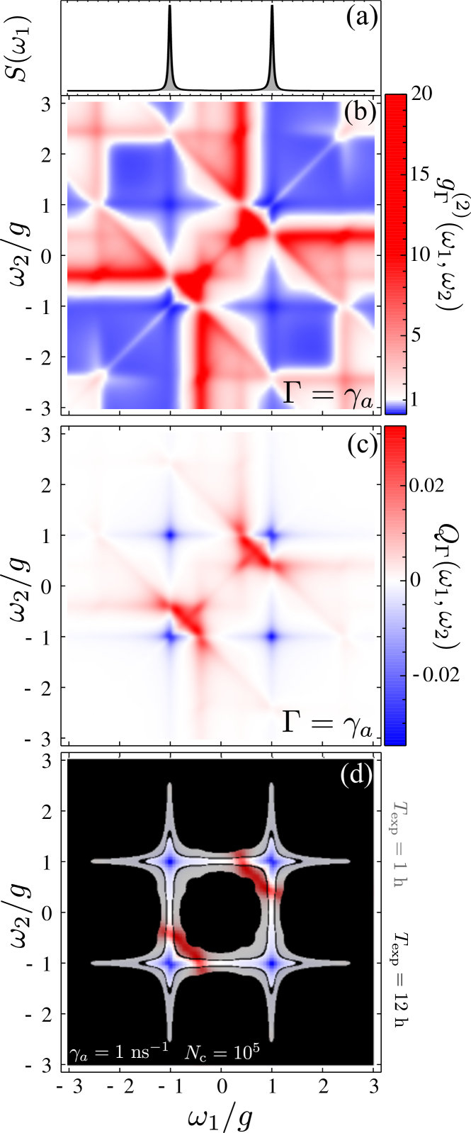
Figure 1: (Colour online) (a) One-photon spectrum for the JC system at low pumping, exhibiting the Rabi doublet of strong coupling. (b) The corresponding 2PS obtained by spanning $g_{\gamma_{a}}^{(2)}(\omega_{1},\omega_{2})$ over all frequencies (c) The corresponding frequency-resolved Mandel parameter $Q_{\gamma_{a}}(\omega_{1},\omega_{2})$, retaining only the well observable features. (d) $Q_{\gamma_{a}}(\omega_{1},\omega_{2})$ with a black (grey) mask superimposed to let appear only areas where $N_{c}\geq 10^{5}$ coincidence are obtained in a time $T_{\mathrm{exp}}=12$ h (1 h) for $\gamma_{a}=1/$ns. Parameters: $\gamma_{a}=0.1g$, $\gamma_{\sigma}=0.001g$ and $P_{\sigma}=0.01\gamma_{a}$.

Our main theme in this text is illustrated in Fig. 1, starting with the 2PS of the JC (b) under weak incoherent pumping in the regime of spontaneous emission del Valle et al. (2009); Poshakinskiy and Poddubny (2014), in which case its spectral lineshape is simply the Rabi doublet (a). The physical meaning of this correlation map is amply discussed in Ref. Gonzalez-Tudela et al. (2013). It is enough for our discussion to highlight the main phenomenology, namely the set of horizontal and vertical lines, that correspond to transitions between real states, and antidiagonal lines $\omega_{1}+\omega_{2}=E_{2,\pm}-E_{0}$ that correspond to two-photon “leapfrog” emission from the second manifold with levels at energies $E_{2,\pm}$ and the ground state at energy $E_{0}$. The transitions at the Rabi frequency $\pm R_{1}\approx\pm g$ are all antibunched (blue on the figure), since they are dominated by the decay of one polariton from the lower manifold and one excitation cannot be split into two polaritons, while the lines at $(\sqrt{2}\pm 1)g$ are mainly bunched (red on the figure), since they correspond to a cascade from the second manifold. The presence of such cascade correlations in a regime of low excitations, where the second manifold has a vanishing probability to be excited, illustrates the somewhat artificial character of the 2PS. The problem really pertains to photon-correlations in general rather than to the inclusion of frequency, since they similarly predicts $g^{(2)}(0)=0$ regardless of the pumping intensity, that is to say, the system exhibits antibunching of its overall emission however small is the probability for two excitations to be present simultaneously, and therefore for photon blockade to enforce the antibunching Birnbaum et al. (2005). The same holds for the harmonic oscillator at vanishing pumping which still generates bunched statistics $g^{(2)}(0)=2$ regardless of the probability to reach two excitations in the system. The paradox arises from the fact that in the limit where the probability of two-photon effects vanishes, so does the possibility to perform a measurement, since there is no signal. Instead, if one considers the Mandel correlations, Eq. (4), that are shown in Fig. 1(c), one sees how the result makes more physical sense: most of the nonlinear features have disappeared or are considerably weakened in the regions where there is a strong signal (the correlations tend to die more slowly than the signal), and the remaining features are concentrated on antibunching between the peaks, as well as a trace of the bunching cascades. The leapfrog correlations are extremely strong, which is a general result in all systems, while the antibunching background that dominates the 2PS profile has now disappeared. It is also worth noting how the autocorrelation of each peak (along the diagonal) has the butterfly shape due to indistinguishability bunching enforced by filtering Gonzalez-Tudela et al. (2013), while cross-correlation between the two peaks feature a structureless, and therefore neater, antibunching. This could be of interest for single-photon emitters Deutsch et al. (2012).

Although the Mandel correlation spectrum, Fig. 1(c), appears more physical than the underlying 2PS, Fig. 1(b), the latter still presents us with a more fundamental physical picture. Indeed, we have merely tamed down the features, not removed them, and it is useful to keep track of correlations even though they are out of reach of an actual experiment. In any case, the 2PS could still be measured ideally and should better be regarded as a theoretical limiting case. The 2PS indeed converges to a unique result in the limit of vanishing pumping, thereby defining an unambiguous correlation map, while its Mandel counterpart tends to zero and the relative importance of bunching versus antibunching areas in Fig. 1(c) depend on one’s choice of the pumping rate. Finally, it is worth mentioning that by the time of writing this text, the 2PS of resonance fluorescence has already been measured in its entirety Peiris et al. (2015) even for a large splitting of the satellite peaks with spectral windows of little emission. It seems therefore reasonable that with the ever-increasing technological progress, all fundamental quantum optical emitters, even those with much smaller emission rates, will be likewise characterized.

III Valleys of accessible correlations

While $Q_{\Gamma}(\omega_{1},\omega_{2})$ provides a physically sound picture of which regions of the 2PS are the most favorable for observation, it also suffers from its own shortcomings. The arbitrary scale of $Q$ makes it difficult to attach to it a quantitative figure of merit. In this Section, we further delineate the valleys of accessible correlations based on a down-to-earth estimate of the numbers of coincidences that can be extracted from the emission.

Assuming no correlations, the possibility of detecting at least one coincidence in a time window $\Delta t$ at frequencies $\omega_{i}$, within the frequency windows $\Gamma_{i}$, is given by:

$$p=(1-e^{-n_{1}})(1-e^{-n_{2}})\,,$$ (6)

where $n_{i}=S_{\Gamma_{i}}(\omega_{i})\gamma\Delta t$ represents the number of filtered photons from a source that emits at a rate $\gamma$. For simplicity we always consider symmetric filters in this Section, $\Gamma_{1}=\Gamma_{2}$. Using that definition and assuming no further inefficiencies in detection, we can estimate the experimental time required to obtain a given number of random coincidences, $N_{c}$, as follows:

$$T_{\mathrm{exp}}=N_{c}\Delta t/p\,.$$ (7)

With this, we plot the regions that would be resolved with increasing experimental time, $T_{\mathrm{exp}}$. For example, assuming $\gamma_{a}=1$ ns^-1 as a quantum dot figure of merit Hennessy et al. (2007), we show in Fig. 1(d) the frequency-resolved Mandel parameter with a mask over the regions for which the number of coincidences is $N_{c}<10^{5}$ for a detection time of $T_{\mathrm{exp}}=1$ (gray) and $12$ hours (black) for $\Delta t=1/\Gamma$. This shows how the regions with a sizable number of coincidences reduce to those involving at least one peak, as expected. Therefore, a first experimental confirmation of these results could be to keep one branch of the setup on one peak, and correlate its input with that of the other branch sweeping the entire spectrum. This should display transitions from antibunching, no correlation, strong bunching, no correlation again and a weaker antibunching in the autocorrelation, due to indistinguishability bunching. For this set of parameters, the experiment would need to run stably for a longer time in order to collect the same amount of signal to observe also the leapfrog processes without intersecting with the peaks. There is a non-trivial interplay of the system parameters that helps/hinders the observation of correlations which we will be explored in Section IV.

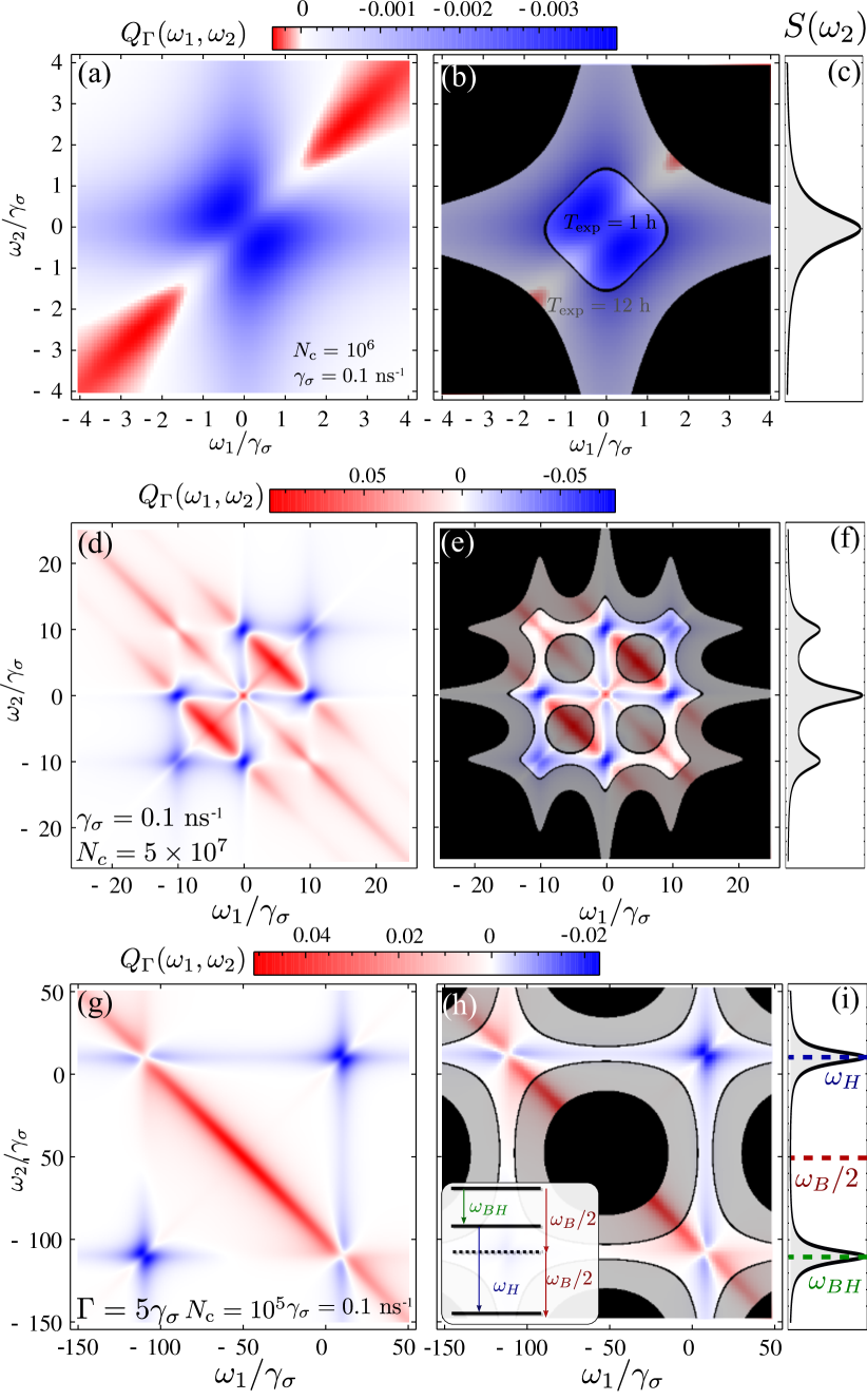
Figure 2: (Colour online) Panel (a-b) [(c)]: Mandel two-photon spectra [one-photon spectrum] for an incoherently pumped two-level system with $P_{\sigma}=0.01\gamma_{\sigma}$, $\gamma_{\sigma}=0.1$ ns^-1 and $\Gamma=\gamma_{\sigma}$. In Panel (b) we introduce a black (grey) mask for the points where $N_{c}<10^{6}$ in a time $T_{\mathrm{exp}}=12$ h (1 h). Panel (d-e) [(f)]: Mandel two-photon spectra [one-photon spectrum] for a coherently driven two-level system with $\Omega_{\sigma}=5\gamma_{\sigma}$, $\gamma_{\sigma}=0.1$ ns^-1 and $\Gamma=\gamma_{\sigma}$. In Panel (e) we introduce a black (grey) mask for the points where $N_{c}<5\times 10^{7}$ in a time $T_{\mathrm{exp}}=12$ h (1 h). Panel (g-h) [(i)]: Mandel two-photon spectra [one-photon spectrum] for an incoherently pumped biexciton system with $P_{\sigma}=\gamma_{\sigma}$, $\chi=100\gamma_{\sigma}$, $\gamma_{\sigma}=0.1$ ns^-1 and $\Gamma=5\gamma_{\sigma}$. In Panel (h) we introduce a black (grey) mask for the points where $N_{c}<5\times 10^{5}$ in a time $T_{\mathrm{exp}}=12$ h (1 h).

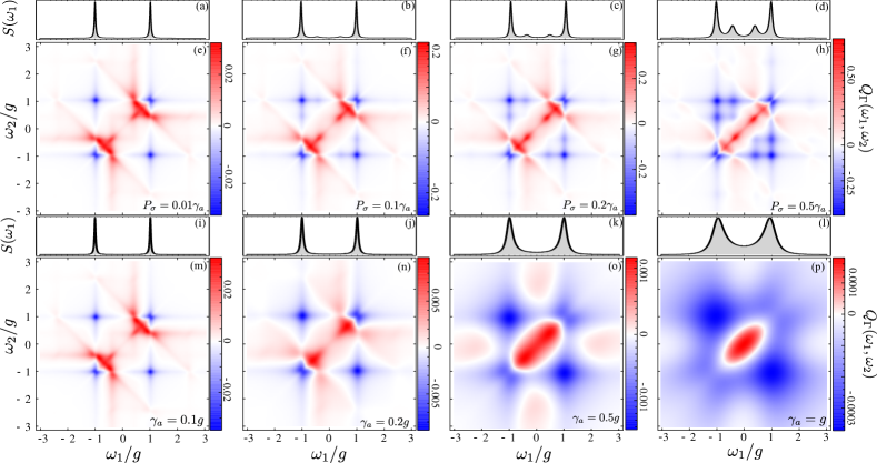
Figure 3: (Colour online) Panels (a-d): One-photon spectra for a JC system with $\gamma_{a}=0.1g$, $\gamma_{\sigma}=0.001g$ and increasing pumping $P_{\sigma}$ as depicted in the legend. Panels (e-f): Mandel two-photon spectra for a JC system with the same parameters as in (a-d). Panels (i-l): One-photon spectra for a JC system with $P_{\sigma}=0.01g$, $\gamma_{\sigma}=0.001g$ and increasing cavity decay rate, $\gamma_{a}$ as depicted in the legend. Panels (m-p): Mandel two-photon spectra for a JC system with the same parameters as in (i-l).

Before moving on to the optimization, we review other examples of nonlinear systems explored in Ref. Gonzalez-Tudela et al. (2013) in the light of the frequency resolved Mandel parameter and the estimated time to resolve it. We start by the most basic system that displays a non-trivial map of correlations, namely, the incoherently pumped two-level system which we recover by setting $g=0$ in the JC model. The one-photon spectrum of this system is a single Lorentzian peak with broadening $\Gamma_{\sigma}=\gamma_{\sigma}+P_{\sigma}$ as shown in Fig. 2(c). Its two-photon Mandel spectrum shows a butterfly shape of anticorrelation, typical of two-level systems Gonzalez-Tudela et al. (2013). By choosing $\Gamma=\gamma_{\sigma}$ and $\gamma_{\sigma}=0.1$ ns^-1, the analysis of the measuring time shows that a small region of frequency antibunching with $N_{c}>10^{6}$ would be observed within one hour, whereas most of the butterfly would be observed within $12$ hours for the same threshold of counts. While it is much more binding to observe, if filtering far in the tail of a two-level system, one should indeed observe bunching, against naive expectations.

Next, we consider a resonant coherent driving of the two-level system, described by Hamiltonian $H_{d}=\Omega_{\sigma}(\sigma+\sigma^{\dagger})$. In the weak driving regime, the system has been recently exploited to design ultra-narrow single-photon sources Nguyen et al. (2011); Matthiesen et al. (2012); He et al. (2013); makhonin14a; chip resonantly-driven quantum emitter with enhanced coherence (2014). In the strong-driving regime, which is the one that we focus on in this paper, the spectrum is the well known Mollow triplet Mollow (1969), as shown in Fig. 2(f). Frequency-resolved correlations for this system have been theoretically investigated in the past Wódkiewicz (1980); Arnoldus and Nienhuis (1983, 1984); Nienhuis (1993); Shatokhin and Kilin (2001) and even measured Aspect et al. (1980); Ulhaq et al. (2012); Weiler et al. (2013) before the concept of the 2PS was put forward. But in both the theoretical and experimental contexts, this was at the particular frequencies of the three peaks. Notwithstanding, interesting correlations arise mainly outside the peaks Gonzalez-Tudela et al. (2013); Sánchez-Muñoz et al. (2014), at the cost of a weaker signal. This has been confirmed experimentally Peiris et al. (2015) with the full reconstruction of the Mollow 2PS. Resonance fluorescence is indeed a system ideally suited to pioneer a comprehensive analysis of frequency photon correlations, since it is obtained in the strong-driving regime of an extremely quantum emitter, which implies a large emission of strongly correlated photons. Figure 2(e) shows that with $\gamma_{\sigma}=0.1$ ns^-1 and $\Gamma=\gamma_{\sigma}$, only within $1$ hour of experimental time, the regions with $N_{c}>5\times 10^{7}$ unveils all the horizontal and vertical grid of correlations and great part of the leapfrogs. It only takes $12$ hours to reveal the complete two-photon Mandel spectrum.

Finally, we consider a biexciton level scheme as described in Refs. del Valle et al. (2010, 2011); del Valle (2013) which is relevant in semiconductor quantum optics as it describes the typical level structure of quantum dots beyond the simplest two-level system picture Chen et al. (2002); Akimov et al. (2006); Ota et al. (2011). Focusing on a single polarization, it consist of a three-level scheme as depicted in the inset of Fig. 2(h), with a ground, an excitonic (at energy $\omega_{H}$) and a biexcitonic state whose energy ($\omega_{B}$) differs from the sum of its excitonic constituents by $\chi$ due to Coulomb interaction. The one-photon spectrum is then composed of two peaks (at energies $\omega_{H}$ and $\omega_{BH}=\omega_{B}-\omega_{H}$) which give rise to an interesting and rich landscape of two-photon correlations. The most prominent feature is the antidiagonal corresponding to the leapfrog between ground and biexciton state, $\omega_{1}+\omega_{2}=\omega_{B}=-\chi$ (assuming $\omega_{H}=0$ as the reference energy), with potential for applications in the generation of entangled photon pairs by frequency filtering del Valle (2013). With $\gamma_{\sigma}=0.1$ ns^-1 and setting the threshold at $N_{c}=10^{5}$ random coincidences, within one hour, the anticorrelation area and bunching of the one-photon transition peaks would be observable, whereas in $12$ hours most of its leapfrog structure would be revealed as well, especially by filtering on the sides of the one-photon peaks. Due to both its fundamental importance and practical applications, we will return to the problem of optimizing the observation of the leapfrog processes by changing both the intrinsic parameters as well as the filtering ones in Section V.

IV Optimization of correlations in the Jaynes-Cummings model

We now illustrate how to optimize photon correlations thanks to frequency filtering, in the particular case of the JC model. We do a qualitative analysis to avoid focusing the discussion on a particular set of experimental figures of merit. We consider the system parameters are variables for the optimization and postpone to next Section (and to other systems) the optimization through extrinsic parameters, e.g., the filters and detection time.

One parameter that can be easily modified is the incoherent pump rate, $P_{\sigma}$. The example of the previous Section was chosen to be well into the linear regime, i.e., with a very small pumping rate, namely $P_{\sigma}=0.01\gamma_{a}$. Increasing pumping has two interesting consequences for the observation of correlations:

1. signal increases,

2. the system enters the nonlinear regime.

In Fig. 3, upper row, the effect of increasing pumping is shown for both the spectral shape (a–d) and the Mandel parameter resolved in frequency (e–h). The spectra let appear inner peaks between the Rabi doublet, corresponding to transitions from the higher manifolds. The corresponding Mandel 2PS also develops new features at the same time as the overall intensity of the correlations increases, from $\sim 0.02$ with $P_{\sigma}=0.01\gamma_{a}$ to $\sim 0.5$ with $P_{\sigma}=0.5\gamma_{a}$ (note the change of the color scales). In particular, the higher manifolds become visible in antibunching only as they get populated, while they manifest themselves in bunching more clearly at low pumping. The Jaynes–Cummings fork provides a well-structured set of correlations between the peaks: the inner peaks emit bunched photons but are otherwise antibunched with each other, or with the remotest Rabi peak, and are uncorrelated with the other—closer—Rabi peak. When various manifolds are well populated, correlations are dominated by real-state transitions and virtual processes shy away in comparison.

Another parameter that is less easily tuned but that determines the strong-coupling property is the cavity decay rate. In the bottom row of Fig. 3, the effect of increasing $\gamma_{a}$ is shown, always keeping the system in the strong-coupling regime ($\gamma_{a}<4g$). This results in the structure smoothing out as well as the intensity of correlations dying (note, again, the color scales). The absolute scale of the Mandel correlations indeed decreases by one order of magnitude, but partly because the cavity gets less populated, and increasing pumping could compensate for that. For $\gamma_{a}=0.5g$ the leapfrog antidiagonal have disappeared and for $\gamma_{a}=g$, only the anticorrelation between the Rabi peaks have survived, surrounding a region of indistinguishability bunching. To track more quantitatively how the frequency-resolved correlations evolve with the cavity decay rate, we show in Fig. 4(a) the value of $Q_{\gamma_{a}}$ for pairs of frequencies corresponding to filtering the Rabi peaks. To show that there is some difference due to indistinguishability bunching in the case of autocorrelation, we present both the filtering for the same Rabi peak (in solid black) and for the two Rabi peaks (dashed red). For $\gamma_{a}\geq 4g$, when the system reaches the weak-coupling regime, frequency-filtered correlations collapse into a single curve since there are no longer polariton modes in the system. It is instructive in this case to plot $g^{(2)}_{\gamma_{a}}(R_{1},\pm R_{1})$ together with the standard $g^{(2)}$ (dotted blue) as shown in the inset of Fig. 4(a). The difference in this case between filtering the same peak or cross-correlating them becomes significant. As already observed, frequency filtering the Rabi peaks improves antibunching as compared to non-filtered correlations, as we are discarding the frequency regions with bunched photons. This is another instance of how frequency filtering can be used to harness correlations. Note also that worsening the cavity quality factor betters the overall antibunching while it spoils the peaks antibunching.

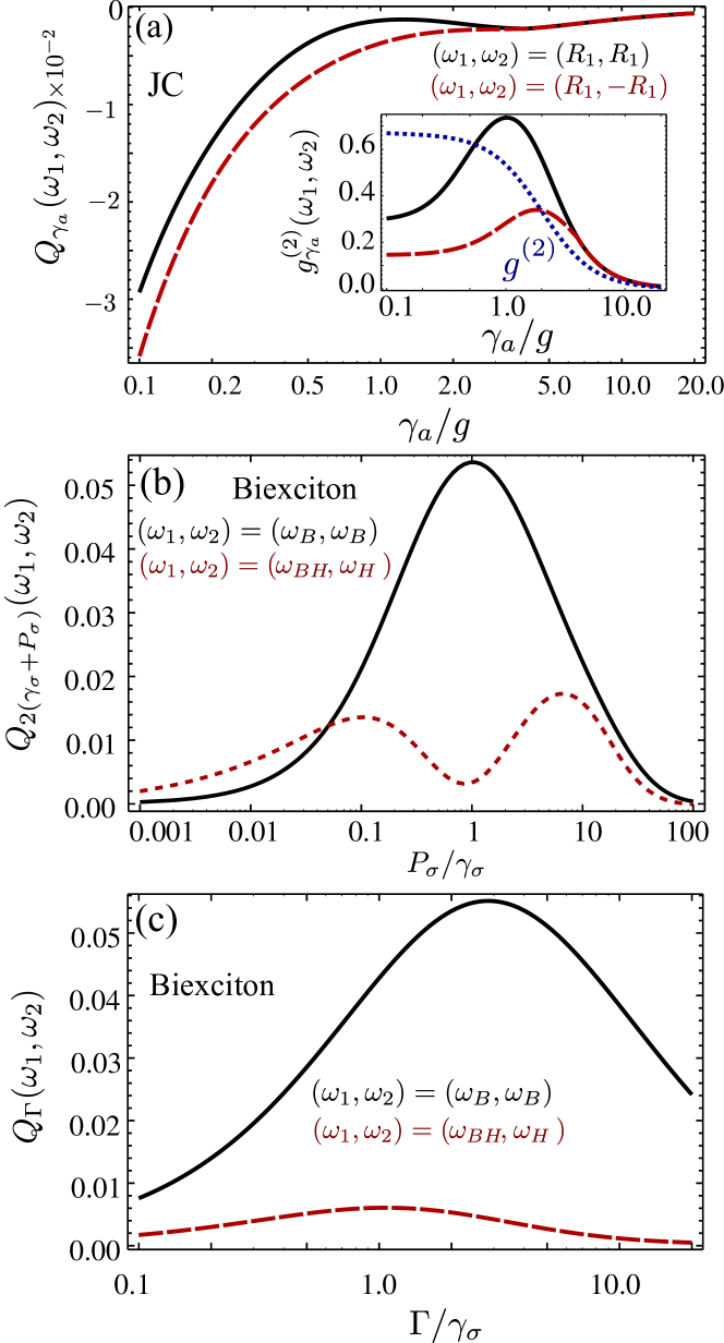
Figure 4: (Colour online) (a) $Q_{\gamma_{a}}(\omega_{1},\omega_{2})$ as a function of $\gamma_{a}$ for a JC system with $P_{\sigma}=0.01\gamma_{a}$, $\gamma_{\sigma}=0.001g$ for pair of frequencies $(R_{1},R_{1})$ (solid black), $(R_{1},-R_{1})$ (dashed red). Inset: $g_{\gamma_{a}}^{(2)}(\omega_{1},\omega_{2})$ for the same parameters, together with standard photon correlation $g^{(2)}(0)$ (dotted blue). (b) $Q_{\Gamma}(\omega_{1},\omega_{2})$ as a function of $P_{\sigma}$ for a biexciton cascade with the same parameters as in Fig. 2 and $\Gamma=2(\gamma_{\sigma}+P_{\sigma})$, for pair a of frequencies as indicated in inset. (c) $Q_{\Gamma}(\omega_{1},\omega_{2})$ as a function of $\Gamma$, with the same parameter of Fig. 2.

V Optimization of correlations in a biexciton cascade

We now study photon correlations in a biexciton cascade. To link with the previous discussion on the JC, we show in Fig. 4(b) the dependence on the pumping rate for two configurations, letting here the frequency window grow with the pumping as $\Gamma=2(\gamma_{\sigma}+P_{\sigma})$. The two configurations are filtering the leapfrog transition at the biexciton frequency (in solid black) and the biexciton-exciton cascade (in dashed red). Both transitions are bunched, $Q_{\Gamma}>0$, due to their two-photon cascade character. However, the one that corresponds to the leapfrog process exhibits a clear optimal pumping intensity, at $P_{\sigma}\sim 1.5\gamma_{\sigma}$, whereas the one-photon transitions exhibit two local maxima at around $P_{\sigma}\sim 0.2\gamma_{\sigma}$ and $P_{\sigma}\sim 8\gamma_{\sigma}$, that follow the successive growth of the exciton and biexciton populations. The low pumping regime leads to $Q_{\Gamma}\rightarrow 0$ due to the small emission whereas in the high pumping case this is because one recovers the standard photon correlations $g^{(2)}(0)\approx 1$.

V.1 Asymmetric filters

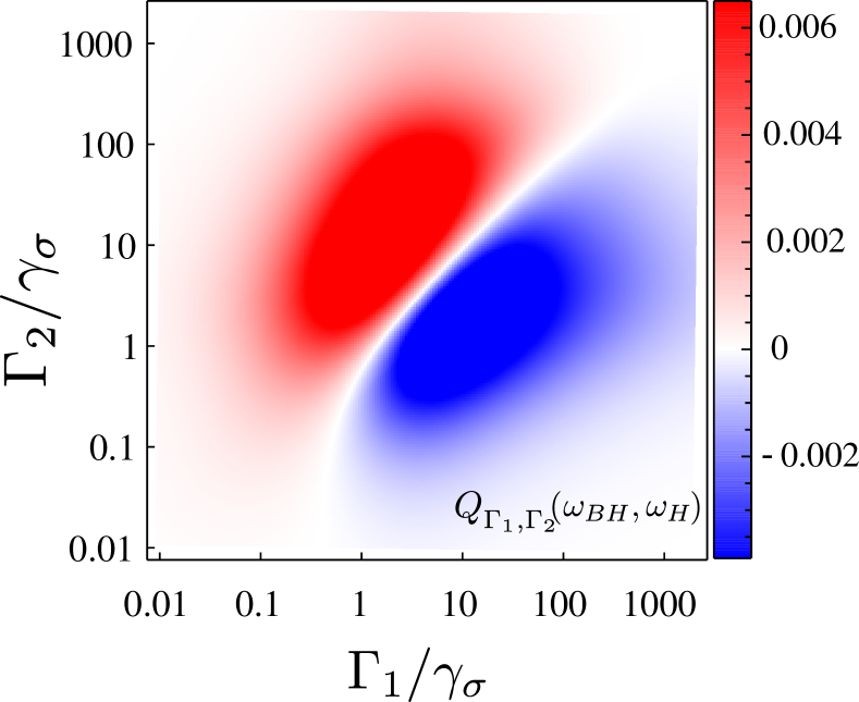
Figure 5: (Colour online) Mandel parameter $Q_{\Gamma_{1},\Gamma_{2}}(\omega_{BH},\omega_{H})$ when filtering the two peaks of the biexciton-exciton cascade as a function of the widths of the spectral windows. The diagonal corresponds to the typical case of identical filters. Stronger correlations and of a varying nature are however obtained for asymmetric filters. Parameters are the same as for Fig. 2.

We discuss in more details how the filter linewidth affects the correlations. In Fig. 4(c), we show the dependence with the filters linewidth $\Gamma$ for correlations of the leapfrog cascade (solid black) and the biexciton-exciton cascade (dashed red). The leapfrog correlations strongly depend on the filter linewidth, due to the virtual nature of their transitions, with an optimum value at around $4\gamma_{\sigma}$. The biexciton-exciton cascade also displays a maximum $\Gamma\sim\gamma_{\sigma}$, but its dependence is much weaker. In both cases, and in contrast with $g^{(2)}_{\Gamma}(\omega_{1},\omega_{2})$ where smaller linewidths optimize leapfrog correlations, the compromise for signal requires larger filter linewidths to optimize the intensity of correlations.

In the analysis so far, we have always considered symmetric filters for the two frequencies: $\Gamma_{1}=\Gamma_{2}=\Gamma$. However, for a cascaded emission such as biexciton $\rightarrow$ exciton $\rightarrow$ ground state, it is worth exploring the situation where the filters are asymmetric, $\Gamma_{1}\neq\Gamma_{2}$. This is shown in Fig. 5, filtering the biexciton/exciton peaks for a situation where they have the same broadening and intensity ($P_{\sigma}=\gamma_{\sigma}$). Two areas of bunching/antibunching oppose each other depending on the relative value of $\Gamma_{1}$ vs $\Gamma_{2}$, separated by a frontier of no-correlation that roughly correspond to the case of symmetric filters, showing the interest in lifting this limitation even when both spectral peaks are equal. Such a structure is typical of photon cascades. From the level structure, the natural order of the cascade makes it indeed likely to detect a photon first of frequency $\omega_{BH}$ then of $\omega_{H}$. Since an $\omega_{BH}$ [$\omega_{H}$] photon, filtered with $\Gamma_{1}$ [$\Gamma_{2}$], is the first [second] photon in the cascade, if $\Gamma_{2}>\Gamma_{1}$ the time spent by the photon in filter $\omega_{1}$ is larger than the one $\omega_{2}$ which is favouring the simultaneous detection of the two photons of the cascade, and therefore, yields a strong bunching. In the opposite regime, when $\Gamma_{1}>\Gamma_{2}$, the $\omega_{BH}$ photon spends less time in the filter preventing the simultaneous detection of the two photons of the cascade and therefore yielding strong antibunching in the Mandel parameter. There is an optimum value to observe either antibunching/bunching—as a rule of thumb, an order of magnitude difference—since ultimately the observations of correlations quenches for very broad/asymmetric filters. This loss of correlations is due, interestingly, to the overlap of the filtering windows.

V.2 Delayed correlations

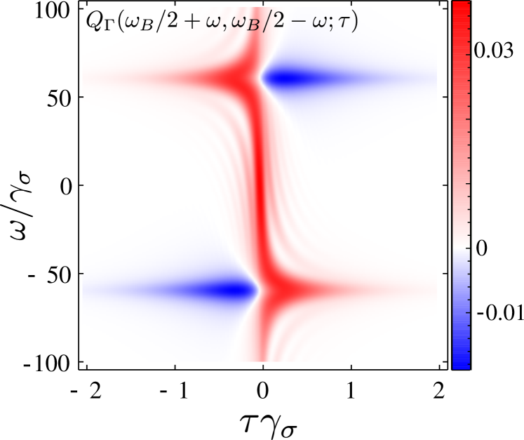
Figure 6: (Colour online) Mandel parameter $Q_{\Gamma}(\omega_{B}/2+\omega,\omega_{B}/2-\omega;\tau)$ when filtering the leapfrog processes (antidiagonal) of the biexciton-exciton cascade and as a function of autocorrelation time. This shows the contrast between leapfrog (virtual) processes where the correlations are symmetric in $\tau$ and with a fast decay, and real processes that, when intercepted by the filters, lead to characteristic antibunching-bunching transitions with a slow decay. Parameters are the same as in Fig. 2 except for $\Gamma=10\gamma_{\sigma}$.

We have also restricted our attention to $\tau=0$, i.e., coincidences. However, particularly for cascaded emission, it is to be expected that correlations are maximum at nonzero delay del Valle et al. (2012). To condense the bulk of the information into a single figure (Fig. 6), we consider the joint frequency- and time-resolved Mandel 2PS along the leapfrog antidiagonal of Fig. 2 (e-f), $Q_{\Gamma}(\omega_{B}/2+\omega,\omega_{B}/2-\omega;\tau))$ for $\Gamma=10\gamma_{\sigma}$. In this line lies the information of both the leapfrogs and the one-photon cascade. Leapfrog emission is maximum at $\omega=0$ del Valle (2013) and is symmetric in $\tau$, which is typical of second-order processes where the photons, being virtual, have no time order. Due to this symmetry, the optimal delay to observe correlations in this case is $\tau=0$, and they decay with the filter timescale $1/\Gamma$. Contrarily, the biexciton-exciton photon cascade, appearing at $\omega=\{\omega_{BH},\omega_{H}\}$, is strongly asymmetric, as clearly shown in Fig. 6. It shows a bunching/antibunching behaviour as expected for cascades of real transitions, where there is a definite temporal order in the emission. In this case, the optimal value to observe strong bunching/antibunching is $\tau\sim 1/\Gamma$ and the correlations ultimately decay in the intrinsic timescale of the system given by $1/\gamma_{\sigma}$. The different timescales where correlations survive between leapfrog and normal cascaded emissions is another consequence of their different physical origin.

V.3 Combining the parameters

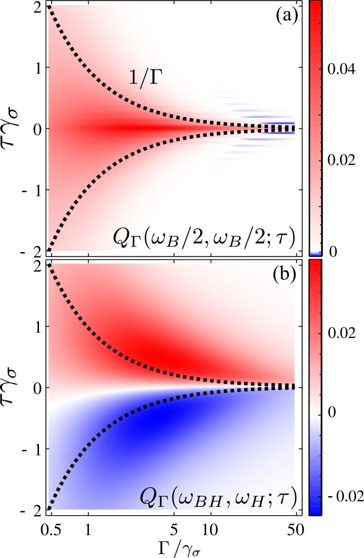
Figure 7: (Colour online) (a) Mandel parameter $Q_{\Gamma}(\omega_{B}/2,\omega_{B}/2;\tau)$ when filtering the leapfrog processes of the biexciton-exciton cascade and (b) $Q_{\Gamma}(\omega_{BH},\omega_{H};\tau)$ when filtering the two peaks, as a function of correlation time $\tau$ and filters linewidth $\Gamma$. This highlights again the difference between real and virtual processes. An optimum value of the filters linewidth can be found for the case of real state transitions. Parameters are the same as for Fig. 2.

Finally, after having explored separately both the dependence on the filter linewidth, $\Gamma$, and the temporal delay of the photons, $\tau$, one can naturally think of combining them to optimize correlations cumulatively. In Fig. 7, we show the joint $\tau$ and $\Gamma$ dependence of the frequency-resolved Mandel parameter for the two more relevant cases: the leapfrog two-photon cascade in (a) and the consecutive one-photon transitions in (b). As previously discussed, the temporal shape of the leapfrog cascade is a symmetric decay of correlations within timescale $1/\Gamma$, as shown in the figure. As $\Gamma$ increases, so does the decay rate of the correlations (the correlation time and the filters linewidth are roughly in inverse proportion, as shown by the dotted lines which are $1/(\Gamma/\gamma_{\sigma})$). The $\tau=0$ correlation also strongly decreases and is eventually surrounded by antibunching oscillations in $\tau$, that correspond to the fast off-resonance one-photon transitions. For the set of parameters chosen here, the optimal correlations are to be found at $\tau=0$ and for $\Gamma\sim 3\gamma_{\sigma}$. Also as discussed previously, in the consecutive one-photon cascade in Fig. 7(b), the temporal shape exhibits a typical asymmetric bunching/antibunching shape. The pattern is fairly robust but can indeed be magnified by the appropriate choice of filters (we consider here symmetric filters for simplicity). The temporal decay occurs this time approximately within a time scale of $1/\gamma_{\sigma}$, while the maximum value for the correlations, both bunching and antibunching, is obtained at $\tau\sim 1/\Gamma$. In this case, the maximum is found at $\Gamma\sim 3\gamma_{\sigma}$ and $\tau\sim 1/\Gamma$. Note that correlations are optimised for filters with a width equal to the spectral peaks ($3\gamma_{\sigma}$ for our choice of parameters).

VI Summary and Conclusions

Summing up, filtering the photons emitted by a quantum source has a dramatic impact on their correlations. Strong correlations are often found in regions of the spectrum where there is a weak emission, making their experimental detection particularly difficult, since this implies coincidences of rare events. We have introduced a “frequency-resolved Mandel parameter” as well as a quantitative estimate of the time required to accumulate a given number of coincidences, to address this problematic for several paradigmatic non-linear quantum systems. We have shown the considerable flexibility opened by frequency-filtering, either in energy or in time, with possibilities to enhance correlations by varying filters linewidths (possibly asymmetrically), temporal windows of detections and system parameters (such as pumping). Depending on whether the correlations originate from real states transitions or involve virtual processes, different strategies should be adapted, corresponding to their intrinsically different character. With the recent experimental demonstration of the underlying physics Peiris et al. (2015), the field of two-photon spectroscopy is now ripe to power applications and optimize resources based on photon correlations.