Optimal quasi-Monte Carlo rules on order $2$ digital nets for the numerical integration of multivariate periodic functions

Abstract

We investigate quasi-Monte Carlo rules for the numerical integration of multivariate periodic functions from Besov spaces $S^{r}_{p,q}B(\mathbb{T}^{d})$ with dominating mixed smoothness $1/p<r<2$. We show that order 2 digital nets achieve the optimal rate of convergence $N^{-r}(\log N)^{(d-1)(1-1/q)}$. The logarithmic term does not depend on $r$ and hence improves the known bound of Dick [6] for the special case of Sobolev spaces $H^{r}_{\text{mix}}(\mathbb{T}^{d})$. Secondly, the rate of convergence is independent of the integrability $p$ of the Besov space, which allows for sacrificing integrability in order to gain Besov regularity. Our method combines characterizations of periodic Besov spaces with dominating mixed smoothness via Faber bases with sharp estimates of Haar coefficients for the discrepancy function of order $2$ digital nets. Moreover, we provide numerical computations which indicate that this bound also holds for the case $r=2$.

1 Introduction

Quasi-Monte Carlo methods play an important role for the efficient numerical integration of multivariate functions. Many real world problems, for instance, from finance, quantum physics, meteorology, etc., require the computation of integrals of $d$-variate functions where $d$ may be very large. This can almost never be done analytically since often the available information of the signal or function $f$ is highly incomplete or simply no closed-form solution exists. A quasi-Monte Carlo rule approximates the integral $I(f)=\int_{[0,1]^{d}}f(x)\,\mathrm{d}x$ by (deterministically) averaging over $N$ function values taken at fixed points $X_{N}=\{x^{1},\ldots,x^{N}\}$, i.e.,

$$I_{N}(X_{N},f):=\frac{1}{N}\sum\limits_{i=1}^{N}f(x^{i}),$$

where the $d$-variate function $f$ is assumed to belong to some (quasi-)normed function space $F_{d}\subset C([0,1]^{d})$. Since the integration weights $\frac{1}{N}$ are positive and sum up to $1$, QMC integration is stable and easy to implement which significantly contributed to its popularity. The QMC-optimal worst-case error with respect to the class $F_{d}$ is given by

$$\mbox{QMC}_{N}(F_{d}):=\inf\limits_{\begin{subarray}{c}X_{N}\subset[0,1]^{d}\\ \#X_{N}=N\end{subarray}}\sup\limits_{\|f|F_{d}\|\leq 1}|I(f)-I_{N}(X_{N},f)|\,.$$ (1.1)

In this paper we investigate the asymptotical properties of Dick’s construction [6] of order $\sigma$ digital nets $X_{N}$ where $N=2^{n}$. This construction has recently attracted much attention in the area of uncertainty quantification [11, 10]. In the present paper we are interested in the asymptotic optimality of those higher order nets in the sense of (1.1) with respect to $F_{d}$ being a periodic Nikol’skij-Besov space $S^{r}_{p,q}B(\mathbb{T}^{d})$ with smoothness $r$ larger than $1$ and less than $2$.

Dick [6] showed for periodic Sobolev spaces $H^{r}_{\text{mix}}(\mathbb{T}^{d})=S^{r}_{2,2}B(\mathbb{T}^{d})$

$$\mbox{QMC}_{N}(H^{r}_{\text{mix}}(\mathbb{T}^{d}))\lesssim N^{-\lfloor r\rfloor}(\log N)^{d\lfloor r\rfloor-1}\quad,\quad N\geq 2\,,$$ (1.2)

if $1/2<r\leq\sigma$. He also considered non-periodic integrands, see [7]. However, well-known asymptotically optimal results for the integration of periodic Sobolev functions, see for instance the survey [50], show that the exponent of the $\log$ should be independent of the smoothness parameter $r$, namely $(d-1)/2$. In that sense, (1.2) is far from being optimal. Nevertheless, Dick’s bound (1.2) beats the well-known sparse grid bound if $r$ is an integer and $d$ is large. The latter bound involves the log-term $(\log N)^{(d-1)(r+1/2)}$, see [20, 51] and (1.8) below, which represents the best possible rate among all cubature formulas taking function values on a sparse grid [20].

The aim of this paper is twofold. On the one hand we aim at showing the sharp relation

$$\mbox{QMC}_{N}(H^{r}_{\text{mix}}(\mathbb{T}^{d}))\asymp N^{-r}(\log N)^{(d-1)/2}\quad,\quad N\geq 2\,,$$ (1.3)

if $1/2<r<2$ by proving the asymptotical optimality of order $2$ digital nets for (1.1). On the other hand we would like to extend (1.3) to periodic Nikol’skij-Besov spaces with dominating mixed smoothness $S^{r}_{p,q}B(\mathbb{T}^{d})$, namely,

$$\mbox{QMC}_{N}(S^{r}_{p,q}B(\mathbb{T}^{d}))\asymp N^{-r}(\log N)^{(d-1)(1-1/q)}\quad,\quad N\geq 2\,,$$ (1.4)

for $1/p<r<2$, see Definition 2.3 below. An immediate feature of these error bounds is the fact that the $\log$-term disappears in case $q=1$. Besov regularity is the correct framework when it comes to integrands of the form

$$f(x)=\max\{0,g(x)\}\quad,\quad x\in{\mathbb{R}}^{d}\,,$$ (1.5)

so-called kink functions, which often occur in mathematical finance, e.g. the pricing of a European call option, whose pay-off function possesses a kink at the strike price, see e.g. [22, Chapter 1]. In general, one can not expect Sobolev regularity higher than $r=3/2$. However, when considering Besov regularity we can achieve smoothness $r=2$. Indeed, the simple example $f(t)=\max\{0,t-1/2\}$ belongs to $B^{2}_{1,\infty}([0,1])$ while its Sobolev regularity $H^{s}$ is below $s=3/2$. In a sense, one sacrifices integrability for gaining regularity. Looking at the bound (1.4) above, we see that cubature methods based on order $2$ digital nets benefit from higher Besov regularity while the integrability $p$ does not enter the picture.

Apart from that, spaces of this type have a long history in the former Soviet Union, see [1, 39, 43, 49] and the references therein. The scale of spaces $S^{r}_{p,q}B(\mathbb{T}^{d})$ contains several important special cases of spaces with mixed smoothness like Hölder-Zygmund spaces $(p=q=\infty)$, the above mentioned Sobolev spaces $(p=q=2)$ and the classical Nikol’skij spaces $(q=\infty)$. Note that Sobolev spaces $S^{r}_{p}H(\mathbb{T}^{d})$ with integrability $1<p<\infty$ and $r>0$ are not contained in the Besov scale. They represent special cases of Triebel-Lizorkin spaces $S^{r}_{p,q}F(\mathbb{T}^{d})$ if $q=2$. However, classical embedding theorems allow to reduce the question for $\mbox{QMC}_{N}(S^{r}_{p}H(\mathbb{T}^{d}))$ to (1.4) in the case of “large” smoothness $r>\max\{1/p,1/2\}$, see Corollary 5.6 below. For a complete study of asymptotical error bounds (including the case of “small” smoothness) of numerical integration in spaces $S^{r}_{p}H(\mathbb{T}^{d})$ and $S^{r}_{p,q}F(\mathbb{T}^{d})$ we refer to the recent preprint [53]. See also Remark 5.7 below.

The by now classical research topic of numerically integrating periodic functions goes back to the work of Korobov [28], Hlawka [27], and Bakhvalov [3] in the 1960s and was continued later by Temlyakov, see [46, 47, 48], Dubinin [17, 18] and Skriganov [44]. See also the survey articles Temlyakov [50] and Novak [40]. In particular, Temlyakov [46, 47] used the classical Korobov lattice rules in order to obtain for $1/2<r\leq 1$

$$N^{-r}(\log N)^{(d-1)}\lesssim\mbox{QMC}_{N}(S^{r}_{2,\infty}B(\mathbb{T}^{d}))\lesssim N^{-r}(\log N)^{(d-1)(r+1/2)}$$ (1.6)

as well as

$$N^{-r}(\log N)^{(d-1)/2}\lesssim\mbox{QMC}_{N}(H^{r}_{\text{mix}}(\mathbb{T}^{d}))\lesssim N^{-r}(\log N)^{(d-1)r}$$ (1.7)

for $N\geq 2$. In contrast to the quadrature of univariate functions, where equidistant point grids lead to optimal formulas, the multivariate problem is much more involved. In fact, the choice of proper sets $X_{N}\subset\mathbb{T}^{d}$ of integration nodes in the $d$-dimensional unit cube is the essence of “discrepancy theory” [14, 13] and connected with deep problems in number theory, already for $d=2$.

Recently, Triebel [51, 52] and, independently, Dũng [19] brought up the framework of tensor Faber bases for functions of the above type. The main feature is the fact that the basis coefficients are linear combinations of function values. The corresponding series expansion is thus extremely useful for sampling and integration issues. Triebel was actually the first who investigated cubature formulas for spaces $S^{r}_{p,q}B(Q_{d})$ of functions on the unit cube $Q_{d}:=[0,1]^{d}$. By using more general cubature formulas of type (1.9) below (with non-equal weights) and nodes from a sparse grid Triebel obtained the two-sided estimate

$$N^{-r}(\log N)^{(d-1)(1-1/q)}\lesssim\mbox{Int}_{N}(S^{r}_{p,q}B(Q_{d}))\lesssim N^{-r}(\log N)^{(d-1)(r+1-1/q)}$$ (1.8)

if $1\leq p,q\leq\infty$ and $1/p<r<1+1/p$. Here, $\mbox{Int}_{N}$ denotes the optimal worst-case integration error where one admits general (not only QMC) cubature formulas of type

$$\Lambda_{N}(X_{N},f):=\sum\limits_{i=1}^{N}\lambda_{i}f(x^{i})\,.$$ (1.9)

In contrast to $S^{r}_{p,q}B(\mathbb{T}^{d})$, the space $S^{r}_{p,q}B(Q_{d})$ consists of non-periodic functions on $Q_{d}:=[0,1]^{d}$. The questions remain how to close the gaps in the power of the logarithms in (1.6), (1.7), and (1.8) and what (if existing) are optimal QMC algorithms?

This question has partly been answered by the first and second named authors for a subclass of $S^{r}_{p,q}B(Q_{d})$ with $1/p<r\leq 1$, namely those functions $S^{r}_{p,q}B(Q_{d})^{\urcorner}$ with vanishing boundary values on the “upper and right” boundary faces, by showing that the lower bound in (1.8) is sharp for quasi-Monte Carlo methods based on Chen-Skriganov points, see [24, 31, 32, 30]. Furthermore, together with M. Ullrich the last named author recently observed, that the classical Frolov method is optimal in all (reasonable) spaces $S^{r}_{p,q}B(Q_{d})^{\square}$ and $S^{r}_{p,q}F(Q_{d})^{\square}$ of functions with homogeneous boundary condition, see [53]. Note, that Frolov’s method is an equal-weight cubature formula of type (1.9) with nodes from a lattice (not a lattice rule). In a strict sense, Frolov’s method is not a QMC method since the weights $\lambda_{i}$ do not sum up to $1$.

In this paper we investigate special QMC methods for periodic Nikol’skij-Besov spaces on $\mathbb{T}^{d}$ and answer the above question partly. The picture is clear in case $d=2$, i.e., for spaces on the $2$-torus $\mathbb{T}^{2}$. In fact, we know that the lower bound in (1.8) is even sharp for all $r>1/p$, see [48, 56, 20]. The optimal QMC rule in case $1/p<r<2$ is based on Hammersley points [56], which provide the optimal discrepancy in this setting [24]. This paper can be seen as continuation of [56] for the higher-dimensional situation by adopting methods from [24, 32, 31, 33].

We will prove the optimality of QMC methods based on order $2$ digital nets in the framework of periodic Besov spaces with dominating mixed smoothness if $1/p<r<2$. Due to the piecewise linear building blocks, we can not expect to get beyond $1/p<r<2$ with our proof method even when taking higher order digital nets. Therefore, this restriction seems to be technical and may be overcome by using smoother basis atoms like piecewise polynomial B-splines [19].

We illustrate our theoretical results with numerical computations in the Hilbert space case $H^{r}_{{\rm mix}}(\mathbb{T}^{d})$ in several dimensions $d$ and for different smoothness parameters $r$. In the case of integer smoothness we exploit an exact representation formula for the worst-case integration error of an arbitrary cubature rule. A numerical evaluation of this formula indicates that the results in Theorem 5.3 below keep valid for $r=2$. The comparison with other widely used cubature rules such as sparse grids and Halton points in all dimensions and Fibonacci lattices in dimension $d=2$ shows that order 2 digital nets perform very well not only asymptotically but already for a relatively small number of sample points. Finally, we consider a simple test function which is a tensor product of univariate functions of the form (1.5). Expressing the regularity of such functions in Besov spaces of mixed smoothness allows the correct prediction of the asymptotical rate of the numerical integration error which is verified by our numerical experiments. However, the applicability of order $2$ nets to real-world problems from option pricing etc., where the kinks are not necessarily axis aligned, requires further research.

The paper is organized as follows. In Section 2 we introduce the function spaces of interest and provide the necessary characterizations and properties. The classical definition by mixed iterated differences will turn out to be of crucial importance. In Section 3 we deal with the Faber and Haar basis, especially with their hyperbolic (anisotropic) tensor product. The main tools represent Propositions 3.4 and 3.5 where the function space norm is related to the Faber coefficient sequence space norm and vice versa. In Section $4$ we recall Dick’s construction of higher order digital nets and compute the Haar coefficients of the associated discrepancy function. We continue in Section $5$ by interpreting the Haar coefficients of the discrepancy function in terms of integration errors for tensorized Faber hat functions. Combining those estimates with the Faber basis expansion and the characterization from Section $3$ we obtain our main results in Theorem 5.3. Finally, Section $6$ provides the numerical results.

Notation. As usual $\mathbb{N}$ denotes the natural numbers, $\mathbb{N}_{0}=\mathbb{N}\cup\{0\}$, $\mathbb{N}_{-1}=\mathbb{N}_{0}\cup\{-1\}$, $\mathbb{Z}$ denotes the integers, $\mathbb{R}$ the real numbers, and $\mathbb{C}$ the complex numbers. The letter $d$ is always reserved for the underlying dimension in $\mathbb{R}^{d},\mathbb{Z}^{d}$ etc. We denote by $\langle x,y\rangle$ the usual Euclidean inner product and inner products in general. For $a\in\mathbb{R}$ we denote $a_{+}:=\max\{a,0\}$. For $0<p\leq\infty$ and $x\in{\mathbb{R}}^{d}$ we denote $|x|_{p}=(\sum_{i=1}^{d}|x_{i}|^{p})^{1/p}$ with the usual modification in the case $p=\infty$. We further denote $x_{+}:=((x_{1})_{+},\ldots,(x_{d})_{+})$ and $|x|_{+}:=|x_{+}|_{1}$. By $(x_{1},\ldots,x_{d})>0$ we mean that each coordinate is positive. By $\mathbb{T}$ we denote the torus represented by the interval $[0,1]$, where the end points are identified. If $X$ and $Y$ are two (quasi-)normed spaces, the (quasi-)norm of an element $x$ in $X$ will be denoted by $\|x|X\|$. The symbol $X\hookrightarrow Y$ indicates that the identity operator is continuous. For two sequences $a_{n}$ and $b_{n}$ we will write $a_{n}\lesssim b_{n}$ if there exists a constant $c>0$ such that $a_{n}\leq c\,b_{n}$ for all $n$. We will write $a_{n}\asymp b_{n}$ if $a_{n}\lesssim b_{n}$ and $b_{n}\lesssim a_{n}$.

2 Periodic Besov spaces with dominating mixed smoothness

Let $\mathbb{T}^{d}$ denote the $d$-torus, represented in the Euclidean space $\mathbb{R}^{d}$ by the cube $\mathbb{T}^{d}=[0,1]^{d}$, where opposite points are identified. That means $x,y\in\mathbb{R}^{d}$ are identified if and only if $x-y=k$, where $k=(k_{1},\ldots,k_{d})\in\mathbb{Z}^{d}$. The computation of the Fourier coefficients of an integrable $d$-variate periodic function is performed by the formula

$$\hat{f}(k)=\int_{\mathbb{T}^{d}}f(x)e^{-i2\pi k\cdot x}\,{\rm d}x\quad,\quad k\in\mathbb{Z}^{d}\,.$$

Let further denote $L_{p}(\mathbb{T}^{d})$, $0<p\leq\infty$, the space of all measurable functions $f:\mathbb{T}^{d}\rightarrow\mathbb{C}$ satisfying

$$\|f\|_{p}=\Big{(}\,\int_{\mathbb{T}^{d}}|f(x)|^{p}\,{\rm d}x\Big{)}^{1/p}<\infty$$

with the usual modification in case $p=\infty$. The space $C(\mathbb{T}^{d})$ is often used as a replacement for $L_{\infty}(\mathbb{T}^{d})$. It denotes the collection of all continuous and bounded periodic functions equipped with the $L_{\infty}$-topology.

2.1 Definition and basic properties

In this section we give the definition of Besov spaces with dominating mixed smoothness on $\mathbb{T}^{d}$ based on a dyadic decomposition on the Fourier side. We closely follow [43, Chapter 2]. To begin with, we recall the concept of a dyadic decomposition of unity. The space $C^{\infty}_{0}(\mathbb{R}^{d})$ consists of all infinitely many times differentiable compactly supported functions.

Definition 2.1.

Let $\Phi(\mathbb{R})$ be the collection of all systems $\varphi=\{\varphi_{n}(x)\}_{n=0}^{\infty}\subset C^{\infty}_{0}(\mathbb{R}^{d})$ satisfying

(i) ${{\rm supp\,}}\,\varphi_{0}\subset\{x:|x|\leq 2\}$  ,

(ii) ${{\rm supp\,}}\,\varphi_{n}\subset\{x:2^{n-1}\leq|x|\leq 2^{n+1}\}\quad,\quad n=1,2,\ldots,$

(iii) For all $\ell\in\mathbb{N}_{0}$ it holds $\sup\limits_{x,n}2^{n\ell}\,|D^{\ell}\varphi_{n}(x)|\leq c_{\ell}<\infty$  ,

(iv) $\sum\limits_{n=0}^{\infty}\varphi_{n}(x)=1$ for all $x\in\mathbb{R}$.

Remark 2.2.

The class $\Phi(\mathbb{R})$ is not empty. We consider the following standard example. Let $\varphi_{0}(x)\in S(\mathbb{R})$ be a smooth function with $\varphi_{0}(x)=1$ on $[-1,1]$ and $\varphi_{0}(x)=0$ if $|x|>2$. For $n>0$ we define

$$\varphi_{n}(x)=\varphi_{0}(2^{-n}x)-\varphi_{0}(2^{-n+1}x).$$

It is easy to verify that the system $\varphi=\{\varphi_{n}(x)\}_{n=0}^{\infty}$ satisfies (i) - (iv).

Now we fix a system $\varphi=\{\varphi_{n}\}_{n\in\mathbb{Z}}\in\Phi(\mathbb{R})$, where we put $\varphi_{n}\equiv 0$ if $n<0$. For $j=(j_{1},\ldots,j_{d})\in\mathbb{Z}^{d}$ let the building blocks $f_{j}$ be given by

$$f_{j}(x)=\sum\limits_{k\in\mathbb{Z}^{d}}\varphi_{j_{1}}(k_{1})\cdots\varphi_{j_{d}}(k_{d})\hat{f}(k)e^{i2\pi k\cdot x}\quad,\quad x\in\mathbb{T}^{d}\,,j\in\mathbb{Z}^{d}\,.$$ (2.1)

Definition 2.3.

(Mixed periodic Besov and Sobolev space)
(i) Let $0<p,q\leq\infty$ and $r>\sigma_{p}:=(1/p-1)_{+}$. Then $S^{r}_{p,q}B(\mathbb{T}^{d})$ is defined as the collection of all $f\in L_{1}(\mathbb{T}^{d})$ such that

$$\|f|S^{r}_{p,q}B(\mathbb{T}^{d})\|^{\varphi}:=\Big{(}\sum\limits_{j\in\mathbb{N}_{0}^{d}}2^{|j|_{1}rq}\|f_{j}\|_{p}^{q}\Big{)}^{1/q}$$ (2.2)

is finite (usual modification in case $q=\infty$).
(ii) Let $1<p<\infty$ and $r>0$. Then $S^{r}_{p}H(\mathbb{T}^{d})$ is defined as the collection of all $f\in L_{p}(\mathbb{T}^{d})$ such that

$$\|f|S^{r}_{p}H(\mathbb{T}^{d})\|^{\varphi}:=\Big{\|}\Big{(}\sum\limits_{j\in\mathbb{N}_{0}^{d}}2^{|j_{1}|r2}|f_{j}(x)|^{2}\Big{)}^{1/2}\Big{\|}_{p}$$

is finite.

Recall, that this definition is independent of the chosen system $\varphi$ in the sense of equivalent (quasi-)norms. Moreover, in case $\min\{p,q\}\geq 1$ the defined spaces are Banach spaces, whereas they are quasi-Banach spaces in case $\min\{p,q\}<1$. For details confer [43, 2.2.4]. In this paper we are mainly concerned with spaces providing sufficiently large smoothness $(r>1/p)$ such that the elements (equivalence classes) in $S^{r}_{p,q}B(\mathbb{T}^{d})$ contain a continuous representative. We have the following elementary embeddings, see [43, 2.2.3].

Lemma 2.4.

Let $0<p<\infty$, $r\in\mathbb{R}$, and $0<q\leq\infty$.

(i) If $\varepsilon>0$ and $0<v\leq\infty$ then

$$S^{r+\varepsilon}_{p,q}B(\mathbb{T}^{d})\hookrightarrow S^{r}_{p,v}B(\mathbb{T}^{d})\,.$$

(ii) If $p<u\leq\infty$ and $r-1/p=t-1/u$ then

$$S^{r}_{p,q}B(\mathbb{T}^{d})\hookrightarrow S^{t}_{u,q}B(\mathbb{T}^{d})\,.$$

(iii) If $r>1/p$ then

$$S^{r}_{p,q}B(\mathbb{T}^{d})\hookrightarrow C(\mathbb{T}^{d})\,.$$

(iv) If $1<p<\infty$ and $r>0$ then

$$S^{r}_{p,\min\{p,2\}}B(\mathbb{T}^{d})\hookrightarrow S^{r}_{p}H(\mathbb{T}^{d})\hookrightarrow S^{r}_{p,\max\{p,2\}}B\,.$$

(v) If $2\leq p<\infty$ and $r>0$ then

$$S^{r}_{p}H(\mathbb{T}^{d})\hookrightarrow S^{r}_{2}H(\mathbb{T}^{d})=H^{r}_{\text{mix}}(\mathbb{T}^{d})=S^{r}_{2,2}B(\mathbb{T}^{d})\,.$$

2.2 Characterization by mixed differences

In this subsection we will provide the classical characterization by mixed iterated differences as it is used for instance in [1]. The main issue will be the equivalence of both approaches, the Fourier analytical approach in Definition 2.3 and the difference approach, see Lemma 2.7 below. We will need some tools from Harmonic Analysis, the Peetre maximal function and the associated maximal inequality, see [43, 1.6.4, 3.3.5]. For $a>0$ and $b=(b_{1},\ldots,b_{d})>0$ we define the Peetre maximal function $P_{b,a}f$ for a trigonometric polynomial $f$, i.e.,

$$P_{b,a}f(x):=\sup\limits_{y\in{\mathbb{R}}^{d}}\frac{|f(y)|}{(1+b_{1}|x_{1}-y_{1}|)^{a}\cdots(1+b_{d}|x_{d}-y_{d}|)^{a}}$$

The following maximal inequality for multivariate trigonometric polynomials with frequencies in the rectangle $Q_{b}:=[-b_{1},b_{1}]\times\ldots\times[-b_{d},b_{d}]$ will be of crucial importance.

Lemma 2.5.

Let $0<p\leq\infty$, $b=(b_{1},\ldots,b_{d})>0$, and $a>1/p$. Let further

$$f=\sum_{\begin{subarray}{c}|k_{i}|\leq b_{i}\\ i=1,\ldots,d\end{subarray}}\hat{f}(k)e^{2\pi ik\cdot x}$$

be a trigonometric polynomial with frequencies in the rectangle $Q_{b}$ . Then a constant $c>0$ independent of $f$ and $b$ exists such that

$$\|P_{b,a}f\|_{p}\leq c\|f\|_{p}\,.$$

Now we introduce the basic concepts of iterated differences $\Delta^{m}_{h}(f,x)$ of a function $f$. For univariate functions $f:\mathbb{T}\to\mathbb{C}$ the $m$th difference operator $\Delta_{h}^{m}$ is defined by

$$\Delta_{h}^{m}(f,x):=\sum_{j=0}^{m}(-1)^{m-j}\binom{m}{j}f(x+jh)\quad,\quad x\in\mathbb{T},h\in[0,1]\,.$$

The following Lemma states an important relation between $m$th order differences and Peetre maximal functions of trigonometric polynomials, see [54, Lemma 3.3.1].

Lemma 2.6.

Let $a,b>0$ and

$$f=\sum\limits_{|k|\leq b}\hat{f}(k)e^{2\pi ikx}\quad,\quad x\in\mathbb{T}\,,$$

be a univariate trigonometric polynomial with frequencies in $[-b,b]$. Then there exists a constant $c>0$ independent of $f$ such that for every $h\in\mathbb{R}$

$$|\Delta^{m}_{h}(f,x)|\leq c\min\{1,|bh|^{m}\}\max\{1,|bh|^{a}\}P_{b,a}f(x)\quad,\quad x\in\mathbb{T}\,.$$ (2.3)

In order to characterize multivariate functions we need the concept of mixed differences with respect to coordinate directions. Let $e$ be any subset of $\{1,\ldots,d\}$. For multivariate functions $f:\mathbb{T}^{d}\to\mathbb{C}$ and $h\in[0,1]^{d}$ the mixed $(m,e)$th difference operator $\Delta_{h}^{m,e}$ is defined by

$$\Delta_{h}^{m,e}:=\ \prod_{i\in e}\Delta_{h_{i},i}^{m}\quad\mbox{and}\quad\Delta_{h}^{m,\emptyset}=\operatorname{Id},$$

where $\operatorname{Id}f=f$ and $\Delta_{h_{i},i}^{m}$ is the univariate operator applied to the $i$-th coordinate of $f$ with the other variables kept fixed. Let us further define the mixed $(m,e)$th modulus of continuity by

$$\omega_{m}^{e}(f,t)_{p}:=\sup_{|h_{i}|<t_{i},i\in e}\|\Delta_{h}^{m,e}(f,\cdot)\|_{p}\quad,\quad t\in[0,1]^{d},$$ (2.4)

for $f\in L_{p}(\mathbb{T}^{d})$ (in particular, $\omega_{m}^{\emptyset}(f,t)_{p}=\|f\|_{p}$) . We aim at an equivalent characterization of the Besov spaces $S^{r}_{p,q}B(\mathbb{T}^{d})$. The following lemma answers this question partially. There are still some open questions around this topic, see for instance [43, 2.3.4, Remark 2]. The following Lemma is a straight-forward modification of [54, Theorem 4.6.1].

Lemma 2.7.

Let $1\leq p\leq\infty$, $0<q\leq\infty$ and $m\in\mathbb{N}$ with $m>r>0$. Then

$$\|f|S^{r}_{p,q}B(\mathbb{T}^{d})\|^{\varphi}\asymp\|f|S^{r}_{p,q}B(\mathbb{T}^{d})\|^{(m)}\quad,\quad f\in L_{1}(\mathbb{T}^{d})\,,$$

where

$$\|f|S^{r}_{p,q}B(\mathbb{T}^{d})\|^{(m)}:=\Big{[}\sum\limits_{j\in\mathbb{N}_{0}^{d}}2^{r|j|_{1}q}\omega_{m}^{e(j)}(f,2^{-j})^{q}_{p}\Big{]}^{1/q}\,.$$ (2.5)

In case $q=\infty$ the sum in (2.5) is replaced by the $\sup$ over $j$. Here, $e(j)=\{i:j_{i}\neq 0\}$.

Proof.

This assertion is a modified version of [54, Theorem 4.6.2] for the bivariate setting. Let us recall some basic steps in the proof. The relation

$$\|f|S^{r}_{p,q}B(\mathbb{T}^{d})\|^{(m)}\leq C_{1}\|f|S^{r}_{p,q}B(\mathbb{T}^{d})\|^{\varphi}$$

is obtained by applying [54, Lemma 3.3.2] to the building blocks $f_{j}$ in (2.1), which are indeed trigonometric polynomials, and using the proof technique in [54, Theorem 3.8.1].

To obtain the converse relation

$$\|f|S^{r}_{p,q}B(\mathbb{T}^{d})\|^{\varphi}\leq C_{2}\|f|S^{r}_{p,q}B(\mathbb{T}^{d})\|^{(m)}$$

we take into account the characterization via rectangle means given in [54, Theorem 4.5.1]. We apply the techniques in Proposition 3.6.1 to switch from rectangle means to moduli of smoothness by following the arguments in the proof of Theorem 3.8.2. It remains to discretize the outer integral (with respect to the step length of the differences) in order to replace it by a sum. This is done by standard arguments. Thus, we almost arrived at (2.5). Indeed, the final step is to get rid of those summands where the summation index is negative. But this is trivially done by omitting the corresponding difference (translation invariance of $L_{p}$) such that the respective sum is just a converging geometric series (recall that $r>0$). ∎

Remark 2.8.

By replacing the moduli of continuity (2.4) by more regular variants like integral means of differences [54] we can extend the characterization in Lemma 2.7 to all $0<p\leq\infty$ and $r>(1/p-1)_{+}$, see also Remark 3.6 below.

3 Haar and Faber bases

Figure 1: Univariate hierarchical Faber basis on $\mathbb{T}$ for levels $j\in\{0,1\}$ and their union.

3.1 The tensor Haar basis

Let $h(x)$ denote a piecewise constant step function on the real line given by

$$h(x)=\left\{\begin{array}[]{rcl}1&:&0\leq x\leq 1/2\,,\\ -1&:&1/2<x\leq 1\,,\\ 0&:&\mbox{otherwise}\,.\end{array}\right.$$

For $j\in\mathbb{N}_{0}$ and $k\in\mathbb{D}_{j}:=\{0,1,\ldots,2^{j}-1\}$ we put

$$h_{j,k}:=h(2^{j}\cdot-k)\,.$$

Clearly $h_{j,k}$ is supported in $[0,1]$ for $j\in\mathbb{N}_{0}$, $k\in\mathbb{D}_{j}$ . Let now $j=(j_{1},\ldots,j_{d})\in\mathbb{N}_{0}^{d}$ and $k\in\mathbb{D}_{j}:=\mathbb{D}_{j_{1}}\times\ldots\times\mathbb{D}_{j_{d}}$ . We denote by

$$h_{j,k}(x_{1},\ldots,x_{d}):=h_{j_{1},k_{1}}(x_{1})\cdots h_{j_{d},k_{d}}(x_{d})\quad,\quad(x_{1},\ldots,x_{d})\in[0,1]^{d}\,,$$

the tensor Haar function with respect to the level $j\in\mathbb{N}_{0}^{d}$ and the translation $k\in{\mathbb{Z}^{d}}$ and

$$\mu_{j,k}(f)=\int_{[0,1]^{d}}f(x)h_{j,k}(x)\,{\rm d}x$$

the corresponding Haar coefficient for $f\in L_{1}([0,1]^{d})$.

3.2 The univariate Faber basis

Recently, Triebel [51, 52] and, independently, Dũng [19] observed the potential of the Faber basis for the approximation and integration of functions with dominating mixed smoothness. The latter reference is even more general and uses so-called B-spline representations of functions, where the Faber system is a special case. We note that the Faber basis also plays an important role in the construction of sparse grids which go back to [45] and are utilized in many applications for the discretization and approximation of function spaces with dominating mixed smoothness, see e.g. [5, 55].

Let us briefly recall the basic facts about the Faber basis taken from [51, 3.2.1, 3.2.2].

Definition 3.1.

Let $v(x)$ be the $L_{\infty}$-normalized integrated Haar function $h$, i.e.,

$$v(x):=2\int_{0}^{x}h(t)\,{\rm d}t\quad,\quad x\in\mathbb{R}\,,$$ (3.1)

and for $j\in{\mathbb{N}}_{0},k\in\mathbb{D}_{j}$

$$v_{j,k}=v(2^{j}\cdot-k)\,.$$ (3.2)

For notational reasons we let $v_{-1,0}:=1$ and obtain the Faber system

$$F:=\{v_{j,k}:j\in\mathbb{N}_{-1},k\in\mathbb{D}_{j}\}\,.$$

Faber [21] observed that every continuous (non-periodic) function $f$ on $[0,1]$ can be represented as

$$f(x)=f(0)\cdot(1-x)+f(1)\cdot x-\frac{1}{2}\sum\limits_{j=0}^{\infty}\sum\limits_{k=0}^{2^{j}-1}\Delta^{2}_{2^{-j-1}}(f,2^{-j}k)v_{j,k}(x)$$ (3.3)

with uniform convergence, see e.g. [51, Theorem 2.1, Step 4]. Consequently, every periodic function from $C(\mathbb{T})$ can be decomposed via the ($1$-periodic extended) system $F$ such that

$$f(x)=f(0)-\frac{1}{2}\sum\limits_{j=0}^{\infty}\sum\limits_{k=0}^{2^{j}-1}\Delta^{2}_{2^{-j-1}}(f,2^{-j}k)v_{j,k}(x)$$ (3.4)

with convergence in $C(\mathbb{T})$ .

3.3 The tensor Faber basis

Let now $f(x_{1},\ldots,x_{d})$ be a $d$-variate function $f\in C(\mathbb{T}^{d})$. By fixing all variables except $x_{i}$ we obtain by $g(\cdot)=f(x_{1},\ldots,x_{i-1},\cdot,x_{i+1},\ldots,x_{d})$ a univariate periodic continuous function. By applying (3.4) in every such component we obtain the representation in $C(\mathbb{T}^{d})$

$$f(x)=\sum\limits_{j\in\mathbb{N}_{-1}^{d}}\sum\limits_{k\in\mathbb{D}_{j}}d^{2}_{j,k}(f)v_{j,k}(x)\quad,\quad x\in\mathbb{T}^{d}\,,$$ (3.5)

where

$$v_{j,k}(x_{1},\ldots,x_{d}):=v_{j_{1},k_{1}}(x_{1})\cdots v_{j_{d},k_{d}}(x_{d})\quad,\quad j\in\mathbb{N}_{-1}^{d},k\in\mathbb{D}_{j}\,,$$

and

$$d^{2}_{j,k}(f)=(-2)^{-|e(j)|}\Delta^{2,e(j)}_{2^{-(j+1)}}(f,x_{j,k})\quad,\quad j\in\mathbb{N}_{-1}^{d},k\in\mathbb{D}_{j}\,.$$ (3.6)

Here we put $e(j)=\{i:j_{i}\neq-1\}$ and $x_{j,k}=(2^{-(j_{1})_{+}}k_{1},\ldots,2^{-(j_{d})_{+}}k_{d})$ .

Our next goal is to discretize the spaces $S^{r}_{p,q}B(\mathbb{T}^{d})$ using the Faber system $\{v_{j,k}\,:\,j\in\mathbb{N}_{-1}^{d},k\in\mathbb{D}_{j}\}$. We obtain a sequence space isomorphism performed by the coefficient mapping $d^{2}_{j,k}(f)$ above. In [51, 3.2.3, 3.2.4] and [19, Theorem 4.1] this was done for the non-periodic setting $S^{r}_{p,q}B(Q_{d})$. Our proof is completely different and uses only classical tools. This makes the proof a bit more transparent and self-contained. With these tools we show that one direction of the equivalence relation can be extended to $1/p<r<2$.

Definition 3.2.

Let $0<p,q\leq\infty$ and $r\in\mathbb{R}$. Then $s^{r}_{p,q}b$ is the collection of all sequences $\{\lambda_{j,k}\}_{j\in\mathbb{N}_{-1}^{d},k\in\mathbb{D}_{j}}$ such that

$$\|\lambda_{j,k}|s^{r}_{p,q}b\|:=\Big{[}\sum\limits_{j\in\mathbb{N}_{-1}^{d}}2^{|j|_{1}(r-1/p)q}\Big{(}\sum\limits_{k\in\mathbb{D}_{j}}|\lambda_{j,k}|^{p}\Big{)}^{q/p}\Big{]}^{1/q}$$

is finite.

Lemma 3.3.

Let $0<p,q\leq\infty$ and $r\in\mathbb{R}$. The space $s^{r}_{p,q}b$ is a Banach space if $\min\{p,q\}\geq 1$. In case $\min\{p,q\}<1$ the space $s^{r}_{p,q}b$ is a quasi-Banach space. Moreover, if $u:=\min\{p,q,1\}$ it is a $u$-Banach space, i.e.,

$$\|\lambda+\mu|s^{r}_{p,q}b\|^{u}\leq\|\lambda|s^{r}_{p,q}b\|^{u}+\|\mu|s^{r}_{p,q}b\|^{u}\quad,\quad\lambda,\mu\in s^{r}_{p,q}b\,.$$

Proposition 3.4.

Let $1/2<p\leq\infty$, $0<q\leq\infty$ and $1/p<r<2$. Then there exists a constant $c>0$ such that

$$\big{\|}d^{2}_{j,k}(f)|s^{r}_{p,q}b\big{\|}\leq c\|f|S^{r}_{p,q}B(\mathbb{T}^{d})\|^{\varphi}$$ (3.7)

for all $f\in C(\mathbb{T}^{d})$.

Proof.

The main idea is the same as in the proof of Lemma 2.7. We make use of the decomposition (2.1) in a slightly modified way. Let us first assume $1\leq p,q\leq\infty$. The modifications in case $\min\{p,q\}<1$ are straight-forward. For fixed $j\in\mathbb{N}_{-1}^{d}$ we write $f=\sum_{\ell\in\mathbb{Z}^{d}}f_{j+\ell}$. Putting this into (3.7) and using the triangle inequality yields

$$\begin{split}\big{\|}d^{2}_{j,k}(f)|s^{r}_{p,q}b\big{\|}&\asymp\Big{[}\sum\limits_{j\in\mathbb{N}_{-1}^{d}}2^{r|j|_{1}q}\Big{\|}\sum\limits_{k\in\mathbb{D}_{j}}d^{2}_{j,k}(f)v_{j,k}(x)\Big{\|}_{p}^{q}\Big{]}^{1/q}\\ &\leq\sum\limits_{\ell\in\mathbb{Z}^{d}}\Big{[}\sum\limits_{j\in\mathbb{N}_{-1}^{d}}2^{r|j|_{1}q}\Big{\|}\sum\limits_{k\in\mathbb{D}_{j}}d^{2}_{j,k}(f_{j+\ell})v_{j,k}(x)\Big{\|}_{p}^{q}\Big{]}^{1/q}\,.\end{split}$$ (3.8)

Let us continue in deriving a point-wise upper bound for the absolute value of the function

$$F_{j,\ell}(x):=\sum\limits_{k\in\mathbb{D}_{j}}d^{2}_{j,k}(f_{j+\ell})v_{j,k}(x)\,.$$

Clearly, we have

$$|F_{j,\ell}(x)|\leq|d^{2}_{j,k}(f_{j+\ell})|\lesssim|\Delta^{2,e(j)}_{2^{-(j+1)}}(f_{j+\ell},x_{j,k})|$$ (3.9)

whenever $x\in[2^{-(j_{1})_{+}}k_{1},2^{-(j_{1})_{+}}(k_{1}+1)]\times\ldots\times[2^{-(j_{d})_{+}}k_{d},2^{-(j_{d})_{+}}(k_{d}+1)]$ . Let us estimate the iterated differences $\Delta^{2,e(j)}_{2^{-(j+1)}}(f_{j+\ell},x_{j,k})$ one by one. For $i\in e(j)$ we have for $x$ such that $|x_{j_{i},k_{i}}-x|\leq 2^{-j_{i}}$ the bound

$$|\Delta^{2}_{2^{-(j_{i}+1)}}(g,x_{j_{i},k_{i}})|\lesssim\sup\limits_{|y|\lesssim 2^{-j_{i}}}|g(x+y)|\lesssim\sup\limits_{|y|\lesssim 2^{-j_{i}}}\frac{|g(x+y)|}{(1+2^{j_{i}}|y|)^{a}}\leq P_{2^{j_{i}},a}g(x)$$

for a univariate continuous function $g$. In case $i\notin e(j)$ we have $j_{i}=-1$ and

$$|g(0)|\leq\sup\limits_{|y|\leq 1}|g(x+y)|\lesssim\sup\limits_{|y|\leq 1}\frac{|g(x+y)|}{(1+2^{j_{i}}|y|)^{a}}\leq P_{2^{j_{i}},a}g(x)\,.$$

If $\ell_{i}\geq 0$ then, by definition,

$$P_{2^{j_{i}},a}g(x)\leq 2^{\ell_{i}a}P_{2^{j_{i}+\ell_{i}},a}g(x)\,.$$ (3.10)

On the other hand, the estimate in Lemma 2.6 gives in case $i\in e(j)$ for a univariate trigonometric polynomial $g_{j_{i}+\ell_{i}}(t)=\sum_{k\in\mathbb{Z}}\varphi_{j_{i}+\ell_{i}}(k)\hat{g}(k)e^{2\pi ikt}$

$$|\Delta^{2}_{2^{-(j_{i}+1)}}(g_{j_{i}+\ell_{i}},x_{j_{i},k_{i}})|\lesssim\min\{1,2^{2\ell_{i}}\}\max\{1,2^{\ell_{i}a}\}P_{2^{\ell_{i}+j_{i}},a}g_{j_{i}+\ell_{i}}(x_{j_{i},k_{i}})\,.$$

If $\ell_{i}<0$ and $|x-x_{j_{i},k_{i}}|\leq 2^{-j_{i}}$ this reduces to

$$|\Delta^{2}_{2^{-(j_{i}+1)}}(g_{j_{i}+\ell_{i}},x_{j_{i},k_{i}})|\lesssim 2^{2\ell_{i}}P_{2^{\ell_{i}+j_{i}},a}g_{j_{i}+\ell_{i}}(x)\,.$$ (3.11)

Note, that in case $i\notin e(j)$ there is nothing to prove since $g_{j_{i}+\ell_{i}}\equiv 0$. Applying the point-wise estimates (3.10) and (3.11) to the right-hand side of (3.9) we obtain

$$|F_{j,\ell}(x)|\lesssim P_{2^{\ell+j},a}f_{j+\ell}(x)\prod\limits_{i\in e(j)}\min\{2^{2\ell_{i}},1\}\max\{2^{\ell_{i}a},1\}\,,$$

where $2^{\ell+j}:=(2^{\ell_{1}+j_{1}},\ldots,2^{\ell_{d}+j_{d}})$ . Using the Peetre maximal inequality, Lemma 2.5 yields

$$\begin{split}\|F_{j,\ell}\|_{p}&\lesssim\|P_{2^{\ell+j},a}f_{j+\ell}\|_{p}\cdot\prod\limits_{i\in e(j)}\min\{2^{2\ell_{i}},1\}\max\{2^{\ell_{i}a},1\}\\ &\lesssim\|f_{j+\ell}\|_{p}\prod\limits_{i\in e(j)}\min\{2^{2\ell_{i}},1\}\max\{2^{\ell_{i}a},1\}\,,\end{split}$$ (3.12)

whenever $a>1/p$ . If $r>1/p$ we can choose

$$1/p<a<r<2\,.$$ (3.13)

Therefore, if $\ell\in\mathbb{Z}^{d}$

$$\sum\limits_{j\in\mathbb{N}_{-1}^{d}}2^{r|j|_{1}q}\|F_{j,\ell}\|_{p}^{q}\lesssim\sum\limits_{j\in\mathbb{N}_{-1}^{d}}2^{r|j+\ell|_{1}q}\|f_{j+\ell}\|_{p}^{q}\prod\limits_{i=1}^{d}A^{q}_{\ell_{i}}\,,$$ (3.14)

where for $n\in\mathbb{Z}$

$$A_{n}=\left\{\begin{array}[]{rcl}2^{(2-r)n}&:&n<0,\\ 2^{(a-r)n}&:&n\geq 0.\end{array}\right.$$ (3.15)

Under the condition (3.13) it follows from (3.15) that there is a $\delta>0$ such that $A_{n}\leq 2^{-\delta|n|}$ and hence

$$\sum\limits_{j\in\mathbb{N}_{-1}^{d}}2^{r|j|_{1}q}\|F_{j,\ell}\|_{p}^{q}\lesssim 2^{-q\delta|\ell|_{1}}\|f|S^{r}_{p,q}B(\mathbb{T}^{d})\|^{q}\cdot$$

Plugging this into (3.8) yields (3.7) .∎

Let us prove the converse statement. The version below slightly differs from its $2$-dimensional counterpart given in [56] although the proof technique is the same. We observed that the restriction $r>1/p$ is actually not required.

Proposition 3.5.

Let $1\leq p\leq\infty$, $0<q\leq\infty$, $0<r<1+1/p$. Then there exists a constant $c>0$ such that

$$\|f|S^{r}_{p,q}B(\mathbb{T}^{d})\|^{\varphi}\leq c\|d^{2}_{j,k}(f)|s^{r}_{p,q}b\|$$ (3.16)

for all $f\in C(\mathbb{T}^{d})$ with finite right-hand side (3.16) .

Proof.

We use the characterization in Lemma 2.7, which says that

$$\|f|S^{r}_{p,q}B(\mathbb{T}^{d})\|^{\varphi}\lesssim\|f|S^{r}_{p,q}B(\mathbb{T}^{d})\|^{(m)}$$

for some fixed $m\geq 2$ . Let us assume $1\leq q\leq\infty$. The modifications in case $q<1$ are straight-forward. Similar as done in the previous proof we obtain by triangle inequality

$$\Big{[}\sum\limits_{j\in\mathbb{N}_{0}^{d}}2^{r|j|_{1}q}\omega_{m}^{e(j)}(f,2^{-j})^{q}_{p}\Big{]}^{1/q}\lesssim\sum\limits_{\ell\in\mathbb{Z}^{d}}\Big{[}\sum\limits_{j\in\mathbb{N}_{0}^{d}}2^{r|j|_{1}q}\omega_{m}^{e(j)}(f_{j+\ell},2^{-j})^{q}_{p}\Big{]}^{1/q}\,,$$ (3.17)

where we put (in contrast to the previous proof)

$$f_{j}(x)=\sum\limits_{k\in\mathbb{D}_{j}}d^{2}_{j,k}(f)v_{j,k}(x)\,,$$

with $f_{j}=0$ if $j\notin\mathbb{N}_{-1}^{d}$ . We exploit the piecewise linearity of the basis functions $v_{j+\ell,k}$ together with the at least second order differences in $\omega_{m}^{e(j)}(f_{j+\ell},2^{-j})_{p}$. In fact, let us consider the variable $x_{1}$. For $\ell_{1}<0$ and $|h_{1}|<2^{-j_{1}}$ the difference $\Delta^{m}_{h_{1}}(v_{j_{1}+\ell_{1},k_{1}},x_{1})$ vanishes unless $x_{1}$ belongs to one of the intervals $I_{L},I_{M},I_{R}$ given by $I_{L}:=\{x\in\mathbb{T}:|x-2^{-(j_{1}+\ell_{1})}k_{1}|\lesssim|h_{1}|\}$, $I_{M}:=\{x\in\mathbb{T}:|x-2^{-(j_{1}+\ell_{1})}(k_{1}+1/2)|\lesssim|h_{1}|\}$, and $I_{R}:=\{x\in\mathbb{T}:|x-2^{-(\ell_{1}+j_{1})}(k_{1}+1)|\lesssim|h_{1}|\}$. Furthermore, in case $\ell_{1}<0$ it is easy to verify that

$$|\Delta^{m}_{h_{1}}(v_{j_{1}+\ell_{1},k_{1}},x_{1})|\lesssim 2^{\ell_{1}}\quad,\quad x_{1}\in I_{L}\cup I_{M}\cup I_{R}\,.$$

In particular, as a consequence of $|I_{L}\cup I_{M}\cup I_{R}|\lesssim|h_{1}|\leq 2^{-j_{1}}$ we obtain

$$\int_{\mathbb{T}}|(\Delta^{2}_{h_{1}}v_{j_{1}+\ell_{1},k_{1}})(x_{1})|^{p}\,{\rm d}x_{1}\lesssim 2^{p\ell_{1}}2^{-j_{1}}$$ (3.18)

in case $\ell_{1}<0$ . In case $\ell_{1}\geq 0$ we use the trivial estimate

$$\int_{\mathbb{T}}|(\Delta^{m}_{h_{1}}v_{j_{1}+\ell_{1},k_{1}})(x_{1})|^{p}\,{\rm d}x_{1}\lesssim 2^{-(j_{1}+\ell_{1})}\,.$$ (3.19)

Now we combine the component-wise estimates in (3.18) and (3.19) to estimate $\omega_{m}^{e(j)}(f_{j+\ell},2^{-j})_{p}$ from above. Indeed, using the perfect localization property of the basis functions we obtain

$$\omega_{m}^{e(j)}(f_{j+\ell},2^{-j})_{p}\lesssim\Big{(}2^{-(j+\ell)}\sum_{k\in\mathbb{D}_{j+\ell}}|d^{2}_{j+\ell,k}(f)|^{p}\Big{)}^{1/p}\prod\limits_{i=1}^{d}\left\{\begin{array}[]{rcl}2^{\ell_{i}(1+1/p)}&:&\ell_{i}<0\,,\\ 1&:&\ell_{i}\geq 0\,.\end{array}\right.$$

Now, similar as in (3.14) in the previous proof we see for $\ell\in\mathbb{Z}^{d}$

$$\begin{split}&\sum\limits_{j\in\mathbb{N}_{0}^{d}}2^{r|j|_{1}rq}\omega_{m}^{e(j)}(f_{j+\ell},2^{-j})^{q}_{p}\\ &~{}~{}~{}\lesssim\sum\limits_{j\in\mathbb{N}_{0}^{d}}2^{(r-1/p)|j+\ell|_{1}q}\Big{(}\sum_{k\in\mathbb{D}_{j+\ell}}|d^{2}_{j+\ell,k}(f)|^{p}\Big{)}^{q/p}\left\{\begin{array}[]{rcl}2^{\ell_{i}(1+1/p-r)q}&:&\ell_{i}<0\,,\\ 2^{-r\ell_{i}q}&:&\ell_{i}\geq 0\,,\end{array}\right.\end{split}$$ (3.20)

which results in

$$\sum\limits_{j\in\mathbb{N}_{0}^{d}}2^{r|j|_{1}rq}\omega_{m}^{e(j)}(f_{j+\ell},2^{-j})^{q}_{p}\lesssim 2^{-q\delta|\ell|_{1}}\|d^{2}_{j,k}(f)|s^{r}_{p,q}b\|^{q}\,,$$

where we used that $0<r<1+1/p$ . Plugging this into (3.17) concludes the proof . ∎

Remark 3.6.

The restriction $p\geq 1$ in Proposition 3.5 can be removed. Note, that this restriction is caused by the difference characterization in Lemma 2.7 which can be extended to $0<p,q\leq\infty$ and $m>r>(1/p-1)_{+}$, see [54, Theorem 4.5.1], by using rectangle means of differences,

$$\mathcal{R}_{m}^{e}(f,t)_{p}:=\Big{\|}\int_{[-1,1]^{d}}|\Delta_{(h_{1}t_{1},\ldots,h_{d}t_{d})}^{m,e}(f,\cdot)|{\rm d}h\Big{\|}_{p}\quad,\quad t\in[0,1]^{d}\,,$$ (3.21)

instead of the mixed moduli of continuity (2.4). In other words, if

$$0<p,q\leq\infty\quad\mbox{and}\quad(1/p-1)_{+}<r<1+1/p$$

it holds with $m\geq\max\{2,1+1/p\}$

$$\|f|S^{r}_{p,q}B(\mathbb{T}^{d})\|^{\varphi}\lesssim\|f|S^{r}_{p,q}B(\mathbb{T}^{d})\|_{\mathcal{R}}^{(m)}\lesssim\|d^{2}_{j,k}(f)|s^{r}_{p,q}b\|$$ (3.22)

for all $f\in C(\mathbb{T}^{d})$ with finite discrete quasi-norm $\|d^{2}_{j,k}(f)|s^{r}_{p,q}b\|$ . The quasi-norm in the middle of (3.22) represents the counterpart of (2.5), where (2.4) is replaced by (3.21) . Note, that the restriction $r<2$ does not occur here in case $p<1$.

4 Discrepancy of order $2$ digital nets

4.1 Digital $(t,n,d)$-nets

We quote from [7, Section 4] to describe the construction method of order $\sigma$ digital $(t,n,d)$-nets which in case $\sigma=1$ are original digital nets from [36] but in this form they were introduced in [6].

For $s,n\in\mathbb{N}$ with $s\geq n$ let $C_{1},\ldots,C_{d}$ be $s\times n$ matrices over $\mathbb{F}_{2}$. For $\nu\in\{0,1,\ldots,2^{n}-1\}$ with the dyadic expansion $\nu=\nu_{0}+\nu_{1}2+\ldots+\nu_{n-1}2^{n-1}$ with digits $\nu_{0},\nu_{1},\ldots,\nu_{n-1}\in\{0,1\}$ the dyadic digit vector $\bar{\nu}$ is given as $\bar{\nu}=(\nu_{0},\nu_{1},\ldots,\nu_{n-1})^{\top}\in\mathbb{F}_{2}^{n}$. Then we compute $C_{i}\bar{\nu}=(x_{i,\nu,1},x_{i,\nu,2},\ldots,x_{i,\nu,s})^{\top}\in\mathbb{F}_{2}^{s}$ for $1\leq i\leq d$. Finally we define

$$x_{i,\nu}=x_{i,\nu,1}2^{-1}+x_{i,\nu,2}2^{-2}+\ldots+x_{i,\nu,s}2^{-s}\in[0,1)$$

and $x_{\nu}=(x_{1,\nu},\ldots,x_{d,\nu})$. We call the point set $\mathcal{P}_{n}=\{x_{0},x_{1},\ldots,x_{2^{n}-1}\}$ a digital net over $\mathbb{F}_{2}$.

Now let $\sigma\in\mathbb{N}$ and suppose $s\geq\sigma n$. Let $0\leq t\leq\sigma n$ be an integer. For every $1\leq i\leq d$ we write $C_{i}=(c_{i,1},\ldots,c_{i,s})^{\top}$ where $c_{i,1},\ldots,c_{i,s}\in\mathbb{F}_{2}^{n}$ are the row vectors of $C_{i}$. If for all $1\leq\lambda_{i,1}<\ldots<\lambda_{i,\eta_{i}}\leq s,\,1\leq i\leq d$ with

$$\lambda_{1,1}+\ldots+\lambda_{1,\min\{\eta_{1},\sigma\}}+\ldots+\lambda_{d,1}+\ldots+\lambda_{d,\min\{\eta_{d},\sigma\}}\leq\sigma n-t$$

the vectors $c_{1,\lambda_{1,1}},\ldots,c_{1,\lambda_{1,\eta_{1}}},\ldots,c_{d,\lambda_{d,1}},\ldots,c_{d,\lambda_{d,\eta_{d}}}$ are linearly independent over $\mathbb{F}_{2}$, then $\mathcal{P}_{n}$ is called an order $\sigma$ digital $(t,n,d)$-net over $\mathbb{F}_{2}$.

The quality parameter $t$ and the order $\sigma$ qualify the structure of the point set, the lower $t$ and the higher $\sigma$ – the more structure do the point sets have.

Lemma 4.1.

Let $\mathcal{P}_{n}$ be an order $1$ digital $(t,n,d)$-net then every dyadic interval of order $n-t$ contains exactly $2^{t}$ points of $\mathcal{P}_{n}$.

Therefore $(t,n,d)$-nets are also $(t+1,n,d)$-nets and order $\sigma+1$ nets are also order $\sigma$ nets (with even lower quality parameter). In particular every point set $\mathcal{P}_{n}$ constructed with the method described above is at least an order $\sigma$ digital $(\sigma n,n,d)$-net. We refer to [6] and [7] for more details on such relations.

We need the following fact concerning projections of digital nets ([9, Theorem 2]).

Lemma 4.2.

Let $\mathcal{P}_{n}$ be an order $2$ digital $(t,n,d)$-net. Let further $I_{\ell}:=\{i_{1},\ldots,i_{\ell}\}\subset\{1,\ldots,d\}$ be a fixed set of coordinates. Then the projection $\mathcal{P}_{n}(I_{\ell})\subset[0,1]^{\ell}$ of the set $\mathcal{P}_{n}$ on the coordinates in $I_{\ell}$ is an order $2$ digital $(t,n,\ell)$-net.

Now we quote explicit constructions of higher order digital nets. We will only briefly describe the method, for details consult [16], [15] and [8]. The starting point are order $1$ digital $(t^{\prime},n,\sigma d)$-nets and the so called digit interlacing composition

$$\begin{split}\mathscr{D}_{\sigma}:\,[0,1]^{\sigma}&\rightarrow[0,1]\\ (x_{1},\ldots,x_{\sigma})\,&\mapsto\sum_{a=1}^{\infty}\sum_{r=1}^{\sigma}\xi_{r,a}2^{-r-(a-1)\sigma},\end{split}$$ (4.1)

where $\xi_{r,1},\xi_{r,2},\ldots$ are the digits of the dyadic decomposition of $x_{r}$. The digit interlacing is applied component wise on vectors, namely

$$(x_{1},\ldots,x_{\sigma d})\, \mapsto(\mathscr{D}_{\sigma}(x_{1},\ldots,x_{\sigma}),\ldots,\mathscr{D}_{\sigma}(x_{(d-1)\sigma+1},\ldots,x_{\sigma d})).$$

element wise. Suppose that $\mathcal{P}_{n}$ is an order $1$ digital $(t^{\prime},n,\sigma d)$-net. Then $\mathscr{D}_{\sigma}^{d}(\mathcal{P})$ is an order $\sigma$ digital $(t,n,d)$-net with $t=\sigma t^{\prime}+d\sigma(\sigma-1)/2$. Therefore, it is possible to construct order $2$ digital $(t,n,d)$-nets.

4.2 The discrepancy function and its Haar coefficients

Let $N$ be a positive integer and let $\mathcal{P}$ be a point set in $[0,1]^{d}$ with $N$ points. Then the discrepancy function $D_{\mathcal{P}}$ is defined as

$$D_{\mathcal{P}}(x)=\frac{1}{N}\sum_{z\in\mathcal{P}}\chi_{[0,x]}(z)-x_{1}\cdots x_{d}$$ (4.2)

for any $x=(x_{1},\ldots,x_{d})\in[0,1]^{d}$. By $\chi_{[0,x]}$ we denote the characteristic function of the interval $[0,x]=[0,x_{1}]\times\ldots\times[0,x_{d}]$, so the term $\sum_{z}\chi_{[0,x]}(z)$ is equal to $\#(\mathcal{P}\cap[0,x])$. $D_{\mathcal{P}}$ measures the deviation of the number of points of $\mathcal{P}$ in $[0,x]$ from the fair number of points $N|[0,x]|=N\,x_{1}\cdots x_{d}$.

For further studies of the discrepancy function we refer to the monographs [13, 41, 34, 29] and surveys [4, 25, 30].

We will use Haar coefficients of the discrepancy function which are given by [33, Proposition 5.7] .

Proposition 4.3.

Let $\mathcal{P}_{n}$ be an order $2$ digital $(t,n,d)$-net over $\mathbb{F}_{2}$. Let further $j\in\mathbb{N}_{0}^{d}$ and $m\in\mathbb{D}_{j}$. Then there exists a constant $c=c(d)>0$ that satisfies the following properties.
(i) If $|j|_{1}\geq n-\lceil t/2\rceil$ then

$$\mu_{j,m}(D_{\mathcal{P}_{n}})\leq c\,2^{-|j|_{1}-n+t/2}$$

and $\mu_{j,m}(D_{\mathcal{P}_{n}})\leq c\,2^{-2|j|_{1}}$ for all but $2^{n}$ values of $m$ .
(ii) If $|j|_{1}<n-\lceil t/2\rceil$ then

$$\mu_{j,m}(D_{\mathcal{P}_{n}})\leq c\,2^{-2n+t}(2n-t-2|j|_{1})^{d-1}\,.$$

Remark 4.4.

(i) It is in this proposition that the higher order property of the digital nets is needed. For a usual order 1 digital $(t,n,d)$-net the main factor in the second estimate would only be $2^{-|j|_{1}-n-t}$ instead of $2^{-2n+t}$ which is not sufficient to yield the right order of convergence in our results.
(ii) In [24] the author computed Haar coefficients of the dicrepancy function with respect to the two-dimensional Hammersley point set. In contrast to the current paper the author considered the non-periodic situation $S^{r}_{p,q}B([0,1]^{d})$ and therefore had to deal with the cases where components $j_{i}$ of $j$ equal $-1$ as well. This corresponds to the inner product of $D_{\mathcal{P}_{n}}$ with the characteristic function $\chi_{[0,1]}$ in the respective component $i$, see [24, Theorem 3.1, (iv)]. This upper bound is essentially sharp, as shown in [24, Lemma 3.7], and responsible for the fact, that the results in [24] can not be extended to $r<0$. A $d$-dimensional counterpart for Chen-Skriganov points can be found in [30].

5 QMC integration for periodic mixed Besov spaces

In the sequel we consider quasi-Monte Carlo integration methods for approximating the integral $I(f):=\int_{\mathbb{T}^{d}}f(x)\,{\rm d}x$ of a $d$-variate continuous function $f\in C(\mathbb{T}^{d})$. More precisely, for a discrete set $\mathcal{P}\subset[0,1]^{d}$ of $N$ points we compute

$$I_{N}(\mathcal{P},f):=\frac{1}{N}\sum\limits_{z\in\mathcal{P}}f(z)\quad,\quad f\in F_{d}\,,$$

where $F_{d}$ denotes a class of functions from $C(\mathbb{T}^{d})$. Assume that for $f\in F_{d}$ the multivariate Faber expansion (3.5) converges in $C(\mathbb{T}^{d})$. We consider the integration error $R_{N}(f):=I_{N}(\mathcal{P},f)-I(f)$ . In fact,

$$\begin{split}|R_{N}(f)|&=\Big{|}\frac{1}{N}\sum\limits_{z\in\mathcal{P}}f(z)-\int_{\mathbb{T}^{d}}f(x)\,{\rm d}x\Big{|}\\ &=\Big{|}\sum\limits_{j\in\mathbb{N}_{-1}^{d}}\sum\limits_{m\in\mathbb{D}_{j}}d^{2}_{j,m}(f)\frac{1}{N}\sum\limits_{z\in\mathcal{P}}v_{j,m}(z)-\sum\limits_{j\in\mathbb{N}_{-1}^{d}}\sum\limits_{m\in\mathbb{D}_{j}}d^{2}_{j,m}(f)\int_{\mathbb{T}^{d}}v_{j,m}(x)\,{\rm d}x\Big{|}\\ &=\Big{|}\sum\limits_{j\in\mathbb{N}_{-1}^{d}}\sum\limits_{m\in\mathbb{D}_{j}}d^{2}_{j,m}(f)c_{j,m}(\mathcal{P})\Big{|}\,,\end{split}$$ (5.1)

where

$$c_{j,m}(\mathcal{P}):=\frac{1}{N}\sum\limits_{z\in\mathcal{P}}v_{j,m}(z)-\int_{\mathbb{T}^{d}}v_{j,m}(x)\,{\rm d}x\quad,\quad j\in\mathbb{N}_{-1}^{d},m\in\mathbb{D}_{j}\,.$$ (5.2)

Let us first take a look at the second summand.

Lemma 5.1.

Let $j\in\mathbb{N}_{-1}^{d}$ and $m\in\mathbb{D}_{j}$ then

$$\int_{\mathbb{T}^{d}}v_{j,m}(x)\,{\rm d}x=2^{-|j+1|_{1}}\,.$$

Proof.

We use the tensor product structure of the $v_{j,m}$ to compute

$$\int_{\mathbb{T}^{d}}v_{j,m}(x)\,{\rm d}x=\prod\limits_{i=1}^{d}\int_{\mathbb{T}}v_{j_{i},m_{i}}(x_{i})\,{\rm d}x_{i}=\prod\limits_{i=1}^{d}2^{-|j_{i}+1|}=2^{-|j+1|_{1}}\,.$$

∎

The next Lemma connects the Haar coefficients $\mu_{j,m}(D_{\mathcal{P}})$ of the discrepancy function $D_{\mathcal{P}}$ with the numbers $c_{j,m}(\mathcal{P})$ .

Lemma 5.2.

Let $\mathcal{P}\subset[0,1]^{d}$ with $\#\mathcal{P}=N$.
(i) If $j\in\mathbb{N}_{0}^{d}$ and $m\in\mathbb{D}_{j}$ we have

$$\mu_{j,m}(D_{\mathcal{P}})=(-1)^{d}2^{-|j|_{1}}c_{j,m}(\mathcal{P})\quad,\quad$$

(ii) If $j\in\mathbb{N}_{-1}^{d}\setminus\mathbb{N}_{0}^{d}$ and $m\in\mathbb{D}_{j}$ we have

$$\mu_{j,m}(D_{\bar{\mathcal{P}}})=(-1)^{s}2^{-|j|_{+}}c_{j,m}(\mathcal{P})\,,$$

where $\bar{\mathcal{P}}$ denotes the projection of $\mathcal{P}$ onto those $s$ coordinates $z_{i}$ where $j_{i}\neq-1$. Moreover $\mu_{j,m}(D_{\bar{\mathcal{P}}})$ is the Haar coefficient with respect to the $s$-variate function $D_{\bar{\mathcal{P}}}$

Proof.

Let $j\in\mathbb{N}_{0}^{d}$ and $m\in\mathbb{D}_{j}$. We compute $\mu_{j,m}(D_{\mathcal{P}})$. This involves two parts. We first deal with

$$\begin{split}\int_{[0,1]^{d}}\frac{1}{N}\sum\limits_{z\in\mathcal{P}}\chi_{[0,x)}(z)h_{j,m}(x)\,{\rm d}x&=\frac{1}{N}\sum\limits_{z\in\mathcal{P}}\int_{[0,1]^{d}}\chi_{[z,1)}(x)h_{j,m}(x)\,{\rm d}x\\ &=\frac{1}{N}\sum\limits_{z\in\mathcal{P}}\prod\limits_{i=1}^{d}\int_{z_{i}}^{1}h_{j_{i},m_{i}}(y)\,{\rm d}y\,.\end{split}$$ (5.3)

Let us deal with the univariate integrals on the right-hand side of (5.3). Clearly, for any $i=1,\ldots,d$,

$$\begin{split}\int_{z_{i}}^{1}h_{j_{i},m_{i}}(y)\,{\rm d}y&=-\int_{0}^{z_{i}}h_{j_{i},m_{i}}(y)\,{\rm d}y=-\int_{0}^{z_{i}}h(2^{j_{i}}y-m_{i})\,{\rm d}y\\ &=-2^{-j_{i}}\int_{0}^{2^{j_{i}}z_{i}-m_{i}}h(\tau)\,{\rm d}\tau\\ &=-2^{-j_{i}}v(2^{j_{i}}z_{i}-m_{i})=-2^{-j_{1}}v_{j_{i},m_{i}}(z_{i})\,.\end{split}$$ (5.4)

This together with (5.3) yields

$$\int_{[0,1]^{d}}\frac{1}{N}\sum\limits_{z\in\mathcal{P}}\chi_{[0,x)}(z)h_{j,m}(x)\,{\rm d}x=(-1)^{d}2^{-|j|_{1}}\frac{1}{N}\sum\limits_{z\in\mathcal{P}}v_{j,m}(z)\quad,\quad z\in[0,1]^{d}\,.$$ (5.5)

It remains to compute

$$\int_{[0,1]^{d}}x_{1}\cdots x_{d}\,h_{j,m}(x)\,{\rm d}x=\prod\limits_{i=1}^{d}\int_{0}^{1}y\,h_{j_{i},m_{i}}(y)\,{\rm d}y\,.$$ (5.6)

Integration by parts together with (5.4) yields for $i=1,\ldots,d$

$$\int_{0}^{1}y\,h_{j_{i},m_{i}}(y)\,{\rm d}y=-2^{-j_{i}}\int_{0}^{1}v_{j_{i},m_{i}}(y)\,{\rm d}y$$

which, together with (5.6), implies

$$\int_{[0,1]^{d}}x_{1}\cdots x_{d}\,h_{j,m}(x)\,{\rm d}x=(-1)^{d}2^{-|j|_{1}}\int_{[0,1]^{d}}v_{j,m}(x)\,{\rm d}x$$ (5.7)

Combining, (5.3), (5.4), and (5.7) yields the result in (i). The result in (ii) is a simple consequence of (i). ∎

The following result represents our main theorem.

Theorem 5.3.

Let $\mathcal{P}_{n}$ be an order $2$ digital $(t,n,d)$-net over $\mathbb{F}_{2}$. Then for $1\leq p,q\leq\infty$ and $1/p<r<2$ there exists a constant $c=c(p,q,r,d)>0$ and we have with $N=2^{n}$

$$\mbox{QMC}_{N}(S^{r}_{p,q}B(\mathbb{T}^{d}))\leq\sup\limits_{\|f|S^{r}_{p,q}B(\mathbb{T}^{d})\|\leq 1}|I(f)-I_{N}(\mathcal{P}_{n},f)|\leq c\,2^{rt/2}\,N^{-r}(\log N)^{(d-1)(1-1/q)}\quad,\quad n\in\mathbb{N}\,.$$

Proof.

Let $f\in S^{r}_{p,q}B(\mathbb{T}^{d})$. By the embedding result in Lemma 2.4/(ii),(iii) we see that $f\in S^{\varepsilon}_{\infty,1}B(\mathbb{T}^{d})$ for an $\varepsilon>0$ . As a consequence of Proposition 3.4 we obtain that (3.5) converges to $f$ in $C(\mathbb{T}^{d})$ and therefore in $L_{p}(\mathbb{T}^{d})$. Then, by (5.1) together with twice Hölder’s inequality we obtain

$$\begin{split}|R_{N}(f)|\leq&\sum\limits_{j\in\mathbb{N}_{-1}^{d}}\sum\limits_{m\in\mathbb{D}_{j}}|d^{2}_{j,m}(f)c_{j,m}(\mathcal{P}_{n})|\\ \leq&\Big{[}\sum\limits_{j\in\mathbb{N}_{-1}^{d}}2^{(r-1/p)|j|_{1}q}\Big{(}\sum\limits_{m\in\mathbb{D}_{j}}|d^{2}_{j,m}(f)|^{p}\Big{)}^{q/p}\Big{]}^{1/q}\\ &\times\Big{[}\sum\limits_{j\in\mathbb{N}_{-1}^{d}}2^{-(r-1/p)|j|_{1}q^{\prime}}\Big{(}\sum\limits_{m\in\mathbb{D}_{j}}|c_{j,m}(\mathcal{P}_{n})|^{p^{\prime}}\Big{)}^{q^{\prime}/p^{\prime}}\Big{]}^{1/q^{\prime}}\\ \lesssim&\|f|S^{r}_{p,q}B(\mathbb{T}^{d})\|\cdot\Big{[}\sum\limits_{j\in\mathbb{N}_{-1}^{d}}2^{-(r-1/p)|j|_{1}q^{\prime}}\Big{(}\sum\limits_{m\in\mathbb{D}_{j}}|c_{j,m}(\mathcal{P}_{n})|^{p^{\prime}}\Big{)}^{q^{\prime}/p^{\prime}}\Big{]}^{1/q^{\prime}}\,,\end{split}$$ (5.8)

where we used Proposition 3.4 in the last step. In order to prove the error bound it remains to estimate the second factor. Let us deal with

$$\sum\limits_{\begin{subarray}{c}|j|_{1}<n-\lceil t/2\rceil\\ j\in\mathbb{N}_{0}^{d}\end{subarray}}2^{-(r-1/p)|j|_{1}q^{\prime}}\Big{(}\sum\limits_{m\in\mathbb{D}_{j}}|c_{j,m}|^{p^{\prime}}\Big{)}^{q^{\prime}/p^{\prime}}$$

first. By Lemma 5.2 together with Proposition 4.3,(ii) we obtain

$$\begin{split}&\sum\limits_{\begin{subarray}{c}|j|_{1}<n-\lceil t/2\rceil\\ j\in\mathbb{N}_{0}^{d}\end{subarray}}2^{-(r-1/p)|j|_{1}q^{\prime}}\Big{(}\sum\limits_{m\in\mathbb{D}_{j}}|c_{j,m}|^{p^{\prime}}\Big{)}^{q^{\prime}/p^{\prime}}\\ &\lesssim\sum\limits_{\begin{subarray}{c}|j|_{1}<n-\lceil t/2\rceil\\ j\in\mathbb{N}_{0}^{d}\end{subarray}}2^{-|j|_{1}(r-1/p)q^{\prime}}2^{(-2n+t)q^{\prime}}2^{|j|_{1}q^{\prime}}2^{|j|_{1}q^{\prime}/p^{\prime}}(2n-t-2|j|_{1})^{(d-1)q^{\prime}}\\ &\lesssim 2^{(-2n+t)q^{\prime}}\sum\limits_{\begin{subarray}{c}|j|_{1}<n-\lceil t/2\rceil\\ j\in\mathbb{N}_{0}^{d}\end{subarray}}2^{-|j|_{1}(r-2)q^{\prime}}(2n-t-2|j|_{1})^{(d-1)q^{\prime}}\\ &\asymp 2^{(-2n+t)q^{\prime}}\sum\limits_{\ell=0}^{n-\lceil t/2\rceil-1}\ell^{d-1}(2n-t-2\ell)^{(d-1)q^{\prime}}2^{-\ell(r-2)q^{\prime}}\,.\end{split}$$ (5.9)

Putting $M:=n-\lceil t/2\rceil$ we obtain

$$\begin{split}\sum\limits_{\begin{subarray}{c}|j|_{1}<n-\lceil t/2\rceil\\ j\in\mathbb{N}_{0}^{d}\end{subarray}}2^{-(r-1/p)|j|_{1}q^{\prime}}\Big{(}\sum\limits_{m\in\mathbb{D}_{j}}|c_{j,m}|^{p^{\prime}}\Big{)}^{q^{\prime}/p^{\prime}}\asymp&~{}2^{(-2n+t)q^{\prime}}\sum\limits_{\ell=0}^{M-1}\ell^{d-1}(M-\ell)^{(d-1)q^{\prime}}2^{-\ell(r-2)q^{\prime}}\\ \asymp&~{}2^{(-2n+t)q^{\prime}}2^{(2-r)Mq^{\prime}}M^{d-1}\\ &\times\sum\limits_{\ell=0}^{M-1}2^{(2-r)(\ell-M)q^{\prime}}(\ell/M)^{d-1}(M-\ell)^{(d-1)q^{\prime}}\,.\end{split}$$

At this point we need the assumption $r<2$ in order to estimate

$$\sum\limits_{\ell=0}^{M-1}2^{(2-r)(\ell-M)q^{\prime}}(\ell/M)^{d-1}(M-\ell)^{(d-1)q^{\prime}}\leq\sum\limits_{\ell=0}^{\infty}2^{-\ell(2-r)q^{\prime}}\ell^{(d-1)q^{\prime}}\leq C<\infty\,.$$

This gives

$$\sum\limits_{\begin{subarray}{c}|j|_{1}<n-\lceil t/2\rceil\\ j\in\mathbb{N}_{0}^{d}\end{subarray}}2^{-(r-1/p)|j|_{1}q^{\prime}}\Big{(}\sum\limits_{m\in\mathbb{D}_{j}}|c_{j,m}|^{p^{\prime}}\Big{)}^{q^{\prime}/p^{\prime}}\lesssim 2^{(-2n+t)q^{\prime}}2^{(2-r)Mq^{\prime}}M^{d-1}\asymp 2^{-rnq^{\prime}}\,2^{rq^{\prime}t/2}\,n^{(d-1)}\,.$$

Let us now deal with $\sum_{|j|_{1}\geq n-\lceil t/2\rceil}$ . By Proposition 4.1, (ii) and Lemma 5.2 we get

$$\begin{split}&\sum\limits_{\begin{subarray}{c}|j|_{1}\geq n-\lceil t/2\rceil\\ j\in\mathbb{N}_{0}^{d}\end{subarray}}2^{-(r-1/p)|j|_{1}q^{\prime}}\Big{(}\sum\limits_{m\in\mathbb{D}_{j}}|c_{j,m}|^{p^{\prime}}\Big{)}^{q^{\prime}/p^{\prime}}\\ &\lesssim\sum\limits_{\begin{subarray}{c}|j|_{1}\geq n-\lceil t/2\rceil\\ j\in\mathbb{N}_{0}^{d}\end{subarray}}2^{-(r-1/p)|j|_{1}q^{\prime}}\Big{(}\sum\limits_{m\in A_{j}}|c_{j,m}|^{p^{\prime}}\Big{)}^{q^{\prime}/p^{\prime}}+\sum\limits_{\begin{subarray}{c}|j|_{1}\geq n-\lceil t/2\rceil\\ j\in\mathbb{N}_{0}^{d}\end{subarray}}2^{-(r-1/p)|j|_{1}q^{\prime}}\Big{(}\sum\limits_{m\in\mathbb{D}_{j}\setminus A_{j}}|c_{j,m}|^{p^{\prime}}\Big{)}^{q^{\prime}/p^{\prime}}\,,\end{split}$$

where $A_{j}$ denotes the set of indices $m\in\mathbb{D}_{j}$ where $I_{j,m}\cap\mathcal{P}_{n}\neq\emptyset$. Clearly $\#A_{j}\leq 2^{n}$. By Lemma 5.1 we directly obtain $|c_{j,m}|\leq 2^{-|j+1|_{1}}$ if $m\in D_{j}\setminus A_{j}$, whereas by Lemma 5.2 and Proposition 4.3, (i), $|c_{j,m}|\lesssim 2^{-n+t/2}$ if $m\in A_{j}$. This gives

$$\begin{split}&\sum\limits_{\begin{subarray}{c}|j|_{1}\geq n-\lceil t/2\rceil\\ j\in\mathbb{N}_{0}^{d}\end{subarray}}2^{-(r-1/p)|j|_{1}q^{\prime}}\Big{(}\sum\limits_{m\in A_{j}}|c_{j,m}|^{p^{\prime}}\Big{)}^{q^{\prime}/p^{\prime}}\lesssim\sum\limits_{\begin{subarray}{c}|j|_{1}\geq n-\lceil t/2\rceil\\ j\in\mathbb{N}_{0}^{d}\end{subarray}}2^{-(r-1/p)|j|_{1}q^{\prime}}2^{nq^{\prime}/p^{\prime}}2^{(-n+t/2)q^{\prime}}\\ &~{}~{}~{}~{}~{}~{}~{}~{}~{}~{}~{}\lesssim 2^{(-n+t/2)q^{\prime}}2^{nq^{\prime}/p^{\prime}}\sum\limits_{\begin{subarray}{c}|j|_{1}\geq n-\lceil t/2\rceil\\ j\in\mathbb{N}_{0}^{d}\end{subarray}}2^{-(r-1/p)|j|_{1}q^{\prime}}\\ &~{}~{}~{}~{}~{}~{}~{}~{}~{}~{}~{}\lesssim 2^{(-n+t/2)q^{\prime}}2^{nq^{\prime}/p^{\prime}}2^{-(r-1/p)nq^{\prime}}n^{d-1}\asymp 2^{-rnq^{\prime}}\,2^{rq^{\prime}t/2}\,n^{d-1}\,,\end{split}$$ (5.10)

where we used $r>1/p$ in the last step. Furthermore,

$$\begin{split}&\sum\limits_{\begin{subarray}{c}|j|_{1}\geq n-\lceil t/2\rceil\\ j\in\mathbb{N}_{0}^{d}\end{subarray}}2^{-(r-1/p)|j|_{1}q^{\prime}}\Big{(}\sum\limits_{m\in\mathbb{D}_{j}\setminus A_{j}}|c_{j,m}|^{p^{\prime}}\Big{)}^{q^{\prime}/p^{\prime}}\lesssim\sum\limits_{\begin{subarray}{c}|j|_{1}\geq n-\lceil t/2\rceil\\ j\in\mathbb{N}_{0}^{d}\end{subarray}}2^{-(r-1/p)|j|_{1}q^{\prime}}2^{-|j|_{1}q^{\prime}}2^{|j_{1}|q^{\prime}/p^{\prime}}\\ &~{}~{}~{}~{}~{}~{}~{}~{}~{}~{}~{}~{}~{}~{}~{}~{}~{}\lesssim\sum\limits_{\begin{subarray}{c}|j|_{1}\geq n-\lceil t/2\rceil\\ j\in\mathbb{N}_{0}^{d}\end{subarray}}2^{-|j|_{1}(r-1/p+1-1/p^{\prime})q^{\prime}}\lesssim 2^{-nrq^{\prime}}n^{d-1}\,.\end{split}$$

Putting everything together yields

$$\Big{[}\sum\limits_{j\in\mathbb{N}_{0}^{d}}2^{-(r-1/p)|j|_{1}q^{\prime}}\Big{(}\sum\limits_{m\in\mathbb{D}_{j}}|c_{j,m}(\mathcal{P}_{n})|^{p^{\prime}}\Big{)}^{q^{\prime}/p^{\prime}}\Big{]}^{1/q^{\prime}}\lesssim 2^{-rn}\,2^{rt/2}\,n^{(d-1)(1-1/q)}\,.$$ (5.11)

It remains to consider the sum $\sum_{j\in\mathbb{N}_{-1}^{d}\setminus\mathbb{N}_{0}^{d}}$ . In fact, we decompose

$$\sum\limits_{j\in\mathbb{N}_{-1}^{d}}=\sum\limits_{e\subset\{1,\ldots,d\}}\sum\limits_{j\in\mathbb{N}_{-1}^{d}(e)}\,,$$

where $\mathbb{N}_{-1}^{d}(e)=\{j\in\mathbb{N}_{-1}^{d}:j_{i}\in\mathbb{N}_{0}\mbox{ if }i\in e,\mbox{ and }j_{i}=-1\mbox{ if }i\notin e\}$. By Lemma 5.2, (ii) together with Lemma 4.2 we can estimate $\sum_{j\in\mathbb{N}_{-1}^{d}(e)}$ by means of (5.11) and obtain for any fixed $e\neq\emptyset$

$$\Big{[}\sum\limits_{j\in\mathbb{N}_{0}^{d}(e)}2^{-(r-1/p)|j|_{1}q^{\prime}}\Big{(}\sum\limits_{m\in\mathbb{D}_{j}}|c_{j,m}(\mathcal{P}_{n})|^{p^{\prime}}\Big{)}^{q^{\prime}/p^{\prime}}\Big{]}^{1/q^{\prime}}\lesssim 2^{-rn}n^{(|e|-1)(1-1/q)}\,.$$ (5.12)

Note, that in case $e=\emptyset$ we obtain $c_{(-1,\ldots,-1),0}(\mathcal{P}_{n})=0$ . Finally, (5.11) and (5.12) together yield

$$\Big{[}\sum\limits_{j\in\mathbb{N}_{-1}^{d}}2^{-(r-1/p)|j|_{1}q^{\prime}}\Big{(}\sum\limits_{m\in\mathbb{D}_{j}}|c_{j,m}(\mathcal{P}_{n})|^{p^{\prime}}\Big{)}^{q^{\prime}/p^{\prime}}\Big{]}^{1/q^{\prime}}\lesssim 2^{-rn}\,2^{rt/2}\,n^{(d-1)(1-1/q)}\,,$$

which concludes the proof.∎

Remark 5.4.

(i) We comment on the question of extending the result in Theorem 5.3 to non-periodic Besov-spaces of mixed smoothness $S^{r}_{p,q}B([0,1]^{d})$. Similar as in [24, 30] we are able to prove a corresponding bound for non-periodic spaces if $r\leq 1$ using order $2$ digital nets. By Remark 4.4,(ii) and the correspondence in Lemma 5.2 this result may not extend to $r>1$ in general. Note, that the Hammersley points represent an order $2$ digital net in $d=2$. Therefore, the correct order of $\mbox{QMC}_{N}(S^{r}_{p,q}B([0,1]^{d}))$ in the non-periodic situation $r>1$ is open.
(ii) In order to integrate non-periodic functions one would rather use a standard modification of the QMC-rule (which then is not a longer a QMC-rule) given by

$$Q_{N}^{\psi}(f)\,:=\,I_{N}(X_{N},T^{\psi}_{d}f)\,=\,\sum\limits_{j=1}^{N}\frac{\prod\limits_{i=1}^{d}\psi^{\prime}(x^{j}_{i})}{N}\,f(\psi(x^{j}_{1}),\ldots,\psi(x^{j}_{d}))\,,$$ (5.13)

where

$$T^{\psi}_{d}\colon f\mapsto\Big{(}\prod\limits_{i=1}^{d}\psi^{\prime}(x_{i})\Big{)}\cdot f(\psi(x_{1}),\ldots,\psi(x_{d}))\quad,\quad f\in L_{1}([0,1]^{d})\,,x=(x_{1},\ldots,x_{d})\in[0,1]^{d}\,,$$

and $\psi^{\prime}$ is a univariate sufficiently smooth bump with $\psi^{\prime}(0)=\psi^{\prime}(1)=0$. If $T^{\psi}_{d}:S^{r}_{p,q}B([0,1]^{d})\to S^{r}_{p,q}B(\mathbb{T}^{d})$ is a bounded mapping, see [18] and the upcoming paper [35], then the cubature formula $Q_{N}^{\psi}$ has the same order of convergence on $S^{r}_{p,q}B([0,1]^{d})$ as $I_{N}(X_{N},\cdot)$ on the periodic space $S^{r}_{p,q}B(\mathbb{T}^{d})$.

The result in Theorem 5.3 is optimal. In fact, the following lower bound for general cubature rules has been shown in [47] and independently with a different method in [20].

Theorem 5.5.

Let $1\leq p,q\leq\infty$ and $r>1/p$. Then we have

$$\mbox{Int}_{N}(S^{r}_{p,q}B(\mathbb{T}^{d}))\ \gtrsim\ N^{-r}(\log N)^{(d-1)(1-1/q)}\quad,\quad N\in\mathbb{N}\,.$$

By embedding, see Lemma 2.4, (iv), (v) we directly obtain the following bound for the classes $S^{r}_{p}H(\mathbb{T}^{d})$.

Corollary 5.6.

Let $\mathcal{P}_{n}$ be an order $2$ digital $(t,n,d)$-net over $\mathbb{F}_{2}$. Then for $1<p<\infty$ and $\max\{1/p,1/2\}<r<2$ there exists a constant $c=c(p,q,r,d)>0$ and we have with $N=2^{n}$

$$\mbox{QMC}_{N}(S^{r}_{p}H(\mathbb{T}^{d}))\leq\sup\limits_{\|f|S^{r}_{p}H(\mathbb{T}^{d})\|\leq 1}|I(f)-I_{N}(\mathcal{P}_{n},f)|\leq c\,2^{rt/2}\,N^{-r}(\log N)^{(d-1)/2}\quad,\quad n\in\mathbb{N}\,.$$

Proof.

If $p>2$ we use the embedding Lemma 2.4, (v) together with Theorem 5.3. Note, that we need $r>1/2$ here. If $1<p\leq 2$ we use Lemma 2.4, (v) together with Theorem 5.3.∎

Remark 5.7.

The case $2<p<\infty$ and $1/p<r\leq 1/2$ is not covered by Corollary 5.6. This situation is often referred to as the “Problem of small smoothness”. It is not known how digital nets (order 1 should be enough) behave in this situation. Temlyakov [48] was the first who observed an interesting behavior of the asymptotical error for the Fibonacci cubature rule in the bivariate situation in spaces $S^{r}_{p}H(\mathbb{T}^{2})$. Recently, in [53] this behavior has been also established for the Frolov method in the $d$-variate situation. In fact, for spaces $S^{r}_{p}H(\mathbb{T}^{d})^{\square}$ with support in the unit cube $Q_{d}$ it holds for $1<p<\infty$ and $r>1/p$

$$\mbox{Int}_{N}(S^{r}_{p}H(Q_{d})^{\square})\lesssim N^{-r}\left\{\begin{array}[]{lcl}(\log N)^{(d-1)(1-r)}&:&p>2\wedge 1/p<r<1/2,\\ (\log N)^{(d-1)/2}\sqrt{\log\log N}&:&p>2\wedge r=1/2,\\ (\log N)^{(d-1)/2}&:&r>\max\{1/p,1/2\}\,.\end{array}\right.$$

We strongly conjecture the same behavior for $S^{r}_{p}H(\mathbb{T}^{d})$ where classical digital (order $1$) nets give the optimal upper bound.

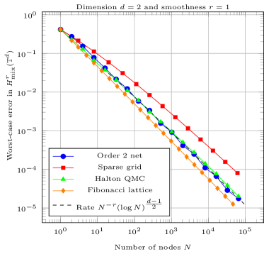
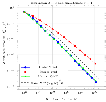
Figure 2: Worst-case errors of order 2 digital nets in $H^{r}_{\text{mix}}(\mathbb{T}^{d})$ for smoothness $r=1$.

6 Numerical experiments

In this section we use the theory of reproducing kernel Hilbert spaces (RKHS) to explicitly compute the worst-case error for particular constructions of order 2 digital nets based on Niederreiter-Xing sequences in the case of integer smoothness $r\in\{1,2\}$. Moreover, we give numerical examples for the case of fractional smoothness, i.e. $r=\frac{3}{2}$.

6.1 Worst-case errors in $\mathbf{H^{2}_{\text{mix}}(\mathbb{T}^{d})}$

Let us recall that the Besov space $S^{r}_{2,2}B(\mathbb{T}^{d})$ coincides with the classical tensor product Sobolev space $H^{r}_{\text{mix}}(\mathbb{T}^{d}):=H^{r}(\mathbb{T})\otimes\ldots\otimes H^{r}(\mathbb{T})$ of functions with mixed derivatives of order $r$ bounded in $L_{2}(\mathbb{T}^{d})$. Since for $r>1/2$ the space $H^{r}_{\text{mix}}(\mathbb{T}^{d})$ is a Hilbert space which is embedded in $C(\mathbb{T}^{d})$, it is well-known [2] that for a given choice of an inner product $\langle\cdot,\cdot\rangle_{H^{r}_{\text{{\rm mix}}}}$ there exists a symmetric and positive definite kernel $K:\mathbb{T}^{d}\times\mathbb{T}^{d}\rightarrow\mathbb{R}$ that reproduces point-evaluation, i.e., it holds $f(x)=\langle f(\cdot),K(\cdot,x)\rangle_{H^{r}_{\text{{\rm mix}}}}$ for all $x\in[0,1)^{d}$ and $f\in H^{r}_{\text{{\rm mix}}}(\mathbb{T}^{d})$. Then one can use the well-known worst-case error formula to compute the quantities

$$\|R_{N}|(H^{r}_{\text{mix}})^{*}\|^{2}= \sup_{\|f|H^{r}_{\text{mix}}\|\leq 1}\left|\int_{\mathbb{T}^{d}}f(x)\,dx-\sum_{i=1}^{N}\lambda_{i}f(x^{i})\right|^{2}$$ (6.1)

$$= \int_{\mathbb{T}^{d}}\int_{\mathbb{T}^{d}}K(x,y)\,\mathrm{d}x\mathrm{d}y-2\sum_{i=1}^{N}\lambda_{i}\int_{\mathbb{T}^{d}}K(x^{i},y)\,\mathrm{d}y+\sum_{i=1}^{N}\sum_{j=1}^{N}\lambda_{i}\lambda_{j}K(x^{i},x^{j})$$ (6.2)

explicitly, if a point set $\mathcal{P}_{N}=\{x^{1},\ldots,x^{N}\}$ of integration nodes and associated integration weights $\lambda_{1},\ldots,\lambda_{N}\in\mathbb{R}$ are given. In order to have a simple closed-form representation of the kernel $K$ we choose the inner product of the univariate Sobolev space $H^{r}(\mathbb{T})$ to be

$$\langle f,g\rangle_{H^{r}(\mathbb{T})}=\hat{f}(0)\,\overline{\hat{g}(0)}+\sum_{k\in\mathbb{Z}\setminus\{0\}}|2\pi k|^{2r}\hat{f}(k)\,\overline{\hat{g}(k)}.$$ (6.3)

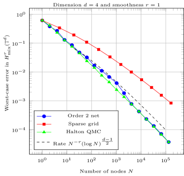
Figure 3: Worst-case errors of order 2 digital nets in $H^{r}_{\text{mix}}(\mathbb{T}^{d})$ for smoothness $r=1$.

The induced norm is given by

$$\|f\|_{H^{r}}^{2}=|\hat{f}(0)|^{2}+\sum_{k\in\mathbb{Z}\setminus\{0\}}^{\infty}|2\pi k|^{2r}\,|\hat{f}(k)|^{2}=\left|\int_{0}^{1}f(x)\,dx\right|^{2}+\int_{0}^{1}|f^{(r)}(x)|^{2}\,\mathrm{d}x,$$ (6.4)

where the last equality only holds for $r\in\mathbb{N}$. Then the reproducing kernel $K_{1}:\mathbb{T}\times\mathbb{T}\rightarrow\mathbb{R}$ of $H^{r}(\mathbb{T})$ is given by [57]

$$K_{1,r}(x,y):= 1+\sum_{k\in\mathbb{Z}\setminus\{0\}}|2\pi k|^{-2r}\exp(2\pi\mathrm{i}k(x-y))$$ (6.5)

$$= 1+2\sum_{k=1}^{\infty}|2\pi k|^{-2r}\cos(2\pi k(x-y))\,.$$

If $r\in\mathbb{N}$ the kernel can be written as

$$K_{1,r}(x,y)=1+\frac{(-1)^{r+1}}{(2r)!}B_{2r}(|x-y|),$$ (6.6)

where $B_{2r}:[0,1]\rightarrow\mathbb{R}$ denotes the Bernoulli polynomial of degree $2r$. Since $H^{r}_{\text{mix}}(\mathbb{T}^{d})$ is the tensor product of univariate Sobolev spaces, the reproducing kernel of $H^{r}_{\text{mix}}(\mathbb{T}^{d})$ is given by the product of the univariate kernels, i.e.

$$K_{d,r}(x,y)=\prod_{j=1}^{d}K_{1,r}(x_{j},y_{j}),\quad x,y\in\mathbb{T}^{d}$$

reproduces point evaluation in $H^{r}_{\text{mix}}(\mathbb{T}^{d})$.

As an example we employ order 2 digital nets that are based on Xing-Niederreiter sequences [37], which are known to yield smaller $t$-values than e.g. Sobol- or classical Niederreiter-sequences [12]. For the special case of rational places this construction was implemented by Pirsic [42], see also [13]. It is known [38] that one obtains a digital $(t,n,d)$-net from a digital $(t,n,d-1)$-sequence $\{x^{0},\ldots,x^{2^{n}-1}\}$ by adding an equidistant coordinate, i.e.

$$\{(\lfloor x^{i}_{1})\rfloor_{n},\ldots,\lfloor x^{i}_{d-1})\rfloor_{n},i/2^{n}):i=0,\ldots,2^{n}-1\},$$ (6.7)

where $\lfloor\cdot\rfloor_{n}$ denotes the $n$-th digit truncation.

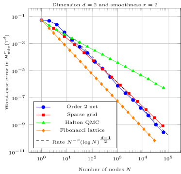
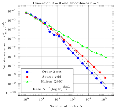
Figure 4: Worst-case errors for smoothness $r=2$ and various cubature methods.

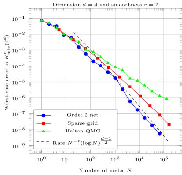
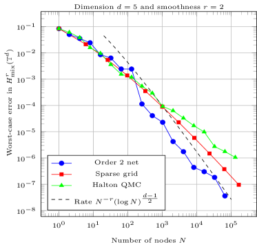
Figure 5: Worst-case errors for smoothness $r=2$ and various cubature methods.

So we first construct a classical (order 1) digital net from the Xing-Niederreiter sequence using the ’sequence-to-net’ propagation rule (6.7). Then we employ the digit interlacing operation (4.1) to obtain an order 2 net.

For this particular kernel and point set the formula for the squared worst-case error can be written as

$$\sup_{\|f|H^{r}_{\text{mix}}(\mathbb{T}^{d})\|\leq 1}\left|\int_{\mathbb{T}^{d}}f(x)\,dx-2^{-n}\sum_{i=0}^{2^{n}-1}f(x^{i})\right|^{2}=-1+2^{-2n}\sum_{i=0}^{2^{n}-1}\sum_{j=0}^{2^{n}-1}K_{d,r}(x^{i},x^{j}).$$ (6.8)

In Figures 2 and 3 we computed the worst-case errors of the described construction of an order 2 digital net in $H^{1}_{\text{mix}}(\mathbb{T}^{d})$ for dimensions $d=2,\ldots,5$ and compared it to the bounds from Theorem 5.3. These expected rates of convergence $N^{-r}(\log N)^{(d-1)/2}$ were plotted in dashed lines. One can see that our observed rate of convergence matches the predicted one even though a dimension-dependent constant seems to be involved. Additionally we computed the worst-case error for the Halton construction [23] which is amongst the most popular QMC sequences and performs very well for smoothness $r=1$. Moreover, we consider the sparse grid construction which consists of certain tensor products of the univariate trapezoidal rule, yielding an error decay of $\mathcal{O}(N^{-r}(\log N)^{(d-1)(r+\frac{1}{2})})$, see [20]. Sparse grids go back to ideas from Smolyak [45] and belong to today’s standard approaches when it comes to high-dimensional problems, see e.g. [5] and the references therein. It can be seen that their rate of convergence depends stronger on the dimension $d$ than the low-discrepancy approaches.

The same analysis was done for the case of second order smoothness in $H^{2}_{\text{mix}}(\mathbb{T}^{d})$. The results are given in Figures 4 and 5. Here, all quantities were computed in 128-bit floating point arithmetic. In the bivariate case it is known [48, 20] that the Fibonacci lattice performs asymptotically optimal. This can also be observed in Figures 2 and 4 where the Fibonacci lattice yields the same (optimal) rate of convergence as the order 2 digital nets, although it seems to have a significantly smaller constant. For small Fibonacci numbers, it is even known that the Fibonacci lattice is the globally optimal point set [26]. In summary, we can see that the order $2$ net, the Fibonacci lattice and the sparse grid are able to benefit from the higher order smoothness, while the Halton sequence does not improve over $N^{-1}(\log N)^{(d-1)/2}$.

6.2 Integration of kink functions

Mixed Sobolev regularity $H^{r}_{\text{{\rm mix}}}$ is often not suitable to reflect the correct asymptotical behavior of the integration error of one fixed function. In case of kink functions, like for instance the Faber hat functions $v_{j,k}$ from (3.2), we observe the Sobolev regularity $v_{j,k}\in H^{3/2-\varepsilon}$ whereas the Besov regularity is $B^{2}_{1,\infty}$. The tensor product kink functions belong to $H^{3/2-\varepsilon}_{\text{mix}}$, but as well to $S^{2}_{1,\infty}B$. This can be easily deduced from the characterization in Lemma 2.7. Glancing at Theorem 5.3, we see that the (optimal) error bound does not depend on the integrability parameter $p$ of the mixed Besov space $S^{r}_{p,q}B$. Hence, it seems to be reasonable to “sacrifice” integrability in order to gain smoothness which makes our Besov model more suitable for this issue. Our first example is a typical kink function of the form $g(x)=\max\{0,h(x)\}$. To be more precise, we consider tensor products of the univariate ( normalized) function

$$g(x)=\frac{15\sqrt{5}}{4}\max\left\{\frac{1}{5}-(x-1/2)^{2},0\right\},$$ (6.9)

which belongs to $B^{2}_{1,\infty}(\mathbb{T})$ and has integral $\int_{0}^{1}g(x)\,\mathrm{d}x=1$. Hence the tensor product function

$$g_{d}(x):=\prod_{j=1}^{d}g(x_{j})\quad,\quad x\in\mathbb{T}^{d}\,,$$ (6.10)

belongs to $S^{2}_{1,\infty}B(\mathbb{T}^{d})$ with integral $\int_{\mathbb{T}^{d}}g_{d}(x)\,dx=1$ and the same holds for the shifted functions

$$\tilde{g}_{d}(x,\eta):=\prod_{j=1}^{d}g(\mathrm{frac}(x_{j}+\eta_{j}))\quad,\,\quad x\in\mathbb{T}^{d}\,,$$ (6.11)

where $\mathrm{frac}(t)=t-\lfloor t\rfloor$ denotes the fractional part of $t$ and $\eta\in[0,1]^{d}$.

In order to obtain smooth convergence rates we compute the maximum error of $1000$ randomly shifted instances of $\tilde{g}_{d}$, i.e.

$$\tilde{R}_{N}(g)=\max_{k\in\{1,\ldots,1000\}}\left|\int_{\mathbb{T}^{d}}\tilde{g}_{d}(x,\eta^{k})\,\mathrm{d}x-\sum_{i=1}^{N}\lambda_{i}\tilde{g}_{d}(x^{i},\eta^{k})\right|\,.$$ (6.12)

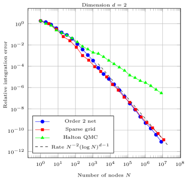
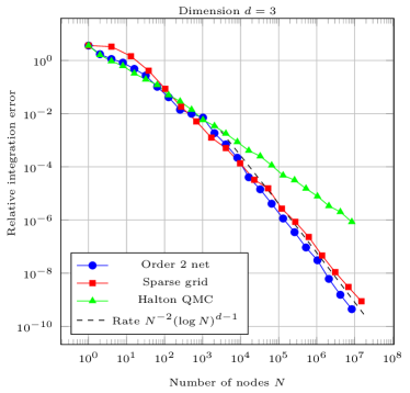
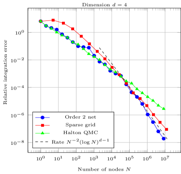
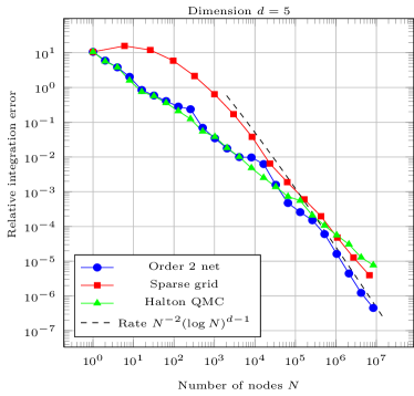
Figure 6: Maximum over the relative integration errors for the test function (6.11) with kinks.

Here, the shifts $\eta^{k}\sim\mathcal{U}[0,1]^{d}$ are independent and identically uniformly distributed in $\mathbb{T}^{d}$ for $k=1,\ldots,1000$ and the integration nodes $x^{i},i=1,\ldots,N$ and associated integration weights $\lambda_{i}$ depend on the chosen integration method and also the total number of function values $N$. The results are given in Figure 6, where we compared the performance of the order $2$ nets to both the sparse grid and Halton construction.

Next, we consider a toy example from $B^{3/2}_{1,\infty}(\mathbb{T})$ which has Sobolev regularity below $r=1$. We take the square root of the level $0$ hat function (3.2) normalized with respect to $L_{1}(\mathbb{T}^{d})$, i.e.,

$$g(t):=\frac{3}{\sqrt{2}}\sqrt{v_{0,0}(t)}\,.$$ (6.13)

It holds $\int_{\mathbb{T}}g(t)\,dt=1$. The Besov regularity $r=3/2$ can be easily deduced from Lemma 2.7. Hence the tensor product function

$$g_{d}(x):=\prod_{j=1}^{d}g(x_{j})\quad,\quad x\in\mathbb{T}^{d}\,,$$ (6.14)

belongs to $S^{3/2}_{1,\infty}B(\mathbb{T}^{d})$ with integral $\int_{\mathbb{T}^{d}}g_{d}(x)\,dx=1$. The same holds for the shifted functions

$$\tilde{g}_{d}(x,\eta):=\prod_{j=1}^{d}g(\mathrm{frac}(x_{j}+\eta_{j}))\quad,\quad x\in\mathbb{T}^{d}\,.$$ (6.15)

Again, we compute the maximum integration error of $1000$ shifted instances of $\tilde{g}$. The results are given in Figure 7. It can be clearly observed that the obtained convergence rates match the ones predicted in Theorem 5.3, i.e. $N^{-\frac{3}{2}}(\log N)^{d-1}$.

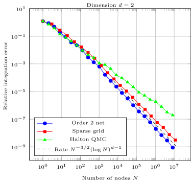
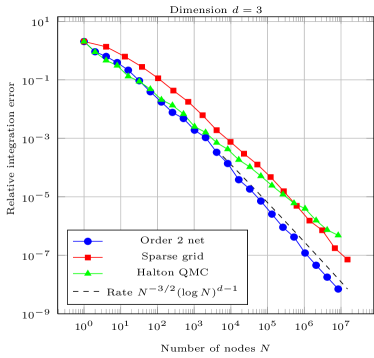
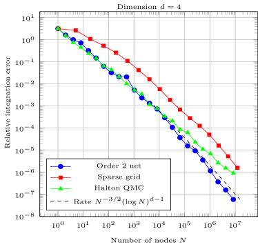
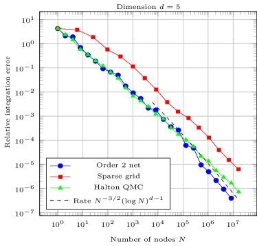
Figure 7: Maximum over the relative integration errors for the test function (6.15) with fractional smoothness $r=\frac{3}{2}$.

Acknowledgments The authors would like to thank the HCM Bonn and the organizers of the HCM-workshop Discrepancy, Numerical Integration, and Hyperbolic Cross Approximation where this work has been initiated. In addition, they would like to thank the organizers of the semester program High-Dimensional Approximation at ICERM, Brown University, for providing a pleasant and fruitful working atmosphere. Finally, they would like to thank Dinh Dũng, Michael Griebel, Winfried Sickel and Vladimir Temlyakov for several helpful remarks on earlier versions of this manuscript.

References

• [1] T. I. Amanov. Spaces of Differentiable Functions with Dominating Mixed Derivatives. Nauka Kaz. SSR, Alma-Ata, 1976.
• [2] N. Aronszajn. Theory of reproducing kernels. Trans. Amer. Math. Soc., 68:337–404, 1950.
• [3] N. S. Bakhvalov. Optimal convergence bounds for quadrature processes and integration methods of Monte Carlo type for classes of functions. Zh. Vychisl. Mat. i Mat. Fiz., 4(4):5–63, 1963.
• [4] D. Bilyk. On Roth’s orthogonal function method in discrepancy theory. Unif. Distrib. Theory, (6):143–184, 2011.
• [5] H.-J. Bungartz and M. Griebel. Sparse grids. Acta Numer., 13:1–123, 2004.
• [6] J. Dick. Explicit constructions of quasi-Monte Carlo rules for the numerical integration of high-dimensional periodic functions. SIAM J. Numer. Anal., 45:2141–2176, 2007.
• [7] J. Dick. Walsh spaces containing smooth functions and quasi-Monte Carlo rules of arbitrary high order. SIAM J. Numer. Anal., 46:1519–1553, 2008.
• [8] J. Dick. Discrepancy bounds for infinite-dimensional order two digital sequences over $\mathbb{F}_{2}$. J. Number Theory, 136:204–232, 2014.
• [9] J. Dick and P. Kritzer. Duality theory and propagation rules for generalized digital nets. Math. Comp., 79:993–1017, 2009.
• [10] J. Dick, F. Kuo, Q. Thong Le Gia, and C. Schwab. Multi-level higher order qmc galerkin discretization for affine parametric operator equations. ArXiv e-prints, June 2014.
• [11] J. Dick, Q. T. Le Gia, and C. Schwab. Higher order quasi-monte carlo integration for holomorphic, parametric operator equations. ArXiv e-prints, Sept. 2014.
• [12] J. Dick and H. Niederreiter. On the exact $t$-value of Niederreiter and Sobol’ sequences. J. Complexity, 24(5–6):572 – 581, 2008.
• [13] J. Dick and F. Pillichshammer. Digital nets and sequences. Discrepancy theory and quasi-Monte Carlo integration. Cambridge University Press, Cambridge, 2010.
• [14] J. Dick and F. Pillichshammer. Discrepancy theory and quasi-monte carlo integration. In Panorama in Discrepancy Theory. Springer–Verlag, 2013.
• [15] J. Dick and F. Pillichshammer. Explicit constructions of point sets and sequences with low discrepancy. In: Uniform distribution and quasi-Monte Carlo methods - Discrepancy, integration and applications, pages 63–86, 2014.
• [16] J. Dick and F. Pillichshammer. Optimal $L_{2}$-discrepancy bounds for higher order digital sequences over the finite field $\mathbb{F}_{2}$. Acta Arith., 162(1):65–99, 2014.
• [17] V. V. Dubinin. Cubature formulas for classes of functions with bounded mixed difference. Matem. USSR Sbornik, 76:283–292, 1993.
• [18] V. V. Dubinin. Cubature formulae for Besov classes. Izvestiya Math., 61(2):259–283, 1997.
• [19] D. Dũng. B-spline quasi-interpolant representations and sampling recovery of functions with mixed smoothness. J. Complexity, 27(6):541–567, 2011.
• [20] D. Dũng and T. Ullrich. Lower bounds for the integration error for multivariate functions with mixed smoothness and optimal Fibonacci cubature for functions on the square. Math. Nachr., DOI: 10.1002/mana.201400048.
• [21] G. Faber. Über stetige Funktionen. Math. Ann., 66:81–94, 1909.
• [22] P. Glasserman. Monte Carlo Methods in Financial Engineering. Applications of mathematics : stochastic modelling and applied probability. Springer, 2004.
• [23] J. H. Halton. Algorithm 247: Radical-inverse quasi-random point sequence. Commun. ACM, 7(12):701–702, Dec. 1964.
• [24] A. Hinrichs. Discrepancy of Hammersley points in Besov spaces of dominating mixed smoothness. Math. Nachr., 283(3):478–488, 2010.
• [25] A. Hinrichs. Discrepancy, integration and tractability. In J. Dick, F. Y. Kuo, G. W. Peters, I. H. Sloan, Monte Carlo and Quasi-Monte Carlo Methods 2012, 2014.
• [26] A. Hinrichs and J. Oettershagen. Optimal point sets for quasi–Monte Carlo integration of bivariate periodic functions with bounded mixed derivatives. to appear in Proc. conf. MCQMC Leuven, 2014.
• [27] E. Hlawka. Zur angenäherten Berechnung mehrfacher Integrale. Monatsh. Math., 66:140–151, 1962.
• [28] N. M. Korobov. Approximate evaluation of repeated integrals. Dokl. Akad. Nauk SSSR, 124:1207–1210, 1959.
• [29] H. N. L. Kuipers. Uniform distribution of sequences. John Wiley & Sons, Ltd., New York, 1974.
• [30] L. Markhasin. Discrepancy and integration in function spaces with dominating mixed smoothness. Dissertationes Math., 494:1–81, 2013.
• [31] L. Markhasin. Discrepancy of generalized Hammersley type point sets in Besov spaces with dominating mixed smoothness. Unif. Distr. Theory, 8(1):135–164, 2013.
• [32] L. Markhasin. Quasi-Monte Carlo methods for integration of functions with dominating mixed smoothness in arbitrary dimension. J. Complexity, 29(5):370–388, 2013.
• [33] L. Markhasin. ${L}_{2}$- and ${S}^{r}_{p,q}{B}$-discrepancy of (order 2) digital nets. Acta Arith., 168(2):139–160, 2015.
• [34] J. Matoušek. Geometric discrepancy. An illustrated guide. Springer-Verlag, Berlin, 1999.
• [35] V. K. Nguyen, M. Ullrich, and T. Ullrich. Boundedness of pointwise multiplication and change of variable and applications to numerical integration. Preprint, 2015.
• [36] H. Niederreiter. Point sets and sequences with small discrepancy. Monatsh. Math., 104:273–337, 1987.
• [37] H. Niederreiter and C. Xing. A construction of low-discrepancy sequences using global function fields. Acta Arith., 73(1):87–102, 1995.
• [38] H. Niederreiter and C. Xing. Low-discrepancy sequences and global function fields with many rational places. Finite Fields and Their Applications, 2(3):241 – 273, 1996.
• [39] S. M. Nikol’skij. Approximation of functions of several variables and embedding theorems. Nauka Moskva, 1977.
• [40] E. Novak. Some results on the complexity of numerical integration. In Monte Carlo and Quasi-Monte Carlo Methods, to appear in Proc. conf. MCQMC Leuven, 2014.
• [41] E. Novak and H. Woźniakowski. Tractability of multivariate problems. Volume II: Standard information for functionals, volume 12 of EMS Tracts in Mathematics. European Mathematical Society (EMS), Zürich, 2010.
• [42] G. Pirsic. A software implementation of Niederreiter-Xing sequences. In Monte Carlo and quasi-Monte Carlo methods 2000. Springer, Berlin, 2002.
• [43] H.-J. Schmeisser and H. Triebel. Topics in Fourier analysis and function spaces. A Wiley-Interscience Publication. John Wiley & Sons Ltd., Chichester, 1987.
• [44] M. M. Skriganov. Constructions of uniform distributions in terms of geometry of numbers. J. Complexity, 6:200–230, 1994.
• [45] S. Smolyak. Quadrature and interpolation formulas for tensor products of certain classes of functions. Dokl. Akad. Nauk SSSR, 4:240–243, 1963.
• [46] V. N. Temlyakov. On reconstruction of multivariate periodic functions based on their values at the knots of number-theoretical nets. Anal. Math., 12:287–305, 1986.
• [47] V. N. Temlyakov. On a way of obtaining lower estimates for the errors of quadrature formulas. Mat. Sb., 181(10):1403–1413, 1990.
• [48] V. N. Temlyakov. Error estimates for Fibonacci quadrature formulas for classes of functions with a bounded mixed derivative. Trudy Mat. Inst. Steklov., 200:327–335, 1991.
• [49] V. N. Temlyakov. Approximation of periodic functions. Computational Mathematics and Analysis Series. Nova Science Publishers Inc., Commack, NY, 1993.
• [50] V. N. Temlyakov. Cubature formulas, discrepancy, and nonlinear approximation. J. Complexity, 19(3):352–391, 2003. Numerical integration and its complexity (Oberwolfach, 2001).
• [51] H. Triebel. Bases in function spaces, sampling, discrepancy, numerical integration, volume 11 of EMS Tracts in Mathematics. European Mathematical Society (EMS), Zürich, 2010.
• [52] H. Triebel. Faber systems and their use in sampling, discrepancy, numerical integration. EMS Series of Lectures in Mathematics. European Mathematical Society (EMS), Zürich, 2012.
• [53] M. Ullrich and T. Ullrich. The role of Frolov’s cubature formula for functions with bounded mixed derivative. ArXiv e-prints, 2015. arXiv:1503.08846 [math.NA].
• [54] T. Ullrich. Function spaces with dominating mixed smoothness; characterization by differences. Jenaer Schriften zur Mathematik und Informatik, Math/Inf/05/06, 2006.
• [55] T. Ullrich. Smolyak’s algorithm, sampling on sparse grids and Sobolev spaces of dominating mixed smoothness. East J. Approx., 14(1):1–38, 2008.
• [56] T. Ullrich. Optimal cubature in Besov spaces with dominating mixed smoothness on the unit square. J. Complexity, 30:72–94, 2014.
• [57] G. Wahba. Smoothing noisy data with spline functions. Numer. Math., 24(5):383–393, 1975.