Propagation of a single hole defect in the one-dimensional Bose-Hubbard model

Abstract

We study nonequilibrium dynamics in the one-dimensional Bose-Hubbard model starting from an initial product state with one boson per site and a single hole defect. We find that for parameters close to the quantum critical point, the hole splits into a core showing a very slow diffusive dynamics, and a fast mode which propagates ballistically. Using an effective fermionic model at large Hubbard interactions $U$, we show that the ballistic mode is a consequence of an interference between slow holon and fast doublon dynamics, which occurs once the hole defect starts propagating into the bosonic background at unit filling. Within this model, the signal velocity of the fast ballistic mode is given by the maximum slope of the dispersion of the doublon quasiparticle in good agreement with the numerical data. Furthermore, we contrast this global quench with the dynamics of a single hole defect in the ground state of the Bose-Hubbard model and show that the dynamics in the latter case is very different even for large values of $U$. This can also be seen in the entanglement entropy of the time evolved states which grows much more rapidly in time in the global quench case.

I Introduction

An investigation of the states of matter and excitations of a quantum system is usually based on its dynamical response to external perturbations. This includes frequency-dependent response functions and scattering cross sections tested in condensed matter experiments,kittelbook ; ashcroftbook as well as time-dependent correlation functions measured in experiments on cold atomic gases.greiner2002 ; kinoshita2006 ; cheneau2012 ; fukuhara2013nat ; fukuhara2013nph ; hild2014 ; arxivxia ; bloch2008 The investigation of time-dependent correlation functions in and out of equilibrium has recently attracted renewed interest due to experiments on cold atomic gases in optical lattices which provide useful schemes for the preparation of quantum states and the tuning of interactions.bloch2008 ; paredes2004 ; kinoshita2004 Recent developments allow, in particular, for single-site addressability, both in preparation and detectiongericke2008 ; bakr2009 ; wuertz2009 ; sherson2010 ; endres2011 .

A lot of attention has been focussed on the dynamics of quasi one-dimensional systems where quantum fluctuations are strong and can prevent the ground state from attaining any type of long-range order. In this case, the system can often be described by Luttinger liquid (LL) theory giamarchibook , a hydrodynamic approach for the collective excitations (density fluctuations), which propagate with an interaction-dependent velocity. Recent studies, however, have shown that LL theory is not sufficient to fully describe the dynamics of such systems even at zero temperature. Nonlinearities of the dispersion have to be taken into account, which lead to x-ray edge-type singularities in response functions and new quasiparticles. An extension of standard LL theory, the so-called nonlinear Luttinger liquid (NLL) theory, has been developed, which is capable of describing the collective excitations and the new quasiparticles on an equal footing.imambekov2012 This allows, for example, to calculate the dynamical structure factor for the Lieb-Liniger modelliebliniger1963 —the continuum limit of the Bose-Hubbard model in the superfluid phase— which shows power-law singularities at the edges of its support.imambekov2012 Very recently, it has been demonstrated that the NLL approach can also be extended to small finite temperatures arxivkarrasch . One of the main findings of the latter study is that the combination of quantum and thermal fluctuations can dramatically alter the dynamical response compared to the zero temperature case. For the spin-1/2 XXZ chain, in particular, the autocorrelation function at finite temperature and long times was shown to exhibit a slow diffusive decay $\sim 1/\sqrt{t}$ in time $t$, explaining the diffusive response measured in NMR and $\mu$SR experiments sirker2009 ; sirker2011 ; thurber2001 . To also understand spin and energy transport in the linear response regime, one has to identify, in addition, all the local and quasilocal conserved charges of the microscopic model under consideration. For the XXZ chain, for example, the spin current is only partly conserved, so that a ballistic contribution coexists with a diffusive contribution.sirker2009 ; sirker2011 This result shows that even the linear response in a very simple strongly correlated one-dimensional quantum model can already be quite complicated and very different from phenomenological theories degennes1958 .

Dynamics and transport far from equilibrium are, on the other hand, much less understood so far even for the simplest interacting models. Much of the interest has concentrated on quantum quenches, i. e., the dynamics ensuing after preparing the system in the ground state of a Hamiltonian, and then suddenly changing one of its microscopic parameters. The expectation values of local observables at long times after the quench in a generic, infinitely large quantum system are expected to become time independent and to be described by a Gibbs ensemble.rigol2008 For integrable quantum systems, on the other hand, the additional local and quasilocal conserved charges have to be taken into account as well, leading to a generalized Gibbs ensemble rigol2007 ; fagotti2013 ; sirker2014 . While (generalized) Gibbs ensembles can help us to calculate the equilibrated values of local observables after a quantum quench for a system in the thermodynamic limit, they are not helpful in identifying the dominant relaxation processes and in describing the nonequilibrium dynamics itself. A notable known feature in the quench dynamics of a model with short-range interactions, starting from an initial state with a finite correlation length, is the existence of Lieb-Robinson bounds which state that correlations can only spread with a finite speed.lieb1972 ; bravyi2006 The emergence of an effective light cone has also been observed in experiments.cheneau2012 ; langen2013 Furthermore, such bounds can exist for finite-temperature initial states as well.bonnes2014

A possible way to systematically probe nonequilibrium dynamics and transport beyond linear response is to consider local perturbations.kollath2005 ; kleine2008 ; langer2009 ; langer2011 ; fukuhara2013nph ; fukuhara2013nat ; karrasch2014 The advantage of this approach is that local perturbations can easily be created in an experimental setup of cold atoms, and that one can follow their evolution in time by measuring one-point functions instead of two-point correlators. For the Bose-Hubbard model, for example, the time evolution of local Gaussian density perturbations on top of the ground state has been studied by numerical density matrix renormalization group (DMRG) methods.kollath2005 In this work, it has been shown that for weak and intermediate interactions, small density perturbations travel through the system at a velocity which is consistent with the sound velocity in the corresponding continuum, exactly solvable Lieb-Liniger model. The expansion of density-wave packets in the one-dimensional Bose-Hubbard model has also been studied experimentally in an out-of-equilibrium situation.ronzheimer2013 Here, a gas of ³⁹K atoms was prepared in a harmonic confinement. The confinement was then lowered so that the atoms started to expand into the empty optical lattice. A slowing down of the expansion of the cloud was observed near the critical point in the ground state phase diagram. The same experiment in two dimensions showed, in addition, a separation of the cloud into a diffusive core and a background which spreads ballistically. An important feature of such expansion dynamics is that more than one velocity can be present due to the formation of bound states. Examples for such behavior are the XXZ model at large repulsive nearest-neighbor interactionganahl2012 ; fukuhara2013nat ; alba2013 ; liu2014 , as well as the Bose-Hubbard model, where the onsite repulsive interaction can lead to effectively bound states of doublons.jreissaty2013 ; degliespostiboschi2014

In this paper, we will study the non-equilibrium dynamics of one of the simplest local perturbations: a single hole defect in an initial product state with one boson per lattice site under the unitary time evolution of a Bose-Hubbard Hamiltonian. This setup can easily be realized using cold atomic gases, which offer single-site addressability in the preparation of initial states and in the detection of bosons after a quantum quench.gericke2008 ; bakr2009 ; wuertz2009 ; sherson2010 ; endres2011 Here, the hole defect spreads into a background which itself displays nontrivial dynamics, contrasting our setup from the case of an expansion into an empty lattice, which has been studied thoroughly for the bosonicrodriguez2006 ; jreissaty2011 ; muth2012 ; ronzheimer2013 ; jreissaty2013 ; vidmar2013 ; degliespostiboschi2014 and fermionicheidrichmeisner2009 ; kajala2011 ; karlsson2011 ; schneider2012 ; langer2012 versions of the Hubbard model. We will show, in particular, that the defect will either spread ballistically through the lattice or separate into a diffusive core coexisting with a fast ballistic mode, depending on the strength of the Hubbard interaction $U$. This phenomenon is reminiscent of the coexistence of ballistic and diffusive transport in the XXZ model at finite temperature, however, here it is not related to local or quasilocal conserved charges, but is rather, as we will show, a consequence of an interference effect between slow holon and fast doublon quasiparticle dynamics.

Our paper is organized as follows: In Sec. II we define the model, the initial states, and the time-dependent correlation functions which we study in the following. In Sec. III we explain the numerical method used to simulate the quench dynamics and introduce an effective fermionic modelbarmettler2012 to approximate the dynamics for large interactions. In Sec. IV we present the results of the numerical calculations and analyze these results using the effective fermionic model. In Sec. V we summarize our main results and discuss some of the remaining open questions.

II Model

We consider the one-dimensional Bose-Hubbard model,

$$H =J\sum_{j}(b_{j}^{\dagger}b_{j+1}+h.c.)+\frac{U}{2}\sum_{j}n_{j}(n_{j}-1),$$ (1)

where $b_{j}^{\dagger}$ ($b_{j}$) creates (annihilates) a boson at site $j$, $n_{j}=b_{j}^{\dagger}b_{j}$ is the local density operator, $U$ is the strength of the on-site repulsive interaction, and in the following, we set $J=1$. At unit filling, this model exhibits a quantum phase transition at $U_{c}\approx 3.37$ between a superfluid and a Mott insulating state.kuehner1998 We are interested in the time-dependent density profile $C_{r}(j,t)$ after removing a single particle at the center of the chain from a prepared uniform initial state $|\Psi_{r}\rangle$

$$C_{r}(j,t) =\langle\Psi_{r}|b_{j=0}^{\dagger}e^{iHt}n_{j}e^{-iHt}b_{j=0}|\Psi_{r}\rangle.$$ (2)

Our main focus is on the time evolution starting from the initial product state $|\Psi_{r\equiv p}\rangle\equiv\prod_{j}b_{j}^{\dagger}|0\rangle$. To understand the unique features of the non-equilibrium dynamics, we will compare our results with the equilibrium correlation function obtained by using the ground state $|\Psi_{r\equiv g}\rangle$ of the time-evolving Hamiltonian $H$ at unit filling as the initial state in Eq. (2). Alternatively, the latter case can be viewed as a local quench—defined as a local modification of the Hamiltonian or the initial state—while in the former case, an additional global quench from the ground state at infinite repulsion is performed.

III Method

III.1 Numerics

We calculate the correlation function (2) using the light cone renormalization group (LCRG) algorithm.enss2012 This algorithm is based on the time-dependent DMRGwhite1992 ; vidal2004 ; white2004 ; daley2004 and yields results directly in the thermodynamic limit. In our simulations we restrict the maximum number of bosons per lattice site to $5$ for $U\leq 6$, and to $3$ for $U>6$. By comparing with simulations where the maximum number of bosons is smaller we make sure that the results are converged on the scale of the figures we present in the following. Furthermore, we make sure that the discarded weight in each renormalization group step is smaller than $10^{-8}$. For the simulation times shown, this requires to increase the number of states kept in the truncated Hilbert space up to $8\,000$.

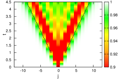
Figure 1: (Color online) The density profile $C_{p}(j,t)=1-\mathcal{J}_{j}^{2}(2t)$ for $U=0$ and $U=\infty$. The dashed lines show the linear spreading of the defect density, $j=\pm vt$, with a defect velocity $v=2$.

For the calculations where the initial state is the ground state $|\Psi_{g}\rangle$, we first perform an imaginary time evolution with the correct chemical potential $\mu$ to project an arbitrary starting vector onto the ground state at unit filling. The chemical potential is required because a canonical simulation in the thermodynamic limit is impossible. We check that $|\langle\Psi_{g}|n_{j}|\Psi_{g}\rangle-1|<10^{-6}$, i. e. we ensure convergence in the density to more than 6 digits.

III.2 Analytical results and approximations

The Bose-Hubbard model, Eq. (1), has two integrable limits: the limit of free bosons, $U=0$, and the limit of hard-core bosons, $U=\infty$. In both cases, we are dealing with single-particle dynamics and the density profile can be calculated exactly:

$$C_{p}^{U=0}(j,t)=C_{p}^{U=\infty}(j,t)=1-\mathcal{J}_{j}^{2}(2t),$$ (3)

where $\mathcal{J}_{j}$ is the $j$th Bessel function of the first kind. The density profile for these cases is shown in Fig. 1: The defect density spreads in a light cone with a velocity $v=2$. If we create a doublon instead of a hole defect, i.e., interchange $b_{j=0}^{\dagger}\leftrightarrow b_{j=0}$ in Eq. (2), the corresponding correlation function $\widetilde{C}_{p}$ is given by $\widetilde{C}_{p}^{U=0}(j,t)=1+\mathcal{J}_{j}^{2}(2t)$ and $\widetilde{C}_{p}^{U=\infty}(j,t)=1+\mathcal{J}_{j}^{2}(4t)$. In this case, the velocity of the expansion is given by $v=2$ for $U=0$ and $v=4$ for $U=\infty$. The by a factor of $2$ larger velocity in the latter case is a consequence of the Bose factor.

In the following, we will call any dynamics similar to the one shown in Fig. 1 ballistic. For a more precise definition, we follow Refs. langer2009, ; vidmar2013, and consider

$$R^{2}(t) =\sum_{j=-\infty}^{\infty}j^{2}(1-C_{p}(j,t)),$$ (4)

where $R(t)$ is a weighted measure for the distance over which the defect density has spread at time $t$. For the free and hardcore boson cases, the sum can be calculated exactly, using Eq. (3) and a standard identity for Bessel functions, resulting in

$$R^{2}(t) =\sum_{j=-\infty}^{\infty}j^{2}\mathcal{J}_{j}^{2}(2t)=2t^{2}.$$ (5)

The functional dependence of $R^{2}$ on time is thus the same as for a linearly dispersing, ballistic particle,

$$R^{2}(t) =\sum_{j=-\infty}^{\infty}\frac{j^{2}}{2}\left[\delta(j+vt)+\delta(j-vt)\right]=v^{2}t^{2}.$$ (6)

For large but finite $U$, an exact solution is not possible. Since high occupancies are suppressed, we can, however, approximate the dynamics in this limit by restricting the local Hilbert space to three states only: $|0\rangle_{j}$, $|1\rangle_{j}$, and $|2\rangle_{j}$. We can now interpret the state $|1\rangle_{j}$ as the vacuum, the doublon state $|2\rangle_{j}$ as a spin-up particle, and the holon state $|0\rangle_{j}$ as a spin-down particle. This is made explicit by the mapping

$$b_{j}=\sqrt{2}\,\widetilde{b}_{j\uparrow}+\widetilde{b}_{j\downarrow}^{\dagger}$$ (7)

where $\widetilde{b}_{j\sigma}$ are hardcore bosons.barmettler2012 The hardcore constraint for identical particles can be fulfilled by a second mapping onto fermions

$$\widetilde{b}_{j\uparrow}=Z_{j}c_{j\uparrow}\quad,\quad\widetilde{b}_{j\downarrow}=Z_{j}e^{i\pi n_{j\uparrow}}c_{j\downarrow}^{\dagger},$$ (8)

where $Z_{j}=\prod_{j^{\prime}<j}e^{i\pi\sum_{\sigma}n_{j\sigma}}$ is a Jordan-Wigner string, $c_{j\sigma}$ are fermionic operators, and $n_{j\sigma}=c^{\dagger}_{j\sigma}c_{j\sigma}$. Applying both transformations maps the bosonic Hamiltonian (1) in the restricted Hilbert space onto the fermionic Hamiltonian in momentum space,

$$H = \sum_{k\sigma}E_{k\sigma}c_{k\sigma}^{\dagger}c_{k\sigma}+i\sum_{k}\Delta_{k}(c_{k\uparrow}^{\dagger}c_{\bar{k}\downarrow}^{\dagger}-c_{\bar{k}\downarrow}c_{k\uparrow})$$ (9)

$$+ \frac{V}{N}\sum_{k,k^{\prime},q}c^{\dagger}_{k\uparrow}c_{k-q\uparrow}c^{\dagger}_{k^{\prime}\downarrow}c_{k^{\prime}+q\downarrow}$$

with $V\to\infty$. Here, we have defined $\bar{k}\equiv-k$, $\Delta_{k}=2\sqrt{2}\sin k$, and $E_{k\sigma}=U/2-(3+\sigma)\cos k$, where $\sigma=\pm 1$ for the spin-up and spin-down dispersions, respectively. The infinite potential $V$ projects out the unphysical state $|\!\!\uparrow\downarrow\rangle_{j}$, i.e., the state in which a doublon and a holon are on the same site. Within the truncated local Hilbert space, this transformation is exact.

As a further approximation, we will ignore the constraint and allow for double occupancies by setting $V=0$, leading to the unconstrained fermion (UF) model considered in Ref. barmettler2012, . This is justified as long as the density of doublons and holons is low, which is, at large enough interaction $U$, the case both for the ground state and the dynamics starting from the product state. The Hamiltonian, Eq. (9), can then be diagonalized by a Bogoliubov transformation,

$$c_{k\sigma} =\gamma_{k\sigma}\cos\theta_{k}+i\gamma_{\bar{k}\bar{\sigma}}^{\dagger}\sin\theta_{k},$$ (10)

with Bogoliubov angle $\theta_{k}=\arctan[2\Delta_{k}/(E_{k\uparrow}+E_{k\downarrow})]/2$. This leads to a diagonal Hamiltonian in the Bogoliubov quasiparticles, $H=\sum_{k\sigma}\epsilon_{k\sigma}\gamma_{k\sigma}^{\dagger}\gamma_{k\sigma}$, with dispersions

$$\epsilon_{k\sigma} =\frac{1}{2}\sqrt{(E_{k\uparrow}+E_{k\downarrow})^{2}+4\Delta_{k}^{2}}+\frac{\sigma}{2}(E_{k\uparrow}-E_{k\downarrow}).$$ (11)

The ground state $|\Psi_{g}\rangle$ of the Bose-Hubbard model (1) is then approximated by the vacuum of the $\gamma$-quasiparticles, $\gamma_{k\sigma}|\Psi_{g}\rangle\equiv 0$, while the product state $|\Psi_{p}\rangle$ takes the form of a BCS state,

$$|\Psi_{p}\rangle=\prod_{k}\left(\cos\theta_{k}+i\sin\theta_{k}\gamma_{k\uparrow}^{\dagger}\gamma_{\bar{k}\downarrow}^{\dagger}\right)|\Psi_{g}\rangle.$$ (12)

Note that the doublon quasiparticle dispersion becomes gapless at $U=8$, $\epsilon_{0\uparrow}=0$, showing that the UF approximation breaks down for smaller interactions. Instead of setting $V=0$ in Eq. (9), the constraint can be taken into account approximately by a summation of ladder diagrams which leads to a Bethe-Salpeter equation.kotov1998 The corresponding self-energies will then shift both quasiparticle dispersions $\epsilon_{k\sigma}$ up, so that the model remains stable even below $U=8$. However, this formalism cannot directly be used to calculate the nonequilibrium correlation function we are interested in. We will therefore only use the UF model to explain qualitative features of the defect dynamics for interactions $U\geq 8$.

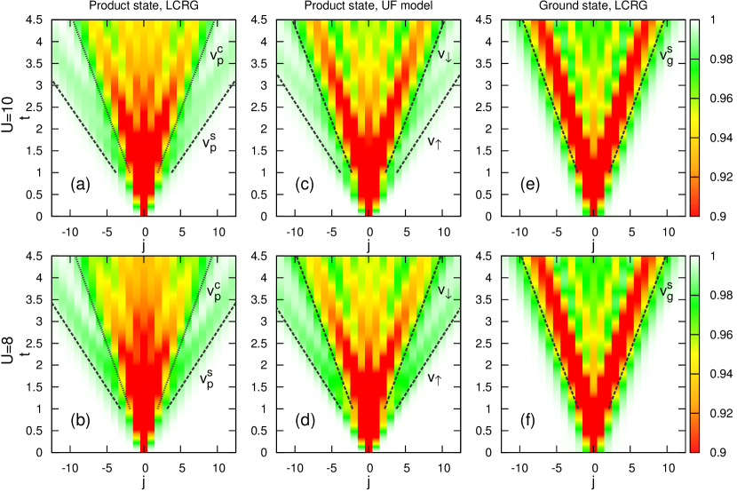
Figure 2: (color online) Density profiles $C_{p/g}(j,t)$ for large $U$: (a,b) Numerical results by LCRG for the initial product state $|\Psi_{p}\rangle$. (c,d) Results for the product state by numerically evaluating the integrals (IV.1) in the UF model approximation. (e,f) LCRG results with the ground state $|\Psi_{g}\rangle$ as initial state. The dashed lines in (a,b) and (e,f) denote the numerically extracted velocities $v_{p}^{s}$ and $v_{g}^{s}$, respectively. The dotted lines in (a,b) are a guide to the eye indicating the slow core velocity $v_{p}^{c}$. The dashed lines in (c,d) denote the velocities $v_{\sigma}$ defined in Eq. (14).

IV Results

IV.1 Large interactions

In Fig. 2 (a) and (b), we show the numerically obtained profiles $C_{p}(j,t)$ for large, but finite values of the interaction strength. In both cases, a clear qualitative change as compared to the $U=\infty$ case shown in Fig. 1 is observed. Instead of a ballistic spreading with a single velocity, we find a separation into a central light cone spreading with velocity $v_{p}^{c}$, and an extra contribution which moves with a faster velocity $v_{p}^{s}$ and clearly separates itself from the main defect density. To extract the Lieb-Robinson velocity of the first signal, $v_{p}^{s}$, from the numerical data, we take the point $j(t)$ where the defect density has reached half of the height of the first peak of its time-dependent distribution as reference point, and perform a linear fit according to $j(t)=v_{p}^{s}t$.enss2012

Next, we show that the presence of two velocities in the defect dynamics can be explained using the effective UF model. Expressing the bosonic density operator in the restricted Hilbert space in terms of the fermions, $n_{j}=1+c_{j\uparrow}^{\dagger}c_{j\uparrow}-c_{j\downarrow}^{\dagger}c_{j\downarrow}$, the correlation function $C_{p}$ can be calculated within the UF model approximation, see Appendix A for details. We obtain

$$C_{p}(j,t)=1-\bigg{|}\frac{1}{2\pi}\int_{-\pi}^{\pi}dk\,e^{ikj}\big{(}g_{k\downarrow}(t)\cos^{2}\theta_{k}+g_{k\uparrow}(t)\sin^{2}\theta_{k}\big{)}\bigg{|}^{2}-\bigg{|}\frac{1}{2\pi}\int_{-\pi}^{\pi}dk\,e^{ikj}\cos\theta_{k}\sin\theta_{k}\big{(}g_{k\downarrow}(t)-g_{k\uparrow}(t)\big{)}\bigg{|}^{2}$$

$$\approx 1-\mathcal{J}_{j}^{2}(2t)\left(1-\frac{2j(j-2)}{U^{2}t^{2}}\right)-\frac{1}{U^{2}}\left[\frac{j^{2}}{2t^{2}}\mathcal{J}_{j}^{2}(4t)-\mathcal{J}_{j}(2t)\left(\frac{j(j+1)}{t^{2}}\mathcal{J}_{j}(4t)+\frac{8}{t}\mathcal{J}_{j+1}(2t)-\frac{4}{t}\mathcal{J}_{j+1}(4t)\right)\right]$$ (13)

with propagators $g_{k\sigma}(t)\equiv\langle\gamma_{k\sigma}(t)\gamma_{k\sigma}^{\dagger}(0)\rangle=e^{-i\epsilon_{k\sigma}t}$, and we have performed the continuum limit. In the second line the integrals have been evaluated within an expansion in $1/U$ up to order $U^{-2}$. The result shows that contributions propagating with two different velocities as well as interference terms are present in the dynamics. The two different velocities can be determined from the maximal slope of the two dispersion relations,

$$v_{\sigma}=\max_{k}\,\frac{\partial\epsilon_{k\sigma}}{\partial k}.$$ (14)

From the $1/U$-expansion in Eq. (IV.1) we see that $v_{\uparrow}\to 4$ and $v_{\downarrow}\to 2$ for $U\to\infty$. This is consistent with the discussion of the holon and doublon dynamics at $U=\infty$ in Sec. III.2.

While the density profiles for the UF model, Fig. 2 (c) and (d), quantitatively differ from the LCRG results, they clearly show the same qualitative features. In particular, we find good agreement between the renormalized holon velocity and the slow core velocity, $v_{\downarrow}\approx v_{p}^{c}$, and the renormalized doublon velocity clearly determines the velocity of the first signal, $v_{\uparrow}\approx v_{p}^{s}$. In Fig. 3 we show the contributions to $C_{p}$, Eq. (IV.1), which contain the doublon propagator $g_{k\uparrow}$, separately. Comparing with Fig. 2 (a) and (b) we see that these contributions are indeed responsible for the fast mode. From the analytical result in the $1/U$-expansion, see second line in Eq. (IV.1), we can infer the weight $W$ of these contributions to leading order,

$$W \approx\sum_{j=-\infty}^{\infty}\frac{2j(j-2)}{U^{2}t^{2}}\mathcal{J}_{j}^{2}(2t)=\frac{4}{U^{2}}.$$ (15)

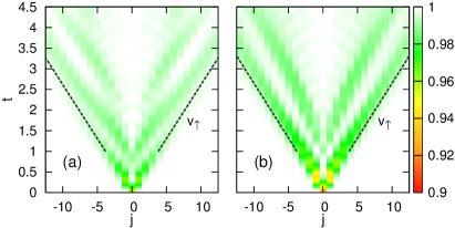
Figure 3: (color online) Contributions to $C_{p}(j,t)$ containing the $g_{k\uparrow}$ propagator, see Eq. (IV.1), for (a) $U=10$ and (b) $U=8$.

Another way to see that the mixing of holon and doublon excitations is responsible for the fast mode is to compare with the ground state correlation function $C_{g}$, shown in Fig. 2 (e) and (f), where the fast mode is absent, and only a single velocity $v_{g}^{s}$ can be observed. Within the UF model the initial state is now the vacuum of the $\gamma$-quasiparticles. From Eqs. (8) and (10) one immediately sees that in this case the $g_{k\uparrow}$ propagator does not show up in the correlation function $C_{g}$; accordingly, we see that $v_{g}^{s}\approx v_{\downarrow}$. The density profile therefore evolves differently in time, as is exemplarily shown in Fig. 4, where cuts of the density profiles for fixed times for the correlation functions $C_{p}$ and $C_{g}$ are compared. The difference in the defect dynamics starting from the ground state as opposed to the product state is also clearly seen in the entanglement entropy, $S_{\textrm{ent}}(t)$, between two halves of the infinite chain where the defect initially sits at the boundary, see Fig. 5. The extraction of a particle from the ground state of the system constitutes a local quench. In this case the entanglement entropy grows very slowly in time and the numerical simulation can be performed for long times.halimeh2014 For the initial product state, however, in addition to the local quench, a global quench is performed, because the initial product state $|\Psi_{p}\rangle$ only becomes the exact ground state at $U=\infty$. Hence, we see the well-known behavior for a global quench of the entanglement entropy increasing quickly and linearly with time.lieb1972 ; calabrese2005

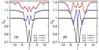
Figure 4: (color online) LCRG results for $U=8$: (a) $C_{p}(j,t)$ compared to (b) $C_{g}(j,t)$. In (a) the position of the fast mode is marked by arrows. Subsequent curves are shifted by $0.1$.

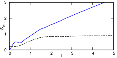
Figure 5: (color online) Entanglement entropy $S_{\textrm{ent}}(t)$ for $U=10$ between two halves of the infinite chain where the defect initially sits at the boundary. The solid line shows the linear increase of $S_{\textrm{ent}}(t)$ for the defect in the initial product state $|\Psi_{p}\rangle$, as expected for a global quench, while the dashed line represents the much slower increase of $S_{\textrm{ent}}(t)$ for the defect in the initial ground state $|\Psi_{g}\rangle$ (local quench).

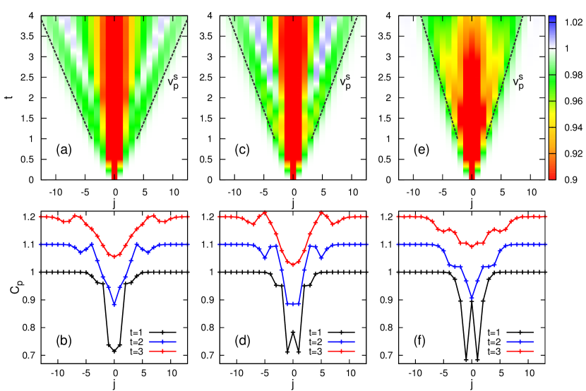
Figure 6: (color online) Density profiles $C_{p}(j,t)$ at weak and intermediate interactions for (a,b) $U=4.5$, (c,d) $U=3.0$, and (e,f) $U=1.5$. The dashed lines in (a,c,e) are the signal velocities $v_{p}^{s}$ as extracted from the numerical data. In (b,d,f) subsequent curves are shifted by $0.1$.

IV.2 Intermediate and weak interaction

For interaction strengths $U<8$ we can no longer use the UF model and have to fully rely on numerical results. From the numerical data shown in Fig. 6 (a-d), we see that the separation between the fast mode and the core becomes even more pronounced for intermediate interaction strengths. Particularly interesting is the case $U=3$, shown in Fig. 6 (c,d), where the core is almost frozen in and separated from the fast mode by a region where the density is even larger than one. While the fast mode still spreads ballistically, we can no longer assign a velocity to the core region, hinting at diffusive transport. The dynamics is thus very different from that of a defect in the ground state, shown in Fig. 7, which remains purely ballistic. For even smaller $U$, shown in Fig. 6 (e,f), the signal velocity $v_{p}^{s}$ decreases further so that a separation from a core region can no longer be resolved, at least not on the numerically accessible time scales. Eventually, purely ballistic dynamics is restored at $U=0$, where the density profile is again given by Eq. (3), see Fig. 1.

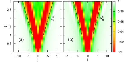
Figure 7: (Color online) Density profiles $C_{g}(j,t)$ starting from the ground state $|\Psi_{g}\rangle$ for (a) $U=4.5$, and (b) $U=3$. The dashed lines indicate the extracted signal velocities $v_{g}^{s}$.

To quantify this change in the expansion dynamics of the defect for the product state $|\Psi_{p}\rangle$, we calculate $R^{2}(t)$, as defined in Eq. (4). The results for various values of $U$ are shown in Fig. 8(a).

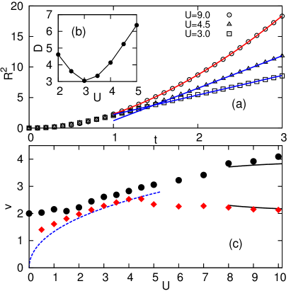
Figure 8: (color online) (a) $R^{2}(t)$ for the spreading of the defect with $|\Psi_{p}\rangle$ as initial state (symbols), a quadratic fit for $U=9$ (red line), and linear fits for $U=4.5$ and $U=3$ (blue lines). (b) Diffusion constants, $R^{2}(t)\sim Dt$, in the regime where the dynamics is dominantly diffusive at intermediate times. The expansion is slowest close to the critical point $U_{c}\approx 3.37$. (c) Velocity $v_{p}^{s}$ for the fastest signal in the product state dynamics (black circles), compared to the velocity of the signal $v_{g}^{s}$ for the ground state dynamics (red diamonds). For $U\geq 8$ both velocities are well approximated by the UF model velocities $v_{\uparrow}$ and $v_{\downarrow}$, Eq. (14), respectively (black solid lines). The blue dashed line denotes the sound velocity $v_{\textrm{LL}}$ in the Lieb-Liniger model.

At short times $t\lesssim 1$ we see that the dynamics is almost independent of the interaction strength and the defect spreads ballistically, $R^{2}\sim t^{2}$. At longer times there is a clear difference between large and intermediate $U$ values. While for $U=9$ the dynamics is also ballistic at intermediate times according to this criterion, the curves for $U=4.5$ and $U=3$ become linear, $R^{2}\sim Dt$, indicating a dominantly diffusive spreading of the defect at this time scale with a diffusion constant $D$.langer2009 ; vidmar2013 At these intermediate timescales we can extract the diffusion constant $D$ by linear fits; the results are shown in Fig. 8(b). We see that the spreading of the core depends on interaction strength $U$ and is slowest for values close to the critical point $U_{c}\approx 3.37$ which separates the superfluid from the Mott insulating regime in the ground state phase diagram. A similar slowing down near a critical point was also observed in the free expansion dynamics of a product state into an empty lattice,ronzheimer2013 ; vidmar2013 as well as in the non-equilibrium dynamics of the XXZ chain.barmettler2009 ; barmettler2010 Note, however, that the coexistence of diffusive and ballistic transport, which is clearly seen in Fig. 6 (a)-(d), cannot be resolved by the simple quantity $R^{2}(t)$ on intermediate timescales. In addition, $R^{2}(t)$ will always be dominated by a ballistic contribution in the long-time limit, no matter how small this contribution is.

A comparison of the different velocities observed in the dynamics of a single defect is shown in Fig. 8(c). In contrast to the diffusive core, critical slowing down is not observed in the velocity of the fast ballistic mode, $v_{p}^{s}$. Instead, the velocity $v_{p}^{s}$ is a monotonously increasing function in $U$ with $v_{p}^{s}=2$ at $U=0$, eventually approaching the value $v_{p}^{s}\to 4$ for large $U$ as expected for a single doublon in the initial product state, see Sec. III.2. For $U\geq 8$, $v_{p}^{s}$ is well approximated by the doublon quasiparticle velocity $v_{\uparrow}$ determined from the UF model. On the other hand, the velocity $v_{g}^{s}$ for the first front of the correlation function $C_{g}$ is not monotonous: Here we have $v_{g}^{s}(U=\infty)=2$, and the velocity first increases with decreasing $U$ and approximately agrees with the holon quasiparticle velocity $v_{\downarrow}$, see Eq. (14), in the regime where the UF approximation is valid. For smaller values of $U$, $v_{g}^{s}$ decreases with decreasing $U$. In the superfluid regime, we can then compare $v_{g}^{s}$ with the sound velocity of the corresponding continuum Lieb-Liniger model,calabrese2006 ; laeuchli2008

$$v_{\textrm{LL}}=\sqrt{U\left(2-\sqrt{\frac{U}{2\pi^{2}}}\right)}.$$ (16)

One has to keep in mind, however, that removing a particle from the ground state is not a low energy excitation of the system, but rather involves all momentum modes, $b_{j=0}=N^{-1}\sum_{k}b_{k}$. Only for sufficiently large $U$ in the superfluid regime, where the linearization of the spectrum is a good approximation for a large region around $k=0$, can we expect that both velocities are similar. This is indeed the case, as seen in Fig. 8(c). We find, furthermore, that the two velocities are also similar for $U$ values even slightly above the Mott transition. Here the excitation gap is relatively small so that the linear approximation of the dispersion still works approximately for a large range of momenta $k>0$.

V Summary and Conclusions

We have considered one of the simplest setups to systematically study the non-equilibrium dynamics of the one-dimensional Bose-Hubbard model: a single hole defect in an otherwise uniform state. If this initial state is a product state at unit filling, we have shown that the defect separates into a fast ballistic mode and a slower core. This behavior, which exists for any finite interaction, can be explained by an effective model valid for large values of $U$: doublon quasiparticles give rise to it. Using the quantity $R^{2}(t)$, which characterizes the extent of the region over which the defect has spread, we found that the core shows signs of a diffusive time evolution at intermediate interactions, leading to a coexistence of ballistic and diffusive defect dynamics. While the diffusive core shows critical slowing down, i. e. the dynamics is slowest close to the quantum critical point, the velocity of the fast mode does not. An effective theory which describes the coexistence of a diffusive core and the ballistic background in the dynamics and explains the slowing down of the diffusion near the quantum critical point remains as an open problem. We showed, furthermore, that the diffusive spreading of the defect only occurs when starting from the product state. If one considers instead the ground state of the Bose-Hubbard model as the initial state, then the dynamics is always purely ballistic, and the velocity in the superfluid regime is, for $U\gtrsim 1$, well described by the sound velocity of the Lieb-Liniger model. The proposed quench protocol can easily be implemented in an ultracold atom experiment using state-of-the-art preparation and detection techniques with single-site resolution and offers a systematic way to study the dynamics of local perturbations in the Bose-Hubbard model beyond the linear response regime. Importantly, this test of the non-equilibrium dynamics only requires to measure one-point correlation functions, because translational invariance of the initial state is broken by the defect.

Appendix A Density profile from the UF model

Our objective is to calculate the correlation function

$$C_{p}(j,t)=\langle\Psi_{p}|b_{0}^{\dagger}e^{iHt}n_{j}e^{-iHt}b_{0}|\Psi_{p}\rangle$$ (17)

within the approximation of the UF model. Using equations (7), (8), (10), and (12), we can express the initial state and the bosonic density operator, $n_{j}=1+c_{j\uparrow}^{\dagger}c_{j\uparrow}-c_{j\downarrow}^{\dagger}c_{j\downarrow}$, in terms of the $\gamma$-quasiparticles,

$$b_{0}|\Psi_{p}\rangle = \frac{1}{\sqrt{N}}\sum_{q}\gamma_{\bar{q}\downarrow}^{\dagger}\prod_{p\not=q}\left(\cos\theta_{p}+i\sin\theta_{p}\gamma_{p\uparrow}^{\dagger}\gamma_{\bar{p}\downarrow}^{\dagger}\right)|0_{\gamma}\rangle,$$ (18)

$$n_{j} = \frac{1}{N}\sum_{k,k^{\prime}}e^{i(k-k^{\prime})j}\left[\cos(\theta_{k}-\theta_{k^{\prime}})(\gamma_{k\uparrow}^{\dagger}\gamma_{k^{\prime}\uparrow}+\gamma_{\bar{k}\downarrow}\gamma_{\bar{k}^{\prime}\downarrow}^{\dagger})+i\sin(\theta_{k}-\theta_{k^{\prime}})(\gamma_{k\uparrow}^{\dagger}\gamma_{\bar{k}^{\prime}\downarrow}^{\dagger}+\gamma_{\bar{k}\downarrow}\gamma_{k^{\prime}\uparrow})\right].$$ (19)

We can now calculate $C_{p}$ straightforwardly by using Wick’s theorem. For example, the contribution of the first summand in Eq. (19) is given by

$$\frac{1}{N^{2}}\sum_{q,k,k^{\prime},q^{\prime}}e^{i(k-k^{\prime})j}\cos(\theta_{k}-\theta_{k^{\prime}})\bigg{\langle}\gamma_{\bar{q}\downarrow}\prod_{p\not=q}(\cos\theta_{p}-i\sin\theta_{p}\gamma_{\bar{p}\downarrow}\gamma_{p\uparrow})\gamma_{k\uparrow}^{\dagger}(t)\gamma_{k^{\prime}\uparrow}(t)\prod_{p^{\prime}\not=q^{\prime}}(\cos\theta_{p^{\prime}}+i\sin\theta_{p^{\prime}}\gamma_{p^{\prime}\uparrow}^{\dagger}\gamma_{\bar{p}^{\prime}\downarrow}^{\dagger})\gamma_{\bar{q}^{\prime}\downarrow}^{\dagger}\bigg{\rangle}$$

$$=\frac{1}{N}\sum_{k}\sin^{2}\theta_{k}-\frac{1}{N^{2}}\sum_{k,k^{\prime}}e^{i(k-k^{\prime})j}\sin\theta_{k}\sin\theta_{k^{\prime}}\cos(\theta_{k}-\theta_{k^{\prime}})g_{k\uparrow}^{*}(t)g_{k^{\prime}\uparrow}(t),$$ (20)

where we introduced the propagators $g_{k\sigma}(t)\equiv\langle\gamma_{k\sigma}(t)\gamma_{k\sigma}^{\dagger}(0)\rangle$. Here, we can clearly see that the appearance of $g_{k\uparrow}$ propagators is a consequence of the BCS structure of the initial product state, which therefore are not present if the initial state is the ground state $|0_{\gamma}\rangle$. Calculating the remaining three contributions in the same way, we obtain the result given in the first line of Eq. (IV.1).

To approximate the integrals, we can perform an expansion in $1/U$ resulting in

$$\cos\theta_{k} \approx 1-\frac{4}{U^{2}}\sin^{2}k,$$

$$\sin\theta_{k} \approx \frac{2\sqrt{2}}{U}\sin k+\frac{6\sqrt{2}}{U^{2}}\sin(2k),$$

$$g_{k\sigma}(t) \approx e^{-itU/2}e^{-(3+\sigma)it\cos k}.$$ (21)

Using this expansion leads to the result given in the second line of Eq. (IV.1).

References

- (1) C. Kittel, Introduction to Solid State Physics (Wiley, 2004).
- (2) N. Ashcroft and I. Mermin, Solid State Physics (Saunders College Publishing, 1976), international ed.
- (3) M. Greiner, O. Mandel, T. Esslinger, T. W. Hänsch, and I. Bloch, Nature (London) 415, 39 (2002).
- (4) T. Kinoshita, T. Wenger, and D. S. Weiss, Nature (London) 440, 900 (2006).
- (5) M. Cheneau, P. Barmettler, D. Poletti, M. Endres, P. Schauß, T. Fukuhara, C. Gross, I. Bloch, C. Kollath, and S. Kuhr, Nature (London) 481, 484 (2012).
- (6) T. Fukuhara, P. Schauß, M. Endres, S. Hild, M. Cheneau, I. Bloch, and C. Gross, Nature (London) 502, 76 (2013).
- (7) T. Fukuhara, A. Kantian, M. Endres, M. Cheneau, P. Schauß, S. Hild, D. Bellem, U. Schollwöck, T. Giamarchi, C. Gross, et al., Nat. Phys. 9, 235 (2013).
- (8) S. Hild, T. Fukuhara, P. Schauß, J. Zeiher, M. Knap, E. Demler, I. Bloch, and C. Gross, Phys. Rev. Lett. 113, 147205 (2014).
- (9) L. Xia, L. A. Zundel, J. Carrasquilla, A. Reinhard, J. M. Wilson, M. Rigol, and D. S. Weiss (2014), arXiv:1409.2882.
- (10) I. Bloch, J. Dalibard, and W. Zwerger, Rev. Mod. Phys. 80, 885 (2008).
- (11) B. Paredes, A. Widera, V. Murg, O. Mandel, S. Fölling, J. I. Cirac, G. V. Shlyapnikov, T. W. Hänsch, and I. Bloch, Nature (London) 429, 277 (2004).
- (12) T. Kinoshita, T. Wenger, and D. S. Weiss, Science 305, 1125 (2004).
- (13) T. Gericke, P. Würtz, D. Reitz, T. Langen, and H. Ott, Nat. Phys. 4, 949 (2008).
- (14) W. S. Bakr, J. I. Gillen, A. Peng, S. Fölling, and M. Greiner, Nature (London) 462, 74 (2009).
- (15) P. Würtz, T. Langen, T. Gericke, A. Koglbauer, and H. Ott, Phys. Rev. Lett. 103, 080404 (2009).
- (16) J. F. Sherson, C. Weitenberg, M. Endres, M. Cheneau, I. Bloch, and S. Kuhr, Nature (London) 467, 68 (2010).
- (17) M. Endres, M. Cheneau, T. Fukuhara, C. Weitenberg, P. Schauß, C. Gross, L. Mazza, M. C. Bañuls, L. Pollet, I. Bloch, et al., Science 334, 200 (2011).
- (18) T. Giamarchi, Quantum physics in One Dimension (Clarendon Press, Oxford, 2004).
- (19) A. Imambekov, T. L. Schmidt, and L. I. Glazman, Rev. Mod. Phys. 84, 1253 (2012).
- (20) E. H. Lieb and W. Liniger, Phys. Rev. 130, 1605 (1963).
- (21) C. Karrasch, R. G. Pereira, and J. Sirker (2014), arXiv:1410.2226.
- (22) J. Sirker, R. G. Pereira, and I. Affleck, Phys. Rev. Lett. 103, 216602 (2009).
- (23) J. Sirker, R. G. Pereira, and I. Affleck, Phys. Rev. B 83, 035115 (2011).
- (24) K. R. Thurber, A. W. Hunt, T. Imai, and F. C. Chou, Phys. Rev. Lett. 87, 247202 (2001).
- (25) P. G. de Gennes, J. Phys. Chem. Solids 4, 223 (1958).
- (26) M. Rigol, V. Dunjko, and M. Olshanii, Nature (London) 452, 854 (2008).
- (27) M. Rigol, V. Dunjko, V. Yurovsky, and M. Olshanii, Phys. Rev. Lett. 98, 050405 (2007).
- (28) M. Fagotti and F. H. L. Essler, Phys. Rev. B 87, 245107 (2013).
- (29) J. Sirker, N. P. Konstantinidis, F. Andraschko, and N. Sedlmayr, Phys. Rev. A 89, 042104 (2014).
- (30) E. H. Lieb and D. W. Robinson, Commun. Math. Phys. 28, 251 (1972).
- (31) S. Bravyi, M. B. Hastings, and F. Verstraete, Phys. Rev. Lett. 97, 050401 (2006).
- (32) T. Langen, R. Geiger, M. Kuhnert, B. Rauer, and J. Schmiedmayer, Nat. Phys. 9, 640 (2013).
- (33) L. Bonnes, F. H. L. Essler, and A. M. Läuchli, Phys. Rev. Lett. 113, 187203 (2014).
- (34) C. Kollath, U. Schollwöck, J. von Delft, and W. Zwerger, Phys. Rev. A 71, 053606 (2005).
- (35) A. Kleine, C. Kollath, I. P. McCulloch, T. Giamarchi, and U. Schollwöck, New J. Phys. 10, 045025 (2008).
- (36) S. Langer, F. Heidrich-Meisner, J. Gemmer, I. P. McCulloch, and U. Schollwöck, Phys. Rev. B 79, 214409 (2009).
- (37) S. Langer, M. Heyl, I. P. McCulloch, and F. Heidrich-Meisner, Phys. Rev. B 84, 205115 (2011).
- (38) C. Karrasch, J. E. Moore, and F. Heidrich-Meisner, Phys. Rev. B 89, 075139 (2014).
- (39) J. P. Ronzheimer, M. Schreiber, S. Braun, S. S. Hodgman, S. Langer, I. P. McCulloch, F. Heidrich-Meisner, I. Bloch, and U. Schneider, Phys. Rev. Lett. 110, 205301 (2013).
- (40) M. Ganahl, E. Rabel, F. H. L. Essler, and H. G. Evertz, Phys. Rev. Lett. 108, 077206 (2012).
- (41) V. Alba, K. Saha, and M. Haque, J. Stat. Mech.: Theory Exp., P10018 (2013).
- (42) W. Liu and N. Andrei, Phys. Rev. Lett. 112, 257204 (2014).
- (43) A. Jreissaty, J. Carrasquilla, and M. Rigol, Phys. Rev. A 88, 031606(R) (2013).
- (44) C. Degli Esposti Boschi, E. Ercolessi, L. Ferrari, P. Naldesi, F. Ortolani, and L. Taddia, Phys. Rev. A 90, 043606 (2014).
- (45) K. Rodriguez, S. R. Manmana, M. Rigol, R. M. Noack, and A. Muramatsu, New J. Phys. 8, 169 (2006).
- (46) M. Jreissaty, J. Carrasquilla, F. A. Wolf, and M. Rigol, Phys. Rev. A 84, 043610 (2011).
- (47) D. Muth, D. Petrosyan, and M. Fleischhauer, Phys. Rev. A 85, 013615 (2012).
- (48) L. Vidmar, S. Langer, I. P. McCulloch, U. Schneider, U. Schollwöck, and F. Heidrich-Meisner, Phys. Rev. B 88, 235117 (2013).
- (49) F. Heidrich-Meisner, S. R. Manmana, M. Rigol, A. Muramatsu, A. E. Feiguin, and E. Dagotto, Phys. Rev. A 80, 041603(R) (2009).
- (50) J. Kajala, F. Massel, and P. Törmä, Phys. Rev. Lett. 106, 206401 (2011).
- (51) D. Karlsson, C. Verdozzi, M. M. Odashima, and K. Capelle, Europhys. Lett. 93, 23003 (2011).
- (52) U. Schneider, L. Hackermüller, J. P. Ronzheimer, S. Will, S. Braun, T. Best, I. Bloch, E. Demler, S. Mandt, D. Rasch, et al., Nat. Phys. 8, 213 (2012).
- (53) S. Langer, M. J. A. Schuetz, I. P. McCulloch, U. Schollwöck, and F. Heidrich-Meisner, Phys. Rev. A 85, 043618 (2012).
- (54) P. Barmettler, D. Poletti, M. Cheneau, and C. Kollath, Phys. Rev. A 85, 053625 (2012).
- (55) T. D. Kühner and H. Monien, Phys. Rev. B 58, 14741(R) (1998).
- (56) T. Enss and J. Sirker, New J. Phys. 14, 023008 (2012).
- (57) S. R. White, Phys. Rev. Lett. 69, 2863 (1992).
- (58) G. Vidal, Phys. Rev. Lett. 93, 040502 (2004).
- (59) S. R. White and A. E. Feiguin, Phys. Rev. Lett. 93, 076401 (2004).
- (60) A. J. Daley, C. Kollath, U. Schollwöck, and G. Vidal, J. Stat. Mech.: Theory Exp., P04005 (2004).
- (61) V. N. Kotov, O. P. Sushkov, Z. Weihong, and J. Oitmaa, Phys. Rev. Lett. 80, 5790 (1998).
- (62) J. C. Halimeh, A. Wöllert, I. P. McCulloch, U. Schollwöck, and T. Barthel, Phys. Rev. A 89, 063603 (2014).
- (63) P. Calabrese and J. Cardy, J. Stat. Mech.: Theory Exp., P04010 (2005).
- (64) P. Barmettler, M. Punk, V. Gritsev, E. Demler, and E. Altman, Phys. Rev. Lett. 102, 130603 (2009).
- (65) P. Barmettler, M. Punk, V. Gritsev, E. Demler, and E. Altman, New J. Phys. 12, 055017 (2010).
- (66) P. Calabrese and J. Cardy, Phys. Rev. Lett. 96, 136801 (2006).
- (67) A. M. Läuchli and C. Kollath, J. Stat. Mech.: Theory Exp., P05018 (2008).