Solving two-point boundary value problems for a wave equation via the principle of stationary action and optimal control

Abstract

A new approach to solving two-point boundary value problems for a wave equation is developed. This new approach exploits the principle of stationary action to reformulate and solve such problems in the framework of optimal control. In particular, an infinite dimensional optimal control problem is posed so that the wave equation dynamics and temporal boundary data of interest are captured via the characteristics of the associated Hamiltonian and choice of terminal payoff respectively. In order to solve this optimal control problem for any such terminal payoff, and hence solve any two-point boundary value problem corresponding to the boundary data encapsulated by that terminal payoff, a fundamental solution to the optimal control problem is constructed. Specifically, the optimal control problem corresponding to any given terminal payoff can be solved via a max-plus convolution of this fundamental solution with the specified terminal payoff. Crucially, the fundamental solution is shown to be a quadratic functional that is defined with respect to the unique solution of a set of operator differential equations, and computable using spectral methods. An example is presented in which this fundamental solution is computed and applied to solve a two-point boundary value problem for the wave equation of interest.

1 Introduction

The principle of stationary action, or action principle, states that any trajectory generated by a conservative system must render the corresponding action functional stationary in the calculus of variations sense, see for example [10, 11, 12]. As this action functional is defined as the time integral of the associated Lagrangian, it may be regarded as the payoff due to a unique trajectory generated by some generalized system dynamics, and corresponding to a specified initial system state. By regarding the velocity of these generalized dynamics as an input, the action principle may be expressed as an optimal control problem. Recent work by the authors has exploited this correspondence with optimal control to develop a fundamental solution to the classical gravitational $N$-body problem, see [15, 16]. This fundamental solution is a special case of a more general notion of a fundamental solution semigroup developed for optimal control problems, see for example [14, 7, 20, 8]. In the specific case of the gravitational $N$-body problem, by constructing a fundamental solution to the optimal control problem corresponding to stationary action, a fundamental solution to a class of $N$-body two-point boundary value problems (TPBVPs) may also be constructed. In this paper, the corresponding fundamental solution construction for a class of TPBVPs is extended via infinite dimensional systems theory to a wave equation [19, 3, 4, 5, 6, 7]. The specific wave equation considered is expressed via the partial differential equation (PDE) and boundary data

$${\frac{\partial^{2}{u}}{\partial{s}^{2}}}=\left(\frac{\kappa}{m}\right){\frac{\partial^{2}{u}}{\partial{\lambda}^{2}}}\,.\qquad u(\cdot,0)=0=u(\cdot,L)\,,\ L\in{\mathbb{R}}_{>0}\,.$$ (1)

In a mechanical setting (for example), $u(s,\lambda)$ may be interpreted as the displacement of a vibrating string at time $s\in[0,\bar{t}]$, $\bar{t}\in{\mathbb{R}}_{>0}$, and location $\lambda\in\overline{\Lambda}$, $\Lambda\doteq(0,L)$. Here, constants $\kappa,m\in{\mathbb{R}}_{>0}$ model the distributed elastic spring constant and mass respectively (with SI units of $\mathsf{N}$ and $\mathsf{kg\,m^{-1}}$). An example pair of initial and terminal conditions defining a TPBVP of interest is

$$u(0,\cdot)=x(\cdot)\,,\ u(t,\cdot)=z(\cdot)\,,$$ (2)

in which $x$ and $z$ denote the initial and terminal displacements. The problem to solve is then

$${\textsf{TPBVP}}(t,x,z)\doteq\left\{\begin{array}[]{c}\text{Find the initial velocity ${\frac{\partial{u}}{\partial{s}}}(0,\cdot)$}\\ \text{(if it exists) such that {(\ref{eq:wave})} and {(\ref{eq:IC-FC})}}\\ \text{hold with functions $x$ and $z$ given.}\end{array}\right.$$ (6)

(Another example of a TPBVP of interest is to determine the initial velocity such that a desired terminal velocity is attained.) In order to formulate the action principle for system (1), note that the potential and kinetic energies associated with a solution $u(s,\cdot)$ of (1) at time $s\in[0,t]$ are respectively denoted by $V(u(s,\cdot))$ and $T({\textstyle{{\frac{\partial{u}}{\partial{s}}}}}(s,\cdot))$, where $V$ and $T$ are the functionals defined by

$$V(u(s,\cdot)) ={\textstyle{\frac{\kappa}{2}}}\,\int_{\Lambda}\left|{\frac{\partial{u}}{\partial{\lambda}}}(s,\lambda)\right|^{2}\,d\lambda\,,\qquad T\left({\frac{\partial{u}}{\partial{s}}}(s,\cdot)\right)={\textstyle{\frac{m}{2}}}\,\int_{\Lambda}\left|{\frac{\partial{u}}{\partial{s}}}(s,\lambda)\right|^{2}\,d\lambda\,.$$ (7)

The action principle states that any solution $u$ of (1) must render the action functional

$$\int_{0}^{t}V(u(s,\cdot))-T\left({\frac{\partial{u}}{\partial{s}}}(s,\cdot)\right)\,ds$$ (8)

stationary in the sense of the calculus of variations [12], where $V$ and $T$ denote the energy functionals as per (7), and the integrand is the Lagrangian or its additive inverse (as selected here). This includes any solution of the TPBVP (6). Hence, by formulating an appropriate optimal control problem encapsulating this variational problem, solutions of the TPBVP (6) may be investigated. In particular, a fundamental solution to the TPBVP (6) can be constructed within the framework of infinite dimensional optimal control, using a more general notion of fundamental solution semigroup for optimal control [14, 7, 20, 8]. The attendant optimal control problem and subsequent TPBVP fundamental solution is formulated and developed in Sections 2 and 3. Useful auxiliary optimal control problems, and their interrelationships, are employed in this development. The application of this fundamental solution is then considered in the context of an illustrative example in Section 5. Selected technical details of relevance to the development are included in the appendices.

In terms of the notation, ${\mathbb{R}}$, ${\mathbb{R}}_{\geq 0}$, and ${\mathbb{R}}_{>0}$ denotes the sets of reals, non-negative reals, and positive reals respectively. Given an open subset $\mathbb{D}$ of a Euclidean space and a Banach space ${{\mathscr{Z}}}$, the respective spaces of continuous, continuously differentiable, and Lebesgue square integrable functions mapping $\mathbb{D}$ to ${{\mathscr{Z}}}$ are denoted by $C(\mathbb{D};\,{{\mathscr{Z}}})$, $C^{1}(\mathbb{D};{{\mathscr{Z}}})$, and ${{\mathscr{L}}_{2}}(\mathbb{D};{{\mathscr{Z}}})$. Symbols $\partial$ and $\partial^{2}$ denote first and second order differentation for functions defined on $\Lambda$. An operator $\mathcal{O}:{{\mathscr{X}}}{\rightarrow}{{\mathscr{Y}}}$ between Banach spaces ${{\mathscr{X}}}$ and ${{\mathscr{Y}}}$ is Fréchet differentiable at $x\in{{\mathscr{X}}}$ if there exists a bounded linear operator $d\mathcal{O}(x)\in{\mathcal{L}}({{\mathscr{X}}};{{\mathscr{Y}}})$ such that the limit $\lim_{\|h\|_{{\mathscr{X}}}\rightarrow 0}\|\mathcal{O}(x+h)-\mathcal{O}(x)-d\mathcal{O}(x)\,h\|_{{\mathscr{Y}}}/\|h\|_{{\mathscr{X}}}$ exists and is zero.

2 Approximating stationary action via optimal control

Where the action functional is concave or convex, the action principle can be formulated as an optimal control problem, see for example [15, 16]. However, this convexity or concavity, corresponding to that of the payoff or cost functional, is limited to a finite time horizon that is determined by parameters associated with the kinetic and potential energies. In the finite dimensional case, this limited time horizon is strictly positive, so that the conservative dynamics defined by the action principle can be propagated via solution of the optimal control problem up to that time horizon. However, in the infinite dimensional case considered here, this limited time horizon tends to zero, see Theorem 1 and [6], thereby complicating the direct application of the approach of [15, 16]. In order to overcome this complication, a perturbed optimal control problem is formulated that approximates the stationary action principle on a strictly positive time horizon, thereby allowing the solution of the TPBVP (6) to be approximated on that time horizon. By concatenating such horizons via the dynamic programming principle, solutions on longer horizons can also be approximated. Such approximations are shown (using well-known semigroup approximation results) to be exact in the limit of vanishing perturbations, see Section 4.

2.1 Preliminaries

Define an ${{\mathscr{L}}_{2}}$ and Sobolev space by

$${{\mathscr{X}}} \doteq{{\mathscr{L}}_{2}}(\Lambda;{\mathbb{R}})\,,\qquad{{\mathscr{X}}}_{0}\doteq\left\{x\in{{\mathscr{X}}}\,\left|\,\begin{array}[]{c}x,\,\partial x\text{ absolutely continuous,}\\ x(0)=0=x(L)\,,\\ \partial^{2}x\in{{\mathscr{X}}}\end{array}\right.\right\}\,,$$ (12)

and let $\langle\,,\rangle$ and $\|\cdot\|$ denote the standard ${{\mathscr{L}}_{2}}$ inner product and norm on ${{\mathscr{X}}}$. A specific unbounded operator ${\mathcal{A}}$ of interest in considering the wave equation (1) is densely defined on ${{\mathscr{X}}}$ by

$${\mathcal{A}}\,x=({\mathcal{A}}\,x)(\cdot) \doteq-\partial^{2}x(\cdot)\,,\quad{\textsf{dom\,}}({\mathcal{A}})\doteq{{\mathscr{X}}}_{0}\subset{{\mathscr{X}}},\ {\overline{{{\mathscr{X}}}_{0}}}={{\mathscr{X}}}\,.$$ (13)

Operator ${\mathcal{A}}$ is closed, positive, self-adjoint, and boundedly invertible, and has a unique, positive, self-adjoint, boundedly invertible square root, denoted by ${{\mathcal{A}}^{\frac{1}{2}}}$. The inverse of this square root is denoted by ${\mathcal{J}}\doteq({{\mathcal{A}}^{\frac{1}{2}}})^{-1}\in\mathcal{L}({{\mathscr{X}}})$. See Appendix A (Lemma 16), [3] (Example 2.2.5, Lemma A.3.73, and Examples A.4.3 and A.4.26), and also [2]. These properties admit the definition of Hilbert spaces

$${{\mathscr{X}}}_{\frac{1}{2}} \doteq{\textsf{dom\,}}({{\mathcal{A}}^{\frac{1}{2}}})\,, \langle x,\,\xi\rangle_{\frac{1}{2}}\doteq\langle{{\mathcal{A}}^{\frac{1}{2}}}\,x,\,{{\mathcal{A}}^{\frac{1}{2}}}\,\xi\rangle\,, \forall\ x,\xi\in{{\mathscr{X}}}_{\frac{1}{2}}\,,$$ (14)

$${{\mathscr{Y}}}_{\frac{1}{2}} \doteq{{\mathscr{X}}}_{\frac{1}{2}}\oplus{{\mathscr{X}}}\,, \langle(x,p),(\xi,\pi)\rangle_{\oplus}\doteq m\,\langle x,\,\xi\rangle_{\frac{1}{2}}+{\textstyle{\frac{1}{\kappa}}}\,\langle p,\,\pi\rangle\,, \forall\ x,\xi\in{{\mathscr{X}}}_{\frac{1}{2}},\,p,\pi\in{{\mathscr{X}}}\,.$$ (15)

The corresponding norms are denoted by $\|\cdot\|_{\frac{1}{2}}$ and $\|\cdot\|_{\oplus}$. Similarly, it is also convenient to define the set

$${{\mathscr{Y}}}_{0} \doteq{{\mathscr{X}}}_{0}\oplus{{\mathscr{X}}}_{\frac{1}{2}}\subset{{\mathscr{Y}}}_{\frac{1}{2}}\,.$$ (16)

Operators ${\mathcal{A}}$ and ${{\mathcal{A}}^{\frac{1}{2}}}$ are Riesz-spectral operators, see Appendix B and [3]. Define orthonormal Riesz bases

$$\begin{aligned} {\mathcal{B}}&\doteq\{\varphi_{n}\}_{n=1}^{\infty}\,,&\varphi_{n}(\cdot)&\doteq{\textstyle{\sqrt{\frac{2}{L}}}}\,\sin({\textstyle{\frac{n\,\pi}{L}}}\,\cdot)\,,\\ {\tilde{{\mathcal{B}}}}&\doteq\{\tilde{\varphi}_{n}\}_{n=1}^{\infty}\subset{{\mathscr{X}}}_{\frac{1}{2}}\,,&\tilde{\varphi}_{n}(\cdot)&\doteq{\textstyle{\frac{\sqrt{2\,L}}{n\,\pi}}}\,\sin({\textstyle{\frac{n\,\pi}{L}}}\,\cdot)\,,\end{aligned}$$ (17)

for ${{\mathscr{X}}}$ and ${{\mathscr{X}}}_{\frac{1}{2}}$ respectively (see Lemma 18). The input space for the optimal control problem of interest is

$${{\mathscr{W}}}[r,t] \doteq{{\mathscr{L}}_{2}}([r,t];{{\mathscr{X}}}_{\frac{1}{2}})$$ (18)

for all $t\in{\mathbb{R}}_{\geq 0}$, $r\in[0,t]$. The corresponding norm is defined by $\|w\|_{{{\mathscr{W}}}[r,t]}^{2}\doteq\int_{r}^{t}\|w(s)\|_{\frac{1}{2}}^{2}\,ds$.

2.2 Approximating optimal control problem

In order to formulate the action principle for the conservative infinite dimensional dynamics of (1), define the abstract Cauchy problem [19, 3] by

$$\dot{\xi}(s) =w(s)\,,\quad\xi(0)=x\in{{\mathscr{X}}}_{\frac{1}{2}}\,,$$ (19)

in which $\xi(s)$ denotes the infinite dimensional state at time $s\in[0,t]$ that has evolved from initial state $x\in{{\mathscr{X}}}_{\frac{1}{2}}$ in the presence of input $w\in{{\mathscr{W}}}[0,s]$. The derivative in (19) is of Fréchet type, defined with respect to the norm $\|\cdot\|_{\frac{1}{2}}$. The mild solution [19, 3] of (19) is defined as

$$\xi(s) =x+\int_{0}^{s}w(\sigma)\,d\sigma$$ (20)

for all $x\in{{\mathscr{X}}}_{\frac{1}{2}}$, $w\in{{\mathscr{W}}}[0,s]$, $s\in[0,t]$. In view of these dynamics, define the payoff (action) functional $J_{m,\psi}^{\mu}:[0,\bar{t})\times{{\mathscr{X}}}_{\frac{1}{2}}\times{{\mathscr{W}}}[0,\bar{t}){\rightarrow}{\mathbb{R}}$ for some $\bar{t}\in{\mathbb{R}}_{>0}$ by

$$J_{m,\psi}^{\mu}(t,x,w) \doteq\int_{0}^{t}{\textstyle{\frac{\kappa}{2}}}\,\|\xi(s)\|_{\frac{1}{2}}^{2}-{\textstyle{\frac{m}{2}}}\,\|{\mathcal{J}}^{\mu}\,w(s)\|_{\frac{1}{2}}^{2}ds+\psi(\xi(t))\,,$$ (21)

in which $\kappa,\,m\in{\mathbb{R}}_{>0}$ are physical constants as per (1), $\mu\in{\mathbb{R}}_{>0}$ is a real-valued perturbation parameter, ${\mathcal{J}}^{\mu}:{{\mathscr{X}}}_{\frac{1}{2}}{\rightarrow}{{\mathscr{X}}}_{0}\times{{\mathscr{X}}}_{\frac{1}{2}}$ is a bounded linear operator given by

$${\mathcal{J}}^{\mu}\,w \doteq\left[\begin{array}[]{c}{\mathcal{J}}\\ \mu\,{\mathcal{I}}\end{array}\right]\,w\,,$$ (24)

${\mathcal{I}}$ is the identity operator on ${{\mathscr{X}}}_{\frac{1}{2}}$, and $\psi:{{\mathscr{X}}}_{\frac{1}{2}}{\rightarrow}{\mathbb{R}}$ is any concave terminal payoff. In the integrand in (21), note that $\|\xi(s)\|_{\frac{1}{2}}\equiv\|\partial\xi(s)\|$ is well-defined as $\xi(s)\in{{\mathscr{X}}}_{\frac{1}{2}}$ for each $s\in[0,t]$. Note also that $\|{\mathcal{J}}\,w(s)\|_{\frac{1}{2}}\equiv\|w(s)\|$ is well-defined as ${\textsf{ran\,}}({\mathcal{J}})={{\mathscr{X}}}_{\frac{1}{2}}$. Consequently, (21) approximates the action functional (8) as

$$\int_{0}^{t}V(u(s,\cdot))-T^{\mu}\left({\frac{\partial{u}}{\partial{s}}}(s,\cdot)\right)\,ds$$ (25)

where $T^{\mu}:{{\mathscr{X}}}_{\frac{1}{2}}{\rightarrow}{\mathbb{R}}$ is the approximate kinetic energy functional defined analogously to (7) by

$$T^{\mu}\left({\frac{\partial{u}}{\partial{s}}}(s,\cdot)\right) \doteq{\textstyle{\frac{m}{2}}}\left(\left\|{\frac{\partial{u}}{\partial{s}}}(s,\cdot)\right\|^{2}+\mu^{2}\left\|{\frac{\partial{u}}{\partial{s}}}(s,\cdot)\right\|_{\frac{1}{2}}^{2}\right)={\textstyle{\frac{m}{2}}}\,\|{\mathcal{J}}^{\mu}\,w(s)\|_{\frac{1}{2}}^{2}\,.$$ (26)

Note in particular that the $\|\cdot\|_{\frac{1}{2}}^{2}$ term introduces a penalty on spatial ripples in ${\textstyle{{\frac{\partial{u}}{\partial{s}}}}}(s,\cdot)$ for $\mu\neq 0$. This term vanishes for $\mu=0$, so that $T=T^{0}$ by inspection of (7) and (26).

In order to ensure that the optimal control problem defined via the payoff functional $J_{m,\psi}^{\mu}$ of (21) has a finite value, it is critical to establish the existence of a $\bar{t}^{\mu}\in{\mathbb{R}}_{>0}$ in (21) such that $J_{m,\psi}^{\mu}(t,x,\cdot)$ is either convex or concave for all $t\in[0,\bar{t}^{\mu})$ and $x\in{{\mathscr{X}}}_{\frac{1}{2}}$. To this end, it may be shown (see Theorem 1 at the end of this section) that the second difference $\Delta J_{m,\psi}^{\mu}(t,x,w^{*}\!\!,\delta\,\tilde{w})\doteq J_{m,\psi}^{\mu}(t,x,w^{*}\!\!+\delta\tilde{w})-2\,J_{m,\psi}^{\mu}(t,x,w^{*})+J_{m,\psi}^{\mu}(t,x,w^{*}\!\!-\delta\tilde{w})$ of $J_{m,\psi}^{\mu}(t,x,\cdot)$ for an input $w^{*}\in{{\mathscr{W}}}[0,t]$ in direction $\tilde{w}\in{{\mathscr{W}}}[0,t]$, $\delta\in{\mathbb{R}}$ (with $\delta\,\|\tilde{w}\|_{{{\mathscr{W}}}[0,t]}\neq 0$) satisfies

$$\Delta J_{m,\psi}^{\mu}(t,x,w^{*}\!\!,\delta\,\tilde{w}) \leq-\delta^{2}\left[m\,\mu^{2}-\kappa\,({\textstyle{\frac{t^{2}}{2}}})\right]\|\tilde{w}\|_{{{\mathscr{W}}}[0,t]}^{2}<0$$ (27)

for all $t\in[0,\bar{t}^{\mu})$, provided the terminal payoff $\psi$ is concave, where

$$\bar{t}^{\mu} \doteq\mu\,{\textstyle{({{\textstyle{\frac{2\,m}{\kappa}}}})^{\frac{1}{2}}}}\,.$$ (28)

That is, the payoff functional $J_{m,\psi}^{\mu}(t,x,\cdot)$ of (21) is strictly concave under these conditions. Consequently, the approximate action principle (modified to include a concave terminal payoff $\psi$, and perturbed by $\mu\in{\mathbb{R}}_{>0}$) may be expressed via the value function $W^{\mu}:{\mathbb{R}}_{\geq 0}\times{{\mathscr{X}}}_{\frac{1}{2}}{\rightarrow}{\mathbb{R}}$,

$$W^{\mu}(t,x) \doteq\sup_{w\in{{\mathscr{W}}}[0,t]}J_{m,\psi}^{\mu}(t,x,w)\,.$$ (29)

By interpreting (29) as an optimal control problem, it is shown that the state feedback characterization of the optimal (velocity) input for the approximate action principle is defined via $w^{*}(s)=k(s,\xi^{*}(s))$, where $k(s,x)\doteq{\textstyle{\frac{1}{m}}}\,{{\mathcal{A}}^{\frac{1}{2}}}\,{\mathcal{I}}_{\mu}\,{{\mathcal{A}}^{\frac{1}{2}}}\,{\nabla}_{x}W^{\mu}(t-s,x)$. Here, $\xi^{*}(\cdot)$ denotes the trajectory (19) corresponding to input $w^{*}$, and ${\mathcal{I}}_{\mu}$ is a self-adjoint bounded linear operator that approximates the identity for small $\mu\in{\mathbb{R}}_{>0}$ (to be defined later). Consequently, by selecting a terminal payoff that forces the terminal displacement $\xi(t)$ to $z$ (fixed apriori as per (6)), the corresponding initial velocity required to achieve this terminal displacement is shown to be

$$w(0) ={\textstyle{\frac{1}{m}}}\,{{\mathcal{A}}^{\frac{1}{2}}}\,{\mathcal{I}}_{\mu}\,{{\mathcal{A}}^{\frac{1}{2}}}\,{\nabla}_{x}W^{\mu}(t,\xi^{*}(0))={\textstyle{\frac{1}{m}}}\,{{\mathcal{A}}^{\frac{1}{2}}}\,{\mathcal{I}}_{\mu}\,{{\mathcal{A}}^{\frac{1}{2}}}\,{\nabla}_{x}W^{\mu}(t,x)\,.$$

The characteristic equations corresponding to the Hamiltonian associated with (29) imply that this initial velocity determines the corresponding initial momentum costate. Here, it is convenient to define a scaled costate $\pi(s)\doteq m\,{\mathcal{I}}_{\mu}^{-{\frac{1}{2}}}\,w(s)$, so that the initialization $\pi(0)=p\doteq m\,{\mathcal{I}}_{\mu}^{-{\frac{1}{2}}}\,w(0)$ ultimately yields the terminal displacement $z$ after evolution of the state and costate dynamics to time $t\in(0,\bar{t}^{\mu})$. This evolution is governed by the abstract Cauchy problem

$$\left(\begin{array}[]{c}\dot{\xi}(s)\\ \dot{\pi}(s)\end{array}\right) ={\mathcal{A}}_{\mu}^{\oplus}\left(\begin{array}[]{c}\xi(s)\\ \pi(s)\end{array}\right)\,,\quad{\mathcal{A}}_{\mu}^{\oplus}\doteq\left(\begin{array}[]{cc}0&{\textstyle{\frac{1}{m}}}\,{\mathcal{I}}_{\mu}^{\frac{1}{2}}\\ -\kappa\,{{\mathcal{A}}^{\frac{1}{2}}}\,{\mathcal{I}}_{\mu}^{\frac{1}{2}}\,{{\mathcal{A}}^{\frac{1}{2}}}&0\end{array}\right)\,,\quad{\textsf{dom\,}}({\mathcal{A}}_{\mu}^{\oplus})\doteq{{\mathscr{Y}}}_{\frac{1}{2}}\,,$$ (36)

in which $\xi(s)$ and $\pi(s)$ denote the state and costate at time $s\in[0,t]$, evolved from $\xi(0)=x$ and $\pi(0)=p$. The uniformly continuous semigroup of bounded linear operators ${\mathcal{T}}_{\mu}^{\oplus}(s)\in{\mathcal{L}}({{\mathscr{Y}}}_{\frac{1}{2}})$ generated by ${\mathcal{A}}_{\mu}^{\oplus}\in{\mathcal{L}}({{\mathscr{Y}}}_{\frac{1}{2}})$ yields solutions of (36) of the form

$$\left(\begin{array}[]{c}\xi(s)\\ \pi(s)\end{array}\right) ={\mathcal{T}}_{\mu}^{\oplus}(s)\left(\begin{array}[]{c}\xi\\ \pi\end{array}\right),$$ (41)

for all $s\in[0,t]$, with $\xi$ solving an approximation of the wave equation (1) given by

$$\ddot{\xi}(s)=-({\textstyle{\frac{\kappa}{m}}})\,{{\mathcal{A}}^{\frac{1}{2}}}\,{\mathcal{I}}_{\mu}\,{{\mathcal{A}}^{\frac{1}{2}}}\,\xi(s)$$ (42)

for $s\in{\mathbb{R}}_{\geq 0}$. Furthermore, ${\mathcal{A}}_{\mu}^{\oplus}$ is shown to converge strongly (as $\mu\rightarrow 0$) to an unbounded, closed, and densely defined operator ${\mathcal{A}}^{\oplus}$ on ${{\mathscr{Y}}}_{0}\doteq{\textsf{dom\,}}({\mathcal{A}}^{\oplus})\doteq{{\mathscr{X}}}_{0}\times{{\mathscr{X}}}_{\frac{1}{2}}$ . This operator defines the related abstract Cauchy problem

$$\left(\begin{array}[]{c}\dot{x}(s)\\ \dot{p}(s)\end{array}\right) ={\mathcal{A}}^{\oplus}\left(\begin{array}[]{c}x(s)\\ p(s)\end{array}\right)\,,\quad{\mathcal{A}}^{\oplus}\doteq\left(\begin{array}[]{cc}0&{\textstyle{\frac{1}{m}}}\,{\mathcal{I}}\\ -\kappa\,{\mathcal{A}}&0\end{array}\right),\quad{\textsf{dom\,}}({\mathcal{A}}^{\oplus})\doteq{{\mathscr{Y}}}_{0}\doteq{{\mathscr{X}}}_{0}\oplus{{\mathscr{X}}}_{\frac{1}{2}}\,,$$ (49)

and is the generator of the $C_{0}$-semigroup of bounded linear operators ${\mathcal{T}}^{\oplus}(t)\in{\mathcal{L}}({{\mathscr{Y}}}_{\frac{1}{2}})$, $t\in{\mathbb{R}}_{\geq 0}$, yielding all solutions of (49) of the form

$$\left(\begin{array}[]{c}x(s)\\ p(s)\end{array}\right) ={\mathcal{T}}^{\oplus}(s)\left(\begin{array}[]{c}x\\ p\end{array}\right),$$ (54)

in which $x(s)$ and $p(s)$ denote the state and costate analogously to (41). Crucially, the state $x$ is the solution is the wave equation (1) itself. As the first Trotter-Kato theorem (e.g. [9]) implies that the semigroup ${\mathcal{T}}_{\mu}^{\oplus}(t)$ converges strongly to ${\mathcal{T}}^{\oplus}(t)$ for $t\in{\mathbb{R}}_{\geq 0}$ on bounded intervals, solutions (41) of (42) converge to solutions (54) of (1) as $\mu\rightarrow 0$. In this sense, solutions of the TPBVP (6) defined with respect to the wave equation (1) may be approximated via the optimal control problem defined by (29).

Where the terminal velocity is specified (rather than the terminal position as in (6)), this same approach may be applied by employing the terminal payoff

$$\psi(x)=\psi_{v}(x) \doteq m\,\langle{\mathcal{J}}\,{\mathcal{J}}\,v,\,x\rangle_{\frac{1}{2}}\,.$$ (55)

In that case, the terminal momentum costate is given by

$$\pi(t)={{\mathcal{A}}^{\frac{1}{2}}}\,{\mathcal{I}}_{\mu}^{\frac{1}{2}}\,{{\mathcal{A}}^{\frac{1}{2}}}\,{\nabla}_{x}W^{\mu}(0,\xi^{*}(t))={{\mathcal{A}}^{\frac{1}{2}}}\,{\mathcal{I}}_{\mu}^{\frac{1}{2}}\,{{\mathcal{A}}^{\frac{1}{2}}}\,{\nabla}_{x}\psi_{v}(\xi^{*}(t))=m\,{\mathcal{I}}_{\mu}^{\frac{1}{2}}\,v\,.$$

Hence, by solving the optimal control problem (29) defined with respect to terminal payoff $\psi_{v}$ of (55), the infinite dimensional dynamics of (42) can be propagated forward from a known initial position $x\in{{\mathscr{X}}}_{0}\subset{{\mathscr{X}}}_{\frac{1}{2}}$ to a known terminal velocity $\dot{\xi}(t)={\mathcal{I}}_{\mu}\,v\in{{\mathscr{X}}}_{0}$. As in the terminal position case, this approximation converges to the actual wave equation dynamics satisfying $\dot{\xi}(t)=v\in{{\mathscr{X}}}_{\frac{1}{2}}$ as $\mu\rightarrow 0$. The rigorous development yielding this conclusion commences with a theorem concerning the concavity of the payoff functional $J_{m,\psi}^{\mu}$ of (21).

Theorem 1.

Given $t\in{\mathbb{R}}_{>0}$, $x\in{{\mathscr{X}}}_{\frac{1}{2}}$, and concave terminal payoff $\psi:{{\mathscr{X}}}_{\frac{1}{2}}{\rightarrow}{\mathbb{R}}$, the payoff functional $J_{m,\psi}^{\mu}(t,x,\cdot)$ of (21) is strictly concave. In particular, the second difference $\Delta J_{m,\psi}^{\mu}(t,x,w^{*}\!\!,\delta\,\tilde{w})\doteq J_{m,\psi}^{\mu}(t,x,w^{*}\!\!+\delta\tilde{w})-2\,J_{m,\psi}^{\mu}(t,x,w^{*})+J_{m,\psi}^{\mu}(t,x,w^{*}\!\!-\delta\tilde{w})$ of the payoff functional $J_{m,\psi}^{\mu}(t,x,\cdot)$ at any $w^{*}\in{{\mathscr{W}}}[0,t]$ is strictly negative as per (27) for any direction $\delta\,\tilde{w}\in{{\mathscr{W}}}[0,t]$ in the input space defined by $\delta\in{\mathbb{R}}$, $\delta\,\|\tilde{w}\|_{{{\mathscr{W}}}[0,t]}\neq 0$.

Proof.

Fix $t\in{\mathbb{R}}_{>0}$, $x\in{{\mathscr{X}}}_{\frac{1}{2}}$, $w^{*}\in{{\mathscr{W}}}[0,t]$, $\delta\,\tilde{w}\in{{\mathscr{W}}}[0,t]$ and $\delta\in{\mathbb{R}}$, with $\delta\,\|\tilde{w}\|_{{{\mathscr{W}}}[0,t]}\neq 0$, as per the theorem statement. Define the trajectories corresponding to inputs $w^{*}$ and $\hat{w}\doteq w^{*}+\delta\,\tilde{w}$ via (19) as

$$\xi^{*}(r) \doteq x+\int_{0}^{r}w^{*}(s)\,ds\,,\quad\hat{\xi}(r)\doteq x+\int_{0}^{r}w^{*}(s)+\delta\,\tilde{w}(s)\,ds=\xi^{*}(r)+\delta\,\tilde{\xi}(r)\,,\quad\tilde{\xi}(r)\doteq\int_{0}^{r}\tilde{w}(s)\,ds\,,$$ (56)

where $r\in[0,t]$. The integrated action functional in the payoff (21) is of the form $\int_{0}^{t}V(\xi(s))-T^{\mu}(w(s))\,ds$, where $V$ and $T^{\mu}$ are quadratic functionals given by

$$V(\xi(s)) \doteq{\textstyle{\frac{\kappa}{2}}}\,\|\xi(s)\|_{\frac{1}{2}}^{2}\,,\quad T^{\mu}(w(s))\doteq{\textstyle{\frac{m}{2}}}\,\|{\mathcal{J}}^{\mu}\,w(s)\|_{\frac{1}{2}}^{2}\,,$$ (57)

with operator ${\mathcal{J}}^{\mu}$ as per (24). Applying (56) in (57),

$$V(\xi^{*}(r)+\delta\,\tilde{\xi}(r)) =V(\xi^{*}(r))+\delta\,\kappa\,\left\langle\xi^{*}(r),\,\int_{0}^{r}\tilde{w}(s)\,ds\right\rangle_{\frac{1}{2}}+\delta^{2}\,({\textstyle{\frac{\kappa}{2}}})\left\|\int_{0}^{r}\tilde{w}(s)\,ds\right\|_{\frac{1}{2}}^{2}\,,$$ (58)

$$T^{\mu}(w^{*}(r)+\delta\,\tilde{w}(r)) =T(w^{*}(r))+\delta\,m\left[\langle{\mathcal{J}}\,w^{*}(r),\,{\mathcal{J}}\,\tilde{w}(r)\rangle_{\frac{1}{2}}+\mu^{2}\,\langle w^{*}(r),\,\tilde{w}(r)\rangle_{\frac{1}{2}}\right]$$

$$\hskip 52.63759pt+\delta^{2}\,({\textstyle{\frac{m}{2}}})\left[\|{\mathcal{J}}\,\tilde{w}(r)\|_{\frac{1}{2}}^{2}+\mu^{2}\,\|\tilde{w}(r)\|_{\frac{1}{2}}^{2}\right]\,.$$ (59)

Hence, combining (21), (58), and (59),

$$J_{m,\psi}^{\mu}(t,x,w^{*}+\delta\,\tilde{w})-J_{m,\psi}^{\mu}(t,x,w^{*})$$

$$=\int_{0}^{t}V(\xi^{*}(r)+\delta\,\tilde{\xi}(r))-V(\xi^{*}(r))-\left[T^{\mu}(w^{*}(r)+\delta\,\tilde{w}(r))-T^{\mu}(w^{*}(r))\right]\,dr+\psi(\xi^{*}(t)+\delta\,\tilde{\xi}(t))-\psi(\xi^{*}(t))$$

$$=\int_{0}^{t}\delta\,\kappa\,\left\langle\xi(r),\,\int_{0}^{r}\tilde{w}(s)\,ds\right\rangle_{\frac{1}{2}}+\delta^{2}\,({\textstyle{\frac{\kappa}{2}}})\left\|\int_{0}^{r}\tilde{w}(s)\,ds\right\|_{\frac{1}{2}}^{2}$$

$$\qquad\qquad-\delta\,m\left[\langle{\mathcal{J}}\,w^{*}(r),\,{\mathcal{J}}\,\tilde{w}(r)\rangle_{\frac{1}{2}}+\mu^{2}\,\langle w^{*}(r),\,\tilde{w}(r)\rangle_{\frac{1}{2}}\right]-\delta^{2}\,({\textstyle{\frac{m}{2}}})\left[\|{\mathcal{J}}\,\tilde{w}(r)\|_{\frac{1}{2}}^{2}+\mu^{2}\,\|\tilde{w}(r)\|_{\frac{1}{2}}^{2}\right]\,dr$$

$$\qquad+\psi(\xi^{*}(t)+\delta\,\tilde{\xi}(t))-\psi(\xi^{*}(t))$$ (60)

A corresponding expression for $J_{m,\psi}^{\mu}(t,x,w^{*}-\delta\,\tilde{w})-J_{m,\psi}^{\mu}(t,x,w^{*})$ follows by replacing $\delta$ with $-\delta$ in (60). Adding this expression to (60) yields the second difference $\Delta J_{m,\psi}^{\mu}(t,x,w^{*},\delta\,\tilde{w})$ of $J_{m,\psi}^{\mu}(t,x,w^{*})$ at $w^{*}$ in direction $\delta\,\tilde{w}$, with

$$\Delta J_{m,\psi}^{\mu}(t,x,w^{*}\!\!,\delta\,\tilde{w}) =\int_{0}^{t}\delta^{2}\,\kappa\left\|\int_{0}^{r}\tilde{w}(s)\,ds\right\|_{\frac{1}{2}}^{2}-\delta^{2}\,m\left[\|{\mathcal{J}}\,\tilde{w}(r)\|_{\frac{1}{2}}^{2}+\mu^{2}\,\|\tilde{w}(r)\|_{\frac{1}{2}}^{2}\right]\,dr+\Delta\psi(\xi^{*}(t),\delta\,\tilde{\xi}(t))\,,$$ (61)

where $\Delta\psi(\xi^{*}(t),\delta\,\tilde{\xi}(t))\doteq\psi(\xi^{*}(t)+\delta\,\tilde{\xi}(t))-2\,\psi(\xi^{*}(t))+\psi(\xi^{*}(t)-\delta\,\tilde{\xi}(t))$ is the second difference of $\psi$ at $\xi^{*}(t)$ in direction $\delta\,\tilde{\xi}(t)$. With a view to dealing with first term on the right-hand side of (61), define $q_{\tilde{w}}\doteq\tilde{\xi}(r)=\int_{0}^{r}\tilde{w}(\sigma)\,d\sigma\in{{\mathscr{X}}}_{\frac{1}{2}}$ and $\Pi:{{\mathscr{X}}}_{\frac{1}{2}}{\rightarrow}{\mathbb{R}}$ by $\Pi\,\omega\doteq\langle\omega,\,q_{\tilde{w}}\rangle_{\frac{1}{2}}$. Note that $\Pi$ is a closed linear operator (a functional) in ${\mathcal{L}}({{\mathscr{X}}}_{\frac{1}{2}};{\mathbb{R}})$. Also note that for $\tilde{w}\in{{\mathscr{W}}}[0,r]$, $r\in[0,t]$, Hölder’s inequality and Cauchy-Schwartz implies that

$$\int_{0}^{r}\|\tilde{w}(s)\|_{\frac{1}{2}}\,ds \leq\sqrt{r}\,\|\tilde{w}\|_{{{\mathscr{W}}}[0,r]}\,,\quad\int_{0}^{r}|\Pi\,\tilde{w}(s)|\,ds=\int_{0}^{r}|\langle q_{\tilde{w}},\,\tilde{w}(s)\rangle_{\frac{1}{2}}|\,ds\leq\sqrt{r}\,\|q_{\tilde{w}}\|_{\frac{1}{2}}\,\|\tilde{w}\|_{{{\mathscr{W}}}[0,r]}<\infty\,.$$ (62)

That is, $\tilde{w}\in{{\mathscr{L}}_{1}}([0,r];{{\mathscr{X}}}_{\frac{1}{2}})$ and $\Pi\,\tilde{w}\in{{\mathscr{L}}_{1}}([0,r];{\mathbb{R}})$. Hence, as ${{\mathscr{X}}}_{\frac{1}{2}}$ and ${\mathbb{R}}$ are separable Hilbert spaces (separability of the former follows by existence of a countable basis, see Lemma 18), it follows by [3, Theorem A.5.23, p.628] (for example) that

$$\Pi\int_{0}^{r}\tilde{w}(s)\,ds=\int_{0}^{r}\Pi\,\tilde{w}(s)\,ds\,.$$ (63)

Recalling the definition of $\Pi$,

$$\Pi\,\int_{0}^{r}\tilde{w}(s)\,ds =\left\langle\int_{0}^{r}\tilde{w}(s)\,ds,\,q_{\tilde{w}}\right\rangle_{\frac{1}{2}}=\left\langle\int_{0}^{r}\tilde{w}(s)\,ds,\,\int_{0}^{r}\tilde{w}(\sigma)\,d\sigma\right\rangle_{\frac{1}{2}}=\left\|\int_{0}^{r}\tilde{w}(s)\,ds\right\|_{\frac{1}{2}}^{2}\,,$$ (64)

while

$$\int_{0}^{r}\Pi\,\tilde{w}(s)\,ds =\int_{0}^{r}\langle\tilde{w}(s),\,q_{\tilde{w}}\rangle_{\frac{1}{2}}\,ds=\int_{0}^{r}\left\langle\tilde{w}(s),\,\int_{0}^{r}\tilde{w}(\sigma)\,d\sigma\right\rangle_{\frac{1}{2}}\,ds=\int_{0}^{r}\int_{0}^{r}\langle\tilde{w}(s),\,\tilde{w}(\sigma)\rangle_{\frac{1}{2}}\,d\sigma\,ds$$

$$\leq\int_{0}^{r}\int_{0}^{r}\|\tilde{w}(s)\|_{\frac{1}{2}}\,\|\tilde{w}(\sigma)\|_{\frac{1}{2}}\,d\sigma\,ds=\left(\int_{0}^{r}\|\tilde{w}(s)\|_{\frac{1}{2}}\,ds\right)^{2}\leq r\,\|\tilde{w}\|_{{{\mathscr{W}}}[0,r]}^{2}\leq r\,\|\tilde{w}\|_{{{\mathscr{W}}}[0,t]}^{2}\,,$$ (65)

in which [3, Theorem A.5.23, p.628] is applied a second time to obtain the third equality, and the left-hand inequality in (62) is applied to obtained the upper bound. Hence, combining (64) and (65) in (63) yields

$$\left\|\int_{0}^{r}\tilde{w}(s)\,ds\right\|_{\frac{1}{2}}^{2} \leq r\,\|\tilde{w}\|_{{{\mathscr{W}}}[0,t]}^{2}\,,$$

which in turn implies that the first term on the right-hand side of (61) is

$$\int_{0}^{t}\delta^{2}\,\kappa\left\|\int_{0}^{r}\tilde{w}(s)\,ds\right\|_{\frac{1}{2}}^{2}\,dr \leq\delta^{2}\,\kappa\int_{0}^{t}r\,dr\,\|\tilde{w}\|_{{{\mathscr{W}}}[0,t]}^{2}=\delta^{2}\,\kappa\,({\textstyle{\frac{t^{2}}{2}}})\,\|\tilde{w}\|_{{{\mathscr{W}}}[0,t]}^{2}\,.$$ (66)

Substituting (66) in (61) thus yields the second difference bound

$$\Delta J_{m,\psi}^{\mu}(t,x,w^{*}\!\!,\delta\,\tilde{w}) \leq-\delta^{2}\left[m\,\mu^{2}-\kappa\,({\textstyle{\frac{t^{2}}{2}}})\right]\|\tilde{w}\|_{{{\mathscr{W}}}[0,t]}^{2}-\delta^{2}\,m\,\|{\mathcal{J}}\,\tilde{w}\|_{{{\mathscr{W}}}[0,t]}^{2}+\Delta\psi(\xi^{*}(t),\delta\,\tilde{\xi}(t))\,.$$ (67)

As the second difference $\Delta\psi(\xi^{*}(t),\delta\,\tilde{\xi}(t))$ is non-positive by concavity of $\psi$, (67) is strictly negative if $m\,\mu^{2}-\kappa\,({\textstyle{\frac{t^{2}}{2}}})>0$. That is, if $t\in[0,\bar{t}^{\mu})$, where $\bar{t}^{\mu}\in{\mathbb{R}}_{>0}$ is as per (28). Under these conditions, it follows immediately that the payoff functional $J_{m,\psi}^{\mu}(t,x,\cdot)$ of (21) is strictly concave. ∎

3 Fundamental solution to the approximating optimal control problem

A fundamental solution in this optimal control context is an object from which the value function $W^{\mu}$ of (29) can be computed given any concave terminal payoff $\psi$. This fundamental solution is constructed via four auxiliary control problems.

3.1 Auxiliary control problems

The auxiliary control problems of interest employ the same running payoff as used in (21) to define the approximating optimal control problem (29). A specific terminal payoff is used in each auxiliary problem. Two of these terminal payoffs depend on an additional function $z\in{{\mathscr{X}}}_{\frac{1}{2}}$ describing the terminal displacement. These terminal payoffs are denoted by $\psi^{\mu,c}:{{\mathscr{X}}}_{\frac{1}{2}}\times{{\mathscr{X}}}_{\frac{1}{2}}{\rightarrow}{\mathbb{R}}$, $\psi^{\mu,\infty}:{{\mathscr{X}}}_{\frac{1}{2}}\times{{\mathscr{X}}}_{\frac{1}{2}}{\rightarrow}{\mathbb{R}}\cup\{-\infty\}$, and $\psi^{0}:{{\mathscr{X}}}_{\frac{1}{2}}{\rightarrow}{\mathbb{R}}$, where $\mu,\,c\in{\mathbb{R}}_{\geq 0}$ denote real-valued parameters. Specifically,

$$\psi^{0}(x)\doteq 0\,,\qquad\psi^{\mu,c}(x,z)\doteq-{\textstyle{\frac{c}{2}}}\,\|{\mathcal{K}}_{\mu}\,(x-z)\|_{\frac{1}{2}}^{2}\,,\qquad\psi^{\mu,\infty}(x,z)\doteq\left\{\begin{array}[]{rl}0\,,&\|{\mathcal{K}}_{\mu}\,(x-z)\|_{\frac{1}{2}}=0\,,\\ -\infty\,,&\|{\mathcal{K}}_{\mu}\,(x-z)\|_{\frac{1}{2}}>0\,,\end{array}\right.$$ (70)

where ${\mathcal{K}}_{\mu}\in{\mathcal{L}}({{\mathscr{X}}}_{\frac{1}{2}})$ is a boundedly invertible operator to be defined later. Using these terminal payoffs and a fixed real-valued parameter ${\underline{m}}\in(0,m)$, the four auxiliary control problems of interest are defined via their respective (auxiliary) value functions

$${\overline{W}}^{\mu}:{\mathbb{R}}_{\geq 0}\times{{\mathscr{X}}}_{\frac{1}{2}}{\rightarrow}{\mathbb{R}}\,,\quad{\overline{W}}^{\mu,c},\,W^{\mu,c}:{\mathbb{R}}_{\geq 0}\times{{\mathscr{X}}}_{\frac{1}{2}}\times{{\mathscr{X}}}_{\frac{1}{2}}{\rightarrow}{\mathbb{R}}\,,\quad W^{\mu,\infty}:{\mathbb{R}}_{\geq 0}\times{{\mathscr{X}}}_{\frac{1}{2}}\times{{\mathscr{X}}}_{\frac{1}{2}}{\rightarrow}{\mathbb{R}}\cup\{-\infty\},$$

where

$${\overline{W}}^{\mu}(t,x) \doteq\sup_{w\in{{\mathscr{W}}}[0,t]}J_{{\underline{m}},\psi^{0}}^{\mu}(t,x,w)\,, {\overline{W}}^{\mu,c}(t,x,z) \doteq\sup_{w\in{{\mathscr{W}}}[0,t]}J_{{\underline{m}},\psi^{\mu,c}(\cdot,z)}^{\mu}(t,x,w)\,,$$ (71)

$$W^{\mu,c}(t,x,z) \doteq\sup_{w\in{{\mathscr{W}}}[0,t]}J_{m,\psi^{\mu,c}(\cdot,z)}^{\mu}(t,x,w)\,,$$ (72)

$$W^{\mu,\infty}(t,x,z) \doteq\sup_{w\in{{\mathscr{W}}}[0,t]}J_{m,\psi^{\mu,\infty}(\cdot,z)}^{\mu}(t,x,w)\,.$$ (73)

The majority of the subsequent analysis will concern the value function $W^{\mu,c}$ of (72) and its convergence to $W^{\mu,\infty}$ of (73) as $c\rightarrow\infty$. Ultimately, $W^{\mu,\infty}$ plays the role of the fundamental solution for the optimal control problem (29), in the sense that

$$W^{\mu}(t,x) =\sup_{z\in{{\mathscr{X}}}_{\frac{1}{2}}}\left\{W^{\mu,\infty}(t,x,z)+\psi(z)\right\}$$ (74)

for all $t\in{\mathbb{R}}_{\geq 0}$, $x\in{{\mathscr{X}}}_{\frac{1}{2}}$. The remaining value functions ${\overline{W}}^{\mu}$ and ${\overline{W}}^{\mu,c}$ are useful in ensuring that these auxiliary problems are well-defined. In particular, note by inspection of the value functions (71)–(73) that

$${\overline{W}}^{\mu}(t,x)\geq{\overline{W}}^{\mu,c}(t,x,z)\geq W^{\mu,c}(t,x,z)\geq W^{\mu.\infty}(t,x,z)>-\infty$$ (75)

for all $t\in{\mathbb{R}}_{>0}$, $x,z\in{{\mathscr{X}}}_{\frac{1}{2}}$. Here, the last inequality follows by noting that the specific constant input $\hat{w}\in{{\mathscr{W}}}[0,t]$ defined by $\hat{w}(s)\doteq{\textstyle{\frac{1}{t}}}(z-x)$ for all $s\in[0,t]$ is suboptimal in the definition (73) of $W^{\mu,\infty}(t,x,z)$. In particular, $W^{\mu,\infty}(t,x,z)\geq J_{m,\psi^{\mu,\infty}(\cdot,z)}^{\mu}(t,x,\hat{w})\geq-{\textstyle{\frac{m}{2\,t}}}\,\|z-x\|_{\frac{1}{2}}^{2}>-\infty$. The following is assumed throughout.

Assumption 1.

${\overline{W}}^{\mu}(t,x)<\infty$ for all $\mu\in(0,1],\,t\in(0,\bar{t}^{\mu}),\,x\in{{\mathscr{X}}}_{\frac{1}{2}}$.

3.2 Fundamental solution

In order to construct a fundamental solution to the optimal control problem (29), it is useful to define the value functional ${\widehat{W}}^{\mu}:{\mathbb{R}}_{\geq 0}\times{{\mathscr{X}}}_{\frac{1}{2}}{\rightarrow}{\mathbb{R}}$ by

$${\widehat{W}}^{\mu}(t,x) \doteq\sup_{z\in{{\mathscr{X}}}_{\frac{1}{2}}}\left\{W^{\mu,\infty}(t,x,z)+\psi(z)\right\}.$$ (76)

Theorem 2.

The value functionals $W^{\mu}$ and ${\widehat{W}}^{\mu}$ of (29) and (76) are equivalent, with $W^{\mu}(t,x)={\widehat{W}}^{\mu}(t,x)$ for all $t\in[0,\bar{t}^{\mu})$ and $x\in{{\mathscr{X}}}_{\frac{1}{2}}$.

Proof.

Fix $t\in[0,\bar{t}^{\mu})$, $x\in{{\mathscr{X}}}_{\frac{1}{2}}$. Substituting (73) in (76), and recalling (70),

$${\widehat{W}}^{\mu}(t,x) =\sup_{z\in{{\mathscr{X}}}_{\frac{1}{2}}}\sup_{w\in{{\mathscr{W}}}[0,t]}\left\{J_{m,\psi^{0}}^{\mu}(t,x,w)+\psi^{\mu,\infty}(\xi(t),z)+\psi(z)\left|\begin{array}[]{c}\text{{(\ref{eq:dynamics})} holds with}\\ \xi(0)=x\end{array}\right.\right\}$$ (79)

$$=\sup_{w\in{{\mathscr{W}}}[0,t]}\sup_{z\in{{\mathscr{X}}}_{\frac{1}{2}}}\left\{J_{m,\psi^{0}}^{\mu}(t,x,w)+\psi^{\mu,\infty}(\xi(t),z)+\psi(z)\left|\begin{array}[]{c}\text{{(\ref{eq:dynamics})} holds with}\\ \xi(0)=x\end{array}\right.\right\}$$ (82)

$$=\sup_{w\in{{\mathscr{W}}}[0,t]}\left\{J_{m,\psi^{0}}^{\mu}(t,x,w)+\sup_{z\in{{\mathscr{X}}}_{\frac{1}{2}}}\left\{\psi^{\mu,\infty}(\xi(t),z)+\psi(z)\right\}\left|\begin{array}[]{c}\text{{(\ref{eq:dynamics})} holds with}\\ \xi(0)=x\end{array}\right.\right\}.$$ (85)

By inspection of (70), the inner supremum must be achieved at $z=z^{*}\doteq\xi(t)$, with $\sup_{z\in{{\mathscr{X}}}_{\frac{1}{2}}}\{\psi^{\mu,\infty}(\xi(t),z)+\psi(z)\}=\psi^{\mu,\infty}(\xi(t),z^{*})+\psi(z^{*})=0+\psi(\xi(t))=\psi(\xi(t))$. Substituting in (85) and recalling (29) yields that

$${\widehat{W}}^{\mu}(t,x) =\sup_{w\in{{\mathscr{W}}}[0,t]}\left\{J_{m,\psi^{0}}^{\mu}(t,x,w)+\psi(\xi(t))\left|\begin{array}[]{c}\text{{(\ref{eq:dynamics})} holds with}\\ \xi(0)=x\end{array}\right.\right\}=\sup_{w\in{{\mathscr{W}}}[0,t]}J_{m,\psi}^{\mu}(t,x,w)=W^{\mu}(t,x).$$ (88)

∎

Theorem 2 provides an explicit decomposition of the approximating optimal control problem associated with the principle of stationary action. In particular, it provides a means of evaluating of the value functional $W^{\mu}$ of (29) for any concave terminal payoff $\psi$, including that of (55). In this regard, inspection of (76) via Theorem 2 reveals that $W^{\mu,\infty}$ of (73) can be regarded as an approximation (for $\mu\neq 0$) of the fundamental solution to the TPBVP (6) via the principle of stationary action. Consequently, characterization of an explicit representation of $W^{\mu,\infty}$ is important for its application in the computation of $W^{\mu}$.

3.3 Explicit representation of the fundamental solution

In order to characterize the fundamental solution of the approximating optimal control problem (29) via Theorem 2, an explicit form for the value function $W^{\mu,\infty}$ of (73) may be constructed via three steps:

• Show that the value function $W^{\mu,\infty}$ of (73) may be obtained as the limit of $W^{\mu,c}$ of (72) as $c\rightarrow\infty$;

• Develop a verification theorem that provides a means for proposing and validated an explicit representation for the value function $W^{\mu,c}$ of (72);

• Find an explicit representation satisfying the conditions of the verification theorem of ❷, and apply the limit argument of ❶ to obtain the corresponding representation for $W^{\mu,\infty}$ of (73).

3.3.1 Limit argument – ❶

This first step is formalized via the following theorem.

Theorem 3.

The auxiliary value functions $W^{\mu,c}$, $W^{\mu,\infty}$ of (72), (73) satisfy the limit relationship

$$\lim_{c\rightarrow\infty}W^{\mu,c}(t,x,z) =W^{\mu,\infty}(t,x,z)$$ (89)

for all $t\in[0,\bar{t}^{\mu})$, $x,z\in{{\mathscr{X}}}_{\frac{1}{2}}$.

In order to demonstrate the limit property summarized by Theorem 3, it is useful to first note that a ball of any fixed radius centered on $z\in{{\mathscr{X}}}_{\frac{1}{2}}$ can be reached by a sufficiently near-optimal trajectory defined with respect to (72).

Lemma 4.

Fix $t\in[0,\bar{t}^{\mu})$ and $x,z\in{{\mathscr{X}}}_{\frac{1}{2}}$. For each ${\epsilon}\in{\mathbb{R}}_{>0}$, there exists a $\bar{c}\doteq\bar{c}_{t,x,z}^{\epsilon}\in{\mathbb{R}}_{>0}$, $\bar{\delta}\in(0,1]$, such that $\left\|\xi^{c,\delta}(t)-z\right\|_{\frac{1}{2}}\leq{\epsilon}$ for all $c\in(\bar{c},\infty)$ and $\delta\in(0,\bar{\delta})$, where $\xi^{c,\delta}(\cdot)$ denotes the trajectory of system (19) corresponding to any $\delta$-optimal input $w^{c,\delta}\in{{\mathscr{W}}}[0,t]$ in the definition (72) of $W^{\mu,c}(t,x,z)$.

Proof.

Fix $t\in[0,\bar{t}^{\mu})$ and $x,z\in{{\mathscr{X}}}_{\frac{1}{2}}$. Recalling the assumed bounded invertibility of ${\mathcal{K}}_{\mu}$ on ${{\mathscr{X}}}_{\frac{1}{2}}$, see (70), set $\kappa_{\mu}\doteq\left\|{\mathcal{K}}_{\mu}^{-1}\right\|_{\frac{1}{2}}^{2}\in{\mathbb{R}}_{>0}$. Suppose the statement of the lemma is false. That is, there exists an ${\epsilon}\in{\mathbb{R}}_{>0}$ such that for all $\bar{c}\in{\mathbb{R}}_{>0}$ and $\bar{\delta}\in(0,1]$, there exists a $c\in(\bar{c},\infty)$ and $\delta\in(0,\bar{\delta})$ such that $\left\|\xi^{c,\delta}(t)-z\right\|_{\frac{1}{2}}>{\epsilon}$. So, given this ${\epsilon}\in{\mathbb{R}}_{>0}$, choose a specific $\bar{c}\in{\mathbb{R}}_{>0}$ and $\bar{\delta}\in(0,1]$ such that

$$({\textstyle{\frac{\bar{c}}{2\,\kappa_{\mu}}}})\,{\epsilon}^{2}-\bar{\delta} \geq{\overline{W}}^{\mu}(t,x)-W^{\mu,\infty}(t,x,z)\,.$$ (90)

(Note that this is always possible by Assumption 1.) Let $c\in(\bar{c},\infty)$ and $\delta\in(0,\bar{\delta})$ be such that $\left\|\xi^{c,\delta}(t)-z\right\|_{\frac{1}{2}}>{\epsilon}$ as per the hypothesis above. Note by bounded invertibility of ${\mathcal{K}}_{\mu}$ on ${{\mathscr{X}}}_{\frac{1}{2}}$,

$${\epsilon}^{2} <\left\|{\mathcal{K}}_{\mu}^{-1}\,{\mathcal{K}}_{\mu}\,(\xi^{c,\delta}(t)-z)\right\|_{\frac{1}{2}}^{2}\leq\kappa_{\mu}\,\left\|{\mathcal{K}}_{\mu}\,(\xi^{c,\delta}(t)-z)\right\|_{\frac{1}{2}}^{2}\,.$$ (91)

Hence, by definition of any $\delta$-optimal input $w^{c,\delta}$ in $W^{\mu,c}(t,x,z)$ of (72),

$$W^{\mu,c}(t,x,z)-\delta <J_{m,\psi^{c}(\cdot,z)}^{\mu}\left(t,x,w^{c,\delta}\right)=J_{m,\psi^{0}}^{\mu}(t,x,w^{c,\delta})+\psi^{\mu,c}\left(\xi^{c,\delta}(t),\,z\right)$$

$$\leq{\overline{W}}^{\mu}(t,x)-\textstyle{\frac{c}{2}}\left\|{\mathcal{K}}_{\mu}\,(\xi^{c,\delta}(t)-z)\right\|_{\frac{1}{2}}^{2}\leq{\overline{W}}^{\mu}(t,x)-({\textstyle{\frac{c}{2\,\kappa_{\mu}}}})\,{\epsilon}^{2}\,,$$

where the equality follows by (70), while the inequalities follow by suboptimality of $w^{c,\delta}$ in the definition (72) of $W^{\mu,c}$, (75), and (91). Consequently, ${\overline{W}}^{\mu}(t,x)-W^{\mu,\infty}(t,x,z)\geq{\overline{W}}^{\mu}(t,x)-W^{\mu,c}(t,x,z)\geq({\textstyle{\frac{c}{2\,\kappa_{\mu}}}})\,{\epsilon}^{2}-\delta>({\textstyle{\frac{\bar{c}}{2\,\kappa_{\mu}}}})\,{\epsilon}^{2}-\bar{\delta}$, which contradicts (90). Hence, the assertion in the lemma statement is true. ∎

An upper norm bound on near-optimal inputs is also useful.

Lemma 5.

With $c\in{\mathbb{R}}_{>0}$, $\delta\in(0,1]$, $t\in[0,\bar{t}^{\mu})$, and $x,z\in{{\mathscr{X}}}_{\frac{1}{2}}$ fixed, any input $w^{c,\delta}\in{{\mathscr{W}}}[0,t]$ that is $\delta$-optimal in the definition (72) of $W^{\mu,c}(t,x,z)$ satisfies the bound

$$\|{\mathcal{J}}^{\mu}\,w^{c,\delta}\|_{{{\mathscr{W}}}[0,t]} \leq M^{\mu,c,\delta}(t,x,z)\leq\overline{M}^{\mu}(t,x,z)$$ (92)

where

$$M^{\mu,c,\delta}(t,x,z) \doteq\left(\frac{{\overline{W}}^{\mu,c}(t,x,z)-W^{\mu,c}(t,x,z)+\delta}{{{\textstyle{\frac{1}{2}}}}(m-{\underline{m}})}\right)^{\frac{1}{2}}\,,\quad\overline{M}^{\mu}(t,x,z)\doteq\left(\frac{{\overline{W}}^{\mu}(t,x)-W^{\mu,\infty}(t,x,z)+1}{{{\textstyle{\frac{1}{2}}}}(m-{\underline{m}})}\right)^{\frac{1}{2}}\,.$$

Proof.

Input $w^{c,\delta}\in{{\mathscr{W}}}[0,t]$ is respectively sub-optimal and $\delta$-optimal in the definitions (71) and (72) of ${\overline{W}}^{\mu,c}(t,x,z)$ and $W^{\mu,c}(t,x,z)$, so that

$${\overline{W}}^{\mu,c}(t,x,z) \geq J_{{\underline{m}},\psi^{c}(\cdot,z)}^{\mu}(t,x,w^{c,\delta})=\int_{0}^{t}{\textstyle{\frac{\kappa}{2}}}\,\|\xi^{c,\delta}(s)\|_{\frac{1}{2}}^{2}-{\textstyle{\frac{{\underline{m}}}{2}}}\,\|{\mathcal{J}}^{\mu}\,w^{c,\delta}(s)\|_{\frac{1}{2}}^{2}\,ds+\psi^{\mu,c}\left(\xi^{c,\delta}(t),\,z\right)\,,$$

$$W^{\mu,c}(t,x,z)-\delta <J_{m,\psi^{c}(\cdot,z)}^{\mu}(t,x,w^{c,\delta})=\int_{0}^{t}{\textstyle{\frac{\kappa}{2}}}\,\|\xi^{c,\delta}(s)\|_{\frac{1}{2}}^{2}-{\textstyle{\frac{m}{2}}}\,\|{\mathcal{J}}^{\mu}\,w^{c,\delta}(s)\|_{\frac{1}{2}}^{2}\,ds+\psi^{\mu,c}\left(\xi^{c,\delta}(t),\,z\right)\,,$$

in which $\xi^{c,\delta}(\cdot)$ denotes the trajectory corresponding to $w^{c,\delta}(\cdot)$. The left-hand inequality of (92) follows by subtracting the second inequality above from the first, while the right-hand inequality of (92) follows by application of (75) in the definition of $M^{\mu,c,\delta}(t,x,z)$ to yield the upper bound ${\overline{M}}^{\mu}(t,x,z)$. ∎

Lemmas 4 and 5 facilitate the proof of the required limit property of Theorem 3.

Theorem 3.

Fix $t\in[0,\bar{t}^{\mu})$ and $x,z\in{{\mathscr{X}}}_{\frac{1}{2}}$. Observe that for all $c\in{\mathbb{R}}_{\geq 0}$, $c_{1}\in{\mathbb{R}}_{\geq c}$,

$$\psi^{\mu,c}(x,z) \geq\psi^{\mu,c_{1}}(x,z)\geq\psi^{\mu,\infty}(x,z)\,,\qquad W^{\mu,c}(t,x,z)\geq W^{\mu,c_{1}}(t,x,z)\geq W^{\mu,\infty}(t,x,z)\,,$$

where the first set of inequalities follows immediately by inspection of (70), which in turn implies the second set of inequalities by inspection of (72) and (73). That is, $W^{\mu,c}$ is non-increasing in $c$ and satisfies

$$\lim_{c\rightarrow\infty}W^{\mu,c}(t,x,z) \geq W^{\mu,\infty}(t,x,z)\,.$$ (93)

In order to prove the opposite inequality required to demonstrate (89), a sub-optimal input for $W^{\mu,\infty}$ is constructed from a near-optimal input for $W^{\mu,c}$. To this end, fix an arbitrary ${\epsilon}\in{\mathbb{R}}_{>0}$. With $\xi^{c,\delta}(\cdot)$ and $w^{c,\delta}(\cdot)$ as per the statement of Lemma 4, there exists a $\bar{c}\in{\mathbb{R}}_{>0}$ and $\bar{\delta}\in(0,1]$ such that

$$\left\|\xi^{c,\delta}(t)-z\right\|_{\frac{1}{2}}\leq{\epsilon}$$ (94)

for all $c\in(\bar{c},\infty)$ and $\delta\in(0,\bar{\delta})$. Define a new input $\hat{w}^{c,\delta}\in{{\mathscr{W}}}[0,t]$ by

$$\hat{w}^{c,\delta}(s) \doteq w^{c,\delta}(s)+\textstyle{\frac{1}{t}}\left(z-\xi^{c,\delta}(t)\right)$$ (95)

for all $s\in[0,t]$. By inspection of (19) and (95), the corresponding state trajectory $\hat{\xi}^{c,\delta}(\cdot)$ satisfies

$$\hat{\xi}^{c,\delta}(s) =x+\int_{0}^{s}\hat{w}^{c,\delta}(\sigma)\,d\sigma=x+\int_{0}^{s}w^{c,\delta}(\sigma)\,d\sigma+{\textstyle{\frac{s}{t}}}\,\left(z-\xi^{c,\delta}(t)\right)=\xi^{c,\delta}(s)+{\textstyle{\frac{s}{t}}}\,\left(z-\xi^{c,\delta}(t)\right)\,,$$ (96)

so that $\hat{\xi}^{c,\delta}(0)=x$ and $\hat{\xi}^{c,\delta}(t)=z$. However, as $\xi^{c,\delta}(t)$ need not equal $z$, (70) implies that $\psi^{\mu,c}\left(\xi^{c,\delta}(t),\,z\right)=-{\textstyle{\frac{c}{2}}}\,\left\|{\mathcal{K}}_{\mu}\,(\xi^{c,\delta}(t)-z)\right\|_{\frac{1}{2}}^{2}\leq 0=\psi^{\mu,\infty}(\hat{\xi}^{c,\delta}(t),\,z)$. So, for all $c\in(\bar{c},\infty)$, $\delta\in(0,\bar{\delta})$,

$$W^{\mu,c}(t,x,z)-\delta<J_{m,\psi^{c}(\cdot,z)}^{\mu}(t,x,w^{c,\delta})=\int_{0}^{t}{\textstyle{\frac{\kappa}{2}}}\,\|\xi^{c,\delta}(s)\|_{\frac{1}{2}}^{2}-{\textstyle{\frac{m}{2}}}\,\|{\mathcal{J}}^{\mu}\,w^{c,\delta}(s)\|_{\frac{1}{2}}^{2}\,ds+\psi^{\mu,c}(\xi^{c,\delta}(t),\,z)$$

$$\leq\int_{0}^{t}\!\!{\textstyle{\frac{\kappa}{2}}}\,\|\hat{\xi}^{c,\delta}(s)\|_{\frac{1}{2}}^{2}\!-{\textstyle{\frac{m}{2}}}\,\|{\mathcal{J}}^{\mu}\,\hat{w}^{c,\delta}(s)\|_{\frac{1}{2}}^{2}\,ds+\psi^{\mu,\infty}(\hat{\xi}^{c,\delta}(t),\,z)+\Delta^{\mu,{\epsilon}}(t,x,z)=J_{m,\psi^{\infty}(\cdot,z)}^{\mu}\left(t,x,\hat{w}^{c,\delta}\right)+\Delta^{\mu,{\epsilon}}(t,x,z)$$

$$\leq W^{\mu,\infty}(t,x,z)+\Delta^{\mu,{\epsilon}}(t,x,z)\,,$$ (97)

where sub-optimality of $\hat{w}^{c,\delta}$ in the definition (73) of $W^{\mu,\infty}(t,x,z)$ has been applied, and

$$\Delta^{\mu,{\epsilon}}(t,x,z) \doteq\int_{0}^{t}{\textstyle{\frac{\kappa}{2}}}\left(\|\xi^{c,\delta}(s)\|_{\frac{1}{2}}^{2}-\|\hat{\xi}^{c,\delta}(s)\|_{\frac{1}{2}}^{2}\right)-{\textstyle{\frac{m}{2}}}\left(\|{\mathcal{J}}^{\mu}\,w^{c,\delta}(s)\|_{\frac{1}{2}}^{2}-\|{\mathcal{J}}^{\mu}\,\hat{w}^{c,\delta}(s)\|_{\frac{1}{2}}^{2}\right)\,ds$$

$$\leq\int_{0}^{t}{\textstyle{\frac{\kappa}{2}}}\left(\|\hat{\xi}^{c,\delta}(s)\|_{\frac{1}{2}}+\|\xi^{c,\delta}(s)\|_{\frac{1}{2}}\right)\|\hat{\xi}^{c,\delta}(s)-\xi^{c,\delta}(s)\|_{\frac{1}{2}}+{\textstyle{\frac{m}{2}}}\left(\|{\mathcal{J}}^{\mu}\,\hat{w}^{c,\delta}(s)\|_{\frac{1}{2}}+\|{\mathcal{J}}^{\mu}\,w^{c,\delta}(s)\|_{\frac{1}{2}}\right)\times$$

$$\hskip 71.13188pt\|{\mathcal{J}}^{\mu}\,(\hat{w}^{c,\delta}(s)-w^{c,\delta}(s))\|_{\frac{1}{2}}\,ds\,.$$ (98)

(Here, the upper bound follows by the triangle inequality.) Note that $\Delta^{\mu,{\epsilon}}(t,x,z)$ is parameterized by ${\epsilon}\in{\mathbb{R}}_{>0}$ via $\bar{c}$ and $\bar{\delta}$ (see Lemma 4). In order to bound the right-hand side of (98), Hölder’s inequality implies that for any Hilbert space ${{\mathscr{Z}}}$ (with norm denoted by $\|\cdot\|_{{\mathscr{Z}}}$) and any $z,\hat{z}\in{{\mathscr{Z}}}[0,t]\doteq{{\mathscr{L}}_{2}}([0,t];{{\mathscr{Z}}})$,

$$\int_{0}^{t}\left(\|\hat{z}(s)\|_{{\mathscr{Z}}}+\|z(s)\|_{{\mathscr{Z}}}\right)\left\|\hat{z}(s)-z(s)\right\|_{{\mathscr{Z}}}\,ds\leq\left(\int_{0}^{t}\left(\|\hat{z}(s)\|_{{\mathscr{Z}}}+\|z(s)\|_{{\mathscr{Z}}}\right)^{2}\,ds\right)^{\frac{1}{2}}\left(\int_{0}^{t}\left\|\hat{z}(s)-z(s)\right\|_{{\mathscr{Z}}}^{2}\,ds\right)^{\frac{1}{2}}$$

$$\qquad\leq\sqrt{2}\left(\|\hat{z}\|_{{{\mathscr{Z}}}[0,t]}^{2}+\|z\|_{{{\mathscr{Z}}}[0,t]}^{2}\right)^{\frac{1}{2}}\left\|\hat{z}-z\right\|_{{{\mathscr{Z}}}[0,t]}\leq\sqrt{2}\left(\|\hat{z}\|_{{{\mathscr{Z}}}[0,t]}+\|z\|_{{{\mathscr{Z}}}[0,t]}\right)\left\|\hat{z}-z\right\|_{{{\mathscr{Z}}}[0,t]}\,,$$ (99)

in which $\|z\|_{{{\mathscr{Z}}}[0,t]}^{2}\doteq\int_{0}^{t}\|z(s)\|_{{{\mathscr{Z}}}}^{2}\,ds$. Meanwhile, the triangle inequality states that

$$\|\hat{z}\|_{{{\mathscr{Z}}}[0,t]}\leq\|\hat{z}-z\|_{{{\mathscr{Z}}}[0,t]}+\|z\|_{{{\mathscr{Z}}}[0,t]}\,.$$ (100)

With a view to applying (99) and (100) to the right-hand side of (98), note that by (24) and (95),

$$\|{\mathcal{J}}^{\mu}\,(\hat{w}^{c,\delta}(s)-w^{c,\delta}(s))\|_{\frac{1}{2}}^{2}=\|{\mathcal{J}}\,(\hat{w}^{c,\delta}(s)-w^{c,\delta}(s))\|_{\frac{1}{2}}^{2}+\mu^{2}\,\|\hat{w}^{c,\delta}(s)-w^{c,\delta}(s)\|_{\frac{1}{2}}^{2}$$

$$=\|{\mathcal{J}}\,{\textstyle{\frac{1}{t}}}(z-\xi^{c,\delta}(t))\|_{\frac{1}{2}}^{2}+\mu^{2}\,\|{\textstyle{\frac{1}{t}}}(z-\xi^{c,\delta}(t))\|_{\frac{1}{2}}^{2}={\textstyle{\frac{1}{t^{2}}}}\,\|{\mathcal{J}}\,{{\mathcal{A}}^{\frac{1}{2}}}(z-\xi^{c,\delta}(t))\|^{2}+{\textstyle{\frac{\mu^{2}}{t^{2}}}}\,\|z-\xi^{c,\delta}(t)\|_{\frac{1}{2}}^{2}$$

$$\leq{\textstyle{\frac{\|{\mathcal{J}}\|^{2}+\mu^{2}}{t^{2}}}}\,\|z-\xi^{c,\delta}(t)\|_{\frac{1}{2}}^{2}\leq\left({\textstyle{\frac{\|{\mathcal{J}}\|^{2}+\mu^{2}}{t^{2}}}}\right)\,{\epsilon}^{2}\,,$$

where commutation of ${\mathcal{J}}\in{\mathcal{L}}({{\mathscr{X}}})$ and ${{\mathcal{A}}^{\frac{1}{2}}}$ follows by Lemma 16. Hence, integration yields

$$\left\|{\mathcal{J}}^{\mu}\,(\hat{w}^{c,\delta}-w^{c,\delta})\right\|_{{{\mathscr{W}}}[0,t]} \leq\left(\int_{0}^{t}\left({\textstyle{\frac{\|{\mathcal{J}}\|^{2}+\mu^{2}}{t^{2}}}}\right)\,{\epsilon}^{2}\,ds\right)^{\frac{1}{2}}=\left({\textstyle{\frac{\|{\mathcal{J}}\|^{2}+\mu^{2}}{t}}}\right)^{\frac{1}{2}}\,{\epsilon}\,.$$ (101)

Consequently, Lemma 5, (100), and (101) together imply that

$$\left\|{\mathcal{J}}^{\mu}\,w^{c,\delta}\right\|_{{{\mathscr{W}}}[0,t]} \leq{\overline{M}}^{\mu}(t,x,z)\,,\qquad\left\|{\mathcal{J}}^{\mu}\,\hat{w}^{c,\delta}\right\|_{{{\mathscr{W}}}[0,t]}\leq{\overline{M}}^{\mu}(t,x,z)+\left({\textstyle{\frac{\|{\mathcal{J}}\|^{2}+\mu^{2}}{t}}}\right)^{\frac{1}{2}}\,{\epsilon}\,.$$ (102)

Similarly, (94) and (96) imply that

$$\left\|\hat{\xi}^{c,\delta}-\xi^{c,\delta}\right\|_{{{\mathscr{W}}}[0,t]} ={\textstyle{\frac{1}{t}}}\left\|z-\xi^{c,\delta}(t)\right\|_{\frac{1}{2}}\left(\int_{0}^{t}s^{2}\,ds\right)^{\frac{1}{2}}\leq{\textstyle{\frac{1}{t}}}\,{\epsilon}\,\left({\textstyle{\frac{t^{3}}{3}}}\right)^{\frac{1}{2}}=\left({\textstyle{\frac{t}{3}}}\right)^{\frac{1}{2}}\,{\epsilon}\,.$$ (103)

As $\hat{w}^{c,\delta}$ is sub-optimal in the definition (73) of $W^{\mu,\infty}(t,x,z)$, while $\psi^{\mu,\infty}(\hat{\xi}^{c,\delta}(t),z)=0$ by (70) and (96),

$$W^{\mu,\infty}(t,x,z) \geq\int_{0}^{t}{\textstyle{\frac{\kappa}{2}}}\,\|\hat{\xi}^{c.\delta}(s)\|_{\frac{1}{2}}^{2}-{\textstyle{\frac{m}{2}}}\,\|{\mathcal{J}}^{\mu}\,\hat{w}^{c,\delta}(s)\|_{\frac{1}{2}}^{2}\,ds+\psi^{\mu,\infty}(\hat{\xi}^{c,\delta}(t),z)={\textstyle{\frac{\kappa}{2}}}\,\|\hat{\xi}^{c,\delta}\|_{{{\mathscr{W}}}[0,t]}^{2}-{\textstyle{\frac{m}{2}}}\,\|{\mathcal{J}}^{\mu}\,\hat{w}^{c,\delta}\|_{{{\mathscr{W}}}[0,t]}^{2}\,,$$

or, equivalently, $\|\hat{\xi}^{c,\delta}\|_{{{\mathscr{W}}}[0,t]}^{2}\leq{\textstyle{\frac{2}{\kappa}}}\,W^{\mu,\infty}(t,x,z)+{\textstyle{\frac{m}{\kappa}}}\,\|{\mathcal{J}}^{\mu}\,\hat{w}^{c,\delta}\|_{{{\mathscr{W}}}[0,t]}^{2}$. Applying the second inequality of (102), the triangle inequality, and (103) yields the respective inequalities

$$\left\|\hat{\xi}^{c,\delta}\right\|_{{{\mathscr{W}}}[0,t]} \leq\widetilde{M}^{\mu,{\epsilon}}(t,x,z)\,,\qquad\left\|\xi^{c,\delta}\right\|_{{{\mathscr{W}}}[0,t]}\leq\widetilde{M}^{\mu,{\epsilon}}(t,x,z)+\left({\textstyle{\frac{t}{3}}}\right)^{\frac{1}{2}}\,{\epsilon}\,,$$ (104)

in which $\widetilde{M}^{\mu,{\epsilon}}(t,x,z)\doteq[{\textstyle{\frac{2}{\kappa}}}\,W^{\mu,\infty}(t,x)+{\textstyle{\frac{m}{\kappa}}}\left({\textstyle{\frac{\|{\mathcal{J}}\|^{2}+\mu^{2}}{t}}}\right)^{\frac{1}{2}}\,{\epsilon}+{\textstyle{\frac{m}{\kappa}}}\,{\overline{M}}^{\mu}(t,x,z)]^{\frac{1}{2}}$. So, combining (101), (102), (103), (104) in (98) yields that

$$\Delta^{\mu,{\epsilon}}(t,x,z)\leq{\textstyle{\frac{\kappa}{\sqrt{2}}}}(\|\hat{\xi}^{c,\delta}\|_{{{\mathscr{W}}}[0,t]}+\|\xi^{c,\delta}\|_{{{\mathscr{W}}}[0,t]})\|\hat{\xi}^{c,\delta}-\xi^{c,\delta}\|_{{{\mathscr{W}}}[0,t]}$$

$$\hskip 85.35826pt+{\textstyle{\frac{m}{\sqrt{2}}}}(\|{\mathcal{J}}^{\mu}\,\hat{w}^{c,\delta}\|_{{{\mathscr{W}}}[0,t]}+\|{\mathcal{J}}^{\mu}\,w^{c,\delta}\|_{{{\mathscr{W}}}[0,t]})\|{\mathcal{J}}^{\mu}\,(\hat{w}^{c,\delta}-w^{c,\delta})\|_{{{\mathscr{W}}}[0,t]}$$

$$\leq{\textstyle{\frac{\kappa}{\sqrt{2}}}}\left(2\,\widetilde{M}^{\mu,{\epsilon}}(t,x,z)+\left({\textstyle{\frac{t}{3}}}\right)^{\frac{1}{2}}\,{\epsilon}\right)\left({\textstyle{\frac{t}{3}}}\right)^{\frac{1}{2}}\,{\epsilon}+{\textstyle{\frac{m}{\sqrt{2}}}}\left(2\,{\overline{M}}^{\mu}(t,x,z)+\left({\textstyle{\frac{\|{\mathcal{J}}\|^{2}+\mu^{2}}{t}}}\right)^{\frac{1}{2}}\,{\epsilon}\right)\left({\textstyle{\frac{\|{\mathcal{J}}\|^{2}+\mu^{2}}{t}}}\right)^{\frac{1}{2}}\,{\epsilon}=O({\epsilon})$$ (105)

This bound is independent of $c$ and $\delta$. Fix any $\bar{\epsilon}\in{\mathbb{R}}_{>0}$. With $t$, $x$, and $z$ given, there exists an ${\epsilon}\in{\mathbb{R}}_{>0}$ such that $\Delta^{\mu,{\epsilon}}(t,x,z)<\bar{\epsilon}$. Inequality (97) then implies that $W^{\mu,c}(t,x,z)-\delta<W^{\mu,\infty}(t,x,z)+\bar{\epsilon}$ for all $c\in(\bar{c},\infty)$ and $\delta\in(0,\bar{\delta})$. So, sending $\delta\rightarrow 0^{+}$ and $c\rightarrow\infty$ yields $\lim_{c\rightarrow\infty}W^{\mu,c}(t,x,z)\leq W^{\mu,\infty}(t,x,z)+\bar{\epsilon}$. As $\bar{\epsilon}\in{\mathbb{R}}_{>0}$ is arbitrary, it follows that $\lim_{c\rightarrow\infty}W^{\mu,c}(t,x,z)\leq W^{\mu,\infty}(t,x,z)$ for any $t\in[0,\bar{t}^{\mu})$, $x,z\in{{\mathscr{X}}}_{\frac{1}{2}}$. Combining this inequality with (93) completes the proof. ∎

3.3.2 Verification theorem – ❷

The second step in explicitly characterizing the fundamental solution to the optimal control problem (29) utilizes a verification theorem. In stating this theorem, it is convenient to define operator ${\mathcal{I}}_{\mu}\in{\mathcal{L}}({{\mathscr{X}}})$ by

$${\mathcal{I}}_{\mu}\,y \doteq({\mathcal{I}}+\mu^{2}\,{\mathcal{A}})^{-1}\,y\,,\quad{\textsf{dom\,}}({\mathcal{I}}_{\mu})\doteq{{\mathscr{X}}},\,{\textsf{ran\,}}({\mathcal{I}}_{\mu})={{\mathscr{X}}}_{0}\,,$$ (106)

where boundedness, the stated range, and a number of other useful properties follow by Lemma 19.

Theorem 6 (Verification).

Given $\mu\in{\mathbb{R}}_{>0}$, $\bar{t}^{\mu}\in{\mathbb{R}}_{\geq 0}$ as per (28), $c\in{\mathbb{R}}_{\geq 0}$, and $z\in{{\mathscr{X}}}_{\frac{1}{2}}$, suppose that a functional $W\in C([0,\bar{t}^{\mu}]\times{{\mathscr{X}}}_{\frac{1}{2}}\times{{\mathscr{X}}}_{\frac{1}{2}};{\mathbb{R}})\cap C^{1}((0,\bar{t}^{\mu})\times{{\mathscr{X}}}_{\frac{1}{2}}\times{{\mathscr{X}}}_{\frac{1}{2}};{\mathbb{R}})$ satisfies

$$0=-{\frac{\partial{W}}{\partial{t}}}(t,x,z)+H(x,{\nabla}_{x}W(t,x,z))\,,$$ (107)

$$W(0,x,z)=\psi^{\mu,c}(x,z)$$ (108)

for all $t\in[0,\bar{t}^{\mu})$ and $x\in{{\mathscr{X}}}_{\frac{1}{2}}$, where ${\nabla}_{x}W(t,x,z)\in{{\mathscr{X}}}_{\frac{1}{2}}$ denotes the Fréchet derivative of $W(t,\cdot,z)$ at $x\in{{\mathscr{X}}}_{\frac{1}{2}}$, defined with respect to inner product $\langle\,,\rangle_{\frac{1}{2}}$ on ${{\mathscr{X}}}_{\frac{1}{2}}$, and $H:{{\mathscr{X}}}_{\frac{1}{2}}\times{{\mathscr{X}}}_{\frac{1}{2}}{\rightarrow}{\mathbb{R}}$ is the Hamiltonian

$$H(x,p) \doteq{\textstyle{\frac{\kappa}{2}}}\,\|x\|_{\frac{1}{2}}^{2}+{\textstyle{\frac{1}{2\,m}}}\,\|{\mathcal{I}}_{\mu}^{\frac{1}{2}}\,{{\mathcal{A}}^{\frac{1}{2}}}\,p\|_{\frac{1}{2}}^{2}\,,$$ (109)

in which ${\mathcal{I}}_{\mu}^{\frac{1}{2}}$ is the unique square root of ${\mathcal{I}}_{\mu}$ of (106), see Lemma 19. Then, $W(t,x,z)\geq J_{m,\psi^{\mu,c}(\cdot,z)}^{\mu}(t,x,w)$ for all $x\in{{\mathscr{X}}}_{\frac{1}{2}}$, $w\in{{\mathscr{W}}}[0,t]$, $t\in[0,\bar{t}^{\mu})$. Furthermore, if there exists a mild solution $\xi^{*}$ as per (20) corresponding to a distributed input $w^{*}$ defined via the feedback characterization

$$w^{*}(s) \doteq k(s,\,\xi^{*}(s))\,,\qquad k(s,x)\doteq{\textstyle{\frac{1}{m}}}\,{{\mathcal{A}}^{\frac{1}{2}}}\,{\mathcal{I}}_{\mu}\,{{\mathcal{A}}^{\frac{1}{2}}}\,{\nabla}_{x}W(t-s,x,z)\,,$$ (110)

such that $\xi^{*}(s)\in{{\mathscr{X}}}_{\frac{1}{2}}$ for all $s\in[0,t]$, then $W(t,x,z)=J_{m,\psi^{\mu,c}(\cdot,z)}^{\mu}(t,x,w^{*})$, and $W(t,x,z)=W^{\mu,c}(t,x,z)$.

The verification Theorem 6 may be proved via completion of squares and a chain rule for Fréchet differentiation, summarized via the following preliminary lemmas.

Lemma 7.

Given any $p\in{{\mathscr{X}}}_{\frac{1}{2}}$, the quadratic functional $\pi_{p}^{\mu}:{{\mathscr{X}}}_{\frac{1}{2}}\mapsto{\mathbb{R}}$, $\pi_{p}^{\mu}(w)\doteq\langle p,\,w\rangle_{\frac{1}{2}}-{\textstyle{\frac{m}{2}}}\,\|{\mathcal{J}}^{\mu}\,w\|_{\frac{1}{2}}^{2}$, satisfies $\sup_{w\in{{\mathscr{X}}}_{\frac{1}{2}}}\pi_{p}^{\mu}(w)=\pi_{p}^{\mu}(w^{*})={\textstyle{\frac{1}{2\,m}}}\,\|{\mathcal{I}}_{\mu}^{\frac{1}{2}}\,{{\mathcal{A}}^{\frac{1}{2}}}\,p\|_{\frac{1}{2}}^{2}$ with $w^{*}\doteq{\textstyle{\frac{1}{m}}}\,{{\mathcal{A}}^{\frac{1}{2}}}\,{\mathcal{I}}_{\mu}\,{{\mathcal{A}}^{\frac{1}{2}}}\,p\in{{\mathscr{X}}}_{\frac{1}{2}}$ and ${\mathcal{I}}_{\mu}$ as per (106).

Proof.

Fix $p\in{{\mathscr{X}}}_{\frac{1}{2}}$ and $w\in{{\mathscr{X}}}_{\frac{1}{2}}$. Note that ${{\mathcal{A}}^{\frac{1}{2}}}\,p\in{{\mathscr{X}}}$ and ${\mathcal{J}}\,w\in{{\mathscr{X}}}_{0}={\textsf{dom\,}}({\mathcal{A}})$, by Lemma 16. Note also that $({\mathcal{J}}^{2}+\mu^{2}\,{\mathcal{I}})\,w={\mathcal{J}}\,({\mathcal{I}}+\mu^{2}\,{\mathcal{A}})\,{\mathcal{J}}\,w={\mathcal{J}}\,{\mathcal{I}}_{\mu}^{-1}\,{\mathcal{J}}\,w$. Hence, by definition of $\pi_{p}^{\mu}(w)$ and (24),

$$\pi_{p}^{\mu}(w)=-{\textstyle{\frac{m}{2}}}\left[\langle w,\,{\mathcal{J}}\,{\mathcal{I}}_{\mu}^{-1}\,{\mathcal{J}}\,w\rangle_{\frac{1}{2}}-{\textstyle{\frac{2}{m}}}\,\langle p,\,w\rangle_{\frac{1}{2}}\right]\,,$$ (111)

As ${\mathcal{I}}_{\mu}^{-1}$ has a unique, positive, self-adjoint and boundedly invertible square root (Lemma 19), it follows that $\langle p,\,w\rangle_{\frac{1}{2}}=\langle{\mathcal{I}}_{\mu}^{\frac{1}{2}}\,{{\mathcal{A}}^{\frac{1}{2}}}\,p,\,{\mathcal{I}}_{\mu}^{-\frac{1}{2}}\,{\mathcal{J}}\,w\rangle_{\frac{1}{2}}$ and $\langle w,\,{\mathcal{J}}\,{\mathcal{I}}_{\mu}^{-1}\,{\mathcal{J}}\,w\rangle_{\frac{1}{2}}=\|{\mathcal{I}}_{\mu}^{-\frac{1}{2}}\,{\mathcal{J}}\,w\|_{\frac{1}{2}}^{2}$, where ${\mathcal{I}}_{\mu}^{\frac{1}{2}}:{{\mathscr{X}}}{\rightarrow}{{\mathscr{X}}}_{\frac{1}{2}}$ and ${\mathcal{I}}_{\mu}^{\frac{1}{2}}\in{\mathcal{L}}({{\mathscr{X}}})$. Substituting in (111),

$$\pi_{p}^{\mu}(w)=-{\textstyle{\frac{m}{2}}}\left[\|{\mathcal{I}}_{\mu}^{-\frac{1}{2}}\,{\mathcal{J}}\,w\|_{\frac{1}{2}}^{2}-{\textstyle{\frac{2}{m}}}\,\langle{\mathcal{I}}_{\mu}^{\frac{1}{2}}\,{{\mathcal{A}}^{\frac{1}{2}}}\,p,\,{\mathcal{I}}_{\mu}^{-\frac{1}{2}}\,{\mathcal{J}}\,w\rangle_{\frac{1}{2}}\right] ={\textstyle{\frac{1}{2\,m}}}\,\|{\mathcal{I}}_{\mu}^{\frac{1}{2}}\,{{\mathcal{A}}^{\frac{1}{2}}}\,p\|_{\frac{1}{2}}^{2}-{\textstyle{\frac{m}{2}}}\,\|{\mathcal{I}}_{\mu}^{-\frac{1}{2}}\,{\mathcal{J}}\,w-{\textstyle{\frac{1}{m}}}\,{\mathcal{I}}_{\mu}^{\frac{1}{2}}\,{{\mathcal{A}}^{\frac{1}{2}}}\,p\|_{\frac{1}{2}}^{2}$$

$$={\textstyle{\frac{1}{2\,m}}}\,\|{\mathcal{I}}_{\mu}^{\frac{1}{2}}\,{{\mathcal{A}}^{\frac{1}{2}}}\,p\|_{\frac{1}{2}}^{2}-{\textstyle{\frac{m}{2}}}\|{\mathcal{I}}_{\mu}^{-\frac{1}{2}}\,{\mathcal{J}}\,(w-w^{*})\|_{\frac{1}{2}}$$

for all $w\in{{\mathscr{X}}}_{\frac{1}{2}}$, where $w^{*}\in{{\mathscr{X}}}_{\frac{1}{2}}$ is as per the lemma statement. Taking the supremum of $\pi_{p}^{\mu}(w)$ over $w\in{{\mathscr{X}}}_{\frac{1}{2}}$,

$$\sup_{w\in{{\mathscr{X}}}_{\frac{1}{2}}}\pi_{p}^{\mu}(w) ={\textstyle{\frac{1}{2\,m}}}\,\|{\mathcal{I}}_{\mu}^{\frac{1}{2}}\,{{\mathcal{A}}^{\frac{1}{2}}}\,p\|_{\frac{1}{2}}^{2}-{\textstyle{\frac{m}{2}}}\!\inf_{w\in{{\mathscr{X}}}_{\frac{1}{2}}}\!\|{\mathcal{I}}_{\mu}^{-\frac{1}{2}}\,{\mathcal{J}}\,(w-w^{*})\|_{\frac{1}{2}}={\textstyle{\frac{1}{2\,m}}}\,\|{\mathcal{I}}_{\mu}^{\frac{1}{2}}\,{{\mathcal{A}}^{\frac{1}{2}}}\,p\|_{\frac{1}{2}}^{2}=\pi_{p}^{\mu}(w^{*}),$$

as per the lemma statement, with the supremum attained at $w^{*}\in{{\mathscr{X}}}_{\frac{1}{2}}$. ∎

The following lemma is standard and its proof is omitted (see for example [1]).

Lemma 8 (Fundamental Theorem of Calculus).

Given any $\mu\in{\mathbb{R}}_{>0}$, $t\in(0,\bar{t}^{\mu})$ with $\bar{t}^{\mu}\in{\mathbb{R}}_{>0}$ as per (28), $x\in{{\mathscr{X}}}_{\frac{1}{2}}$, $w\in{{\mathscr{W}}}[0,t]$, let $\xi:[0,t]{\rightarrow}{{\mathscr{X}}}_{\frac{1}{2}}$ denote the mild solution (20), and let $W\in C([0,\bar{t}^{\mu}]\times{{\mathscr{X}}}_{\frac{1}{2}}\times{{\mathscr{X}}}_{\frac{1}{2}};{\mathbb{R}})\cap C^{1}((0,\bar{t}^{\mu})\times{{\mathscr{X}}}_{\frac{1}{2}}\times{{\mathscr{X}}}_{\frac{1}{2}};{\mathbb{R}})$. Then, for any $\tau\in[0,t]$,

$$W(t-\tau,\,\xi(\tau),z)-W(t,x,z) =\int_{0}^{\tau}-{\frac{d{W}}{d{t}}}(t-s,\,\xi(s),\,z)+\langle{\nabla}_{x}W(t-s,\xi(s),z),\,w(s)\rangle_{\frac{1}{2}}\,ds\,,$$

where ${\nabla}_{x}W(t,x,z)\in{{\mathscr{X}}}_{\frac{1}{2}}$ denotes the Riesz representation of the Fréchet derivative of $W(t,\cdot,z)$ at $x$, defined with respect to inner product $\langle\,,\rangle_{\frac{1}{2}}$ on ${{\mathscr{X}}}_{\frac{1}{2}}$.

Lemmas 7 and 8 facilitate the proof of the verification Theorem 6.

Theorem 6.

Given $\bar{t}^{\mu}\in{\mathbb{R}}_{>0}$ and $z\in{{\mathscr{X}}}_{\frac{1}{2}}$, let $W\in C([0,\bar{t}^{\mu}]\times{{\mathscr{X}}}_{\frac{1}{2}}\times{{\mathscr{X}}}_{\frac{1}{2}};{\mathbb{R}})\cap C^{1}((0,\bar{t}^{\mu})\times{{\mathscr{X}}}_{\frac{1}{2}}\times{{\mathscr{X}}}_{\frac{1}{2}};{\mathbb{R}})$ denote a solution of (107) – (108) as per the theorem statement. Fix ${\overline{w}}\in{{\mathscr{W}}}[0,t]$, $t\in[0,\bar{t}^{\mu})$, and let ${\overline{\xi}}(\cdot)$ denote the mild solution (20) of (19) with $\xi(0)=x\in{{\mathscr{X}}}_{\frac{1}{2}}$ and $w(s)={\overline{w}}(s)$, $s\in[0,t]$. Recall that ${\overline{\xi}}(s)\in{{\mathscr{X}}}_{\frac{1}{2}}$ for all $s\in[0,t]$. Set $p(s)\doteq{\nabla}_{x}W(t-s,{\overline{\xi}}(s),z)$, and note that $p(s)\in{{\mathscr{X}}}_{\frac{1}{2}}$ for all $s\in[0,t]$. Hence, both terms in $H({\overline{\xi}}(s),p(s))$ as per (109) are well-defined for all $s\in[0,t]$. In particular, Lemma 7 implies that

$${\textstyle{\frac{1}{2\,m}}}\,\left\|{\mathcal{I}}_{\mu}^{\frac{1}{2}}\,{{\mathcal{A}}^{\frac{1}{2}}}\,{\nabla}_{x}W(t-s,\,{\overline{\xi}}(s),\,z)\right\|_{\frac{1}{2}}^{2} \geq\langle{\nabla}_{x}W(t-s,\,{\overline{\xi}}(s),z),\,{\overline{w}}(s)\rangle_{\frac{1}{2}}-{\textstyle{\frac{m}{2}}}\,\|{\mathcal{J}}^{\mu}\,{\overline{w}}(s)\|_{\frac{1}{2}}^{2}$$ (112)

for all $s\in[0,t]$. Hence, substituting (112) in (107) yields that $0\geq-{\frac{\partial{W}}{\partial{t}}}(t-s,\,{\overline{\xi}}(s),\,z)+\langle{\nabla}_{x}W(t-s,\,{\overline{\xi}}(s),z),\,{\overline{w}}(s)\rangle_{\frac{1}{2}}+{\textstyle{\frac{\kappa}{2}}}\,\left\|{\overline{\xi}}(s)\right\|_{\frac{1}{2}}^{2}-{\textstyle{\frac{m}{2}}}\left\|{\mathcal{J}}^{\mu}\,{\overline{w}}(s)\right\|_{\frac{1}{2}}^{2}$ for all $s\in[0,t]$. Integrating with respect to $s\in[0,t]$, the Fundamental Theorem of Calculus (Lemma 8) implies that

$$0 \geq\int_{0}^{t}-{\frac{\partial{W}}{\partial{t}}}(t-s,\,{\overline{\xi}}(s),\,z)+\langle{\nabla}_{x}W(t-s,\,{\overline{\xi}}(s),z),\,{\overline{w}}(s)\rangle_{\frac{1}{2}}\,ds+\int_{0}^{t}{\textstyle{\frac{\kappa}{2}}}\,\left\|{\overline{\xi}}(s)\right\|_{\frac{1}{2}}^{2}-{\textstyle{\frac{m}{2}}}\left\|{\mathcal{J}}^{\mu}\,{\overline{w}}(s)\right\|_{\frac{1}{2}}^{2}\,ds$$

$$=W(0,\,{\overline{\xi}}(t),\,z)-W(t,x,z)+\int_{0}^{t}{\textstyle{\frac{\kappa}{2}}}\,\left\|{\overline{\xi}}(s)\right\|_{\frac{1}{2}}^{2}-{\textstyle{\frac{m}{2}}}\left\|{\mathcal{J}}^{\mu}\,{\overline{w}}(s)\right\|_{\frac{1}{2}}^{2}\,ds\,.$$

Applying (108) and (21) to this yields $W(t,x,z)\geq J_{m,\psi^{\mu,c}(\cdot,z)}^{\mu}(t,x,{\overline{w}})$ as per the first assertion. In order to prove the second assertion, define $w^{*}$ as per (110). By assumption, $\xi^{*}(s)\in{{\mathscr{X}}}_{\frac{1}{2}}$ and ${\nabla}_{x}W(t,\xi^{*}(s),z)\in{{\mathscr{X}}}_{\frac{1}{2}}$ for all $s\in[0,t]$. Hence, the argument from (112) onwards may be repeated, this time with equality, yielding that $W(t,x,z)=J_{m,\psi^{\mu,c}(\cdot,z)}^{\mu}(t,x,w^{*})=W^{\mu,c}(t,x,z)$ as required. ∎

3.3.3 An explicit representation of the fundamental solution $W^{\mu,\infty}$ of (73) – ❸

The third step in explicitly characterizing the fundamental solution to approximating optimal control problem (29) involves the construction of a functional that satisfies the conditions of Theorem 6, followed by an application of the limit argument ❶. To this end, define the bi-quadratic functional ${\breve{W}}^{\mu,c}:[0,\bar{t}^{\mu})\times{{\mathscr{X}}}_{\frac{1}{2}}\times{{\mathscr{X}}}_{\frac{1}{2}}{\rightarrow}{\mathbb{R}}$ by

$${\breve{W}}^{\mu,c}(t,x,z) \doteq{{\textstyle{\frac{1}{2}}}}\langle x,\,{\mathcal{P}}^{\mu,c}(t)\,x\rangle_{\frac{1}{2}}+\langle x,\,{\mathcal{Q}}^{\mu,c}(t)\,z\rangle_{\frac{1}{2}}+{{\textstyle{\frac{1}{2}}}}\,\langle z,\,{\mathcal{R}}^{\mu,c}(t)\,z\rangle_{\frac{1}{2}}\,,$$ (113)

where ${\mathcal{P}}^{\mu,c}$, ${\mathcal{Q}}^{\mu,c}$, ${\mathcal{R}}^{\mu,c}:[0,\bar{t}^{\mu}){\rightarrow}{\mathcal{L}}({{\mathscr{X}}}_{\frac{1}{2}})$ denote operator-valued functions of time that satisfy the operator differential equations

$$\dot{{\mathcal{P}}}^{\mu,c}(t) =\kappa\,{\mathcal{I}}+{\textstyle{\frac{1}{m}}}\,{\mathcal{P}}^{\mu,c}(t)\,{{\mathcal{A}}^{\frac{1}{2}}}\,{\mathcal{I}}_{\mu}\,{{\mathcal{A}}^{\frac{1}{2}}}\,{\mathcal{P}}^{\mu,c}(t), {\mathcal{P}}^{\mu,c}(0) =-c\,{\mathcal{M}}_{\mu},$$ (114)

$$\dot{{\mathcal{Q}}}^{\mu,c}(t) ={\textstyle{\frac{1}{m}}}\,{\mathcal{P}}^{\mu,c}(t)\,{{\mathcal{A}}^{\frac{1}{2}}}\,{\mathcal{I}}_{\mu}\,{{\mathcal{A}}^{\frac{1}{2}}}\,{\mathcal{Q}}^{\mu,c}(t), {\mathcal{Q}}^{\mu,c}(0) =+c\,{\mathcal{M}}_{\mu},$$ (115)

$$\dot{{\mathcal{R}}}^{\mu,c}(t) ={\textstyle{\frac{1}{m}}}\,({\mathcal{Q}}^{\mu,c})(t)^{\prime}\,{{\mathcal{A}}^{\frac{1}{2}}}\,{\mathcal{I}}_{\mu}\,{{\mathcal{A}}^{\frac{1}{2}}}\,{\mathcal{Q}}^{\mu,c}(t), {\mathcal{R}}^{\mu,c}(0) =-c\,{\mathcal{M}}_{\mu},$$ (116)

in which ${\mathcal{I}}$ denotes the identity operator on ${{\mathscr{X}}}_{\frac{1}{2}}$, and

$${\mathcal{M}}_{\mu} \doteq({\mathcal{K}}_{\mu})^{\prime}\,{\mathcal{K}}_{\mu}\in{\mathcal{L}}({{\mathscr{X}}}_{\frac{1}{2}})$$ (117)

is self-adjoint, positive, and boundedly invertible by definition of ${\mathcal{K}}_{\mu}$. It may be shown that the functional ${\breve{W}}^{\mu,c}$ of (113) satisfies the conditions of the verification Theorem 6, thereby providing an explicit representation for the value function $W^{\mu,c}$ of (72) in terms of the operator-valued functions ${\mathcal{P}}^{\mu,c}$, ${\mathcal{Q}}^{\mu,c}$, ${\mathcal{R}}^{\mu,c}$.

Theorem 9.

The functionals $W^{\mu,c}$ of (72) and ${\breve{W}}^{\mu,c}$ of (113) are equivalent. That is,

$$W^{\mu,c}(t,x,z) ={\breve{W}}^{\mu,c}(t,x,z)$$ (118)

for all $t\in[0,\bar{t}^{\mu})$, $x,z\in{{\mathscr{X}}}_{\frac{1}{2}}$.

Proof.

As indicated above, it is sufficient to demonstrate that $\breve{W}^{\mu,c}$ of (113) satisfies the conditions of Theorem 3.6. To this end, fix $t\in[0,\bar{t}^{\mu})$, $x,\,z\in{{\mathscr{X}}}_{\frac{1}{2}}$. Firstly, in order to show that ${\breve{W}}^{\mu,c}$ satisfies (107), note that ${\breve{W}}^{\mu,c}(\cdot,x,z)$ and ${\breve{W}}^{\mu,c}(t,\cdot,z)$ are Fréchet differentiable. In particular,

$${\frac{\partial{{\breve{W}}^{\mu,c}}}{\partial{t}}}(t,x,z) ={{\textstyle{\frac{1}{2}}}}\,\langle x,\,\dot{{\mathcal{P}}}^{\mu,c}(t)\,x\rangle_{\frac{1}{2}}+\langle x,\,\dot{{\mathcal{Q}}}^{\mu,c}(t)\,z\rangle_{\frac{1}{2}}+{{\textstyle{\frac{1}{2}}}}\,\langle z,\,\dot{{\mathcal{R}}}^{\mu,c}(t)\,z\rangle_{\frac{1}{2}}\,,$$ (119)

$${\nabla}_{x}{\breve{W}}^{c}(t,x,z) ={\mathcal{P}}^{\mu,c}(t)\,x+{\mathcal{Q}}^{\mu,c}(t)\,z\,.$$ (120)

With a view to verifying that (107) holds, further note that

$${\textstyle{\frac{\kappa}{2}}}\,\|x\|_{\frac{1}{2}}^{2} ={{\textstyle{\frac{1}{2}}}}\,\langle x,\,\kappa\,{\mathcal{I}}\,x\rangle_{\frac{1}{2}}\,,$$ (121)

$${\textstyle{\frac{1}{2\,m}}}\,\|{\mathcal{I}}_{\mu}^{\frac{1}{2}}\,{{\mathcal{A}}^{\frac{1}{2}}}\,{\nabla}_{x}{\breve{W}}^{\mu,c}(t,x,z)\|_{\frac{1}{2}}^{2} ={{\textstyle{\frac{1}{2}}}}\,\langle x,\,{\textstyle{\frac{1}{m}}}\,{\mathcal{P}}^{\mu,c}(t)\,{{\mathcal{A}}^{\frac{1}{2}}}\,{\mathcal{I}}_{\mu}\,{{\mathcal{A}}^{\frac{1}{2}}}\,{\mathcal{P}}^{\mu,c}(t)\,x\rangle_{\frac{1}{2}}+\langle x,\,{\textstyle{\frac{1}{m}}}\,{\mathcal{P}}^{\mu,c}(t)\,{{\mathcal{A}}^{\frac{1}{2}}}\,{\mathcal{I}}_{\mu}\,{{\mathcal{A}}^{\frac{1}{2}}}\,{\mathcal{Q}}^{\mu,c}(t)\,z\rangle_{\frac{1}{2}}$$

$$\qquad+{{\textstyle{\frac{1}{2}}}}\,\langle z,\,{\textstyle{\frac{1}{m}}}\,({\mathcal{Q}}^{\mu,c}(t))^{\prime}\,{{\mathcal{A}}^{\frac{1}{2}}}\,{\mathcal{I}}_{\mu}\,{{\mathcal{A}}^{\frac{1}{2}}}\,{\mathcal{Q}}^{\mu,c}(t)\,z\rangle_{\frac{1}{2}}\,,$$ (122)

where the second equality also exploits the fact that ${\breve{{\mathcal{P}}}}^{\mu,c}(t)$ is self-adjoint. Hence, substitution of (119) (120), (121), (122) in the right-hand side of (107) yields the bi-quadratic functional (in $x$ and $z$)

$${{\textstyle{\frac{1}{2}}}}\,\langle x,\,{\mathcal{X}}(t)\,x\rangle_{\frac{1}{2}}+\langle x,\,{\mathcal{Y}}(t)\,z\rangle_{\frac{1}{2}}+{{\textstyle{\frac{1}{2}}}}\,\langle z,\,{\mathcal{Z}}(t)\,z\rangle_{\frac{1}{2}}$$ (123)

in which ${\mathcal{X}}(t)\doteq-\dot{{\mathcal{P}}}^{\mu,c}(t)+\kappa\,{\mathcal{I}}+{\textstyle{\frac{1}{m}}}\,{\mathcal{P}}^{\mu,c}(t)\,{{\mathcal{A}}^{\frac{1}{2}}}\,{\mathcal{I}}_{\mu}\,{{\mathcal{A}}^{\frac{1}{2}}}\,{\mathcal{P}}^{\mu,c}(t)$, ${\mathcal{Y}}(t)\doteq-\dot{{\mathcal{Q}}}^{\mu,c}(t)+{\textstyle{\frac{1}{m}}}\,{\mathcal{P}}^{\mu,c}(t)\,{{\mathcal{A}}^{\frac{1}{2}}}\,{\mathcal{I}}_{\mu}\,{{\mathcal{A}}^{\frac{1}{2}}}\,{\mathcal{Q}}^{\mu,c}(t)$, and ${\mathcal{Z}}(t)\doteq-\dot{{\mathcal{R}}}^{\mu,c}(t)+{\textstyle{\frac{1}{m}}}\,({\mathcal{Q}}^{\mu,c}(t))^{\prime}\,{{\mathcal{A}}^{\frac{1}{2}}}\,{\mathcal{I}}_{\mu}\,{{\mathcal{A}}^{\frac{1}{2}}}\,{\mathcal{Q}}^{\mu,c}(t)$. However, (114), (115), (116) imply that these three operator-valued functions are identically zero, so that (123) must be zero. Hence, the explicit functional ${\breve{W}}^{c}$ of (113) satisfies (107).

Secondly, (120), in which ${\mathcal{P}}^{\mu,c}(t),\,{\mathcal{Q}}^{\mu,c}(t):{{\mathscr{X}}}_{\frac{1}{2}}{\rightarrow}{{\mathscr{X}}}_{\frac{1}{2}}$, implies that ${\nabla}_{x}{\breve{W}}^{\mu,c}(t,x,z)\in{{\mathscr{X}}}_{\frac{1}{2}}$.

Finally, in order to show that ${\breve{W}}^{\mu,c}$ satisfies the initial condition (108), note by inspection of (113), the initial conditions of (114), (115), (116), and the identities ${\mathcal{J}}\,{{\mathcal{A}}^{\frac{1}{2}}}={\mathcal{I}}$ and ${\mathcal{M}}_{\mu}=({\mathcal{K}}_{\mu})^{\prime}\,{\mathcal{K}}_{\mu}$, that

$${\breve{W}}^{\mu,c}(0,x,z) ={{\textstyle{\frac{1}{2}}}}\,\langle x,\,{\mathcal{P}}^{\mu,c}(0)\,x\rangle_{\frac{1}{2}}+\langle x,\,{\mathcal{Q}}^{\mu,c}(0)\,z\rangle_{\frac{1}{2}}+{{\textstyle{\frac{1}{2}}}}\,\langle z,\,{\mathcal{R}}^{\mu,c}(0)\,z\rangle_{\frac{1}{2}}$$

$$={{\textstyle{\frac{1}{2}}}}\,\langle x,\,(-c\,{\mathcal{M}}_{\mu})\,x\rangle_{\frac{1}{2}}+\langle x,\,(+c\,{\mathcal{M}}_{\mu})\,z\rangle_{\frac{1}{2}}+{{\textstyle{\frac{1}{2}}}}\,\langle z,\,(-c\,{\mathcal{M}}_{\mu})\,z\rangle_{\frac{1}{2}}=-{\textstyle{\frac{c}{2}}}\,\|{\mathcal{K}}_{\mu}\,(x-z)\|_{\frac{1}{2}}^{2}=\psi^{\mu,c}(x,z)\,,$$

as required by (108). That is, the explicit functional ${\breve{W}}^{\mu,c}$ of (113) satisfies the conditions (107), (108) of Theorem 6. Consequently, ${\breve{W}}^{\mu,c}(t,x,z)=W^{\mu,c}(t,x,z)$. ∎

Theorem 9 provides a representation for $W^{\mu,c}$ of (72), via $\breve{W}^{\mu,c}$ of (113), in terms of operator-valued functions ${\mathcal{P}}^{\mu,c}$, ${\mathcal{Q}}^{\mu,c}$, ${\mathcal{R}}^{\mu,c}$ satisfying (114), (115), (116). Candidate definitions for these functions are Riesz-spectral operator-valued functions of the form (235), see Appendix C. In particular, define an operator-valued function ${\breve{{\mathcal{P}}}}^{\mu,c}$ of the form (235) by

$${\breve{{\mathcal{P}}}}^{\mu,c}(t)\,x \doteq\sum_{n=1}^{\infty}p_{n}^{\mu,c}(t)\,\langle x,\,\tilde{\varphi}_{n}\rangle_{\frac{1}{2}}\,\tilde{\varphi}_{n}\,,$$ (124)

where $\{p_{n}^{\mu,c}(t)\}_{n\in{\mathbb{N}}}$ denotes the set of eigenvalues of ${\breve{{\mathcal{P}}}}^{\mu,c}(t)$ corresponding to its eigenvectors $\{\tilde{\varphi}_{n}\}_{n\in{\mathbb{N}}}$ defined by the Riesz basis (17) for ${{\mathscr{X}}}_{\frac{1}{2}}$. Motivated by the initial condition ${\breve{{\mathcal{P}}}}^{\mu,c}(0)=-c\,{\mathcal{M}}_{\mu}$ specified in (114), restrict ${\mathcal{M}}_{\mu}$ to be a Riesz-spectral operator of the form (225), with simple (i.e. non-repeated) eigenvalues $\{m_{n}^{\mu}\}_{n\in{\mathbb{N}}}$. Note in particular that $p_{n}^{\mu,c}(0)=-c\,m_{n}^{\mu}$. Analogously define operator-valued functions ${\breve{{\mathcal{Q}}}}^{\mu,c}$ and ${\breve{{\mathcal{R}}}}^{\mu,c}$. Select the respective eigenvalues of the operators in the range of these three operator-valued functions to be

$$p_{n}^{\mu,c}(t)\doteq-{\textstyle{\frac{1}{\alpha_{n}^{\mu}}}}\,\frac{1}{\tan\left(\omega_{n}^{\mu}\,t+\theta_{n}^{\mu,c}\right)}\,,\qquad q_{n}^{\mu,c}(t)\doteq+{\textstyle{\frac{1}{\alpha_{n}^{\mu}}}}\,\left(\frac{1}{1+(\frac{1}{\alpha_{n}^{\mu}\,m_{n}^{\mu}\,c})^{2}}\right)^{\frac{1}{2}}\,\frac{1}{\sin\left(\omega_{n}^{\mu}\,t+\theta_{n}^{\mu,c}\right)}\,,$$ (125)

$$r_{n}^{\mu,c}(t)\doteq-{\textstyle{\frac{1}{\alpha_{n}^{\mu}}}}\left(\frac{1}{1+({\textstyle{\frac{1}{\alpha_{n}^{\mu}\,m_{n}^{\mu}\,c}}})^{2}}\right)\left[{\textstyle{\frac{1}{\alpha_{n}^{\mu}\,m_{n}^{\mu}\,c}}}+\frac{1}{\tan\left(\omega_{n}^{\mu}\,t+\theta_{n}^{\mu,c}\right)}\right],$$ (126)

for all $\mu\in(0,1]$, $t\in[0,\bar{t}^{\mu})$, $c\in{\mathbb{R}}_{>0}$, where

$$\alpha_{n}^{\mu} \doteq[({\textstyle{\frac{1}{m\,\kappa}}})\,\lambda_{n}^{\mu}]^{\frac{1}{2}}\,, \lambda_{n}^{\mu} \doteq\frac{\lambda_{n}}{1+\mu^{2}\,\lambda_{n}}\,, \bar{t}^{\mu} \doteq\mu\,({\textstyle{\frac{2\,m}{\kappa}}})^{\frac{1}{2}}\,,$$ (127)

$$\omega_{n}^{\mu} \doteq[({\textstyle{\frac{\kappa}{m}}})\,\lambda_{n}^{\mu}]^{\frac{1}{2}}\,, \lambda_{n} \doteq({\textstyle{\frac{n\,\pi}{L}}})^{2}\,, \theta_{n}^{\mu,c} \doteq\tan^{-1}({\textstyle{\frac{1}{\alpha_{n}^{\mu}\,m_{n}^{\mu}\,c}}})\,.$$

Note by inspection that $\{\lambda_{n}\}$, $\{\lambda_{n}^{\mu}\}$, $\{\alpha_{n}^{\mu}\}$, $\{\omega_{n}^{\mu}\}$ define strictly increasing sequences in $n\in{\mathbb{N}}$. In particular,

$$\lambda_{1}^{1} \leq\lambda_{1}^{\mu}\leq\lambda_{n}^{\mu}\leq\lambda_{\infty}^{\mu}\doteq{\textstyle{\frac{1}{\mu^{2}}}}\,,$$ (128)

with corresponding inequalities holding for $\alpha_{n}^{\mu}$, $\omega_{n}^{\mu}$.

In order to establish that the Riesz-spectral operator-valued functions ${\breve{{\mathcal{P}}}}^{\mu,c}$, ${\breve{{\mathcal{Q}}}}^{\mu,c}$, ${\breve{{\mathcal{R}}}}^{\mu,c}$ defined by (124)–(126) satisfy the respective operator-valued initial value problems (114)–(116), it is important to first establish differentiability of these operator-valued functions, given a specific choice of initial condition operator ${\mathcal{M}}_{\mu}$. This can be achieved by application of Lemma 26. In particular, motivated by condition (i) of Lemma 26 (concerning strict monotonicity of sequences $\{p_{n}^{\mu,c}(t)\}$, $\{q_{n}^{\mu,c}(t)\}$, $\{r_{n}^{\mu,c}(t)\}$, $n\in{\mathbb{N}}$), it is convenient by inspection of (125)–(127) to select ${\mathcal{M}}_{\mu}$ to be a Riesz-spectral operator of the form (225) with eigenvalues $\{m_{n}^{\mu}\}_{n\in{\mathbb{N}}}$ satisfying $\frac{1}{\alpha_{n}^{\mu}\,m_{n}^{\mu}}=\sqrt{m\,\kappa}=\frac{\sqrt{\lambda_{n}^{\mu}}}{\alpha_{n}^{\mu}}$. That is,

$${\mathcal{M}}_{\mu}\,x =\sum_{n=1}^{\infty}m_{n}^{\mu}\,\langle x,\,\tilde{\varphi}_{n}\rangle_{\frac{1}{2}}\,\tilde{\varphi}_{n}\,,\quad m_{n}^{\mu}\doteq\frac{1}{\sqrt{\lambda_{n}^{\mu}}}=\left(\frac{1+\mu^{2}\,\lambda_{n}}{\lambda_{n}}\right)^{\frac{1}{2}} x\in{\textsf{dom\,}}({\mathcal{M}}_{\mu})={{\mathscr{X}}}_{\frac{1}{2}}\,.$$ (129)

(Note that ${\mathcal{M}}_{\mu}\in{\mathcal{L}}({{\mathscr{X}}}_{\frac{1}{2}})$ as $\{\mu_{n}^{\mu}\}_{n\in{\mathbb{N}}}$ is bounded.) The eigenvalues (125)–(126) subsequently simplify to

$$p_{n}^{\mu,c}(t)=-{\textstyle{\frac{1}{\alpha_{n}^{\mu}}}}\,\frac{1}{\tan\left(\omega_{n}^{\mu}\,t+\tan^{-1}\left({\textstyle{\frac{\sqrt{m\,\kappa}}{c}}}\right)\right)}\,,\quad q_{n}^{\mu,c}(t)=+{\textstyle{\frac{1}{\alpha_{n}^{\mu}}}}\,\left(\frac{1}{1+(\frac{\sqrt{m\,\kappa}}{c})^{2}}\right)^{\frac{1}{2}}\,\frac{1}{\sin\left(\omega_{n}^{\mu}\,t+\tan^{-1}\left({\textstyle{\frac{\sqrt{m\,\kappa}}{c}}}\right)\right)}\,,$$ (130)

$$r_{n}^{\mu,c}(t)=-{\textstyle{\frac{1}{\alpha_{n}^{\mu}}}}\left(\frac{1}{1+({\textstyle{\frac{\sqrt{m\,\kappa}}{c}}})^{2}}\right)\left[{\textstyle{\frac{\sqrt{m\,\kappa}}{c}}}+\frac{1}{\tan\left(\omega_{n}^{\mu}\,t+\tan^{-1}\left({\textstyle{\frac{\sqrt{m\,\kappa}}{c}}}\right)\right)}\right].$$ (131)

For convenience, define

$$\bar{c} \doteq\sqrt{m\,\kappa}\,\tan\sqrt{2}\,.$$ (132)

Lemma 10.

Given $\mu\in(0,1]$, $c\in(\bar{c},\infty)$, $\bar{c}\in{\mathbb{R}}_{>0}$ as per (132), and ${\mathcal{M}}_{\mu}\in{\mathcal{L}}({{\mathscr{X}}}_{\frac{1}{2}})$ as per (129), the Riesz-spectral operator-valued functions ${\breve{{\mathcal{P}}}}^{\mu,c},\,{\breve{{\mathcal{Q}}}}^{\mu,c},\,{\breve{{\mathcal{R}}}}^{\mu,c}$ of the form (124) and defined by the respective eigenvalues (130)–(131) satisfy ${\breve{{\mathcal{P}}}}^{\mu,c}(t),\,{\breve{{\mathcal{Q}}}}^{\mu,c}(t),\,{\breve{{\mathcal{R}}}}^{\mu,c}(t)\in{\mathcal{L}}({{\mathscr{X}}}_{\frac{1}{2}})$ for every $t\in[0,\bar{t}^{\mu})$, while ${\breve{{\mathcal{P}}}}^{\mu,c},\,{\breve{{\mathcal{Q}}}}^{\mu,c},\,{\breve{{\mathcal{R}}}}^{\mu,c}:[0,\bar{t}^{\mu}){\rightarrow}{\mathcal{L}}({{\mathscr{X}}}_{\frac{1}{2}})$ are Fréchet differentiable and satisfy the initial value problems (114)–(116).

Proof.

The proof proceeds by demonstrating that the conditions of Lemma 26 hold for each of the Riesz-spectral operator-valued functions ${\breve{{\mathcal{P}}}}^{\mu,c}$, ${\breve{{\mathcal{Q}}}}^{\mu,c}$, ${\breve{{\mathcal{R}}}}^{\mu,c}$, thereby demonstrating their Fréchet differentiability. Satisfaction of the initial value problems (114)–(116) then follows by inspection.

In order verify that condition (i) of Lemma 26 holds for each of the Riesz-spectral operator-valued functions ${\breve{{\mathcal{P}}}}^{\mu,c}$, ${\breve{{\mathcal{Q}}}}^{\mu,c}$, ${\breve{{\mathcal{R}}}}^{\mu,c}$, strict monotonicity of their respective eigenvalues must be demonstrated. To this end, by inspection of the eigenvalues (129) of ${\mathcal{M}}_{\mu}$, it is straightforward to show via (127) that

$$\omega_{n}^{\mu}\,t\in[0,\sqrt{2})\,,\quad\omega_{n}^{\mu}\,t+\theta_{n}^{\mu,c}\in\left(\tan^{-1}\left({\textstyle{\frac{\sqrt{m\,\kappa}}{c}}}\right),\,\sqrt{2}+\tan^{-1}\left({\textstyle{\frac{\sqrt{m\,\kappa}}{\bar{c}}}}\right)\right)\subset(0,{\textstyle{\frac{\pi}{2}}})$$ (133)

for all $\mu\in(0,1]$, $t\in[0,\bar{t}^{\mu})$, $c\in(\bar{c},\infty)$, where $\bar{c}\in{\mathbb{R}}_{>0}$ is as per (132). Hence, by inspection of (130)–(131), the eigenvalues of operators ${\breve{{\mathcal{P}}}}^{\mu,c}(t)$, ${\breve{{\mathcal{Q}}}}^{\mu,c}(t)$, ${\breve{{\mathcal{Q}}}}^{\mu,c}(t)$ are well-defined for all $\mu\in(0,1]$, $t\in[0,\bar{t}^{\mu})$, $c\in(\bar{c},\infty)$, and $n\in{\mathbb{N}}$. Furthermore, strict monotonicity of the sequences $\{\alpha_{n}^{\mu}\}$ and $\{\omega_{n}^{\mu}\}$ in $n\in{\mathbb{N}}$, and strict monotonicity of the trigonometric functions $\tan$ and $\sin$ on $[0,{\textstyle{\frac{\pi}{2}}})$, implies that the sequences $\{p_{n}^{\mu,c}(t)\}$, $\{q_{n}^{\mu,c}(t)\}$, $\{r_{n}^{\mu,c}(t)\}$ are strictly monotone in $n\in{\mathbb{N}}$ for all $\mu\in(0,1]$, $t\in[0,\bar{t}^{\mu})$, $c\in(\bar{c},\infty)$. It is straightforward to see that the respective closures of these sets of eigenvalues are totally disconnected. Hence, condition (i) of Lemma 26 holds for each of the Riesz-spectral operator-valued functions ${\breve{{\mathcal{P}}}}^{\mu,c}$, ${\breve{{\mathcal{Q}}}}^{\mu,c}$, ${\breve{{\mathcal{R}}}}^{\mu,c}$.

In order verify that condition (ii) of Lemma 26 holds for each of the Riesz-spectral operator-valued functions ${\breve{{\mathcal{P}}}}^{\mu,c}$, ${\breve{{\mathcal{Q}}}}^{\mu,c}$, ${\breve{{\mathcal{R}}}}^{\mu,c}$, first recall that by (133) that the functions $p_{n}^{\mu,c}$, $q_{n}^{\mu,c}$, $r_{n}^{\mu,c}$ of (130)–(131) are continuous on $[0,\bar{t}^{\mu})$, for every $\mu\in(0,1]$, $c\in(\bar{c},\infty)$, and $n\in{\mathbb{N}}$. These functions are (twice) differentiable, with

$$\dot{p}_{n}^{\mu,c}(t) =\kappa+{\textstyle{\frac{1}{m}}}\,\lambda_{n}^{\mu}\,(p_{n}^{\mu,c}(t))^{2}\,, \ddot{p}_{n}^{\mu,c}(t) ={\textstyle{\frac{2}{m}}}\,\lambda_{n}^{\mu}\,p_{n}^{\mu,c}(t)\,\dot{p}_{n}^{\mu,c}(t)\,, p_{n}^{\mu,c}(0) =-c\,m_{n}^{\mu}\,,$$ (134)

$$\dot{q}_{n}^{\mu,c}(t) ={\textstyle{\frac{1}{m}}}\,\lambda_{n}^{\mu}\,p_{n}^{\mu,c}(t)\,q_{n}^{\mu,c}(t)\,, \ddot{q}_{n}^{\mu,c}(t) ={\textstyle{\frac{1}{m}}}\,\lambda_{n}^{\mu}\,\left(p_{n}^{\mu,c}(t)\,\dot{q}_{n}^{\mu,c}(t)+\dot{p}_{n}^{\mu,c}(t)\,q_{n}^{\mu,c}(t)\right)\,, q_{n}^{\mu,c}(0) =+c\,m_{n}^{\mu}\,,$$ (135)

$$\dot{r}_{n}^{\mu,c}(t) ={\textstyle{\frac{1}{m}}}\,\lambda_{n}^{\mu}\,(q_{n}^{\mu,c}(t))^{2}\,, \ddot{r}_{n}^{\mu,c}(t) ={\textstyle{\frac{2}{m}}}\,\lambda_{n}^{\mu}\,q_{n}^{\mu,c}(t)\,\dot{q}_{n}^{\mu,c}(t)\,, r_{n}^{\mu,c}(0) =-c\,m_{n}^{\mu}\,,$$ (136)

for all $\mu\in(0,1]$, $t\in[0,\bar{t}^{\mu})$, $c\in(\bar{c},\infty)$, and $n\in{\mathbb{N}}$. Hence, the first and second derivatives (134)–(136) must also be continuous by inspection. That is, condition (ii) of Lemma 26 holds for each of the Riesz-spectral operator-valued functions ${\breve{{\mathcal{P}}}}^{\mu,c}$, ${\breve{{\mathcal{Q}}}}^{\mu,c}$, ${\breve{{\mathcal{R}}}}^{\mu,c}$.

In order verify that condition (iii) of Lemma 26 holds for each of the Riesz-spectral operator-valued functions ${\breve{{\mathcal{P}}}}^{\mu,c}$, ${\breve{{\mathcal{Q}}}}^{\mu,c}$, ${\breve{{\mathcal{R}}}}^{\mu,c}$, note by inspection of (128) and (130)–(136) that

$$|p_{n}^{\mu,c}(t)|\leq{\textstyle{\frac{1}{\alpha_{1}^{\mu}}}}\,\frac{c}{\sqrt{m\,\kappa}}\doteq M_{p}^{\mu,c}<\infty\,,\quad|\dot{p}_{n}^{\mu,c}(t)|\leq\kappa+{\textstyle{\frac{1}{m}}}\,\lambda_{\infty}^{\mu}\,(M_{p}^{\mu,c})^{2}\doteq M_{\dot{p}}^{\mu,c}<\infty\,,$$

$$|\ddot{p}_{n}^{\mu,c}(t)|\leq{\textstyle{\frac{2}{m}}}\,\lambda_{\infty}^{\mu}\,M_{p}^{\mu,c}\,M_{\dot{p}}^{\mu,c}\doteq M_{\ddot{p}}^{\mu,c}<\infty\,,$$

for all $\mu\in(0,1]$, $t\in[0,\bar{t}^{\mu})$, $c\in(\bar{c},\infty)$, and uniformly in $n\in{\mathbb{N}}$, with analogous bounds holding for $q_{n}^{\mu,c}(t)$ and $r_{n}^{\mu,c}(t)$, and their first and second derivatives. That is, condition (iii) of Lemma 26 holds for each of the Riesz-spectral operator-valued functions ${\breve{{\mathcal{P}}}}^{\mu,c}$, ${\breve{{\mathcal{Q}}}}^{\mu,c}$, ${\breve{{\mathcal{R}}}}^{\mu,c}$.

In summary, Lemma 26 thus implies that the Riesz-spectral operator-valued functions ${\breve{{\mathcal{P}}}}^{\mu,c},\,{\breve{{\mathcal{Q}}}}^{\mu,c},\,{\breve{{\mathcal{R}}}}^{\mu,c}:[0,\bar{t}^{\mu}){\rightarrow}{\mathcal{L}}({{\mathscr{X}}}_{\frac{1}{2}})$ of the form (124) and defined by the eigenvalues (130)–(131) are Fréchet differentiable. Furthermore, their Fréchet derivatives are also Riesz-spectral operators, and take the form (236). Hence, combining (236) and (134), and recalling Lemma 21,

$$\dot{{\breve{{\mathcal{P}}}}}^{\mu,c}(t)\,x =\sum_{n=1}^{\infty}\dot{p}_{n}^{\mu,c}(t)\,\langle x,\,\tilde{\varphi}_{n}\rangle_{\frac{1}{2}}\,\tilde{\varphi}_{n}=\sum_{n=1}^{\infty}\left(\kappa+{\textstyle{\frac{1}{m}}}\,\left(\frac{\lambda_{n}}{1+\mu^{2}\,\lambda_{n}}\right)(p_{n}^{\mu,c}(t))^{2}\right)\langle x,\,\tilde{\varphi}_{n}\rangle_{\frac{1}{2}}\,\tilde{\varphi}_{n}$$

$$=\kappa\,{\mathcal{I}}\,x+{\textstyle{\frac{1}{m}}}\,\sum_{n=1}^{\infty}\left(p_{n}^{\mu,c}(t)\,\sqrt{\lambda_{n}}\,(1+\mu^{2}\,\lambda_{n})^{-1}\,\sqrt{\lambda_{n}}\,p_{n}^{\mu,c}(t)\right)\langle x,\,\tilde{\varphi}_{n}\rangle_{\frac{1}{2}}\,\tilde{\varphi}_{n}$$

$$=\left(\kappa\,{\mathcal{I}}+{\textstyle{\frac{1}{m}}}\,{\breve{{\mathcal{P}}}}^{\mu,c}(t)\,{{\mathcal{A}}^{\frac{1}{2}}}\,{\mathcal{I}}_{\mu}\,{{\mathcal{A}}^{\frac{1}{2}}}\,{\breve{{\mathcal{P}}}}^{\mu,c}(t)\right)x\,,$$ (137)

for all $\mu\in(0,1]$, $t\in(0,\bar{t}^{\mu})$, $c\in(\bar{c},\infty)$, $x\in{{\mathscr{X}}}_{\frac{1}{2}}$. Recalling the definition (129) of the eigenvalues of ${\mathcal{M}}^{\mu}$,

$${\breve{{\mathcal{P}}}}^{\mu,c}(0)\,x =\sum_{n=1}^{\infty}p_{n}^{\mu,c}(0)\,\langle x,\,\tilde{\varphi}_{n}\rangle_{\frac{1}{2}}\,\tilde{\varphi}_{n}=\sum_{n=1}^{\infty}-c\,m_{n}^{\mu}\,\langle x,\,\tilde{\varphi}_{n}\rangle_{\frac{1}{2}}\,\tilde{\varphi}_{n}=-c\,{\mathcal{M}}_{\mu}\,x\,,$$ (138)

for all $\mu\in(0,1]$, $c\in(\bar{c},\infty)$, $x\in{{\mathscr{X}}}_{\frac{1}{2}}$. That is, (137) and (138) imply that ${\breve{{\mathcal{P}}}}^{\mu,c}$ satisfies the initial value problem (114). Analogous calculations similarly imply that ${\breve{{\mathcal{Q}}}}^{\mu,c}$ and ${\breve{{\mathcal{R}}}}^{\mu,c}$ satisfy (115) and (116) respectively. ∎

Given the role of the eigenvalues (129) of the operator ${\mathcal{M}}_{\mu}$ in the definition of operators ${\breve{{\mathcal{P}}}}^{\mu,c}$, ${\breve{{\mathcal{Q}}}}^{\mu,c}$, ${\breve{{\mathcal{R}}}}^{\mu,c}$, it is convenient to construct a closed-form for ${\mathcal{M}}_{\mu}$, and subsequently ${\mathcal{K}}_{\mu}$ of (117).

Lemma 11.

${\mathcal{M}}_{\mu}$, ${\mathcal{K}}_{\mu}$ of (117), (129) are bounded, self-adjoint, positive, and boundedly invertible, with

$${\mathcal{M}}_{\mu}\,x =({\mathcal{A}}^{-1}+\mu^{2}\,{\mathcal{I}})^{\frac{1}{2}}\,x\,, x\in{\textsf{dom\,}}({\mathcal{M}}_{\mu})={{\mathscr{X}}}_{\frac{1}{2}}\,,$$ (139)

$${\mathcal{K}}_{\mu}\,x ={\mathcal{M}}_{\mu}^{\frac{1}{2}}\,x\,, x\in{\textsf{dom\,}}({\mathcal{K}}_{\mu})={{\mathscr{X}}}_{\frac{1}{2}}\,.$$ (140)

Proof.

Recall that ${\mathcal{A}}$ of (13) is a Riesz-spectral operator of the form (225), with eigenvalues $\{\lambda_{n}\}_{n\in{\mathbb{N}}}$ (see Lemmas 17 and 25). Consequently, noting the form (226) of the identity ${\mathcal{I}}$, it follows that ${\mathcal{I}}_{\mu}^{-1}={\mathcal{I}}+\mu^{2}\,{\mathcal{A}}$ is also a Riesz-spectral operator of the same form (225), defined on ${{\mathscr{X}}}_{0}$ via (106), with eigenvalues $\{1+\mu^{2}\,\lambda_{n}\}_{n\in{\mathbb{N}}}$. Furthermore, as ${\mathcal{I}}_{\mu}^{-1}$ is self-adjoint and positive (by Lemma 16), it also has a unique self-adjoint and positive square root ${\mathcal{I}}_{\mu}^{-{\frac{1}{2}}}:{{\mathscr{X}}}_{0}{\rightarrow}{{\mathscr{X}}}_{\frac{1}{2}}$, which is also a Riesz-spectral operator of the form (225) by Corollary 24. Similarly, ${{\mathcal{A}}^{\frac{1}{2}}}$ and hence ${\mathcal{J}}\doteq({{\mathcal{A}}^{\frac{1}{2}}})^{-1}$ are Riesz-spectral operators of the same form (see Lemma 25). In particular,

$${\mathcal{I}}_{\mu}^{-{\frac{1}{2}}}\,x =\sum_{n=1}^{\infty}(1+\mu^{2}\,\lambda_{n})^{\frac{1}{2}}\,\langle x,\,\tilde{\varphi}_{n}\rangle_{\frac{1}{2}}\,\tilde{\varphi}_{n}\,, x\in{\textsf{dom\,}}({\mathcal{I}}_{\mu}^{-{\frac{1}{2}}})={{\mathscr{X}}}_{0}\,,\ {\textsf{ran\,}}({\mathcal{I}}_{\mu}^{-{\frac{1}{2}}})={{\mathscr{X}}}_{\frac{1}{2}}\,,$$ (141)

$${\mathcal{J}}\,x =\sum_{n=1}^{\infty}\frac{1}{(\lambda_{n})^{\frac{1}{2}}}\,\langle x,\,\tilde{\varphi}_{n}\rangle_{\frac{1}{2}}\,\tilde{\varphi}_{n}\,, x\in{\textsf{dom\,}}({\mathcal{J}})={{\mathscr{X}}}_{\frac{1}{2}}\,,\ {\textsf{ran\,}}({\mathcal{J}})={{\mathscr{X}}}_{0}\,.$$ (142)

Applying Lemma 21, the composition ${\widehat{{\mathcal{M}}}}_{\mu}\doteq{\mathcal{I}}_{\mu}^{-{\frac{1}{2}}}\,{\mathcal{J}}:{{\mathscr{X}}}_{\frac{1}{2}}{\rightarrow}{{\mathscr{X}}}_{\frac{1}{2}}$ is also a Riesz-spectral operator, with

$${\widehat{{\mathcal{M}}}}_{\mu}\,x \doteq{\mathcal{I}}_{\mu}^{-{\frac{1}{2}}}\,{\mathcal{J}}\,x=\sum_{n=1}^{\infty}\left(\frac{1+\mu^{2}\,\lambda_{n}}{\lambda_{n}}\right)^{\frac{1}{2}}\,\langle x,\,\tilde{\varphi}_{n}\rangle_{\frac{1}{2}}\,\tilde{\varphi}_{n}=\sum_{n=1}^{\infty}m_{n}^{\mu}\,\langle x,\,\tilde{\varphi}_{n}\rangle_{\frac{1}{2}}\,\tilde{\varphi}_{n}={\mathcal{M}}_{\mu}\,x\,, x\in{\textsf{dom\,}}({\widehat{{\mathcal{M}}}}_{\mu})={{\mathscr{X}}}_{\frac{1}{2}}\,,$$ (143)

where the third and fourth equalities follow by definition (129) of the eigenvalues $\{m_{n}^{\mu}\}_{n\in{\mathbb{N}}}$ of ${\mathcal{M}}_{\mu}$. Furthermore, again applying Lemma 21, and the fact that ${\mathcal{J}}$ and ${\mathcal{A}}$ are Riesz-spectral operators,

$${\mathcal{M}}_{\mu}^{2}\,x={\mathcal{M}}_{\mu}\,{\mathcal{M}}_{\mu}\,x =\sum_{n=1}^{\infty}\left(\frac{1+\mu^{2}\,\lambda_{n}}{\lambda_{n}}\right)\langle x,\,\tilde{\varphi}_{n}\rangle_{\frac{1}{2}}\,\tilde{\varphi}_{n}=\sum_{n=1}^{\infty}\left(\frac{1}{\sqrt{\lambda_{n}}}\,(1+\mu^{2}\,\lambda_{n})\,\frac{1}{\sqrt{\lambda_{n}}}\right)\langle x,\,\tilde{\varphi}_{n}\rangle_{\frac{1}{2}}\,\tilde{\varphi}_{n}$$

$$={\mathcal{J}}\,({\mathcal{I}}+\mu^{2}\,{\mathcal{A}})\,{\mathcal{J}}\,x=({\mathcal{A}}^{-1}+\mu^{2}\,{\mathcal{I}})\,x\,,\qquad\qquad x\in{\textsf{dom\,}}({\mathcal{M}}_{\mu}^{2})={{\mathscr{X}}}_{\frac{1}{2}}\,.$$ (144)

(Note that this equivalently follows from (143) via commutation of ${\mathcal{I}}_{\mu}^{-{\frac{1}{2}}}$ and ${\mathcal{J}}$ in ${\mathcal{M}}_{\mu}^{2}={\widehat{{\mathcal{M}}}}_{\mu}^{2}={\mathcal{I}}_{\mu}^{-{\frac{1}{2}}}\,{\mathcal{J}}\,{\mathcal{I}}_{\mu}^{-{\frac{1}{2}}}\,{\mathcal{J}}$.) Applying Lemma 16, ${\mathcal{A}}^{-1}+\mu^{2}\,{\mathcal{I}}$ is bounded, self-adjoint, and positive, and so has a unique, bounded, self-adjoint, and positive square root defined on ${{\mathscr{X}}}_{\frac{1}{2}}$. That is, ${\mathcal{M}}_{\mu}$ is equivalently defined by (139), and it is bounded, self-adjoint, and positive. Consequently, a unique ${\mathcal{K}}_{\mu}\doteq{\mathcal{M}}_{\mu}^{\frac{1}{2}}\in{\mathcal{L}}({{\mathscr{X}}}_{\frac{1}{2}})$ exists as per (117) and (140), with the additional properties that it is also self-adjoint and positive.

It remains to be shown that ${\mathcal{M}}_{\mu}$ and ${\mathcal{K}}_{\mu}$ are boundedly invertible. To this end, note that ${\mathcal{M}}_{\mu}^{2}={\mathcal{I}}_{\mu}^{-1}\,{\mathcal{A}}^{-1}$ by commuting the left-hand ${\mathcal{J}}$ with ${\mathcal{I}}+\mu^{2}\,{\mathcal{A}}$ in the fourth equality of (144). Hence, ${\mathcal{M}}_{\mu}^{2}$ is boundedly invertible, as ${\mathcal{M}}_{\mu}^{-2}={\mathcal{A}}\,{\mathcal{I}}_{\mu}={\textstyle{\frac{1}{\mu^{2}}}}\,({\mathcal{I}}-{\mathcal{I}}_{\mu})\in{\mathcal{L}}({{\mathscr{X}}}_{\frac{1}{2}})$ by Lemma 19. Also, as ${\mathcal{M}}_{\mu}^{2}$ is positive and self-adjoint, so is ${\mathcal{M}}_{\mu}^{-2}$. Consequently, ${\mathcal{M}}_{\mu}^{-2}$ has a unique, bounded, positive, and self-adjoint square-root and fourth root, namely ${\mathcal{M}}_{\mu}^{-1}$ and ${\mathcal{M}}_{\mu}^{-{\frac{1}{2}}}={\mathcal{K}}_{\mu}^{-1}$. That is, ${\mathcal{M}}_{\mu}$ and ${\mathcal{K}}_{\mu}$ are boundedly invertible as required. ∎

With Lemma 11 in place, ${\mathcal{K}}_{\mu}$ of (139) satisfies the properties required by definition (70) and the proof of Lemma 4. Consequently, an explicit form for the fundamental solution (73) may be established.

Theorem 12.

With ${\mathcal{K}}_{\mu}$ as per (140) in (70), $\mu\in(0,1]$, and $c\in(\bar{c},\infty)$, $\bar{c}\in{\mathbb{R}}_{>0}$ as per (132), the value functional $W^{\mu,c}$ of (72) takes the explicit form of ${\breve{W}}^{\mu,c}$ of (113) with the operator-valued functions ${\mathcal{P}}^{\mu,c}$, ${\mathcal{Q}}^{\mu,c}$, ${\mathcal{R}}^{\mu,c}$ given by the Riesz-spectral operator-valued functions ${\breve{{\mathcal{P}}}}^{\mu,c},\,{\breve{{\mathcal{Q}}}}^{\mu,c},\,{\breve{{\mathcal{R}}}}^{\mu,c}:[0,\bar{t}^{\mu}){\rightarrow}{\mathcal{L}}({{\mathscr{X}}}_{\frac{1}{2}})$ of the form (124) with respective eigenvalues defined by (125)–(126). Furthermore, the value functional $W^{\mu,\infty}$ of (73) defining the fundamental solution of the approximating optimal control problem (29) via (74) is given by

$$W^{\mu,\infty}(t,x,z) \doteq\lim_{c\rightarrow\infty}{\breve{W}}^{\mu,c}(t,x,z)={{\textstyle{\frac{1}{2}}}}\,\langle x,\,{\breve{{\mathcal{P}}}}^{\mu,\infty}(t)\,x\rangle_{\frac{1}{2}}+\langle x,\,{\breve{{\mathcal{Q}}}}^{\mu,\infty}(t)\,z\rangle_{\frac{1}{2}}+{{\textstyle{\frac{1}{2}}}}\,\langle z,\,{\breve{{\mathcal{R}}}}^{\mu,\infty}(t)\,z\rangle_{\frac{1}{2}}\,,$$ (145)

for all $t\in(\delta,\,\bar{t}^{\mu})$, $x,z\in{{\mathscr{X}}}_{\frac{1}{2}}$, given any $\delta\in(0,\bar{t}^{\mu})$, with ${\breve{{\mathcal{P}}}}^{\mu,\infty},\,{\breve{{\mathcal{Q}}}}^{\mu,\infty},\,{\breve{{\mathcal{R}}}}^{\mu,\infty}:(\delta,\bar{t}^{\mu}){\rightarrow}{\mathcal{L}}({{\mathscr{X}}}_{\frac{1}{2}})$ defined by

$${\breve{{\mathcal{P}}}}^{\mu,\infty}(t)\,x \doteq\sum_{n=1}^{\infty}p_{n}^{\mu,\infty}(t)\,\langle x,\,\tilde{\varphi}_{n}\rangle_{\frac{1}{2}}\,\tilde{\varphi}_{n}\,, x\in{\textsf{dom\,}}({\breve{{\mathcal{P}}}}^{\mu,\infty}(t))={{\mathscr{X}}}_{\frac{1}{2}}\,,$$ (146)

$${\breve{{\mathcal{Q}}}}^{\mu,\infty}(t)\,z \doteq\sum_{n=1}^{\infty}q_{n}^{\mu,\infty}(t)\,\langle z,\,\tilde{\varphi}_{n}\rangle_{\frac{1}{2}}\,\tilde{\varphi}_{n}\,, z\in{\textsf{dom\,}}({\breve{{\mathcal{Q}}}}^{\mu,\infty}(t))={{\mathscr{X}}}_{\frac{1}{2}}\,,$$ (147)

$${\breve{{\mathcal{R}}}}^{\mu,\infty}(t)\,z \doteq\sum_{n=1}^{\infty}r_{n}^{\mu,\infty}(t)\,\langle z,\,\tilde{\varphi}_{n}\rangle_{\frac{1}{2}}\,\tilde{\varphi}_{n}\,, z\in{\textsf{dom\,}}({\breve{{\mathcal{R}}}}^{\mu,\infty}(t))={{\mathscr{X}}}_{\frac{1}{2}}\,,$$ (148)

and

$$p_{n}^{\mu,\infty}(t) \doteq-{\textstyle{\frac{1}{\alpha_{n}^{\mu}}}}\,\frac{1}{\tan(\omega_{n}^{\mu}\,t)}\,,\quad q_{n}^{\mu,\infty}(t)\doteq+{\textstyle{\frac{1}{\alpha_{n}^{\mu}}}}\,\frac{1}{\sin(\omega_{n}^{\mu}\,t)}\,,\quad r_{n}^{\mu,\infty}(t)\doteq-{\textstyle{\frac{1}{\alpha_{n}^{\mu}}}}\,\frac{1}{\tan(\omega_{n}^{\mu}\,t)}\,.$$ (149)

Proof.

The first assertion concerning the explicit form of $W^{\mu,c}$ follows by Theorem 9, Lemma 10, and the specified functional ${\breve{W}}^{\mu,c}$. In order to prove the second assertion concerning the explicit form (145) of the limit value function $W^{\mu,\infty}$ of (73), the operator-valued functions ${\breve{{\mathcal{P}}}}^{\mu,c},\,{\breve{{\mathcal{Q}}}}^{\mu,c},\,{\breve{{\mathcal{R}}}}^{\mu,c}:[0,\bar{t}^{\mu}){\rightarrow}{\mathcal{L}}({{\mathscr{X}}}_{\frac{1}{2}})$ must be shown to converge (either strongly or uniformly) to their respective candidate limits defined by (146)–(148), whereupon Theorem 3 can be used to complete the proof. To this end, fix $\mu\in(0,1]$ and $\delta\in(0,\bar{t}^{\mu})$, and note that the eigenvalues of ${\breve{{\mathcal{P}}}}^{\mu,c}(t),\,{\breve{{\mathcal{Q}}}}^{\mu,c}(t),\,{\breve{{\mathcal{R}}}}^{\mu,c}(t)\in{\mathcal{L}}({{\mathscr{X}}}_{\frac{1}{2}})$, given by (130)–(131), satisfy (after straightforward calculation of the respective Taylor series expansions with respect to $1/c$)

$$|p_{n}^{\mu,c}(t)-p_{n}^{\mu,\infty}(t)| \leq{\textstyle{\frac{1}{c}}}\,\Delta_{p}^{\mu}(\delta)\,, \Delta_{p}^{\mu}(\delta)\doteq\frac{\sqrt{m\,\kappa}}{\alpha_{1}^{\mu}}\,\frac{1}{\sin^{2}(\omega_{1}^{\mu}\,\delta)}\,,$$

$$|q_{n}^{\mu,c}(t)-q_{n}^{\mu,\infty}(t)| \leq{\textstyle{\frac{1}{c}}}\,\Delta_{q}^{\mu}(\delta)\,, \Delta_{q}^{\mu}(\delta)\doteq\frac{\sqrt{m\,\kappa}}{\alpha_{1}^{\mu}}\,\frac{1}{\sin(\omega_{1}^{\mu}\,\delta)}\left[\frac{\sqrt{m\,\kappa}}{\bar{c}}+\frac{1}{\tan(\omega_{1}^{\mu}\,\delta)}\right],$$

$$|r_{n}^{\mu,c}(t)-r_{n}^{\mu,\infty}(t)| \leq{\textstyle{\frac{1}{c}}}\,\Delta_{r}^{\mu}(\delta)\,, \Delta_{r}^{\mu}(\delta)\doteq\frac{\sqrt{m\,\kappa}}{\alpha_{1}^{\mu}}\left[1+\frac{1}{\tan(\omega_{1}^{\mu}\,\delta)}+\frac{1}{\sin^{2}(\omega_{1}^{\mu}\,\delta)}\right]$$

for all $n\in{\mathbb{N}}$, $t\in(\delta,\bar{t}^{\mu})$, $c\in(\bar{c},\infty)$. Hence, (124), (130)–(131), (146)–(148), (149), and (226) imply that

$$\|{\breve{{\mathcal{P}}}}^{\mu,c}(t)-{\breve{{\mathcal{P}}}}^{\mu,\infty}(t)\|_{\frac{1}{2}} \leq{\textstyle{\frac{1}{c}}}\,\Delta_{p}^{\mu}(\delta)\,,\quad\|{\breve{{\mathcal{Q}}}}^{\mu,c}(t)-{\breve{{\mathcal{Q}}}}^{\mu,\infty}(t)\|_{\frac{1}{2}}\leq{\textstyle{\frac{1}{c}}}\,\Delta_{q}^{\mu}(\delta)\,,\quad\|{\breve{{\mathcal{R}}}}^{\mu,c}(t)-{\breve{{\mathcal{R}}}}^{\mu,\infty}(t)\|_{\frac{1}{2}}\leq{\textstyle{\frac{1}{c}}}\,\Delta_{r}^{\mu}(\delta)\,,$$

for all $\mu\in(0,1]$, $\delta\in(0,\bar{t}^{\mu})$, $t\in(\delta,\bar{t}^{\mu})$, and $c\in(\bar{c},\infty)$, where $\|\cdot\|_{\frac{1}{2}}$ denotes the induced operator norm in ${{\mathscr{X}}}_{\frac{1}{2}}$. Consequently, Lemma 10 and the triangle inequality imply that ${\breve{{\mathcal{P}}}}^{\mu,\infty},\,{\breve{{\mathcal{Q}}}}^{\mu,\infty},\,{\breve{{\mathcal{R}}}}^{\mu,\infty}:(\delta,\bar{t}^{\mu}){\rightarrow}{\mathcal{L}}({{\mathscr{X}}}_{\frac{1}{2}})$. Furthermore, the Riesz-spectral operator-valued functions ${\breve{{\mathcal{P}}}}^{\mu,c},\,{\breve{{\mathcal{Q}}}}^{\mu,c},\,{\breve{{\mathcal{R}}}}^{\mu,c}:(\delta,\bar{t}^{\mu}){\rightarrow}{\mathcal{L}}({{\mathscr{X}}}_{\frac{1}{2}})$ converge uniformly to ${\breve{{\mathcal{P}}}}^{\mu,\infty},\,{\breve{{\mathcal{Q}}}}^{\mu,\infty},\,{\breve{{\mathcal{R}}}}^{\mu,\infty}:(\delta,\bar{t}^{\mu}){\rightarrow}{\mathcal{L}}({{\mathscr{X}}}_{\frac{1}{2}})$ as $c\rightarrow\infty$. ∎

Corollary 13.

Under the conditions of Theorem 12, the state feedback characterization of the optimal input $w^{*}$ of (110) corresponding to the fundamental solution $W^{\mu,\infty}(t,x,y)$ of (73) of the approximating optimal control problem (29) is given by

$$w^{*}(s) =k(s,\xi^{*}(s))\,,\qquad k(s,x)={\textstyle{\frac{1}{m}}}\,{{\mathcal{A}}^{\frac{1}{2}}}\,{\mathcal{I}}_{\mu}\,{{\mathcal{A}}^{\frac{1}{2}}}\left({\breve{{\mathcal{P}}}}^{\mu,\infty}(t-s)\,x+{\breve{{\mathcal{Q}}}}^{\mu,\infty}(t-s)\,y\right)$$ (150)

for all $\mu\in(0,1]$, $\delta\in(0,\bar{t}^{\mu})$, $t\in(\delta,\bar{t}^{\mu})$, $s\in[0,t-\delta)$, and $x,y\in{{\mathscr{X}}}_{\frac{1}{2}}$, where $\xi^{*}$ is the corresponding optimal trajectory generated by the open-loop dynamics (19) in feedback with policy $k$ of (150).

Proof.

Immediate by Theorems 3, 6, and 12. ∎

3.4 Application of the fundamental solution to solve optimal control problem (29)

The fundamental solution (73), (145) can be applied via (76) and Theorems 2 and 12 to solve the approximating optimal control problem (29) for any concave terminal payoff $\psi:{{\mathscr{X}}}_{\frac{1}{2}}{\rightarrow}{\mathbb{R}}\cup\{-\infty\}$ for which the associated value function $W^{\mu}$ is finite. In particular, given $t\in(0,\bar{t}^{\mu})$, $x\in{{\mathscr{X}}}_{\frac{1}{2}}$, the optimal control $w^{*}\in{{\mathscr{W}}}[0,t]$ that maximizes the payoff $J_{m,\psi}(t,x,\cdot)$ in (29) is given by (150) with $y=z^{*}$, where

$$z^{*} \in\operatorname*{arg\,max}_{\zeta\in{{\mathscr{X}}}_{\frac{1}{2}}}\left\{W^{\mu,\infty}(t,x,\zeta)+\psi(\zeta)\right\}\,.$$ (151)

For the specific terminal payoff $\psi\doteq\psi^{\mu,\infty}(\cdot,z)$, $z\in{{\mathscr{X}}}_{\frac{1}{2}}$, given by (70), $z^{*}=z$ by inspection of (151). In that case, the value functional $W^{\mu}(t,\cdot)$ of (29) and fundamental solution $W^{\mu,\infty}(t,\cdot,z)$ of (73) coincide, as do their corresponding optimal inputs, see (150). Furthermore, by substituting the series representations (146), (147) for ${\breve{{\mathcal{P}}}}^{\mu,\infty}(t)$, ${\breve{{\mathcal{Q}}}}^{\mu,\infty}(t)$ in (150), a state feedback characterization of the optimal control $w^{*}$ is given by

$$w^{*}(s) ={\textstyle{\frac{1}{m}}}\sum_{n=1}^{\infty}\frac{\lambda_{n}}{1+\mu^{2}\,\lambda_{n}}\left(p_{n}^{\mu,\infty}(t-s)\,\langle\xi^{*}(s),\,\tilde{\varphi}_{n}\rangle_{\frac{1}{2}}+q_{n}^{\mu,\infty}(t-s)\,\langle z^{*},\,\tilde{\varphi}_{n}\rangle_{\frac{1}{2}}\right),\qquad\dot{\xi}^{*}(s)=w^{*}(s)\,,$$ (152)

for all $s\in[0,t-\delta)$, where $\delta\in(0,t)$ is as per Theorem 12, $\xi^{*}(0)=x\in{{\mathscr{X}}}_{\frac{1}{2}}$, and $z^{*}=z\in{{\mathscr{X}}}_{\frac{1}{2}}$.

Alternatively, with $\psi\doteq\psi_{v}$ as per (55), $v\in{{\mathscr{X}}}_{\frac{1}{2}}$, Theorem 12 and (151) imply that

$$z^{*} =-\left({\breve{{\mathcal{R}}}}^{\mu,\infty}(t)\right)^{-1}\left[{\breve{{\mathcal{Q}}}}^{\mu,\infty}(t)^{\prime}\,x+m\,{\mathcal{J}}\,{\mathcal{J}}\,v\right]=\sum_{n=1}^{\infty}\frac{1}{r_{n}^{\mu,\infty}(t)}\left[q_{n}^{\mu,\infty}(t)\,\langle x,\,\tilde{\varphi}_{n}\rangle_{\frac{1}{2}}+\frac{m}{\lambda_{n}}\,\langle v,\,\tilde{\varphi}_{n}\rangle_{\frac{1}{2}}\right],$$ (153)

where the series representation follows by substitution of (147), (148) for the Riesz-spectral operators ${\breve{{\mathcal{Q}}}}^{\mu,\infty}(t)$, ${\breve{{\mathcal{R}}}}^{\mu,\infty}(t)$ respectively. (Note that existence of the inverse involved, and a representation for it, follows by Corollary 24.) The optimal control $w^{*}$ is again given by (152), with $z^{*}\in{{\mathscr{X}}}_{\frac{1}{2}}$ given by (153).

Finally, it is important to note that the optimal input defined by (150) and (151) is not defined everywhere on the time interval $[0,t]$. In particular, by inspection of (145), this input is not defined on a time interval $[t-\delta,t]$ containing the final time, where $\delta\in(0,t)$ is arbitrarily small. While this might appear to be a problematic limitation, it is the initial input $w^{*}(0)$ that is required for the approximate solution of TPBVPs such as (6) via the approximating optimal control problem (29).

4 Approximate solution of two-point boundary value problems

For sufficiently short time horizons, Theorem 1 guarantees that stationarity of the action functional (25) is achieved as a maximum. In particular, for horizons $t\in[0,\bar{t}^{\mu})$, $\bar{t}^{\mu}\in{\mathbb{R}}_{>0}$ as per (28), the value function $W^{\mu}(t,\cdot)$ of (29) is finite, and the corresponding optimal trajectory defined by (19), (150), and (151) renders the action functional (25) stationary in the calculus of variations sense. However, as the action principle only requires stationarity of the action functional with respect to trajectories, concavity of the action functional (25) may be lost for longer horizons. This implies a loss of concavity of the associated payoff $J_{m,\psi}^{\mu}$ of (21), and hence an infinite corresponding value function (29). In that case, the stationary action trajectory is no longer the optimal trajectory defined by (19), (150), and (151), so that more analysis is required. Below, the short horizon case is discussed first, i.e. where the stationary and maximal action coincide. An indication of an extension to longer horizons is provided subsequently.

4.1 Short horizons

On shorter time horizons, i.e. those satisfying $t\in[0,\bar{t}^{\mu})$, the optimal trajectory defined by (19), (150), and (151) is described by the characteristic equations corresponding to the Hamiltonian $H$ of (109) for HJB (107). These characteristic equations together define the abstract Cauchy problem

$$\left(\begin{array}[]{c}\dot{\xi}(s)\\ \dot{\pi}(s)\end{array}\right) ={\mathcal{A}}_{\mu}^{\oplus}\left(\begin{array}[]{c}\xi(s)\\ \pi(s)\end{array}\right)\,,\quad{\mathcal{A}}_{\mu}^{\oplus}\doteq\left(\begin{array}[]{cc}0&{\textstyle{\frac{1}{m}}}\,{\mathcal{I}}_{\mu}^{\frac{1}{2}}\\ -\kappa\,{{\mathcal{A}}^{\frac{1}{2}}}\,{\mathcal{I}}_{\mu}^{\frac{1}{2}}\,{{\mathcal{A}}^{\frac{1}{2}}}&0\end{array}\right)\,,\quad{\textsf{dom\,}}({\mathcal{A}}_{\mu}^{\oplus})\doteq{{\mathscr{Y}}}_{\frac{1}{2}}\,,$$ (36)

where ${{\mathscr{Y}}}_{\frac{1}{2}}$ is the Hilbert space defined in (15). Here, the augmented state is constructed from the (position) state $\xi(s)\in{{\mathscr{X}}}_{\frac{1}{2}}$ of the dynamics (19) driven by the optimal input $w^{*}(s)$ of (150), (151), together with a transformed (momentum) costate $\pi(s)\doteq{\mathcal{I}}_{\mu}^{-{\frac{1}{2}}}\,p(s)=m\,{\mathcal{I}}_{\mu}^{-{\frac{1}{2}}}\,w^{*}(s)={{\mathcal{A}}^{\frac{1}{2}}}\,{\mathcal{I}}_{\mu}^{\frac{1}{2}}\,{{\mathcal{A}}^{\frac{1}{2}}}({\breve{{\mathcal{P}}}}^{\mu,\infty}(t-s)\,\xi(s)+{\breve{{\mathcal{Q}}}}^{\mu,\infty}(t-s)\,z^{*})\in{{\mathscr{X}}}$ for all $s\in[0,t-\delta)$, $z\in{{\mathscr{X}}}_{\frac{1}{2}}$, where $\delta\in(0,\bar{t}^{\mu})$ is as per Theorem 12, and $z^{*}\in{{\mathscr{X}}}_{\frac{1}{2}}$ is as per (151). (Note that ${{\mathcal{A}}^{\frac{1}{2}}}\,{\mathcal{I}}_{\mu}^{\frac{1}{2}}\,{{\mathcal{A}}^{\frac{1}{2}}}\in{\mathcal{L}}({{\mathscr{X}}}_{\frac{1}{2}};{{\mathscr{X}}})$ by Lemma 19.) Meanwhile, the wave equation (1) defines an analogous abstract Cauchy problem, namely,

$$\left(\begin{array}[]{c}\dot{x}(s)\\ \dot{p}(s)\end{array}\right) ={\mathcal{A}}^{\oplus}\left(\begin{array}[]{c}x(s)\\ p(s)\end{array}\right)\,,\quad{\mathcal{A}}^{\oplus}\doteq\left(\begin{array}[]{cc}0&{\textstyle{\frac{1}{m}}}\,{\mathcal{I}}\\ -\kappa\,{\mathcal{A}}&0\end{array}\right),\quad{\textsf{dom\,}}({\mathcal{A}}^{\oplus})={{\mathscr{Y}}}_{0}\,,$$ (49)

where ${{\mathscr{Y}}}_{0}$ is the set defined in (16). As noted in the following lemma, operators ${\mathcal{A}}_{\mu}^{\oplus}$ and ${\mathcal{A}}^{\oplus}$ generate respective semigroups of bounded linear operators defined on all time horizons. Crucially, these operators converge in an appropriate sense as $\mu\rightarrow 0$. Furthermore, the subsequent theorem shows that the generated semigroups also converge, implying that any solution of the abstract Cauchy problem (36) converges to an analogous solution of the abstract Cauchy problem (49). This naturally includes respective trajectories corresponding to the approximate and exact solution of TPBVPs such as (6).

Lemma 14.

Given $\mu\in(0,1]$, the operators ${\mathcal{A}}_{\mu}^{\oplus}$ and ${\mathcal{A}}^{\oplus}$ of (36) and (49) satisfy the following properties:

1. ${\mathcal{A}}_{\mu}^{\oplus}\in{\mathcal{L}}({{\mathscr{Y}}}_{\frac{1}{2}})$;

2. ${\mathcal{A}}_{\mu}^{\oplus}$ generates a uniformly continuous semigroup of bounded linear operators ${\mathcal{T}}_{\mu}^{\oplus}(t)\in{\mathcal{L}}({{\mathscr{Y}}}_{\frac{1}{2}})$, $t\in{\mathbb{R}}_{\geq 0}$;

3. ${\mathcal{A}}^{\oplus}$ is unbounded, closed, and densely defined on ${{\mathscr{Y}}}_{0}$ (with ${\overline{{{\mathscr{Y}}}_{0}}}={{\mathscr{Y}}}_{\frac{1}{2}}$);

4. ${\mathcal{A}}^{\oplus}$ generates a strongly continuous semigroup of bounded linear operators ${\mathcal{T}}^{\oplus}(t)\in{\mathcal{L}}({{\mathscr{Y}}}_{\frac{1}{2}})$, $t\in{\mathbb{R}}_{\geq 0}$;

5. ${\mathcal{A}}_{\mu}^{\oplus}$ converges strongly to ${\mathcal{A}}^{\oplus}$ as $\mu\rightarrow 0$, i.e. $\lim_{\mu\rightarrow 0}\|{\mathcal{A}}_{\mu}^{\oplus}\,y-{\mathcal{A}}^{\oplus}\,y\|_{\oplus}=0$ for all $y\in{{\mathscr{Y}}}_{0}$.

Proof.

(i) Fix any $y\doteq\left(\begin{array}[]{c}\xi\\ \pi\end{array}\right)\in{{\mathscr{Y}}}_{\frac{1}{2}}$. Applying definitions (15) and (36) of $\|\cdot\|_{\oplus}$ and ${\mathcal{A}}_{\mu}^{\oplus}$,

$$\|{\mathcal{A}}_{\mu}^{\oplus}\,y\|_{\oplus}^{2}=\left\|\left(\begin{array}[]{c}{\textstyle{\frac{1}{m}}}\,{\mathcal{I}}_{\mu}^{\frac{1}{2}}\,\pi\\ -\kappa\,{{\mathcal{A}}^{\frac{1}{2}}}\,{\mathcal{I}}_{\mu}^{\frac{1}{2}}\,{{\mathcal{A}}^{\frac{1}{2}}}\,\xi\end{array}\right)\right\|_{\oplus}^{2} ={\textstyle{\frac{1}{m}}}\,\left\|{\mathcal{I}}_{\mu}^{\frac{1}{2}}\,\pi\right\|_{\frac{1}{2}}^{2}+\kappa\,\left\|{{\mathcal{A}}^{\frac{1}{2}}}\,{\mathcal{I}}_{\mu}^{\frac{1}{2}}\,{{\mathcal{A}}^{\frac{1}{2}}}\,\xi\right\|^{2}={\textstyle{\frac{1}{m}}}\,\left\|{{\mathcal{A}}^{\frac{1}{2}}}\,{\mathcal{I}}_{\mu}^{\frac{1}{2}}\,\pi\right\|^{2}+\kappa\,\left\|{{\mathcal{A}}^{\frac{1}{2}}}\,{\mathcal{I}}_{\mu}^{\frac{1}{2}}\,({{\mathcal{A}}^{\frac{1}{2}}}\,\xi)\right\|^{2}$$ (168)

$$\leq{\textstyle{\frac{1}{m}}}\,\left\|{{\mathcal{A}}^{\frac{1}{2}}}\,{\mathcal{I}}_{\mu}^{\frac{1}{2}}\ \right\|^{2}\,\|\pi\|^{2}+\kappa\,\left\|{{\mathcal{A}}^{\frac{1}{2}}}\,{\mathcal{I}}_{\mu}^{\frac{1}{2}}\right\|^{2}\,\|\xi\|_{\frac{1}{2}}^{2}=M^{2}\,\|y\|_{\oplus}^{2}\,,$$

where $M\doteq({\textstyle{\frac{\kappa}{m}}})^{\frac{1}{2}}\left\|{{\mathcal{A}}^{\frac{1}{2}}}\,{\mathcal{I}}_{\mu}^{\frac{1}{2}}\ \right\|<\infty$ by assertion (220) of Lemma 19, as required.

(ii) Immediate by (i) and [19, Theorem 1.2, p.2].

(iii) and (iv) Follows by an analogous argument to [3, Example 2.2.5, p.34].

(v) Fix any $y\doteq\left(\begin{array}[]{c}\xi\\ \pi\end{array}\right)\in{\textsf{dom\,}}({\mathcal{A}}^{\oplus})={{\mathscr{Y}}}_{0}={{\mathscr{X}}}_{0}\oplus{{\mathscr{X}}}_{\frac{1}{2}}$. Recalling (15), (36) and (49),

$$\left\|{\mathcal{A}}_{\mu}^{\oplus}\,y-{\mathcal{A}}^{\oplus}\,y\right\|_{\oplus}^{2} =\left\|\left(\begin{array}[]{cc}0&{\textstyle{\frac{1}{m}}}\,{\mathcal{I}}_{\mu}^{\frac{1}{2}}\\ -\kappa\,{{\mathcal{A}}^{\frac{1}{2}}}\,{\mathcal{I}}_{\mu}^{\frac{1}{2}}\,{{\mathcal{A}}^{\frac{1}{2}}}&0\end{array}\right)y-\left(\begin{array}[]{cc}0&{\textstyle{\frac{1}{m}}}\,{\mathcal{I}}\\ -\kappa\,{\mathcal{A}}&0\end{array}\right)y\right\|_{\oplus}^{2}=\left\|\left(\begin{array}[]{c}{\textstyle{\frac{1}{m}}}\,({\mathcal{I}}_{\mu}^{\frac{1}{2}}-{\mathcal{I}})\,\pi\\ -\kappa\,{{\mathcal{A}}^{\frac{1}{2}}}\,({\mathcal{I}}_{\mu}^{\frac{1}{2}}-{\mathcal{I}})\,{{\mathcal{A}}^{\frac{1}{2}}}\,\xi\end{array}\right)\right\|_{\oplus}^{2}$$ (175)

$$={\textstyle{\frac{1}{m}}}\,\|({\mathcal{I}}_{\mu}^{\frac{1}{2}}-{\mathcal{I}})\,\pi\|_{\frac{1}{2}}^{2}+{\textstyle{\frac{1}{\kappa}}}\,\|{{\mathcal{A}}^{\frac{1}{2}}}\,({\mathcal{I}}_{\mu}^{\frac{1}{2}}-{\mathcal{I}})\,{{\mathcal{A}}^{\frac{1}{2}}}\,\xi\|^{2}={\textstyle{\frac{1}{m}}}\,\|({\mathcal{I}}_{\mu}^{\frac{1}{2}}-{\mathcal{I}})\,{{\mathcal{A}}^{\frac{1}{2}}}\,\pi\|^{2}+\kappa\,\|({\mathcal{I}}_{\mu}^{\frac{1}{2}}-{\mathcal{I}})\,{\mathcal{A}}\,\xi\|^{2}\,,$$ (176)

where the last equality follows by definition of $\|\cdot\|_{\frac{1}{2}}$ and assertion (219) of Lemma 19. Note further that ${{\mathcal{A}}^{\frac{1}{2}}}\,\pi,\,{\mathcal{A}}\,\xi\in{{\mathscr{X}}}$ by definition of $y\in{{\mathscr{Y}}}_{0}$. Consequently, it remains to be shown that ${\mathcal{I}}_{\mu}^{\frac{1}{2}}$ converges strongly to ${\mathcal{I}}$ on ${{\mathscr{X}}}$ as $\mu\rightarrow 0$. To this end, fix any $x\in{{\mathscr{X}}}_{0}$, and note that $\|{\mathcal{A}}\,x\|<\infty$. Note also that ${\mathcal{I}}_{\mu}^{\frac{1}{2}}-{\mathcal{I}}$ is a Riesz-spectral operator on ${{\mathscr{X}}}$, with ${\textsf{dom\,}}({\mathcal{I}}_{\mu}^{\frac{1}{2}}-{\mathcal{I}})={{\mathscr{X}}}$, so that

$$\left\|({\mathcal{I}}_{\mu}^{\frac{1}{2}}-{\mathcal{I}})\,x\right\|^{2} =\sum_{n=1}^{\infty}\beta_{\lambda_{n}}(\mu^{2})\,|\langle x,\,\varphi_{n}\rangle|^{2}\,,$$ (177)

where $\beta_{\lambda}:{\mathbb{R}}_{\geq 0}{\rightarrow}[0,1)$ is defined for each $\lambda\in{\mathbb{R}}_{>0}$ by $\beta_{\lambda}({\epsilon})\doteq[1-\frac{1}{\sqrt{1+{\epsilon}\,\lambda}}]^{2}$. Taylor’s theorem implies that for any ${\epsilon}\in{\mathbb{R}}_{\geq 0}$, there exists an $c_{\epsilon}\in(0,{\epsilon})$ such that $\beta_{\lambda}({\epsilon})=[{\frac{d^{2}{\beta_{\lambda}}}{d{{\epsilon}}^{2}}}(c_{\epsilon})]{\frac{{\epsilon}^{2}}{2}}\leq{{\textstyle{\frac{1}{2}}}}\,\lambda^{2}\,{\epsilon}^{2}\left[{\textstyle{\frac{3}{2}}}\,(1+c_{\epsilon}\,\lambda)^{-\frac{5}{2}}+2\,(1+c_{\epsilon}\,\lambda)^{-3}\right]\leq{\textstyle{\frac{7}{4}}}\,\lambda^{2}\,{\epsilon}^{2}$ for all $\lambda\in{\mathbb{R}}_{>0}$. Substitution in (177) yields that $\|({\mathcal{I}}_{\mu}^{\frac{1}{2}}-{\mathcal{I}})\,x\|^{2}\leq{\textstyle{\frac{7}{4}}}\,\mu^{4}\,\sum_{n=1}^{\infty}|\lambda_{n}|^{2}\,|\langle x,\,\varphi_{n}\rangle|^{2}={\textstyle{\frac{7}{4}}}\,\mu^{4}\,\|{\mathcal{A}}\,x\|^{2}$. Recalling that $x\in{{\mathscr{X}}}_{0}$, so that $\|{\mathcal{A}}\,x\|<\infty$, it follows immediately that $\lim_{\mu\rightarrow 0}\|({\mathcal{I}}_{\mu}^{\frac{1}{2}}-{\mathcal{I}})\,x\|=0$ for any $x\in{{\mathscr{X}}}_{0}$. As ${\mathcal{I}}_{\mu}^{\frac{1}{2}}\in{\mathcal{L}}({{\mathscr{X}}})$ by Lemma 19, and ${{\mathscr{X}}}_{0}$ is dense in ${{\mathscr{X}}}$, it may also be concluded that $\lim_{\mu\rightarrow 0}\|({\mathcal{I}}_{\mu}^{\frac{1}{2}}-{\mathcal{I}})\,x\|=0$ for any $x\in{{\mathscr{X}}}$. Applying this fact in (176) completes the proof. ∎

Theorem 15.

${\mathcal{T}}_{\mu}^{\oplus}(t)$ converges strongly to ${\mathcal{T}}^{\oplus}(t)$ as $\mu\rightarrow 0$, uniformly for $t\in{\mathbb{R}}_{>0}$ in compact intervals. In particular, $\lim_{\mu\rightarrow 0}\left\|{\mathcal{T}}_{\mu}^{\oplus}(t)\,y-{\mathcal{T}}^{\oplus}(t)\,y\right\|_{\oplus}=0$ for all $y\in{{\mathscr{Y}}}$, $t\in\Omega$, $\Omega\subset{\mathbb{R}}_{\geq 0}$ compact.

Proof.

The proof follows by application of the First Trotter-Kato Approximation Theorem (see for example [9, Theorem 4.8, p.209]), via Lemma 14. ∎

With the convergence property of all solutions of (36) and (49) provided by Theorem 15, and formulae (150), (151) for the optimal input that generates the corresponding optimal trajectory that renders the approximate action functional stationary, a recipe for approximating the solution of TPBVPs such as (6) on short time horizons may be enumerated.

Recipe for the approximate solution of TPBVPs for horizons $t\in(0,\bar{t}^{\mu})$

• Select the approximation parameter $\mu\in(0,1]$, and a truncation order $N\in{\mathbb{N}}$ for the Riesz-spectral operator representations.

• Fix $t\in(0,\bar{t}^{\mu})$, where $\bar{t}^{\mu}\in{\mathbb{R}}_{>0}$ is as per (28).

• Select a terminal payoff $\psi:{{\mathscr{X}}}_{\frac{1}{2}}{\rightarrow}{\mathbb{R}}\cup\{-\infty\}$ that encapsulates the terminal condition of interest, e.g. (55), and apply (151) via the fundamental solution (145) to determine the corresponding terminal state $z^{*}\in{{\mathscr{X}}}_{\frac{1}{2}}$, see for example (153).

• Truncate the Riesz-spectral operator representation for the optimal input $w^{*}(0)$ of (150), with

  $$w^{*}(0) =k(0,x)={\textstyle{\frac{1}{m}}}\,{{\mathcal{A}}^{\frac{1}{2}}}\,{\mathcal{I}}_{\mu}\,{{\mathcal{A}}^{\frac{1}{2}}}\,\left({\breve{{\mathcal{P}}}}^{\mu,\infty}(t)\,x+{\breve{{\mathcal{Q}}}}^{\mu,\infty}(t)\,z^{*}\right)$$

  $$\approx\tilde{w}^{*}(0)\doteq{\textstyle{\frac{1}{m}}}\sum_{n=1}^{N}\frac{\lambda_{n}}{1+\mu^{2}\,\lambda_{n}}\left(p_{n}^{\mu,\infty}(t)\,\langle x,\,\tilde{\varphi}_{n}\rangle_{\frac{1}{2}}+q_{n}^{\mu,\infty}(t)\,\langle z^{*},\,\tilde{\varphi}_{n}\rangle_{\frac{1}{2}}\right)\,,$$

  where $p_{n}^{\mu,\infty}(t)$ and $q_{n}^{\mu,\infty}(t)$ are as per (149).

• Propagate the solution of the wave equation (1) using ${\frac{\partial{u}}{\partial{s}}}(0,\cdot)=\tilde{w}^{*}(0)$.

With particular reference to step ❹ in the case where a fixed final velocity $v\in{{\mathscr{X}}}_{\frac{1}{2}}$ is specified via $\psi\doteq\psi_{v}$ as per (55), substitution of the left-hand equality of (153) in (150) yields the required initial velocity as

$$w^{*}(0) ={\textstyle{\frac{1}{m}}}\,{{\mathcal{A}}^{\frac{1}{2}}}\,{\mathcal{I}}_{\mu}\,{{\mathcal{A}}^{\frac{1}{2}}}\left(\left[{\breve{{\mathcal{P}}}}^{\mu,\infty}(t)-{\breve{{\mathcal{Q}}}}^{\mu,\infty}(t)\left({\breve{{\mathcal{R}}}}^{\mu,\infty}(t)\right)^{-1}{\breve{{\mathcal{Q}}}}^{\mu,\infty}(t)^{\prime}\right]x-m\,{\breve{{\mathcal{Q}}}}^{\mu,\infty}(t)\left({\breve{{\mathcal{R}}}}^{\mu,\infty}(t)\right)^{-1}\,{\mathcal{J}}\,{\mathcal{J}}\,v\right).$$ (178)

A series form for $w^{*}(0)$ follows by substitution of the Riesz-spectral operator representations for ${\mathcal{P}}^{\mu,\infty}(t)$, ${\breve{{\mathcal{Q}}}}^{\mu,\infty}(t)$, ${\breve{{\mathcal{R}}}}^{\mu,\infty}(t)$, ${{\mathcal{A}}^{\frac{1}{2}}}$, ${\mathcal{I}}_{\mu}$, and ${\mathcal{J}}$ into (178), with the details omitted for brevity.

4.2 Longer horizons

As noted previously, the correspondence between stationary action and optimal control exploited for shorter horizons via (29) may break down for longer time horizons due to loss of concavity of the associated payoff (21), see Theorem 1. Consequently, for longer time horizons, a modified approach is required. Two such approaches have been developed for finite dimensional problems, see [17, 18], based on replacing the supremum in the definition (29) of the associated optimal control problem with a stat operation. This $\operatorname*{stat}$ operation yields the stationary payoff (and hence the stationary action functional) without assuming that it is achieved at a maximum. In particular, in [17], longer time horizons are accumulated via the concatenation of sufficiently many sufficiently short time horizons, with the $\operatorname*{stat}$ operation used to characterize the intermediate states joining adjacent short time horizons. More generally, the supremum over inputs in (29) may be completely replaced with the $\operatorname*{stat}$ operation, see [18]. Using either approach here requires a corresponding extension to infinite dimensions. For brevity, such an extension is postponed to later work. Instead, for the purpose of presenting an illustrative example in Section 5, an outline of the development of the former (concatenation) approach is provided, in a formal setting only. This outline is as follows.

Given a fixed longer time horizon $t\in(\bar{t}^{\mu},\infty)$ of interest, select a sufficiently large number $n_{t}\in{\mathbb{N}}$ of shorter horizons $\tau\doteq t/n_{t}$ such that $\tau\in(0,\bar{t}^{\mu})$. By definition of $\tau$, Theorem 1 implies that the payoff $J_{m,\psi}^{\mu}(\tau,x,\cdot)$ defined by (21), and hence the action functional of (25), is concave for any $x\in{{\mathscr{X}}}_{\frac{1}{2}}$. That is, the action functional is concave on each of the subintervals $[(k-1)\,\tau,k\,\tau]$, $k\in[1,n_{t}]\cap{\mathbb{N}}$, with any loss of concavity occurring in the dependence on the intermediate states $\zeta_{k}\doteq\xi(k\,\tau)\in{{\mathscr{X}}}_{\frac{1}{2}}$.

Motivated by this observation, a correspondence between stationary action and optimal control can be established for longer horizons for finite dimensional problems by relaxing the supremum in the associated optimal control problem, see [17]. In the infinite dimensional case considered here, it is conjectured that the fundamental solution $W^{\mu,\infty}(t,\cdot,\cdot)$ of the approximating optimal control problem defined by (29), as appearing in (74), is defined on longer time horizons by

$$W^{\mu,\infty}(t,x,z) \doteq\operatorname*{stat}_{\zeta\in({{\mathscr{X}}}_{\frac{1}{2}})^{n_{t}-1}}\left\{\sum_{k=1}^{n_{t}}W^{\mu,\infty}(\tau,\zeta_{k-1},\zeta_{k})\,\biggl{|}\,\zeta_{0}=x,\,\zeta_{n_{t}}=z\right\}$$ (179)

for all $x,z\in{{\mathscr{X}}}_{\frac{1}{2}}$, in which the $\operatorname*{stat}$ operation is defined generally by

$$\operatorname*{stat}_{x\in{{\mathscr{X}}}_{\frac{1}{2}}}F(x) \doteq\left\{F(\bar{x})\,\left|\,\bar{x}\in\operatorname*{arg\,stat}_{x\in{{\mathscr{X}}}_{\frac{1}{2}}}F(x)\right.\right\},\quad\operatorname*{arg\,stat}_{x\in{{\mathscr{X}}}_{\frac{1}{2}}}F(x)\doteq\left\{x\in{{\mathscr{X}}}_{\frac{1}{2}}\,\left|\,0=\lim_{y\rightarrow x}\frac{|F(y)-F(x)|}{\|y-x\|_{\frac{1}{2}}}\right.\right\},$$

for functional $F:{{\mathscr{X}}}_{\frac{1}{2}}{\rightarrow}{\mathbb{R}}$. Figure 1 provides an illustration of the role of the intermediate states $\zeta_{k}\in{{\mathscr{X}}}_{\frac{1}{2}}$, $k\in[1,n_{t}]\cap{\mathbb{N}}$. (Note that replacing $\operatorname*{stat}$ with $\sup$ in (179) recovers the original short horizon fundamental solution (73) as per (74), albeit applied to the longer horizon.)

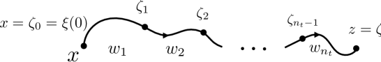
Fig. 1: Concatenations of trajectories to yield a longer time horizon.

In order to test the conjecture that (179) is a suitable generalization of the longer horizon fundamental solution, recall that $W^{\mu,\infty}(\tau,\cdot,\cdot)$ takes the form of the quadratic functional given by (145), see Theorem 12. Combining (145) and (179),

$$W^{\mu,\infty}(t,x,z) =\operatorname*{stat}_{\zeta\in({{\mathscr{X}}}_{\frac{1}{2}})^{n_{t}-1}}\Theta^{\mu}(\tau,x,\zeta,z)\,,\qquad\Theta^{\mu}(\tau,x,\zeta,z)\doteq{{\textstyle{\frac{1}{2}}}}\left\langle\left(\begin{array}[]{c}x\\ \zeta\\ z\end{array}\right),\,\Pi^{\mu}(\tau)\left(\begin{array}[]{c}x\\ \zeta\\ z\end{array}\right)\right\rangle_{\star}$$ (186)

where $\langle\cdot,\,\cdot\rangle_{\star}$ denotes an inner product on $({{\mathscr{X}}}_{\frac{1}{2}})^{n_{t}+1}$, defined for all $\hat{\zeta},\,\hat{\xi}\in({{\mathscr{X}}}_{\frac{1}{2}})^{n_{t}+1}$ by $\langle\hat{\zeta},\hat{\xi}\rangle_{\star}\doteq\sum_{i=1}^{n_{t}+1}\langle\hat{\zeta}_{i},\,\hat{\xi}_{i}\rangle_{\frac{1}{2}}$, and $\Pi^{\mu}(\tau)\in({\mathcal{L}}({{\mathscr{X}}}_{\frac{1}{2}}))^{(n_{t}+1)\times(n_{t}+1)}$ is a matrix of Riesz-spectral operators defined by

$$\Pi^{\mu}(\tau) \doteq\left(\begin{array}[]{c|cccc|c}{\breve{{\mathcal{P}}}}^{\mu,\infty}(\tau)&{\breve{{\mathcal{Q}}}}^{\mu,\infty}(\tau)&0&\cdots&0&0\\ \hline\cr{\breve{{\mathcal{Q}}}}^{\mu,\infty}(\tau)^{\prime}&{\breve{{\mathcal{P}}}}^{\mu,\infty}(\tau)+{\breve{{\mathcal{R}}}}^{\mu,\infty}(\tau)&{\breve{{\mathcal{Q}}}}^{\mu,\infty}(\tau)&\cdots&0&0\\ 0&{\breve{{\mathcal{Q}}}}^{\mu,\infty}(\tau)^{\prime}&{\breve{{\mathcal{P}}}}^{\mu,\infty}(\tau)+{\breve{{\mathcal{R}}}}^{\mu,\infty}(\tau)&\cdots&0&0\\ 0&0&{\breve{{\mathcal{Q}}}}^{\mu,\infty}(\tau)^{\prime}&\cdots&0&0\\ \vdots&\vdots&\vdots&\ddots&\vdots&\vdots\\ 0&0&0&\cdots&{\breve{{\mathcal{Q}}}}^{\mu,\infty}(\tau)&0\\ 0&0&0&\cdots&{\breve{{\mathcal{P}}}}^{\mu,\infty}(\tau)+{\breve{{\mathcal{R}}}}^{\mu,\infty}(\tau)&{\breve{{\mathcal{Q}}}}^{\mu,\infty}(\tau)\\ \hline\cr 0&0&0&\cdots&{\breve{{\mathcal{Q}}}}^{\mu,\infty}(\tau)^{\prime}&{\breve{{\mathcal{R}}}}^{\mu,\infty}(\tau)\end{array}\right)$$ (195)

$$\equiv\left(\begin{array}[]{c|c|c}{\breve{{\mathcal{P}}}}^{\mu,\infty}(\tau)&\Pi_{1,2}^{\mu}(\tau)&0\\ \hline\cr{\Pi}_{1,2}^{\mu}(\tau)^{\prime}&\Pi_{2,2}^{\mu}(\tau)&\Pi_{2,3}^{\mu}(\tau)\\ \hline\cr 0&\Pi_{2,3}^{\mu}(\tau)^{\prime}&{\breve{{\mathcal{R}}}}^{\mu,\infty}(\tau)\end{array}\right)\,.$$ (199)

The existence of a solution of a TPBVP such as (6) on the long horizon $t\in{\mathbb{R}}_{>0}$ requires (by the action principle) that the $\operatorname*{stat}$ in the definition (186) of $W^{\mu,\infty}(t,x,z)$ exist. Define $\zeta^{*}\in({{\mathscr{X}}}_{\frac{1}{2}})^{n_{t}-1}$ by

$$\zeta^{\mu,*}\doteq\operatorname*{arg\,stat}_{\zeta\in({{\mathscr{X}}}_{\frac{1}{2}})^{n_{t}-1}}\Theta^{\mu}(t,x,\zeta,z)\,,$$

and note that $0=\nabla_{\zeta}\Theta^{\mu}(t,x,\zeta^{\mu,*},z)$, where $\nabla_{\zeta}\Theta^{\mu}(t,x,\zeta,z)\in({{\mathscr{X}}}_{\frac{1}{2}})^{n_{t}-1}$ is the Fréchet derivative of $\Theta^{\mu}(t,x,\cdot,z)$ at $\zeta\in({{\mathscr{X}}}_{\frac{1}{2}})^{n_{t}-1}$. Applying (199) yields

$$\Pi_{2,2}^{\mu}(\tau)\,\zeta^{\mu,*} =-\Pi_{1,2}^{\mu}(\tau)^{\prime}\,x-\Pi_{2,3}^{\mu}(\tau)\,z\,.$$ (200)

Hence, on the longer horizon $t\in[\bar{t}^{\mu},2\,\bar{t}^{\mu})$ (for example), the fundamental solution (73) generalizes as per (179) to $W^{\mu,\infty}(t,x,\zeta^{\mu,*})+W^{\mu,\infty}(t,\zeta^{\mu,*},z)$, where $\zeta^{\mu,*}$ solves (200) for $n_{t}\doteq 2$, $\tau\doteq t/2$. This approach generalizes to any fixed longer horizon $t\in{\mathbb{R}}_{>0}$, and taking $\mu\rightarrow 0$ corresponds to sending $n_{t}\rightarrow\infty$ in (179). Furthermore, in this limit, it may be shown that evaluating (179) via (186) and (200) yields the same explicit quadratic representation for the fundamental solution $W^{\mu,\infty}(t,x,z)$, but with $\mu=0$, as presented in Theorem 12.

5 Example

For sufficiently short time horizons, as considered in Section 4.1, the action principle corresponding to the wave equation (1) may be approximated by the optimal control problem (29). This approximation may be extended to longer horizons via the concatenation approach outlined in Section 4.2, and becomes exact in the limit of the perturbation parameter $\mu\in{\mathbb{R}}$ tending to zero (see Theorem 15). Consequently, as the action principle describes all possible solutions to the wave equation (1), including those constrained by any specific combination of boundary data, TPBVPs involving this wave equation may be solved via the optimal control problem (29). The initial velocity $w^{*}(0)$ that solves such a TPBVP may be found via the recipe enumerated in Section 4.1, with $\mu=0$. In particular, step ❹ of that recipe yields the initial velocity that solves a TPBVP as

$$v=w^{*}(0) ={\textstyle{\frac{1}{m}}}\,{{\mathcal{A}}^{\frac{1}{2}}}\,{\mathcal{I}}_{0}\,{{\mathcal{A}}^{\frac{1}{2}}}\,{\nabla}_{x}W^{0,\infty}(t,x,z)={\textstyle{\frac{1}{m}}}\,{\mathcal{A}}\,\left[{\breve{{\mathcal{P}}}}^{0,\infty}(t)\,x+{\breve{{\mathcal{Q}}}}^{0,\infty}(t)\,z^{*}\right]$$

$$={\textstyle{\frac{1}{m}}}\sum_{n=1}^{\infty}\lambda_{n}^{0}\left[p_{n}^{0,\infty}(t)\,\langle x,\,\tilde{\varphi}_{n}\rangle_{\frac{1}{2}}+q_{n}^{0,\infty}(t)\,\langle z^{*},\,\tilde{\varphi}_{n}\rangle_{\frac{1}{2}}\right]\tilde{\varphi}_{n}\,,$$ (201)

where $p_{n}^{0,\infty}$, $q_{n}^{0,\infty}$ are as per (149) and $z^{*}$ is as per (151), after sending $\mu\rightarrow 0$.

(a) Terminal displacement $z(\lambda)$ vs $\lambda$.

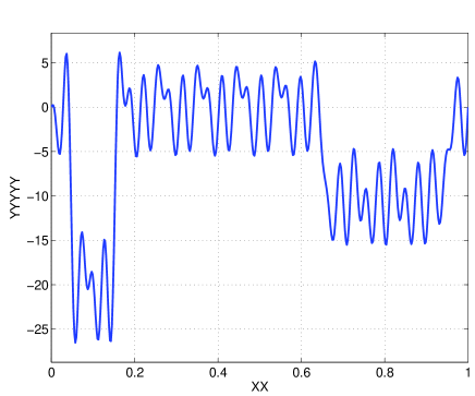
(b) Initial velocity $v(\lambda)$ vs $\lambda$.

Fig. 2: Initial velocity required to achieve terminal displacement.

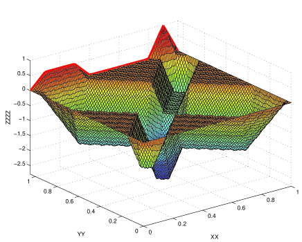
(a) Wave equation solution $u(s,\lambda)$, $s\in{[0,t]}$, $\lambda\in{[0,L]}$.

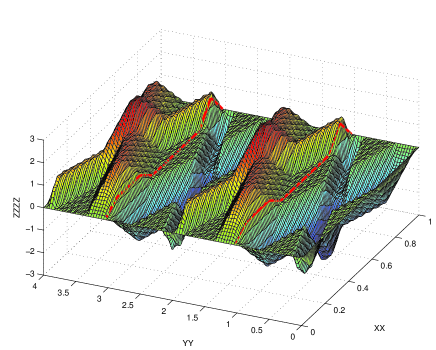
(b) Wave equation solution $u(s,\lambda)$, $s\in{[0,4L({\textstyle{\frac{m}{\kappa}}})^{\frac{1}{2}}]}$, $\lambda\in{[0,L]}$.

Fig. 3: Solutions of wave equation (1).

With $m=\kappa=L=1$ (with appropriate dimensions) in (1), suppose that the specific problem ${\textsf{TPBVP}}(t,x,z)$ is to be solved given the (arbitrary) initial displacement $x=0\in{{\mathscr{X}}}_{0}$, terminal displacement $z\in{{\mathscr{X}}}_{0}$ as per Figure 3(a), and horizon $t\doteq{\textstyle{\frac{\pi\,L}{3}}}\,(\frac{m}{\kappa})^{\frac{1}{2}}$ ($\approx 1.05$). Recall in that case that the terminal payoff $\psi\doteq\psi^{\mu,\infty}(\cdot,z)$ encapsulates the required terminal displacement, and $z^{*}=z$ is required in (201), as per discussion following (151). Applying (201) then yields the required initial velocity illustrated in Figure 3(b) that solves TPBVP (6) via the fundamental solution (73). This solution may be tested by propagating the initial displacement and velocity obtained forward to time $t$ by solving the wave equation (1) directly. (Here, the $C_{0}$-semigroup ${\mathcal{T}}^{\oplus}(\cdot)$ of (54) generated by ${\mathcal{A}}^{\oplus}$ is applied to this end, see for example [3].) The resulting wave equation dynamics are illustrated in Figure 3(a), with the desired terminal displacement clearly achieved. Integration over a longer time period reveals (expected) periodic behaviour, see Figure 3(b).

6 Conclusion

A new fundamental solution based approach to solving a two point boundary value problem for a wave equation is considered. A value functional based characterization of this fundamental solution is formulated via the analysis of an optimal control problem that encapsulates the principle of stationary action. This value functional is shown to enjoy an explicit Riesz-spectral operator based representation via an associated infinite dimensional Hamilton Jacobi Bellman partial differential equation. Application of the fundamental solution obtained is illustrated via a simple example.

Appendix A Properties of operators ${\mathcal{A}}$ and ${{\mathcal{A}}^{\frac{1}{2}}}$

Operators ${\mathcal{A}}$ and ${{\mathcal{A}}^{\frac{1}{2}}}$ are key to the application of the principle of stationary action to obtain the wave dynamics (1) via optimal control. The relevant properties of these operators are largely well-known [3], and are stated without proof unless otherwise indicated.

Lemma 16.

The following properties hold on ${{\mathscr{X}}}$:

1. Operator ${\mathcal{A}}$ is self-adjoint, positive, boundedly invertible, and closed, with

   $${\mathcal{A}}^{\prime}\,x={\mathcal{A}}\,x\,, \forall\,x\in{\textsf{dom\,}}({\mathcal{A}}^{\prime})={\textsf{dom\,}}({\mathcal{A}})={{\mathscr{X}}}_{0}\,,$$

   $${\textsf{ran\,}}({\mathcal{A}})={\textsf{ran\,}}({\mathcal{A}}^{\prime})={{\mathscr{X}}}\,,$$ (202)

   $$\langle x,\,{\mathcal{A}}\,x\rangle=\|\partial x\|^{2}>0\,, \forall\ x\in{\textsf{dom\,}}({\mathcal{A}})={{\mathscr{X}}}_{0}\,,\,x\neq 0\,,$$ (203)

   $${\mathcal{A}}^{-1}\,x=\int_{\Lambda}\hat{A}(\cdot,\zeta)\,x(\zeta)\,d\zeta\,, \hat{A}(\lambda,\zeta)\doteq{\textstyle{\frac{1}{L}}}\left\{\begin{array}[]{cl}(L-\zeta)\,\lambda\,,&0\leq\lambda\leq\zeta\leq L\,,\\ (L-\lambda)\,\zeta\,,&0\leq\zeta<\lambda\leq L\,,\end{array}\right.$$ (206)

   $$\forall\ x\in{\textsf{dom\,}}({\mathcal{A}}^{-1})={{\mathscr{X}}}\,,$$

   $${\textsf{ran\,}}({\mathcal{A}}^{-1})={\textsf{dom\,}}({\mathcal{A}})={{\mathscr{X}}}_{0}\,.$$ (207)

2. Operator ${\mathcal{A}}$ has a unique, positive, self-adjoint, boundedly invertible, and closed square root ${{\mathcal{A}}^{\frac{1}{2}}}$, with

   $${{\mathcal{A}}^{\frac{1}{2}}}\,x\in{\textsf{dom\,}}({{\mathcal{A}}^{\frac{1}{2}}})={{\mathscr{X}}}_{\frac{1}{2}} \forall\ x\in{\textsf{dom\,}}({\mathcal{A}})={{\mathscr{X}}}_{0}\,,$$ (208)

   $${{\mathcal{A}}^{\frac{1}{2}}}\,{{\mathcal{A}}^{\frac{1}{2}}}\,x={\mathcal{A}}\,x\,, \forall\ x\in{\textsf{dom\,}}({\mathcal{A}})={{\mathscr{X}}}_{0}\,,$$ (209)

   $$\|{{\mathcal{A}}^{\frac{1}{2}}}\,x\|=\|\partial x\|=\|x\|_{\frac{1}{2}} \forall\ x\in{\textsf{dom\,}}({\mathcal{A}})={{\mathscr{X}}}_{0}\,,$$ (210)

   $${\mathcal{J}}\,x\doteq\left({{\mathcal{A}}^{\frac{1}{2}}}\right)^{-1}\,x=\left({\mathcal{A}}^{-1}\right)^{\frac{1}{2}}\,x\,, \forall\,x\in{\textsf{dom\,}}({\mathcal{J}})={{\mathscr{X}}}\,,$$

   $${\textsf{ran\,}}({\mathcal{J}})={\textsf{dom\,}}({{\mathcal{A}}^{\frac{1}{2}}})={{\mathscr{X}}}_{\frac{1}{2}}\,,$$ (211)

   $$\left\|{\mathcal{J}}\,x\right\|_{\frac{1}{2}}=\|x\|\,, \forall\,x\in{\textsf{dom\,}}({\mathcal{J}})={{\mathscr{X}}}\,.$$ (212)

Lemma 17.

Operator ${\mathcal{A}}$ of (13) has countably infinite simple eigenvalues given by $\{\lambda_{n}\}_{n=1}^{\infty}$, where eigenvalue $\lambda_{n}$ corresponds to eigenvector $\varphi_{n}\in{\mathcal{B}}$ of (17) (or equivalently $\tilde{\varphi}_{n}\in{\tilde{{\mathcal{B}}}}$) and

$$\lambda_{n}\doteq({\textstyle{\frac{n\,\pi}{L}}})^{2}\,.$$ (213)

Similarly, the square root ${{\mathcal{A}}^{\frac{1}{2}}}$ of operator ${\mathcal{A}}$ has countably infinite simple eigenvalues given by $\{\sqrt{\lambda_{n}}\}_{n=1}^{\infty}$, where eigenvalue $\sqrt{\lambda_{n}}$ corresponds to eigenvector $\varphi_{n}\in{\mathcal{B}}$ (or equivalently in $\tilde{\varphi}_{n}\in{\tilde{{\mathcal{B}}}}$) and $\lambda_{n}$ is as per (213).

Lemma 18.

${\mathcal{B}}$ and ${\tilde{{\mathcal{B}}}}$ of (17) are orthonormal Riesz bases for ${{\mathscr{X}}}$ and ${{\mathscr{X}}}_{\frac{1}{2}}$ respectively.

Lemma 19.

The following properties hold on ${{\mathscr{X}}}$ for any $\mu\in{\mathbb{R}}_{>0}$:

1. Operator ${\mathcal{I}}_{\mu}$ of (106) is bounded, linear, self-adjoint, positive, with

   $${\mathcal{I}}_{\mu}\,x\in{\textsf{dom\,}}({\mathcal{A}})={{\mathscr{X}}}_{0} \forall\ x\in{\textsf{dom\,}}({\mathcal{I}}_{\mu})={{\mathscr{X}}}\,,$$ (214)

   $${\mathcal{I}}_{\mu}\,x=\int_{\Lambda}I_{\mu}(\cdot,\zeta)\,x(\zeta)\,d\zeta\,, I_{\mu}(\lambda,\zeta)\doteq\frac{1}{\mu\,\sinh({\textstyle{\frac{L}{\mu}}})}\left\{\begin{aligned} \sinh({\textstyle{\frac{\lambda}{\mu}}})\,\sinh({\textstyle{\frac{L-\zeta}{\mu}}})\,,&\quad 0\leq\lambda\leq\zeta\leq L\,,\\ \sinh({\textstyle{\frac{\zeta}{\mu}}})\,\sinh({\textstyle{\frac{L-\lambda}{\mu}}})\,,&\quad 0\leq\zeta\leq\lambda\leq L\,,\end{aligned}\right.$$

   $$\forall\ x\in{\textsf{dom\,}}({\mathcal{I}}_{\mu})={{\mathscr{X}}}\,.$$ (215)

2. Operator ${\mathcal{I}}_{\mu}$ has a unique, bounded, linear, self-adjoint, and positive square root ${\mathcal{I}}_{\mu}^{\frac{1}{2}}$, with

   $${\mathcal{I}}_{\mu}^{\frac{1}{2}}\,x\in{\textsf{dom\,}}({{\mathcal{A}}^{\frac{1}{2}}})={{\mathscr{X}}}_{\frac{1}{2}} \forall\ x\in{\textsf{dom\,}}({\mathcal{I}}_{\mu}^{\frac{1}{2}})={{\mathscr{X}}}\,,$$ (216)

   $${\mathcal{I}}_{\mu}^{\frac{1}{2}}\,{\mathcal{I}}_{\mu}^{\frac{1}{2}}\,x={\mathcal{I}}_{\mu}\,x \forall\ x\in{\textsf{dom\,}}({\mathcal{I}}_{\mu}^{\frac{1}{2}})={\textsf{dom\,}}({\mathcal{I}}_{\mu})={{\mathscr{X}}}\,,$$ (217)

3. Operators ${\mathcal{I}}_{\mu}$, ${\mathcal{I}}_{\mu}^{\frac{1}{2}}$, ${\mathcal{A}}$, and ${\mathcal{A}}^{\frac{1}{2}}$ commute, with

   $${\mathcal{I}}_{\mu}^{\frac{1}{2}}\,{\mathcal{A}}^{\frac{1}{2}}\,x={\mathcal{A}}^{\frac{1}{2}}\,{\mathcal{I}}_{\mu}^{\frac{1}{2}}\,x\,,\quad{\mathcal{I}}_{\mu}\,{{\mathcal{A}}^{\frac{1}{2}}}\,x={{\mathcal{A}}^{\frac{1}{2}}}\,{\mathcal{I}}_{\mu}\,x \forall\ x\in{\textsf{dom\,}}({{\mathcal{A}}^{\frac{1}{2}}})={{\mathscr{X}}}_{\frac{1}{2}}\,.$$ (218)

   $${\mathcal{I}}_{\mu}\,{\mathcal{A}}\,x={\mathcal{A}}\,{\mathcal{I}}_{\mu}\,x\,,\quad{\mathcal{I}}_{\mu}^{\frac{1}{2}}\,{\mathcal{A}}\,x={\mathcal{A}}\,{\mathcal{I}}_{\mu}^{\frac{1}{2}}\,x \forall\ x\in{\textsf{dom\,}}({\mathcal{A}})={{\mathscr{X}}}_{0}\,,$$ (219)

4. Selected compositions of operators ${\mathcal{I}}_{\mu}$, ${\mathcal{I}}_{\mu}^{\frac{1}{2}}$, ${\mathcal{A}}$, and ${\mathcal{A}}^{\frac{1}{2}}$ define bounded linear operators, with

   $${\mathcal{A}}\,{\mathcal{I}}_{\mu},\,{{\mathcal{A}}^{\frac{1}{2}}}\,{\mathcal{I}}_{\mu}^{\frac{1}{2}}\in{\mathcal{L}}({{\mathscr{X}}})\,,$$ (220)

   $${\mathcal{A}}\,{\mathcal{I}}_{\mu}\in{\mathcal{L}}({{\mathscr{X}}}_{\frac{1}{2}})\,,$$ (221)

   $${{\mathcal{A}}^{\frac{1}{2}}}\,{\mathcal{I}}_{\mu}^{\frac{1}{2}}\,{{\mathcal{A}}^{\frac{1}{2}}}\in{\mathcal{L}}({{\mathscr{X}}}_{\frac{1}{2}};{{\mathscr{X}}})\,.$$ (222)

Proof.

(i) Fix any $x\in{\textsf{dom\,}}({\mathcal{A}})={{\mathscr{X}}}_{0}$. Consequently, ${\mathcal{A}}\,x\in{{\mathscr{X}}}$, and

$$\langle x,\,({\mathcal{I}}+\mu^{2}\,{\mathcal{A}})\,x\rangle =\|x\|^{2}+\mu^{2}\,\langle x,\,{\mathcal{A}}\,x\rangle\geq\|x\|^{2}\,,$$

where the inequality follows by positivity of ${\mathcal{A}}$, see assertion (203) of Lemma 16. That is, ${\mathcal{I}}+\mu^{2}\,{\mathcal{A}}$ is both positive and coercive [3, Definition A.3.71, p.606]. It is also self-adjoint by (202). Hence, ${\mathcal{I}}+\mu^{2}\,{\mathcal{A}}$ is boundedly invertible, see for example [3, Example A.4.2, p.609] and [13, Problem 10, p.535]. In particular, ${\mathcal{I}}_{\mu}\doteq({\mathcal{I}}+\mu^{2}\,{\mathcal{A}})^{-1}\in{\mathcal{L}}({{\mathscr{X}}})$. In order to show that ${\mathcal{I}}_{\mu}$ is also self-adjoint and positive (but not coercive), fix any $y,\,\eta\in{{\mathscr{X}}}$, and define $x,\,\xi\in{{\mathscr{X}}}_{0}$ by $x\doteq{\mathcal{I}}_{\mu}\,y$ and $\xi={\mathcal{I}}_{\mu}\,\eta$. As ${\mathcal{I}}+\mu^{2}\,{\mathcal{A}}$ is self-adjoint, $\langle y,\,{\mathcal{I}}_{\mu}\,\eta\rangle=\langle({\mathcal{I}}+\mu^{2}\,{\mathcal{A}})\,x,\,\xi\rangle=\langle x,\,({\mathcal{I}}+\mu^{2}\,{\mathcal{A}})\,\xi\rangle=\langle{\mathcal{I}}_{\mu}\,y,\,\eta\rangle$. As $y,\,\eta\in{{\mathscr{X}}}$ are arbitrary, it follows that ${\mathcal{I}}_{\mu}$ is also self-adjoint. Furthermore, with $y=\eta$, $\langle y,\,{\mathcal{I}}_{\mu}\,y\rangle=\langle({\mathcal{I}}+\mu^{2}\,{\mathcal{A}})\,x,\,x\rangle\geq\|x\|^{2}=\|{\mathcal{I}}_{\mu}\,y\|^{2}$. As $I_{\mu}$ is invertible, the right-hand side is zero if and only if $y=0$. Hence, ${\mathcal{I}}_{\mu}$ is positive. However, ${\mathcal{I}}_{\mu}$ is not coercive, as it has eigenvalues arbitrarily close to zero. For example, select $y\doteq\psi_{n}$, with $\psi_{n}$ is as per (17). Note that $\|\psi_{n}\|=1$. Applying Lemma 17, it is straightforward to show that $\langle\psi_{n},\,{\mathcal{I}}_{\mu}\,\psi_{n}\rangle=\frac{1}{1+\mu^{2}\,\lambda_{n}}\,\|\psi_{n}\|^{2}=\frac{1}{1+\mu^{2}\,({\textstyle{\frac{n\,\pi}{L}}})^{2}}\,\|\psi_{n}\|^{2}$ for all $n\in{\mathbb{N}}$. Note in particular that the coefficient on the right-hand side may be made arbitrarily small for sufficiently large $n\in{\mathbb{N}}$. Hence, ${\mathcal{I}}_{\mu}$ cannot be coercive.

It remains to be shown that (214) and (215) hold. Fix any $x\in{{\mathscr{X}}}$. By noting that ${\mathcal{I}}-{\mathcal{I}}_{\mu}\in{\mathcal{L}}({{\mathscr{X}}})$, the definition (106) of ${\mathcal{I}}_{\mu}$ implies that

$$\infty >{\textstyle{\frac{1}{\mu^{2}}}}\,\|({\mathcal{I}}-{\mathcal{I}}_{\mu})\,x\|={\textstyle{\frac{1}{\mu^{2}}}}\,\|([{\mathcal{I}}+\mu^{2}\,{\mathcal{A}}]\,{\mathcal{I}}_{\mu}-{\mathcal{I}}_{\mu})\,x\|=\|{\mathcal{A}}\,{\mathcal{I}}_{\mu}\,x\|\,.$$ (223)

Hence, ${\mathcal{I}}_{\mu}\,x\in{\textsf{dom\,}}({\mathcal{A}})={{\mathscr{X}}}_{0}$ for any $x\in{{\mathscr{X}}}$, so that (214) holds. Given the kernel $I_{\mu}$ as defined in (215), define the operator ${\widehat{{\mathcal{I}}}}_{\mu}$ by

$${\widehat{{\mathcal{I}}}}_{\mu}\,x \doteq\int_{\Lambda}I_{\mu}(\cdot,\zeta)\,x(\zeta)\,d\zeta\,,\quad{\textsf{dom\,}}({\widehat{{\mathcal{I}}}}_{\mu})\doteq{{\mathscr{X}}}\,,$$ (224)

and note that ${\widehat{{\mathcal{I}}}}_{\mu}\in{\mathcal{L}}({{\mathscr{X}}})$ by inspection. Fix any $x\in{{\mathscr{X}}}$ and define $y\doteq{\mathcal{I}}_{\mu}\,x\in{{\mathscr{X}}}_{0}$. Hence, ${\mathcal{A}}\,y\in{{\mathscr{X}}}$, and ${\widehat{{\mathcal{I}}}}_{\mu}\,{\mathcal{A}}\,y=\int_{\Lambda}I_{\mu}(\cdot,\zeta)\,[-\partial^{2}\,y(\zeta)]\,d\zeta=-\int_{\Lambda}[\partial_{2}^{2}I_{\mu}(\cdot,\zeta)]\,y(\zeta)\,d\zeta$, where $\partial_{2}^{2}I_{\mu}(\lambda,\zeta)\doteq{\textstyle{\frac{1}{\mu^{2}}}}\,I_{\mu}(\lambda,\zeta)-{\textstyle{\frac{1}{\mu^{2}}}}\,\delta(\lambda-\zeta)$ is the second weak derivative of $I_{\mu}(\lambda,\cdot)$, $\lambda\in\Lambda$ fixed. Note in particular that the boundary conditions $y(0)=0=y(L)$ have been used here. Consequently, ${\widehat{{\mathcal{I}}}}_{\mu}\,{\mathcal{A}}\,y=-{\textstyle{\frac{1}{\mu^{2}}}}\int_{\Lambda}[I_{\mu}(\cdot,\zeta)-\delta(\cdot-\zeta)]\,y(\zeta)\,d\zeta=-{\textstyle{\frac{1}{\mu^{2}}}}({\widehat{{\mathcal{I}}}}_{\mu}\,y-y)$, so that ${\widehat{{\mathcal{I}}}}_{\mu}\,({\mathcal{I}}+\mu^{2}\,{\mathcal{A}})\,y=y$. Recalling the definition of $y$, it follows immediately that ${\widehat{{\mathcal{I}}}}_{\mu}\,x={\mathcal{I}}_{\mu}\,x$. As $x\in{{\mathscr{X}}}$ is arbitrary, assertion (215) follows.

(ii) The existence of a unique, bounded linear, self-adjoint, and positive square root ${\mathcal{I}}_{\mu}^{\frac{1}{2}}$ follows (for example) by [2, Theorem 4]. (Alternatively, see [3, Lemma A.3.73, p.606].)

(iii) Fix $x\in{{\mathscr{X}}}_{\frac{1}{2}}$. By definition, ${{\mathcal{A}}^{\frac{1}{2}}}\,x\in{{\mathscr{X}}}={\textsf{dom\,}}({\mathcal{I}}_{\mu}^{\frac{1}{2}})$, and

$${\mathcal{I}}_{\mu}\,{{\mathcal{A}}^{\frac{1}{2}}}\,x =({\mathcal{I}}+\mu^{2}\,{\mathcal{A}})^{-1}\,{{\mathcal{A}}^{\frac{1}{2}}}\,x=({\mathcal{J}}\,[{\mathcal{I}}+\mu^{2}\,{\mathcal{A}}])^{-1}\,x=({\mathcal{J}}+\mu^{2}\,{\mathcal{J}}\,{{\mathcal{A}}^{\frac{1}{2}}}\,{{\mathcal{A}}^{\frac{1}{2}}})^{-1}\,x$$

$$=({\mathcal{J}}+\mu^{2}\,{{\mathcal{A}}^{\frac{1}{2}}}\,{{\mathcal{A}}^{\frac{1}{2}}}\,{\mathcal{J}})^{-1}\,x=([{\mathcal{I}}+\mu^{2}\,{\mathcal{A}}]\,{\mathcal{J}})^{-1}\,x={{\mathcal{A}}^{\frac{1}{2}}}\,({\mathcal{I}}+\mu^{2}\,{\mathcal{A}})^{-1}\,x={{\mathcal{A}}^{\frac{1}{2}}}\,{\mathcal{I}}_{\mu}\,x\,,$$

so that right-hand equality in assertion (218) holds. The remaining equalities follow similarly, with $x\in{{\mathscr{X}}}_{0}$ yielding assertion (219).

(iv) The first assertion in (220) follows from the proof of (i) above. In particular, ${\mathcal{I}}-{\mathcal{I}}_{\mu}\in{\mathcal{L}}({{\mathscr{X}}})$ and (223) imply that $\|{\mathcal{A}}\,{\mathcal{I}}_{\mu}\|={\textstyle{\frac{1}{\mu^{2}}}}\,\|{\mathcal{I}}-{\mathcal{I}}_{\mu}\|<\infty$, as required. In order to prove the second assertion of (220), note that for any $x\in{{\mathscr{X}}}_{\frac{1}{2}}$, (219) implies that

$$\|{{\mathcal{A}}^{\frac{1}{2}}}\,{\mathcal{I}}_{\mu}^{\frac{1}{2}}\,x\|^{2} =\langle x,\,{\mathcal{I}}_{\mu}^{\frac{1}{2}}\,{\mathcal{A}}\,{\mathcal{I}}_{\mu}^{\frac{1}{2}}\,x\rangle=\langle x,\,{\mathcal{A}}\,{\mathcal{I}}_{\mu}\,x\rangle\leq\|x\|\,\|{\mathcal{A}}\,{\mathcal{I}}_{\mu}\,x\|\leq\|{\mathcal{A}}\,{\mathcal{I}}_{\mu}\|\|x\|^{2}\,.$$

Hence, the restriction ${\mathcal{R}}_{\mu}$ of ${{\mathcal{A}}^{\frac{1}{2}}}\,{\mathcal{I}}_{\mu}^{\frac{1}{2}}:{{\mathscr{X}}}{\rightarrow}{{\mathscr{X}}}$ to the domain ${{\mathscr{X}}}_{\frac{1}{2}}\subset{{\mathscr{X}}}$ is bounded and linear on that domain. However, as ${\overline{{{\mathscr{X}}}_{\frac{1}{2}}}}={{\mathscr{X}}}$, ${\mathcal{R}}_{\mu}$ can be uniquely extended to an operator ${\mathcal{E}}_{\mu}\in{\mathcal{L}}({{\mathscr{X}}})$ (see for example [13, Theorem 2.7-11, p.100]) that satisfies ${\mathcal{E}}_{\mu}\,x={\mathcal{R}}_{\mu}\,x={{\mathcal{A}}^{\frac{1}{2}}}\,{\mathcal{I}}_{\mu}^{\frac{1}{2}}\,x$ for all $x\in{{\mathscr{X}}}_{\frac{1}{2}}$. Fix $y\in{{\mathscr{X}}}$. Hence, for any $x\in{{\mathscr{X}}}_{\frac{1}{2}}$, $\|{\mathcal{E}}_{\mu}\,y-{{\mathcal{A}}^{\frac{1}{2}}}\,{\mathcal{I}}_{\mu}^{\frac{1}{2}}\,y\|\leq\|{\mathcal{E}}_{\mu}\,x-{{\mathcal{A}}^{\frac{1}{2}}}\,{\mathcal{I}}_{\mu}^{\frac{1}{2}}\,x\|+\|({\mathcal{E}}_{\mu}-{{\mathcal{A}}^{\frac{1}{2}}}\,{\mathcal{I}}_{\mu}^{\frac{1}{2}})\,(y-x)\|\leq\|{\mathcal{E}}_{\mu}-{{\mathcal{A}}^{\frac{1}{2}}}\,{\mathcal{I}}_{\mu}^{\frac{1}{2}}\|\,\|y-x\|$. Consequently, as $x\in{{\mathscr{X}}}_{\frac{1}{2}}$ is arbitrary and ${\overline{{{\mathscr{X}}}_{\frac{1}{2}}}}={{\mathscr{X}}}$, implies that $\|{\mathcal{E}}_{\mu}\,y-{{\mathcal{A}}^{\frac{1}{2}}}\,{\mathcal{I}}_{\mu}^{\frac{1}{2}}\,y\|\leq\|{\mathcal{E}}_{\mu}-{{\mathcal{A}}^{\frac{1}{2}}}\,{\mathcal{I}}_{\mu}^{\frac{1}{2}}\|\,\inf_{x\in{{\mathscr{X}}}_{\frac{1}{2}}}\|y-x\|=0$. As $y\in{{\mathscr{X}}}$ is arbitrary, ${\mathcal{E}}_{\mu}\equiv{{\mathcal{A}}^{\frac{1}{2}}}{\mathcal{I}}_{\mu}^{\frac{1}{2}}$. Recalling that ${\mathcal{E}}_{\mu}\in{\mathcal{L}}({{\mathscr{X}}})$ completes the proof of assertion (220).

In order to prove assertion (221), note that ${{\mathcal{A}}^{\frac{1}{2}}}$ and ${\mathcal{I}}_{\mu}$ commute on ${{\mathscr{X}}}_{\frac{1}{2}}$ by (218). Hence, with $x\in{{\mathscr{X}}}_{\frac{1}{2}}$. $\|{\mathcal{A}}\,{\mathcal{I}}_{\mu}\,x\|_{\frac{1}{2}}=\|{{\mathcal{A}}^{\frac{1}{2}}}\,{\mathcal{I}}_{\mu}\,{{\mathcal{A}}^{\frac{1}{2}}}\,x\|_{\frac{1}{2}}=\|{\mathcal{A}}\,{\mathcal{I}}_{\mu}\,({{\mathcal{A}}^{\frac{1}{2}}}\,x)\|\leq\|{\mathcal{A}}\,{\mathcal{I}}_{\mu}\|\,\|{{\mathcal{A}}^{\frac{1}{2}}}\,x\|=\|{\mathcal{A}}\,{\mathcal{I}}_{\mu}\|\,\|x\|_{\frac{1}{2}}$. As ${\mathcal{A}}\,{\mathcal{I}}_{\mu}\in{\mathcal{L}}({{\mathscr{X}}})$ by (220), assertion (221) immediately follows.

Finally, in order to prove assertion (222), note that (220) implies that $\|{{\mathcal{A}}^{\frac{1}{2}}}\,{\mathcal{I}}_{\mu}^{\frac{1}{2}}\,{{\mathcal{A}}^{\frac{1}{2}}}\,x\|\leq\|{{\mathcal{A}}^{\frac{1}{2}}}\,{\mathcal{I}}_{\mu}^{\frac{1}{2}}\|\,\|{{\mathcal{A}}^{\frac{1}{2}}}\,x\|=\|{{\mathcal{A}}^{\frac{1}{2}}}\,{\mathcal{I}}_{\mu}^{\frac{1}{2}}\|\,\|x\|_{\frac{1}{2}}$ for any $x\in{{\mathscr{X}}}_{\frac{1}{2}}$. Consequently, $\sup_{x\in{{\mathscr{X}}}_{\frac{1}{2}},\|x\|_{\frac{1}{2}}\neq 0}\frac{\|{{\mathcal{A}}^{\frac{1}{2}}}\,{\mathcal{I}}_{\mu}^{\frac{1}{2}}\,{{\mathcal{A}}^{\frac{1}{2}}}\,x\|}{\|x\|_{\frac{1}{2}}}\leq\|{{\mathcal{A}}^{\frac{1}{2}}}\,{\mathcal{I}}_{\mu}^{\frac{1}{2}}\|<\infty$ as required. ∎

Appendix B Riesz-spectral operators

It is useful to consider self-adjoint operators of the form

$${\breve{{\mathcal{F}}}}\,x \doteq\sum_{n=1}^{\infty}f_{n}\,\langle x,\,\tilde{\varphi}_{n}\rangle_{\frac{1}{2}}\,\tilde{\varphi}_{n}\,,\quad{\textsf{dom\,}}({\breve{{\mathcal{F}}}})\doteq\left\{x\in{{\mathscr{X}}}_{\frac{1}{2}}\,\biggl{|}\,{\breve{{\mathcal{F}}}}\,x\in{{\mathscr{X}}}_{\frac{1}{2}}\right\},$$ (225)

where the set $\{f_{n}\}_{n\in{\mathbb{N}}}\subset{\mathbb{R}}$ of eigenvalues of ${\breve{{\mathcal{F}}}}$ is simple and has a totally disconnected closure (i.e. no two elements of this closure can be joined by a segment lying entirely within it), and ${\tilde{{\mathcal{B}}}}=\{\tilde{\varphi}_{n}\}_{n\in{\mathbb{N}}}$ (enumerating the corresponding eigenvectors of ${\breve{{\mathcal{F}}}}$) is the orthonormal Riesz basis defined by (17). This type of operator is closed and densely defined on ${{\mathscr{X}}}_{\frac{1}{2}}$, see [3, Example 2.1.13, p.29], and is referred to as a Riesz-spectral operator on ${{\mathscr{X}}}_{\frac{1}{2}}$, see [3, Definition 2.3.4, p.41]. Operators ${\mathcal{A}}$ and ${{\mathcal{A}}^{\frac{1}{2}}}$ are Riesz-spectral operators, and may be similarly represented, see [3, Theorem 2.3.5] and Lemma 25 below. The identity ${\mathcal{I}}$ also takes the form (225), with

$$x={\mathcal{I}}\,x \doteq\sum_{n=1}^{\infty}\langle x,\,\tilde{\varphi}_{n}\rangle_{\frac{1}{2}}\,\tilde{\varphi}_{n}\,,\quad{\textsf{dom\,}}({\mathcal{I}})\equiv{{\mathscr{X}}}_{\frac{1}{2}}\,.$$ (226)

However, ${\mathcal{I}}$ is not a Riesz-spectral operator (its eigenvalues are repeated at $1$, and so are not simple). Nevertheless, $\|x\|_{\frac{1}{2}}^{2}=\sum_{n=1}^{\infty}|\langle x,\,\tilde{\varphi}_{n}\rangle_{\frac{1}{2}}|^{2}$ for all $x\in{{\mathscr{X}}}_{\frac{1}{2}}$, see [3, Corollary 2.3.3, p.40].

The remainder of this appendix documents some useful properties of Riesz-spectral operators that are applied in the main body of the paper. Unless otherwise indicated, proofs of these properties are considered standard and are omitted.

Lemma 20.

The domain ${\textsf{dom\,}}({\breve{{\mathcal{F}}}})$ of a Riesz-spectral operator ${\breve{{\mathcal{F}}}}$ of the form (225) is equivalently given by

$${\textsf{dom\,}}({\breve{{\mathcal{F}}}}) =\left\{x\in{{\mathscr{X}}}_{\frac{1}{2}}\,\left|\,\|{\breve{{\mathcal{F}}}}\,x\|_{\frac{1}{2}}<\infty\right.\right\}\,,\qquad\|{\breve{{\mathcal{F}}}}\,x\|_{\frac{1}{2}}^{2}=\sum_{n=1}^{\infty}|f_{n}|^{2}\,|\langle x,\,\tilde{\varphi}_{n}\rangle_{\frac{1}{2}}|^{2}\,.$$ (227)

Lemma 21.

Let ${\breve{{\mathcal{F}}}}$ and ${\breve{{\mathcal{G}}}}$ denote two Riesz-spectral operators of the form (225), with respective point spectra $\sigma_{p}({\breve{{\mathcal{F}}}})=\{f_{n}\}_{n=1}^{\infty}$ and $\sigma_{p}({\breve{{\mathcal{G}}}})=\{g_{n}\}_{n=1}^{\infty}$, and domains ${\textsf{dom\,}}({\breve{{\mathcal{F}}}})$, ${\textsf{dom\,}}({\breve{{\mathcal{G}}}})$ as per (227). Suppose additionally that $\{f_{n}\,g_{n}\}_{n=1}^{\infty}$ is simple, and its closure is totally disconnected. Then, the composition ${\breve{{\mathcal{F}}}}\,{\breve{{\mathcal{G}}}}$ is also a Riesz-spectral operator of the form (225), with

$${\breve{{\mathcal{F}}}}\,{\breve{{\mathcal{G}}}}\,x =\sum_{n=1}^{\infty}f_{n}\,g_{n}\,\langle x,\,\tilde{\varphi}_{n}\rangle_{\frac{1}{2}}\,\tilde{\varphi}_{n}\,,\quad{\textsf{dom\,}}({\breve{{\mathcal{F}}}}\,{\breve{{\mathcal{G}}}})=\left\{x\in{\textsf{dom\,}}({\breve{{\mathcal{G}}}})\subset{{\mathscr{X}}}_{\frac{1}{2}}\,\biggl{|}\,{\breve{{\mathcal{G}}}}\,x\in{\textsf{dom\,}}({\breve{{\mathcal{F}}}})\right\}.$$ (228)

Corollary 22.

Let ${\breve{{\mathcal{F}}}}$ and ${\breve{{\mathcal{G}}}}$ be Riesz-spectral operators as per Lemma 21. Then, the domain of the composition ${\breve{{\mathcal{F}}}}\,{\breve{{\mathcal{G}}}}$ of (228) is equivalently given by

$${\textsf{dom\,}}({\breve{{\mathcal{F}}}}\,{\breve{{\mathcal{G}}}}) =\left\{x\in{{\mathscr{X}}}_{\frac{1}{2}}\,\left|\,\sum_{n=1}^{\infty}(1+|f_{n}|^{2})\,|g_{n}|^{2}\,|\langle x,\,\tilde{\varphi}_{n}\rangle_{\frac{1}{2}}|^{2}<\infty\right.\right\}.$$ (229)

If additionally there exists $f_{-}\in{\mathbb{R}}_{>0}$ such that $|f_{n}|\geq f_{-}$ for all $n\in{\mathbb{N}}$, then the domain ${\textsf{dom\,}}({\breve{{\mathcal{F}}}}\,{\breve{{\mathcal{G}}}})$ specified via (225) or (229) is equivalently given by

$${\textsf{dom\,}}({\breve{{\mathcal{F}}}}\,{\breve{{\mathcal{G}}}}) =\left\{x\in{{\mathscr{X}}}_{\frac{1}{2}}\,\left|\,\sum_{n=1}^{\infty}|f_{n}\,g_{n}|^{2}\,|\langle x,\,\tilde{\varphi}_{n}\rangle_{\frac{1}{2}}|^{2}<\infty\right.\right\}.$$ (230)

Proof.

Recalling (228), $x\in{\textsf{dom\,}}({\breve{{\mathcal{F}}}}\,{\breve{{\mathcal{G}}}})$ if and only if $x\in{\textsf{dom\,}}({\breve{{\mathcal{G}}}})$ and ${\breve{{\mathcal{G}}}}\,x\in{\textsf{dom\,}}({\breve{{\mathcal{F}}}})$. These respective properties hold if and only if

$$\infty >\sum_{n=1}^{\infty}|g_{n}|^{2}\,|\langle x,\,\tilde{\varphi}_{n}\rangle_{\frac{1}{2}}|^{2}\,,\quad\infty>\sum_{n=1}^{\infty}|f_{n}|^{2}\,|\langle{\breve{{\mathcal{G}}}}\,x,\,\tilde{\varphi}_{n}\rangle_{\frac{1}{2}}|^{2}=\sum_{n=1}^{\infty}|f_{n}\,g_{n}|^{2}\,|\langle x,\,\tilde{\varphi}_{n}\rangle_{\frac{1}{2}}|^{2}\,.$$ (231)

So, the domain of ${\breve{{\mathcal{F}}}}\,{\breve{{\mathcal{G}}}}$ is given by

$${\textsf{dom\,}}({\breve{{\mathcal{F}}}}\,{\breve{{\mathcal{G}}}}) =\left\{x\in{\textsf{dom\,}}({\breve{{\mathcal{G}}}})\subset{{\mathscr{X}}}_{\frac{1}{2}}\,\biggl{|}\,{\breve{{\mathcal{G}}}}\,x\in{\textsf{dom\,}}({\breve{{\mathcal{F}}}})\right\}=\left\{x\in{\textsf{dom\,}}({\breve{{\mathcal{G}}}})\subset{{\mathscr{X}}}_{\frac{1}{2}}\,\left|\,\sum_{n=1}^{\infty}|f_{n}\,g_{n}|^{2}\,|\langle x,\,\tilde{\varphi}_{n}\rangle_{\frac{1}{2}}|^{2}<\infty\right.\right\}$$

$$=\left\{x\in{{\mathscr{X}}}_{\frac{1}{2}}\,\left|\,\sum_{n=1}^{\infty}(1+|f_{n}|^{2})\,|g_{n}|^{2}\,|\langle x,\,\tilde{\varphi}_{n}\rangle_{\frac{1}{2}}|^{2}<\infty\right.\right\},$$

as specified by (229). Suppose additionally that there exists $f_{-}\in{\mathbb{R}}_{>0}$ such that $|f_{n}|\geq f_{-}$ for all $n\in{\mathbb{N}}$. Define the domain candidate ${\mathscr{D}}$ as per (230), that is ${\mathscr{D}}\doteq\left\{x\in{{\mathscr{X}}}_{\frac{1}{2}}\,\left|\,\sum_{n=1}^{\infty}|f_{n}\,g_{n}|^{2}\,|\langle x,\,\tilde{\varphi}_{n}\rangle_{\frac{1}{2}}|^{2}<\infty\right.\right\}$. Fix any $x\in{\textsf{dom\,}}({\breve{{\mathcal{F}}}}\,{\breve{{\mathcal{G}}}})$ via (229). By inspection, it immediately follows that $x\in{\mathscr{D}}$. That is, ${\textsf{dom\,}}({\breve{{\mathcal{F}}}}\,{\breve{{\mathcal{G}}}})\subset{\mathscr{D}}$. In order to prove the opposite direction, fix any $x\in{\mathscr{D}}$, and note that the second inequality in (231) implies the first. In particular,

$$\infty >\sum_{n=1}^{\infty}|f_{n}\,g_{n}|^{2}\,|\langle x,\,\tilde{\varphi}_{n}\rangle_{\frac{1}{2}}|^{2}>f_{-}^{2}\,\sum_{n=1}^{\infty}|g_{n}|^{2}\,|\langle x,\,\tilde{\varphi}_{n}\rangle_{\frac{1}{2}}|^{2}\quad\stackrel{{\scriptstyle f_{-}\in{\mathbb{R}}_{>0}}}{{\Longrightarrow}}\quad\infty>\sum_{n=1}^{\infty}|g_{n}|^{2}\,|\langle x,\,\tilde{\varphi}_{n}\rangle_{\frac{1}{2}}|^{2}\,,$$ (232)

which implies that $\infty>\sum_{n=1}^{\infty}|f_{n}\,g_{n}|^{2}\,|\langle x,\,\tilde{\varphi}_{n}\rangle_{\frac{1}{2}}|^{2}+\sum_{n=1}^{\infty}|g_{n}|^{2}\,|\langle x,\,\tilde{\varphi}_{n}\rangle_{\frac{1}{2}}|^{2}=\sum_{n=1}^{\infty}(1+|f_{n}|^{2})\,|g_{n}|^{2}\,|\langle x,\,\tilde{\varphi}_{n}\rangle_{\frac{1}{2}}|^{2}$. Consequently, $x\in{\mathscr{D}}$ implies that $x\in{\textsf{dom\,}}({\breve{{\mathcal{F}}}}\,{\breve{{\mathcal{G}}}})$, or ${\mathscr{D}}\subset{\textsf{dom\,}}({\breve{{\mathcal{F}}}}\,{\breve{{\mathcal{G}}}})$. Combining this with the earlier conclusion that ${\mathscr{D}}\supset{\textsf{dom\,}}({\breve{{\mathcal{F}}}}\,{\breve{{\mathcal{G}}}})$ yields that ${\mathscr{D}}\equiv{\textsf{dom\,}}({\breve{{\mathcal{F}}}}\,{\breve{{\mathcal{G}}}})$. That is, (230) holds as required. ∎

Lemma 23.

Let ${\breve{{\mathcal{F}}}}$, ${\breve{{\mathcal{F}}}}^{\sharp}$ denote a pair of Riesz-spectral operators of the form (225), with point spectra $0\not\in\sigma_{p}({\breve{{\mathcal{F}}}})=\{f_{n}\}_{n=1}^{\infty}$ and $\sigma_{p}({\breve{{\mathcal{F}}}}^{\sharp})=\{{\textstyle{\frac{1}{f_{n}}}}\}_{n=1}^{\infty}$. Then,

$${\breve{{\mathcal{F}}}}\,{\breve{{\mathcal{F}}}}^{\sharp}\,x =x\,,\quad\forall\ x\in{\textsf{dom\,}}({\breve{{\mathcal{F}}}}^{\sharp})\,, {\breve{{\mathcal{F}}}}^{\sharp}\,{\breve{{\mathcal{F}}}}\,x =x\,,\quad\forall\ x\in{\textsf{dom\,}}({\breve{{\mathcal{F}}}})\,.$$ (233)

Corollary 24.

A Riesz operator ${\breve{{\mathcal{F}}}}$ on ${{\mathscr{X}}}_{\frac{1}{2}}$ with point spectrum satisfying $0\notin\sigma_{p}({\breve{{\mathcal{F}}}})=\{f_{n}\}_{n=1}^{\infty}$ is invertible. Furthermore, its inverse ${\breve{{\mathcal{F}}}}^{-1}$ is also a Riesz-spectral operator on ${{\mathscr{X}}}_{\frac{1}{2}}$, and is given by

$${\breve{{\mathcal{F}}}}^{-1}\,x =\sum_{n=1}^{\infty}{\textstyle{\frac{1}{f_{n}}}}\,\langle x,\,\tilde{\varphi}_{n}\rangle_{\frac{1}{2}}\tilde{\varphi}_{n}\,,\quad{\textsf{dom\,}}({\breve{{\mathcal{F}}}}^{-1})=\left\{x\in{{\mathscr{X}}}_{\frac{1}{2}}\,\biggl{|}\,\sum_{n=1}^{\infty}|{\textstyle{\frac{1}{f_{n}}}}|^{2}\,|\langle x,\,\tilde{\varphi}_{n}\rangle_{\frac{1}{2}}|^{2}<\infty\right\}.$$ (234)

It is well known by Riesz’s Lemma that the identity ${\mathcal{I}}$ of (226) is not a Riesz-spectral operator on ${{\mathscr{X}}}_{\frac{1}{2}}$. Consequently, the composition of a Riesz-spectral operator ${\breve{{\mathcal{F}}}}$ and its inverse ${\breve{{\mathcal{F}}}}^{-1}$ (also a Riesz-spectral operator, by Corollary 24) is not itself a Riesz-spectral operator. Indeed, in attempting to apply Lemma 21 to such a composition ${\breve{{\mathcal{F}}}}\,{\breve{{\mathcal{F}}}}^{-1}$ reveals that its point spectrum $\sigma_{p}({\breve{{\mathcal{F}}}}\,{\breve{{\mathcal{F}}}}^{-1})=\{1\}$ is not simple, thereby violating the definition of a Riesz-spectral operator.

Lemma 25.

${\mathcal{A}}$, ${{\mathcal{A}}^{\frac{1}{2}}}$, ${\mathcal{J}}$, ${\mathcal{I}}_{\mu}$, ${\mathcal{I}}_{\mu}^{\frac{1}{2}}$, ${\mathcal{I}}_{\mu}^{-{\frac{1}{2}}}$, and ${{\mathcal{A}}^{\frac{1}{2}}}\,{\mathcal{I}}_{\mu}\,{{\mathcal{A}}^{\frac{1}{2}}}$ are Riesz-spectral operators of the form (225) on ${{\mathscr{X}}}$ and ${{\mathscr{X}}}_{\frac{1}{2}}$, with respective eigenvalues given by $\lambda_{n}$, $\lambda_{n}^{\frac{1}{2}}$, $\lambda_{n}^{-{\frac{1}{2}}}$, $(1+\mu^{2}\,\lambda_{n})^{-1}$, $(1+\mu^{2}\,\lambda_{n})^{{\frac{1}{2}}}$, $(1+\mu^{2}\,\lambda_{n})^{-{\frac{1}{2}}}$, and $\lambda_{n}\,(1+\mu^{2}\,\lambda_{n})^{-1}$ for all $n\in{\mathbb{N}}$, where $\lambda_{n}$ is as per (213).

Proof.

Operator ${\mathcal{A}}$ is closed and linear on ${{\mathscr{X}}}$, with simple eigenvalues $\sigma_{p}({\mathcal{A}})=\{\lambda_{n}\}_{n=1}^{\infty}\subset{\mathbb{R}}$ defined by (213) and corresponding to eigenvectors ${\mathcal{B}}=\{\varphi_{n}\}_{n=1}^{\infty}\subset{{\mathscr{X}}}$ as per (17). The closure of the point spectrum of ${\mathcal{A}}$, denoted by ${\overline{\sigma_{p}({\mathcal{A}})}}$, is totally disconnected, and ${\mathcal{B}}$ forms a Riesz basis for ${{\mathscr{X}}}$, see Lemmas 16, 17, and 18. Hence, operator ${\mathcal{A}}$ is a Riesz-spectral operator on ${{\mathscr{X}}}$ (see also[3, Definition 2.3.4, p.41]), and operator ${\mathcal{A}}$ and its domain ${\textsf{dom\,}}({\mathcal{A}})={{\mathscr{X}}}_{0}$ may be represented as per (225) with the aforementioned eigenvalues. An analogous argument for ${\mathcal{A}}$ defined in ${{\mathscr{X}}}_{\frac{1}{2}}$, with eigenvectors ${\tilde{{\mathcal{B}}}}$ as per (17) corresponding to the same eigenvalues $\{\lambda_{n}\}_{n\in{\mathbb{N}}}$ and forming a Riesz basis for ${{\mathscr{X}}}_{\frac{1}{2}}$, yields that ${\mathcal{A}}$ is also a Riesz-spectral operator on ${{\mathscr{X}}}_{\frac{1}{2}}$. A similar argument yields that ${{\mathcal{A}}^{\frac{1}{2}}}$ is a Riesz-spectral operator on ${{\mathscr{X}}}$ and ${{\mathscr{X}}}_{\frac{1}{2}}$. As ${{\mathcal{A}}^{\frac{1}{2}}}\,{\mathcal{J}}={\mathcal{I}}$, Corollary 24 implies that ${\mathcal{J}}$ is similarly a Riesz-spectral operator on ${{\mathscr{X}}}$ and ${{\mathscr{X}}}_{\frac{1}{2}}$.

In order to show that the remaining operators are Riesz-spectral operators, first note that ${\mathcal{I}}_{\mu}^{-1}={\mathcal{I}}+\mu^{2}\,{\mathcal{A}}$ defined via (106) is a Riesz-spectral operator, with eigenvalues $\{1+\mu^{2}\,\lambda_{n}\}_{n\in{\mathbb{N}}}$. This follows by (226) and the fact that ${\mathcal{A}}$ is a Riesz-spectral operator. Consequently, Corollary 24 implies that ${\mathcal{I}}_{\mu}$ is also a Riesz-spectral operator. Lemma 19 states that ${\mathcal{I}}_{\mu}$ has a unique square-root ${\mathcal{I}}_{\mu}^{\frac{1}{2}}$. Subsequently applying Lemma 21 and Corollary 24 implies that both ${\mathcal{I}}_{\mu}^{{\frac{1}{2}}}$ and ${\mathcal{I}}_{\mu}^{-{\frac{1}{2}}}$ are Riesz-spectral operators. The fact that the composition ${{\mathcal{A}}^{\frac{1}{2}}}\,{\mathcal{I}}_{\mu}\,{{\mathcal{A}}^{\frac{1}{2}}}$ is a Riesz-spectral operator follows by two further applications of Lemma 21. ∎

Appendix C Riesz-spectral operator-valued functions

A Riesz-spectral operator-valued function takes the form

$${\mathcal{F}}(t)\,x \doteq\sum_{n=1}^{\infty}f_{n}(t)\,\langle x,\,\tilde{\varphi}_{n}\rangle_{\frac{1}{2}}\,\tilde{\varphi}_{n}\,,\quad{\textsf{dom\,}}({\mathcal{F}}(t))\doteq\left\{x\in{{\mathscr{X}}}_{\frac{1}{2}}\,\biggl{|}\,{\mathcal{F}}(t)\,x\in{{\mathscr{X}}}_{\frac{1}{2}}\right\},$$ (235)

where $t\in\Omega$, $\tilde{\varphi}_{n}\in{\tilde{{\mathcal{B}}}}$ is as per (17), and $f_{n}:\Omega{\rightarrow}{\mathbb{R}}$, for all $n\in{\mathbb{N}}$, for some interval $\Omega\subset{\mathbb{R}}_{\geq 0}$.

Lemma 26.

Suppose that the Riesz-spectral operator-valued function ${\mathcal{F}}$ defined by (235) satisfies the following properties with respect to a bounded open interval $\Omega\subset{\mathbb{R}}_{>0}$:

1. $\{f_{n}(t)\}_{n\in{\mathbb{N}}}\subset{\mathbb{R}}$ is a strictly monotone sequence for every $t\in\Omega$;

2. $f_{n}\in C^{2}(\Omega;{\mathbb{R}})$ for all $n\in{\mathbb{N}}$; and

3. there exists an $M_{f}\in{\mathbb{R}}_{\geq 0}$ such that $\max(|f_{n}(t)|,\,|\dot{f}_{n}(t)|,\,|\ddot{f}_{n}(t)|)\leq M_{f}$ for all $n\in{\mathbb{N}}$ and $t\in\Omega$.

Then, ${\mathcal{F}}(t)\in{\mathcal{L}}({{\mathscr{X}}}_{\frac{1}{2}})$ for all $t\in\Omega$, and ${\mathcal{F}}:\Omega{\rightarrow}{\mathcal{L}}({{\mathscr{X}}}_{\frac{1}{2}})$ is Fréchet differentiable with derivative ${\dot{{\mathcal{F}}}}:\Omega{\rightarrow}{\mathcal{L}}({{\mathscr{X}}}_{\frac{1}{2}})$ of the form (235) given for all $t\in\Omega$ and $x\in{{\mathscr{X}}}_{\frac{1}{2}}$ by

$${\dot{{\mathcal{F}}}}(t)\,x =\sum_{n=1}^{\infty}\dot{f}_{n}(t)\,\langle x,\,\tilde{\varphi}_{n}\rangle_{\frac{1}{2}}\,\tilde{\varphi}_{n}\,.$$ (236)

Proof.

Fix $t\in\Omega$ and $x\in{{\mathscr{X}}}_{\frac{1}{2}}$, $x\neq 0$. By property (i), as $\{f_{n}(t)\}_{n\in{\mathbb{N}}}\subset{\mathbb{R}}$ is a strictly monotone sequence, its closure is the union of itself and its supremum or infemum, where the latter is strictly less than or strictly greater than every element of $\{f_{n}(t)\}_{n\in{\mathbb{N}}}$. Hence, there always exists at least one open interval between any two distinct elements of ${\overline{\{f_{n}(t)\}_{n\in{\mathbb{N}}}}}$, so that any two such elements cannot be joined by a segment lying entirely within ${\overline{\{f_{n}(t)\}_{n\in{\mathbb{N}}}}}$. That is, ${\overline{\{f_{n}(t)\}_{n\in{\mathbb{N}}}}}$ is totally disconnected. As ${\tilde{{\mathcal{B}}}}=\{\tilde{\varphi}_{n}\}_{n\in{\mathbb{N}}}$ is an orthonormal Riesz basis for ${{\mathscr{X}}}_{\frac{1}{2}}$, it follows by [3, Corollary 2.3.6, p.45] that ${\mathcal{F}}(t)$ is a Riesz-spectral operator. Applying (227) to ${\mathcal{F}}(t)$, and applying property (iii) and (226), yields that

$$\|{\mathcal{F}}(t)\,x\|_{\frac{1}{2}}^{2} \leq\sum_{m=1}^{\infty}|f_{m}(t)|^{2}\,|\langle x,\,\tilde{\varphi}_{m}\rangle_{\frac{1}{2}}|^{2}\leq M_{f}^{2}\,\sum_{m=1}^{\infty}|\langle x,\,\tilde{\varphi}_{m}\rangle_{\frac{1}{2}}|^{2}=M_{f}^{2}\,\|x\|_{\frac{1}{2}}^{2}\,,$$ (237)

or ${\mathcal{F}}(t)\in{\mathcal{L}}({{\mathscr{X}}}_{\frac{1}{2}})$ with $\|{\mathcal{F}}(t)\|\leq M_{f}$. Define $\Omega(t)\doteq\left\{s\in{\mathbb{R}}_{>0}\,|\,s+t\in\Omega\right\}$, and fix ${\epsilon}\in\Omega(t)$, ${\epsilon}\neq 0$. Define ${\dot{{\mathcal{F}}}}$ as per (236), and note by property (iii) and (237) that ${\dot{{\mathcal{F}}}}(t)\in{\mathcal{L}}({{\mathscr{X}}}_{\frac{1}{2}})$ with $\|{\dot{{\mathcal{F}}}}(t)\|_{\frac{1}{2}}\leq M_{f}$, where $\|\cdot\|_{\frac{1}{2}}$ here denotes the induced operator norm on ${{\mathscr{X}}}_{\frac{1}{2}}$. Applying property (ii), $f_{n}(t+{\epsilon})=f_{n}(t)+{\epsilon}\,\dot{f}_{n}(t)+({\textstyle{\frac{{\epsilon}^{2}}{2}}})\,\ddot{f}_{n}(\tau)$ for some $\tau\in(t,t+{\epsilon})$, so that

$$\left\|[{\mathcal{F}}(t+{\epsilon})-{\mathcal{F}}(t)-{\epsilon}\,{\dot{{\mathcal{F}}}}(t)]\,x\right\|_{\frac{1}{2}}^{2}=\sum_{n=1}^{\infty}|f_{n}(t+{\epsilon})-f_{n}(t)-{\epsilon}\,\dot{f}_{n}(t)|^{2}\,|\langle x,\,\tilde{\varphi}_{n}\rangle_{\frac{1}{2}}|^{2}$$

$$\leq({\textstyle{\frac{{\epsilon}^{2}}{2}}})^{2}\,\sum_{n=1}^{\infty}\sup_{\tau\in\Omega(t)}|\ddot{f}_{n}(\tau)|^{2}\,|\langle x,\,\tilde{\varphi}_{n}\rangle_{\frac{1}{2}}|^{2}\leq({\textstyle{\frac{{\epsilon}^{2}}{2}}})^{2}\,M_{f}^{2}\,\sum_{n=1}^{\infty}|\langle x,\,\tilde{\varphi}_{n}\rangle_{\frac{1}{2}}|^{2}=({\textstyle{\frac{{\epsilon}^{2}}{2}}})^{2}\,M_{f}^{2}\,\|x\|_{\frac{1}{2}}^{2}\,.$$

Consequently, dividing through by ${\epsilon}\neq 0$ and $\|x\|_{\frac{1}{2}}\neq 0$,

$$\lim_{{\epsilon}\rightarrow 0}\frac{\left\|{\mathcal{F}}(t+{\epsilon})-{\mathcal{F}}(t)-{\epsilon}\,{\dot{{\mathcal{F}}}}(t)\right\|_{\frac{1}{2}}}{|{\epsilon}|} =\lim_{{\epsilon}\rightarrow 0}\sup_{\|x\|_{\frac{1}{2}}\neq 0}\frac{\left\|[{\mathcal{F}}(t+{\epsilon})-{\mathcal{F}}(t)-{\epsilon}\,{\dot{{\mathcal{F}}}}(t)]\,x\right\|_{\frac{1}{2}}}{|{\epsilon}|\,\|x\|_{\frac{1}{2}}}\leq\lim_{{\epsilon}\rightarrow 0}{\textstyle{\frac{|{\epsilon}|}{2}}}\,M_{f}=0\,,$$

in which the left-hand norm is again the induced operator norm on ${{\mathscr{X}}}_{\frac{1}{2}}$, thereby demonstrating that ${\dot{{\mathcal{F}}}}$ is indeed the Fréchet derivative of ${\mathcal{F}}$. ∎

References

- [1] A. Bensoussan, G. D. Prato, M. Delfour, and S. Mitter, Representation and control of infinite dimensional systems, Birkhaüser, second ed., 2007.
- [2] S. Bernau, The square root of a positive self-adjoint operator, Journal of the Australian Mathematical Society, 8 (1968), pp. 17–36.
- [3] R. Curtain and H. Zwart, An introduction to infinite-dimensional linear systems theory, vol. 21 of Texts in Applied Mathematics, Springer-Verlag, New York, 1995.
- [4] P. Dower and W. McEneaney, A max-plus based fundamental solution for a class of infinite dimensional Riccati equations, in Proc. Joint IEEE Conference on Decision and Control and European Control Conference (Orlando FL, USA), 2011, pp. 615–620.
- [5] , A max-plus method for the optimal control of a diffusion equation, in proc. IEEE Conference on Decision & Control (Maui HI, USA), 2012, pp. 618–623.
- [6] , A fundamental solution for an infinite dimensional two-point boundary value problem via the principle of stationary action, in proc. Australian Control Conference (Perth, Australia), 2013, pp. 270–275.
- [7] , A max-plus dual space fundamental solution for a class of operator differential Riccati equations, To appear, SIAM J. Control & Optimization (preprint arXiv:1404.7209), (2015).
- [8] P. Dower, W. McEneaney, and H. Zhang, Max-plus fundamental solution semigroups for optimal control problems, in review, SIAM CT’15, 2015.
- [9] K.-J. Engel and R. Nagel, One-parameter semigroups for linear evolution equations, vol. 194 of Graduate texts in mathematics, Springer, 2000.
- [10] R. Feynman, Space-time approach to non-relativistic quantum mechanics, Rev. Mod. Phys., 20 (1948), p. 367.
- [11] R. Feynman, R. Leighton, and M. Sands, The Feynman lectures on physics, vol. 2, Addison-Wesley, 2nd edition ed., 1964.
- [12] C. Gray and E. Taylor, When action is not least, Am. J. Phys., 75 (2007).
- [13] E. Kreyszig, Introductory functional analysis with applications, Wiley, 1978.
- [14] W. McEneaney, A new fundamental solution for differential Riccati equations arising in control, Automatica, 44 (2008), pp. 920–936.
- [15] W. McEneaney and P. Dower, The principle of least action and solution of two-point boundary value problems on a limited time horizon, in proc. SIAM CT’13 (San Diego CA, USA), 2013, pp. 199–206.
- [16] , The principle of least action and fundamental solutions of mass-spring and n-body two-point boundary value problems, In review, SIAM J. Control & Optimization, (2015).
- [17] , The principle of stationary action and long-duration -body two-point boundary value problems: Part A. In preparation, 2015.
- [18] , Staticization, its dynamic program, and solution propagation, In review, Automatica., (2015).
- [19] A. Pazy, Semigroups of linear operators and applications to partial differential equations, vol. 44 of Applied Mathematical Sciences, Springer-Verlag, 1983.
- [20] H. Zhang and P. Dower, Max-plus fundamental solution semigroups for a class of difference Riccati equations, To appear, Automatica (preprint arXiv:1404:7593), 52 (2015), pp. 103–110.