Convergence and visualization of
Laguerre’s rootfinding algorithm
Herbert Möller

Version of January 9, 2015

Abstract  Laguerre’s rootfinding algorithm is highly recommended although most of its properties are known only by empirical evidence. In view of this, we prove the first sufficient convergence criterion. It is applicable to simple roots of polynomials with degree greater than 3. The “Sums of Powers Algorithm” (SPA), which is a reliable iterative rootfinding method, can be used to fulfill the condition for each root. Therefore, Laguerre’s method together with the SPA is now a reliable algorithm (LaSPA). In computational mathematics these results solve a central task which was first attacked by L. Euler 266 years ago.

In order to study convergence properties, we eliminate the polynomial and its derivatives in the definition of the Laguerre iteration, replacing them by sums, only depending on the roots and the iterated values. For this iteration with roots, the above criterion of convergence represents an efficient stopping condition. In this way, we visualize convergence properties by coloring small neighbourhoods of each starting point in squares.

Keywords  Polynomial rootfinder, zeros of polynomials, Laguerre’s algorithm

Mathematics Subject Classification  65H05, 26C10

1. The convergence criterion

If $\varrho$ is a simple root of the polynomial $p(z),$ then it has been proved that Laguerre’s method converges cubically to the limit $\varrho,$ whenever the initial guess is close enough to $\varrho.$ But it was not known how small the distance from the root must be. In the following theorem we determine for each simple root $\varrho$ a disk with centre $\varrho$ such that for all starting values in this neighbourhood, the convergence to the root is guaranteed. If all roots of $p(z)$ are simple, an a priori lower bound for the radii of all these disks is given. At the end of this section, we explain how the condition of the theorem can be reliably fulfilled with the SPA.

Theorem.

Let $\,p(z)$ be a normalized polynomial with degree $m\geq 4$ and let $\mathrm{P}{\,:\,=\,}\linebreak\{\varrho_{1},\ldots,\varrho_{l}\}$ be the set of the roots. For $u_{0}\in\mathbb{C}\setminus\mathrm{P}$ with $p^{\prime}(u_{0})\neq 0$ or $p^{\prime\prime}(u_{0})\neq 0$ the Laguerre sequence $L_{p}(u_{0})=\,:(u_{n})_{n\in\mathbb{N}}$ is defined recursively by

(1) $$\begin{split}&u_{n+1}=u_{n}-\frac{m}{q(u_{n})+s(u_{n})\,r(u_{n})},\ n\in\mathbb{N},\mbox{\, with \,}q(z):\,=\frac{p^{\prime}(z)}{p(z)},\\ &r(z):\,=\sqrt{(m-1)\big{(}m{\;\!}t(z)-q^{2}(z)\big{)}},\ t(z):\,=q^{2}(z)-\frac{p^{\prime\prime}(z)}{p(z)}\mbox{\, and}\\ &s(z):\,={\left\{\begin{array}[]{rl}1&\text{when $\big{(}\mathrm{Re}\,q(z)\big{)}\big{(}\mathrm{Re}\,r(z)\big{)}+\big{(}\mathrm{Im}\,q(z)\big{)}\big{(}\mathrm{Im}\,r(z)\big{)}>0,$}\\ -1&\text{else,}\end{array}\right.}\end{split}$$

as long as $q(u_{n})+s(u_{n})\,r(u_{n})\neq 0.$

If there is a simple root $\varrho\in\mathrm{P}$ such that

(2) $$|u_{0}-\varrho{\>\!}|\leq\frac{1}{2m-1}\min\big{\{}|\sigma-\varrho{\>\!}|\,\big{|}\,\sigma\in\mathrm{P}\setminus\{\varrho\}\big{\}},$$

then $L_{p}(u_{0})$ converges to the limit $\varrho,$ and

(3) $$|u_{n}-\varrho{\>\!}|<\lambda^{n}\,|u_{0}-\varrho{\>\!}|\mbox{\, with \,}\lambda:\,=\frac{15}{16}$$

holds for all $n\in\mathbb{N}\setminus\{0\}$.

If all roots of $p(z)$ are simple, then in (2) $\mu_{\varrho}:\,=\min\big{\{}|\sigma-\varrho{\>\!}|\,\big{|}\,\sigma\in\mathrm{P}\setminus\{\varrho\}\big{\}}$ can be replaced by the a priori lower bound

$$\Big{(}1+\mbox{\raisebox{-0.6pt}{{\large$\frac{1}{|d_{0}|}$}}}\max\limits_{1\leq j\leq\binom{m}{2}}|d_{j}|\Big{)}^{-\frac{1}{2}}<\min\{\mu_{\varrho}\mid\varrho\in\mathrm{P}\},$$

where $d_{j}$ are the coefficients of the polynomial $D_{p}(z):\,=\!\prod\limits_{1\leq i<k\leq m}\!\!\big{(}z-(\varrho_{i}-\varrho_{k})^{2}\big{)}{=\,:}\linebreak\sum\limits_{j=0}^{\binom{m}{2}}d_{j}z^{j}.$ These coefficients can be calculated only using the coefficients of $p(z).$ All roots of $p(z)$ are simple if and only if $d_{0}\neq 0.$

Proof.

From $p(z)=\prod\limits_{k=1}^{l}(z-\varrho_{k})^{m_{k}},$ where $m_{k}$ is the multiplicity of $\varrho_{k}$ for $k=1,\ldots,l,$ it follows that

(4) $$\begin{split}&q(z)=\frac{p^{\prime}(z)}{p(z)}=\mathrm{\frac{d}{dz}}\ln{\>\!}p(z)=\mathrm{\frac{d}{dz}}\sum_{k=1}^{l}m_{k}\ln{\>\!}(z-\varrho_{k})=\sum_{k=1}^{l}\frac{m_{k}}{z-\varrho_{k}}\mbox{\, and}\\ &t(z)=q^{2}(z)-\frac{p^{\prime\prime}(z)}{p(z)}=-\mathrm{\frac{d}{dz}}{\>\!}q(z)=\sum_{k=1}^{l}\frac{m_{k}}{(z-\varrho_{k})^{2}}.\end{split}$$

Without loss of generality, $\varrho$ can be chosen as $\varrho_{1}$ with $m_{1}=1.$ With the abbreviations

(5) $$\begin{split}&S_{1}=S_{1}(u_{0}):\,=\sum_{k=2}^{l}m_{k}\frac{u_{0}-\varrho}{u_{0}-\varrho_{k}},\ S_{2}=S_{2}(u_{0}):\,=\sum_{k=2}^{l}m_{k}\left(\frac{u_{0}-\varrho}{u_{0}-\varrho_{k}}\right)^{2}\mbox{\, and}\\ &w=w(u_{0}):\,=\mbox{\raisebox{-0.6pt}{{\large$\frac{1}{m}$}}}\Big{(}1+S_{1}+\tilde{s}\,\sqrt{(m-1)\big{(}m{\;\!}(1+S_{2})-(1+S_{1})^{2}\big{)}}{\;\!}\Big{)},\end{split}$$

where $\tilde{s}=\tilde{s}(u_{0})\in\{-1,1\}$ is defined in the same way as $s(u_{0}),$ we get

(6) $$|u_{1}-\varrho|=|u_{0}-\varrho|\,\big{|}1-\mbox{\raisebox{-0.6pt}{{\large$\frac{1}{w}$}}}\big{|}.$$

Since the condition $\big{(}\mathrm{Re}\,q(z)\big{)}\big{(}\mathrm{Re}\,r(z)\big{)}+\big{(}\mathrm{Im}\,q(z)\big{)}\big{(}\mathrm{Im}\,r(z)\big{)}>0$ is equivalent to $|q(z)+r(z)|>|q(z)-r(z)|$ and since the latter relation doesn’t change when each term is multiplied by the same non-zero factor, it follows that $\tilde{s}(u_{0})=s(u_{0}).$ First, it will be shown that (2) implies $\tilde{s}(u_{0})=1.$

From (2) we have $(2m-1)|u_{0}-\varrho|\leq|\sigma-\varrho|=|\sigma-u_{0}+u_{0}-\varrho|\leq|u_{0}-\sigma|+|u_{0}-\varrho|$ for each $\sigma\in\mathrm{P}\setminus\{\varrho\},$ from which $\big{|}\mbox{\raisebox{-0.6pt}{{\large$\frac{u_{0}-\varrho}{u_{0}-\sigma}$}}}\big{|}\leq\mbox{\raisebox{-0.6pt}{{\large$\frac{1}{2m-2}$}}}$ follows. Therefore and with $\sum\limits_{k=2}^{l}m_{k}=m-1$ we get

(7) $$|S_{1}|\leq\mbox{\raisebox{-0.6pt}{{\large$\frac{1}{2}$}}}\mbox{\, and \,}|S_{2}|\leq\mbox{\raisebox{-0.6pt}{{\large$\frac{1}{4m-4}$}}}.$$

With $s_{j}:\,=\mathrm{Re}\,S_{j}$ and $t_{j}:\,=\mathrm{Im}\,S_{j},\ j=1,2,$ (7) leads to

(8) $$|s_{1}|\leq\mbox{\raisebox{-0.6pt}{{\large$\frac{1}{2}$}}},\ |t_{1}|\leq\mbox{\raisebox{-0.6pt}{{\large$\frac{1}{2}$}}},\ |s_{2}|\leq\mbox{\raisebox{-0.6pt}{{\large$\frac{1}{4m-4}$}}}\mbox{\, and \,}|t_{2}|\leq\mbox{\raisebox{-0.6pt}{{\large$\frac{1}{4m-4}$}}}.$$

We evaluate the square root in (5) with the well-known formula

(9) $$\begin{split}&\sqrt{a+i\,b}=\sqrt{\mbox{\raisebox{-0.6pt}{{\large$\frac{1}{2}$}}}\bigl{(}\sqrt{a^{2}+b^{2}}+a\bigr{)}}+i\,(\mathrm{sign}\,b)\sqrt{\mbox{\raisebox{-0.6pt}{{\large$\frac{1}{2}$}}}\big{(}\sqrt{a^{2}+b^{2}}-a\big{)}}\\ &\mbox{\, for \,}a,b\in\mathbb{R}\mbox{\, and \,}b\neq 0.\end{split}$$

Since $\tilde{r}:\,=\sqrt{(m-1)\big{(}m{\;\!}(1+S_{2})-(1+S_{1})^{2}\big{)}}=\,:\sqrt{(m-1)(c+i{\;\!}d)}$ with $c=\\ m-1+ms_{2}-2s_{1}-s_{1}^{2}+t_{1}^{2}$ and $d=mt_{2}-2t_{1}-2s_{1}t_{1},$ (9) gives

$$\begin{split}&\mathrm{Re}\,\tilde{r}=\sqrt{\mbox{\raisebox{-0.6pt}{{\large$\frac{m-1}{2}$}}}\big{(}\sqrt{c^{2}+d^{2}}+c\big{)}}\mbox{\, and \,}\\ &\mathrm{Im}\,\tilde{r}=(\mathrm{sign}\,d)\sqrt{\mbox{\raisebox{-0.6pt}{{\large$\frac{m-1}{2}$}}}\big{(}\sqrt{c^{2}+d^{2}}-c\big{)}}.\end{split}$$

From $0<m-\mbox{\raisebox{-0.6pt}{{\large$\frac{31}{12}$}}}\leq c\leq m+\mbox{\raisebox{-0.6pt}{{\large$\frac{7}{12}$}}}$ and $|d|\leq\mbox{\raisebox{-0.6pt}{{\large$\frac{11}{6}$}}}$ for $m\geq 4,$ we get

(10) $$\begin{split}&\sqrt{(m-1)\big{(}m-\mbox{\raisebox{-0.6pt}{{\large$\frac{31}{12}$}}}\big{)}}\leq\mathrm{Re}\,\tilde{r}\leq\sqrt{(m-1)\big{(}m+\mbox{\raisebox{-0.6pt}{{\large$\frac{3}{2}$}}}\big{)}}<m+\mbox{\raisebox{-0.6pt}{{\large$\frac{1}{4}$}}}\mbox{\, and \,}\\ &|{\>\!}\mathrm{Im}\,\tilde{r}{\>\!}|=\sqrt{\frac{(m-1)d^{2}}{2\big{(}\sqrt{c^{2}+d^{2}}+c\big{)}}}\leq\frac{11}{12}\sqrt{\frac{m-1}{m-\mbox{\raisebox{-0.6pt}{{\large$\frac{31}{12}$}}}}}\leq\frac{11}{\sqrt{68}}.\end{split}$$

With the abbreviations $\alpha:\,=\mbox{\raisebox{-0.6pt}{{\large$\frac{16}{25}$}}},\ g:\,=\mbox{\raisebox{-0.6pt}{{\large$\frac{43-12\alpha}{24(1-\alpha^{2})}$}}},\ h:\,=\mbox{\raisebox{-0.6pt}{{\large$\frac{7}{3(1-\alpha^{2})}$}}},$ starting from $m\geq g+\sqrt{g^{2}-h}=3.99639\ldots$ and passing $m^{2}-2gm\geq-h,$ we get from (10)

(11) $$\mathrm{Re}\,\tilde{r}>\frac{16}{25}m-\frac{1}{2}\mbox{\, for \,}m\geq 4.$$

The estimates (8), (10) and (11) lead to $\big{(}\mathrm{Re}\,(1+S_{1})\big{)}\big{(}\mathrm{Re}\ \tilde{r}\big{)}+\big{(}\mathrm{Im}\,(1+S_{1})\big{)}\big{(}\mathrm{Im}\ \tilde{r}\big{)}\geq\mbox{\raisebox{-0.6pt}{{\large$\frac{1}{2}$}}}\big{(}\mbox{\raisebox{-0.6pt}{{\large$\frac{16}{25}$}}}{\>\!}m-\mbox{\raisebox{-0.6pt}{{\large$\frac{1}{2}$}}}\big{)}-\mbox{\raisebox{-0.6pt}{{\large$\frac{11}{2\sqrt{68}}$}}}>\mbox{\raisebox{-0.6pt}{{\large$\frac{1}{3}$}}}$ for $m\geq 4,$ which yields

$$\tilde{s}(u_{0})=s(u_{0})=1.$$

Next, continuing with (6), we calculate an upper bound for $\vartheta:\,=\big{|}1-\mbox{\raisebox{-0.6pt}{{\large$\frac{1}{x+i\,y}$}}}\big{|}$ with $x:\,=\mathrm{Re}\,w$ and $y:\,=\mathrm{Im}\,w.$ Since

(12) $$\vartheta=\left|1-\frac{x-i\,y}{x^{2}+y^{2}}\right|=\sqrt{\Big{(}1-\frac{x}{x^{2}+y^{2}}\Big{)}{}^{\rule[-7.11317pt]{0.0pt}{2.84526pt}2}+\Big{(}\frac{y}{x^{2}+y^{2}}\Big{)}{}^{\rule[-7.11317pt]{0.0pt}{2.84526pt}2}}=\sqrt{1-\frac{2x-1}{x^{2}+y^{2}}},$$

we need a lower bound for $x$ and an upper bound for $x^{2}+y^{2}.$ From (8), (10) and (11), we obtain

$$\begin{split}&x=\mbox{\raisebox{-0.6pt}{{\large$\frac{1}{m}$}}}(1+s_{1}+\mathrm{Re}\,\tilde{r})>\mbox{\raisebox{-0.6pt}{{\large$\frac{1}{m}$}}}\big{(}1-\mbox{\raisebox{-0.6pt}{{\large$\frac{1}{2}$}}}+\mbox{\raisebox{-0.6pt}{{\large$\frac{16}{25}$}}}m-\mbox{\raisebox{-0.6pt}{{\large$\frac{1}{2}$}}}\big{)}=\mbox{\raisebox{-0.6pt}{{\large$\frac{16}{25}$}}},\\ &x\leq\mbox{\raisebox{-0.6pt}{{\large$\frac{1}{m}$}}}\big{(}1+\mbox{\raisebox{-0.6pt}{{\large$\frac{1}{2}$}}}+m+\mbox{\raisebox{-0.6pt}{{\large$\frac{1}{4}$}}}\big{)}\leq\mbox{\raisebox{-0.6pt}{{\large$\frac{23}{16}$}}}\mbox{\, and \,}\\ &|y|\leq\mbox{\raisebox{-0.6pt}{{\large$\frac{1}{m}$}}}\big{(}t_{1}+|\mathrm{Im}\,\tilde{r}|\big{)}\leq\mbox{\raisebox{-0.6pt}{{\large$\frac{1}{4}$}}}\big{(}\mbox{\raisebox{-0.6pt}{{\large$\frac{1}{2}$}}}+\mbox{\raisebox{-0.6pt}{{\large$\frac{11}{\sqrt{68}}$}}}\big{)}<\mbox{\raisebox{-0.6pt}{{\large$\frac{6}{13}$}}}\mbox{\, for \,}m\geq 4.\end{split}$$

Therefore with (12), we get

(13) $$\vartheta<\sqrt{\frac{2162577}{2465425}}<\frac{15}{16}=\lambda.$$

Now, we prove (3) by mathematical induction. With $n=0$ and $\big{|}1-\mbox{\raisebox{-0.6pt}{{\large$\frac{1}{w}$}}}\big{|}=\vartheta<\lambda,$ (6) and (13) result in the basis of the induction

$$|u_{1}-\varrho|<\lambda\,|u_{0}-\varrho|.$$

As inductive step, we show that $|u_{h}-\varrho|<\lambda^{h}\,|u_{0}-\varrho|$ leads to $|u_{h+1}-\varrho|<\lambda^{h+1}\,|u_{0}-\varrho|,$ if $h$ is a generic number. Since $\lambda^{h}<1,$ using (2), we have

(14) $$|u_{h}-\varrho{\>\!}|<\lambda^{h}\,|u_{0}-\varrho{\>\!}|<\frac{1}{2m-1}\,\mu_{\varrho}.$$

Therefore, in the above derivation, we may replace $u_{0}$ by $u_{h}$ and $u_{1}$ by $u_{h+1}.$ Then we get

$$|u_{h+1}-\varrho|<\lambda\,|u_{h}-\varrho|<\lambda^{h+1}\,|u_{0}-\varrho|.$$

Reasoning by induction, it follows that (3) is valid for all $n\in\mathbb{N}\setminus\{0\},$ which means that $L_{p}(u_{0})$ converges to the limit $\varrho.$

The a priori lower bound for the distances of the roots of $p(z)$ is derived in [3] (p. 379). The coefficients of $D_{p}(z)$ are calculated with the aid of the sums of powers

$$\sigma_{j}:\,=\sum\limits_{k=1}^{m}\varrho_{k}^{\;\!j},\ j=1,\ldots,(m-1)m\mbox{\, and \,}\sigma\>\!^{\prime}_{\!j}:\,=\!\!\sum_{1\leq i<k\leq m}\!\!(\varrho_{i}-\varrho_{k})^{2j},\ j=1,\ldots,\mbox{\raisebox{-0.6pt}{{\large$\binom{\;\!m\;\!}{\;\!2\;\!}$}}}.$$

With the coefficients of $p(z)=\,:\sum\limits_{k=0}^{m-1}c_{k}z^{k}+z^{m},$ we have

$${\sigma_{k}=\left\{\begin{array}[]{rll}&-\!\sum\limits_{j=1}^{k-1}c_{m-j}\sigma_{k-j}-kc_{m-k}&\text{for $1\leq k\leq m$ and}\\ &-\!\sum\limits_{j=1}^{m}c_{m-j}\sigma_{k-j}&\text{for $m<k\leq(m-1)m.$}\end{array}\right.}$$

Expanding the powers in $\sigma\>\!^{\prime}_{\!j},$ we get

$$\sigma\>\!^{\prime}_{\!j}=m\sigma_{2j}+\sum\limits_{l=1}^{j-1}(-1)^{l}\mbox{\raisebox{-0.6pt}{{\large$\binom{\;\!2j\;\!}{\;\!l\;\!}$}}}\sigma_{l}\,\sigma_{2j-l}+(-1)^{j}\mbox{\raisebox{-0.6pt}{{\large$\binom{\;\!2j-1\;\!}{\;\!j-1\;\!}$}}}\sigma_{j}^{2}\mbox{\, for \,}j=1,\ldots,\mbox{\raisebox{-0.6pt}{{\large$\binom{\;\!m\;\!}{\;\!2\;\!}$}}}.$$

Reversing the first case of the above recursion for $\sigma_{k}$ with $\sigma\>\!^{\prime}_{\!k}$ instead of $\sigma_{k}$ and replacing $c_{m-j}$ with $d_{\binom{m}{2}-j},$ we obtain

$$d_{\binom{m}{2}-k}=-\mbox{\raisebox{-0.6pt}{{\large$\frac{1}{k}$}}}\sum\limits_{j=0}^{k-1}d_{\binom{m}{2}-j}\sigma\>\!^{\prime}_{\!k-j}\mbox{\, for \,}k=1,\ldots,\mbox{\raisebox{-0.6pt}{{\large$\binom{\;\!m\;\!}{\;\!2\;\!}$}}}.$$

The lower one of the estimates in [3] (p. 375, formula (100)) applied to $D_{p}(z)$ gives

$$\Big{(}1+\mbox{\raisebox{-0.6pt}{{\large$\frac{1}{|d_{0}|}$}}}\max\limits_{1\leq j\leq\binom{m}{2}}|d_{j}|\Big{)}^{-\frac{1}{2}}<\min\{\mu_{\varrho}\mid\varrho\in\mathrm{P}\}.$$

Since $D_{p}(0)=0$ if and only if $d_{0}=0,$ all roots of $p(z)$ are different if $d_{0}\neq 0.$ ∎

These sufficient criteria for the convergence of Laguerre sequences can be reliably fulfilled for each root with the aid of the SPA, which was introduced in the book [3]. A revised version was published in [4] and [5]. Therefore we will only sketch how the reliability is gained and which of the used methods are also valuable for Laguerre’s method.

The SPA starts at a present version of D. Bernoulli’s method which uses quotients of successive sums of powers of the roots to approximate dominant roots. We have proved two new basic results for the sequence of the quotients which we call “Bernoulli sequence”, namely, a recursion formula and a representation of the minimal absolute value of the roots only using the terms of the Bernoulli sequence.

In the case of (nearly) equimodular roots, the second result is combined with the search for local minima of the absolute values of the polynomial with arguments on a circle which has a good approximation of the minimal modulus as radius. All these minima are close to roots, and at least one of these roots lies inside the circle which we call “minimum circle”.

If necessary, this construction is repeated with “chained minimum circles” or with “modified Turán circles” which have radii forming a null sequence. Therefore, in any case, after finitely many steps a root can be approximated with prescribed accuracy.

Error bounds and stopping criteria are obtained with “Laguerre disks” [1]

$$\begin{split}&\mathcal{L}_{u}:\,=\{w\in\mathbb{C}\>|\>|w-u+m\,p(u)/\big{(}2\,p^{\prime}(u)\big{)}|\leq m\,|\,p(u)/\big{(}2\,p^{\prime}(u)\big{)}|\}\\ &\mbox{for \,}u\in\mathbb{C}\mbox{\, with \,}p^{\prime}(u)\neq 0.\end{split}$$

Each Laguerre disk contains at least one root $\varrho\in\mathrm{P},$ the radius of $\mathcal{L}_{u}$ is smaller than $m|u-\varrho|$ if $2m|u-\varrho|\leq\min\{\mu_{\varrho}\mid\varrho\in\mathrm{P}\},$ and in this case, there is only one root in $\mathcal{L}_{u}.$ With Laguerre disks the SPA reliably separates all roots in disjoint disks. Using the distances of such disks as lower bounds for $\mu_{\varrho}$ in (2), the above Theorem guarantees that the SPA can be terminated with Laguerre’s method.

Up to now, computer programs for Laguerre’s method use values of the polynomial in the stopping criteria (see, for example, the NAG routine presented in [2] and the C program in [9]), and, if at all, there are only complicated error bounds. Now, with the above Theorem and with Laguerre disks, we have precise stopping criteria and error bounds also for Laguerre’s method.

If a preset bound for the step numbers is exceeded using the very good but unproved convergence properties visualized in the next section, then the SPA will serve as a “security net”. In this way, Laguerre’s method together with the SPA is not only highly efficient but also reliable. Therefore we call this combination “Laguerre and SP Algorithm” (LaSPA). The connection with Euler’s investigations in his famous book “Introductio in Analysin Infinitorum” (Introduction to Analysis of the Infinite) is explained in [4] and [5].

2. Visualization of convergence properties

The fundamental theorem of algebra constitutes a one-to-one correspondance between finite sets of complex numbers and normalized polynomials with simple roots. Therefore, in (1) we may use the representations of $q(z)$ and $t(z)$ by the terminating sums in (4) to get Laguerre sequences only depending on the roots and the iterated values. Since, in that way, it is very easy to fulfill the condition of (2), we have written a Cython program “Laguerre.pyx” to visualize convergence properties of Laguerre’s method in squares which can be freely chosen parallel to the axes in the complex plane. Our first goal was to check the statement of the following sentence in the introductory paragraph of the lemma “Laguerre’s method” in the English part of Wikipedia: ${\scriptstyle\ll}$One of the most useful properties of this method is that it is, from extensive empirical study, very close to being a “sure-fire” method, meaning that it is almost guaranteed to always converge to some root of the polynomial, no matter what initial guess is chosen.${\scriptstyle\gg}$

The program consists of 150 lines. We will only shortly explain it, because it is available in the section “English subjects” of [8], and it is commented in [7]. The Sage system [10] is needed to run the program, because Laguerre.pyx uses graphics from Sage, and Cython, after being translated to C, is compiled by the GNU C compiler included in Sage.

The program takes six items as input: a list of different complex numbers (the roots), the midpoint of a non-rotated square in the complex plane, the length of the sides of this square, the number $m$ of starting values in each row and column with equal distances inside the square, a number for the image to be saved, and the extension of the image file (eps, pdf, png and 3 more). If 0 is entered as the length of the sides, a “standard square” will be used which has the same midpoint as the smallest non-rotated rectangle containing all roots, and the length of the sides is set to the double of the maximal length of the sides of the rectangle.

The program mainly consists of three parts. At the beginning, most of the parameters get their initial values, and the squared minimal distance of each root from the other roots is calculated. In the central part, for each of the $m^{2}$ starting values the terms of the corresponding Laguerre sequence are computed until one of the conditions in (2) is fulfilled or a preset bound for the step number is succeeded. In the first case, the starting value is stored in two lists, namely one belonging to the root determined by (2), and the other assigned to the step number. In the second case, the starting value is recorded as an indication for a cyclic Laguerre sequence.

The last part organizes the output which consists of two figures and a list, reporting for each occurring step number how many starting values need this number of steps to fulfill the condition of (2). The figures will be explained and analysed using an example with five roots and 250000 starting values which we will call “starting points” in the following.

Both figures contain five white areas which represent the disks determined by (2). We call each of these disks “safe”, because a Laguerre sequence with a term in such an area converges safely to the root in the centre of the disk. The list of the roots is $[\;\!1.6-0.55j,\ -0.39+0.03j,\ -2.32+2.17j,\ 0.2-1.06j,\ -0.02-0.27j\;\!],$ where the terminating $j$ or $J$ is the notation of Cython for the imaginary part of complex numbers. All starting points in the rest of the figures have coloured neighbourhoods which are touching disks in the case of PDF files and small squares with shading colours for the pixel graphics of PNG output which can be converted to EPS format.

On a computer with a 2.4 GHz processor, the time for translating to C and compiling was 10 seconds, the data were calculated in 8 seconds, and after 110 seconds the graphics for two times the starting points outside the safes appeared. Since with 90000 starting points the latter time was 50 seconds, the program can also be used to produce short motion picture sequences, for example, to visualize the effect of moving zeros or for zooming.

The coloured areas in Figure 1 are named “limit areas”, because the neighbourhood of the starting point of a convergent Laguerre sequence gets the colour of the area surrounding the safe which contains the limit of the sequence. It is one of the hypotheses formulated afterwards, that these points indeed are not isolated.

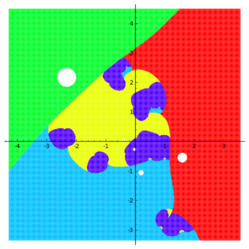
Figure 1. Safes (white disks) and limit areas

In Figure 2, the neighbourhood of the same starting points as in Figure 1 is coloured according to the number of steps until the corresponding Laguerre sequence reaches a safe. Therefore, the areas with the same colour are called “step areas”. If the occurring colours are listed in the order of the rainbow from red to violet, then the index of the colour is the step number. For example, the area surrounding a safe is always red, because one step is needed to enter the safe. Moreover, the second figure shows a trajectory from a starting point to a safe with the maximal number of steps, if the trajectory completely lies in the square.

The arithmetic mean of the roots is given by $\alpha:\,=-\mbox{\raisebox{-0.6pt}{{\large$\frac{1}{m}$}}}c_{m-1}.$ If it fulfills $\sum\limits_{k=1}^{m}\mbox{\raisebox{-0.6pt}{{\large$\frac{1}{\alpha-\varrho_{k}}$}}}\neq 0$ or $\sum\limits_{k=1}^{m}\mbox{\raisebox{-0.6pt}{{\large$\frac{1}{\alpha-\varrho_{k}}$}}}\neq\sum\limits_{k=1}^{m}\mbox{\raisebox{-0.6pt}{{\large$\frac{1}{(\alpha-\varrho_{k})^{2}}$}}},$ which means that $q(\alpha)+s(\alpha)\,r(\alpha)\neq 0,$ and if it lies

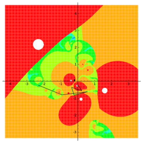
Figure 2. Safes, step areas, a trajectory with maximal step number 7, and the arithmetic mean of the roots (black point)

in the square, then it is shown in the second figure as a black point, because in most cases it is an optimal starting point.

The possibility of selecting arbitrary squares turns the program into a tool. But here, having compared many different figures, we can only state several hypotheses and a conjecture concerning the convergence properties of Laguerre’s method. The corresponding figures with comments and the description of modified programs are contained in a report [7].

• The complex numbers as possible starting points can be divided into four types: inner points, boundary points, “cycle points” which generate cyclic Laguerre sequences and “singularity points” which as starting points are excluded by definition, because they are the multiple zeros of $p^{\prime}(z).$

• The inner points and the boundary points constitute the limit areas and the step areas which both have boundaries consisting of piecewise smooth curves. If there are no singularity points, then a number $S_{p}$ exists such that the starting points of same type with modulus greater than $S_{p}$ form unbounded and simply connected areas. Moreover, each corresponding part of the boundary curve of a limit area or a step area is asymptotic to a straight line.

• The cycle points and the singularity points are the only isolated points.

• The boundary curve of each step area belongs completely or piecewise to one of the neighbouring areas.

• If $\zeta$ is a singularity point or a cycle point, then for each number $N\in\mathbb{N}$ there exists a disk $\Delta_{N}$ with centre $\zeta$ such that the step numbers of all Laguerre sequences with $u_{0}\in\Delta_{N}\setminus\{\zeta\}$ are greater than $N.$

• All Laguerre sequences are bounded. This shall be a conjecture, because, possibly, it can be proved with a method similar to that used for the Theorem above. Namely, in this way, it is easy to show that $\frac{u_{1}}{u_{0}}$ tends to 0 if $u_{0}$ increases unboundedly.

One of the modified programs verifies that it is important to use the sign in the denominator of Laguerre’s method, because without this condition the limit areas and the step areas become highly fragmented. A second program is designed for the positioning of very small squares using the list with the occurring step numbers and turning off the graphics. In this way, for the polynomial $p(z)=z^{5}$ + (0.93 - 0.32 $i$)$z^{4}$ - (0.5818 - 5.8351 $i$)$z^{3}$ - (6.250301 + 1.40811 $i$)$z^{2}$ - (1.61432911 + 2.57707253 $i)z$ + 0.306917325 - 0.531750585 $i,$ which corresponds to the above root list, the (hypothetical) cycle (0.063005…+ 0.1196569…$i$, -0.327219…- 0.4305399…$i$) of length 2 is determined.

References

• [1] Laguerre, E.: Œuvres (Gauthier-Villars, Paris, 1898), Vol. 1 [in French].
• [2] Mekwi, W.: Iterative Methods for Roots of Polynomials. (Master’s thesis, University of Oxford, 2001).
• [3] Möller, H.: Algorithmische Lineare Algebra (Verlag Vieweg, Braunschweig-Wiesbaden, 1997) [in German]. As an e-book available free of charge in [8].
• [4] Möller, H.: An Efficient Reliable Algorithm for the Approximation of All Polynomial Roots Based on the Method of D. Bernoulli. Mathematics and Informatics, 1, Dedicated to the 75th Anniversary of Anatolii Alekseevich Karatsuba, Sovremennye Problemy Matematiki, 16 (2012), Steklov Math. Inst., RAS, Moscow, pp. 52-65. http://mi.mathnet.ru/eng/spm34; last visited: 14 August 2014.
• [5] Möller, H.: An Efficient Reliable Algorithm for the Approximation of All Polynomial Roots Based on the Method of D. Bernoulli. Proceedings of the Steklov Institute of Mathematics, Vol. 280, Suppl. 2 (2013), pp. S43-S55.
• [6] Möller, H.: Laguerre.pyx. Cython program, 2014, available in [8].
• [7] Möller, H.: Report on the Visualization of Laguerre’s Method. 2014, available in [8].
• [8] Möller, H.: http://www.math.uni-muenster.de/u/mollerh/.
• [9] Press, W.H., Teukolsky, S.A., Vetterling, W.T., Flannery, B.P.: Numerical Recipes: The Art of Scientific Computing. (Cambridge University Press, New York, 3rd ed., 2007).
• [10] Stein, W.A., et al.: Sage Mathematics Software (Version 6.1). The Sage Development Team, 2014. http://www.sagemath.org.