Stochastic Local Interaction (SLI) Model: Interfacing Machine Learning and Geostatistics

Abstract

Machine learning and geostatistics are powerful mathematical frameworks for modeling spatial data. Both approaches, however, suffer from poor scaling of the required computational resources for large data applications. We present the Stochastic Local Interaction (SLI) model, which employs a local representation to improve computational efficiency. SLI combines geostatistics and machine learning with ideas from statistical physics and computational geometry. It is based on a joint probability density function defined by an energy functional which involves local interactions implemented by means of kernel functions with adaptive local kernel bandwidths. SLI is expressed in terms of an explicit, typically sparse, precision (inverse covariance) matrix. This representation leads to a semi-analytical expression for interpolation (prediction), which is valid in any number of dimensions and avoids the computationally costly covariance matrix inversion.

I Introduction

Big data is expected to have a large impact in the geosciences given the abundance of remote sensing and earth-based observations related to climate Steed et al. (2013); Addair et al. (2014). A similar data explosion is happening in other scientific and engineering fields Wu et al. (2014). This trend underscores the need for algorithms that can handle large data sets. Most current methods of data analysis, however, have not been designed with size as a primary consideration. This has inspired statements such as: “Improvements in data-processing capabilities are essential to make maximal use of state-of-the-art experimental facilities” Ahrens et al. (2011). Machine learning can extract information and “learn” characteristic patterns in the data. Thus, it is expected to play a significant role in the era of big data research. The application of machine learning methods in spatial data analysis has been spearheaded by Kanevski Kanevski and Maignan (2004). Machine learning and geostatistics are powerful frameworks for spatial data processing. A comparison of their performance using a set of radiological measurements is presented in Giraldi and Bengio (2006). The question that we address in this work is whether we can combine ideas from both fields to develop a computationally efficient framework for spatial data modeling.

Most data processing and visualization methods assume complete data sets, whereas in practice data often have gaps. Hence, it is necessary to fill missing values by means of imputation or interpolation methods. In geostatistics, such methods are based on various flavors of stochastic optimal linear estimation (kriging) Chilès and Delfiner (2012). In machine learning, methods such as $k$-nearest neighbors, artificial neural networks, and the Bayesian framework of Gaussian processes are used Rasmussen and Williams (2006). Both geostatistics and Gaussian process regression are based on the theory of random fields and share considerable similarities Adler (1981); Yaglom (1987). The Gaussian process framework, however, is better suited for applications in higher than two dimensions. A significant drawback of most existing methods for interpolation and simulation of missing data is their poor scalability with the data size $N$, i.e., the $O(N^{3})$ algorithmic complexity and the $O(N^{2})$ memory requirements: An $O(N^{p})$ dependence implies that the respective computational resource (time or memory) increases with $N$ as a polynomial of degree at most equal to $p$.

Improved scaling with data size can be achieved by means of local approximations, dimensionality reduction techniques, and parallel algorithms. A recent review of available methods for large data geostatistical applications is given in Sun et al. (2012). These approaches employ clever approximations to reduce the computational complexity of the standard geostatistical framework. Local approximations involve methods such as maximum composite likelihood Varin et al. (2011) and maximum pseudo-likelihood Van Duijn et al. (2009). Another approach involves covariance tapering which neglects correlations outside a specified range Furrer et al. (2006); Kaufman et al. (2008); Du et al. (2009). Dimensionality reduction includes methods such as fixed rank kriging which models the precision matrix by means of a fixed rank matrix $r\ll N$ Cressie and Johannesson (2008); Nychka et al. (2014). Markov random fields (MRFs) also take advantage of locality using factorizable joint densities. The application of MRFs in spatial data analysis was initially limited to structured grids Rue and Held (2005). However, a recently developed link between Gaussian random fields and MRFs via stochastic partial differential equations (SPDE) has extended the scope of MRFs to scattered data Lindgren and Rue (2011).

We propose a Stochastic Local Interaction (SLI) model for spatially correlated data which is based by construction on local correlations. SLI can be used for the interpolation and simulation of incomplete data in $d$-dimensional spaces, where $d$ could be larger than $3$. The SLI model incorporates concepts from statistical physics, computational geometry, and machine learning. We use the idea of local interactions from statistical physics to impose correlations between “neighboring” locations by means of an explicit precision matrix. The local geometry of the sampling network plays an important role in the expression of the interactions, since it determines the size of local neighborhoods. On regular grids, the SLI model becomes equivalent to a Gaussian MRF with specific structure. For scattered data, the SLI model provides an alternative to the SPDE approach that avoids the preprocessing cost involved in the latter.

The SLI model extends previous research on Spartan spatial random fields Hristopulos (2003); Hristopulos and Elogne (2007); Elogne et al. (2008) to an explicitly discrete formulation and thus enables its application to scattered data without the approximations used in Hristopulos and Elogne (2009). SLI is based on a joint probability density function (pdf) determined from local interactions. This is achieved by handling the irregularity of sampling locations in terms of kernel functions with locally adaptive bandwidth. Kernel methods are common in statistical machine learning (Vapnik, 2000) and in spatial statistics for the estimation of the variogram and the covariance function (Elogne et al., 2008; García-Soidán et al., 2004; Hall et al., 1994).

The remainder of the article is structured as follows: Section II briefly introduces useful definitions and terminology. In Section III we construct the SLI model, propose a computationally efficient parameter estimation approach, and formulate an explicit interpolation expression. In Section IV we investigate SLI interpolation using different types of simulated and real data in one, two and four dimensional Euclidean spaces. Section V discusses potential extensions of the current SLI version and connections with machine learning. Finally, in Section VI we present our conclusions and point to future research.

II Background Concepts and Notation

II.1 Definition of the problem to be learned

Sampling grid

The set of sampling points is denoted by $\textsl{S}_{\rm N}=\{{\bf s}_{1},\ldots,{\bf s}_{N}\}$, where ${\bf s}_{i},$ $i=1,\ldots,N$ are vectors in the Euclidean space $\mathbb{R}^{d}$ or in some abstract feature space that possesses a distance metric. In Euclidean spaces, the domain boundary is defined by the convex hull, ${\mathcal{H}}(S_{N}),$ of $\textsl{S}_{\rm N}.$

Sample and predictions

The sample data are denoted by the vector $\mathbf{x}_{\mathrm{S}}\equiv(x_{1},\ldots,x_{N})^{T}$, where the superscript “$T$” denotes the transpose. Interpolation aims to derive estimates of the observed field at the nodes of a regular grid $\mathcal{G}\subset{\mathbb{Z}}^{d}$, or at validation set points which may be scattered. The estimates (predictions) will be denoted by $\hat{x}({\bf s}_{p})$, $p=1,\ldots,P$, i.e., $\mathbf{\hat{x}}_{\mathrm{P}}=(\hat{x}_{1},\ldots,\hat{x}_{P})^{T}$.

Spatial random field model

The data $\mathbf{x}_{\mathrm{S}}$ are assumed to represent samples from a spatial random field (SRF) $X_{i}(\omega)$, where the index $i=1,\ldots,N$ denotes the spatial location ${\bf s}_{i}\in\textsl{S}_{\rm N}$. The expectation over the ensemble of probable states is denoted by $\mathbb{E}[X_{i}(\omega)]$, and the autocovariance function is given by $C_{i,j}:=\mathbb{E}[X_{i}(\omega)\,X_{j}(\omega)]-\mathbb{E}[X_{i}(\omega)]\,\mathbb{E}[X_{j}(\omega)].$

The pdf of Gibbs SRFs can be expressed in terms of an energy functional $H(\mathbf{x}_{\mathrm{S}};{\bm{\theta}})$, where ${\bm{\theta}}$ is a set of model parameters, according to the Gibbs pdf (Winkler, 1995, p. 51)

$$f_{\rm X}(\mathbf{x}_{\mathrm{S}};{\bm{\theta}})=\frac{\mathrm{e}^{-H(\mathbf{x}_{\mathrm{S}};{\bm{\theta}})}}{Z({\bm{\theta}})}.$$ (1)

The constant $Z({\bm{\theta}})$, called the partition function, is the pdf normalization factor obtained by integrating $\mathrm{e}^{-H(\mathbf{x}_{\mathrm{S}};{\bm{\theta}})}$ over all the probable states $\mathbf{x}_{\mathrm{S}}$.

II.2 From continuum spaces to scattered data

The formulation based on (1) has its origins in statistical physics, and it has found applications in pattern analysis Besag (1974); Geman and Geman (1984) and Bayesian field theory, e.g. Lemm (2005); Farmer (2007). In statistics, this general model belongs to the exponential family of distributions that have desirable mathematical properties Barndorff-Nielsen (2014). Our group used the exponential density in connection with a specific energy functional to develop Spartan spatial random fields (SSRF’s) (Hristopulos, 2003; Hristopulos and Elogne, 2007; Elogne et al., 2008; Hristopulos and Elogne, 2009). In Section III we construct an explicitly discrete model motivated by SSRFs which adapts local interactions to general sampling networks and prediction grids by means of kernel functions.

II.3 Kernel weights

Let $K({\bf r})$ be a non-negative-valued kernel that is either compactly supported or decays exponentially fast at large distances (e.g., the Gaussian or exponential function). We define kernel weights associated with the sampling points ${\bf s}_{i}$ and ${\bf s}_{j}$ as follows

$$K_{i,j}\doteq K\left(\frac{{\bf s}_{i}-{\bf s}_{j}}{h_{i}}\right)=K\left(\frac{\|{\bf s}_{i}-{\bf s}_{j}\|}{h_{i}}\right),$$ (2)

where $\|{\bf s}_{i}-{\bf s}_{j}\|$ is the distance (Euclidean or other) between two points ${\bf s}_{i}$ and ${\bf s}_{j}$, whereas $h_{i}$ is the respective kernel bandwidth that adapts to local variations of the sampling pattern. The kernel weight $K_{j,i}$ is defined in terms of a bandwidth $h_{j}$. Hence, $K_{i,j}\neq K_{j,i}$ if the bandwidths $h_{i}$ and $h_{j}$ are different. Examples of kernel functions are given in Table 1.

Table 1: Definitions of kernel functions used in Section IV below. The first three have compact support. Notation: $u=\|{\bf r}\|/h$ where $\|{\bf r}\|$ is the distance and $h$ the bandwidth; $\mathbbm{1}_{A}(u)$ is the indicator function of the set $A$, i.e., $\mathbbm{1}_{A}(u)=1,\,u\in A$ and $\mathbbm{1}_{A}(u)=0,\,u\notin A.$

Triangular	$K(u)=(1-u)\,\mathbbm{1}_{|u|\leq 1}(u)$
Tricube	$K(u)=(1-u^{3})^{3}\,\mathbbm{1}_{|u|\leq 1}(u)$
Quadratic	$K(u)=(1-u^{2})\,\mathbbm{1}_{|u|\leq 1}(u)$
Gaussian	$K(u)=\exp(-u^{2})$
Exponential	$K(u)=\exp(-|u|)$

Let $D_{i,[k]}(S_{N})$ denote the distance between ${{\bf s}}_{i}$ and its $k$-nearest neighbor in $\textsl{S}_{\rm N}$ $(k=0$ corresponds to zero distance). We choose the local bandwidth associated with ${{\bf s}}_{i}$ according to

$$h_{i}=\mu\,D_{i,[k]}(S_{N}),$$ (3)

where $\mu>1$ and $k>1$ are model parameters. In several case studies involving Euclidean spaces of dimension $d=1,2,3,4$, we determined that $k=2$ (second nearest neighbors) performs well for compactly supported kernels and $k=1$ (nearest neighbors) for infinitely supported kernels. Using $k=2$ for compact kernels avoids zero bandwidth problems which result from $k=1$ for collocated sampling and prediction points. Since the sampling point configuration is fixed, $\mu$ and $D_{i,[k]}(S_{N})$ determine the local bandwidths. $D_{i,[k]}(S_{N})$ depends purely on the sampling point configuration, but $\mu$ also depends on the sample values. For compactly supported kernels setting $k=1$ only makes sense if $\mu>1$; otherwise $h_{i}=D_{i,[k=1]}(S_{N})$ implying that the kernel vanishes even for the nearest-neighbor pairs and thus fails to implement interactions.

II.4 Kernel averages

For any two-point function $\Phi(\cdot)$, we use a local-bandwidth extension of the Nadaraya-Watson kernel-weighted average over the network of sampling points Nadaraya (1964); Watson (1964)

$$\langle\Phi(\cdot)\rangle_{{\bf h}}=\frac{\sum_{i=1}^{N}\sum_{j=1}^{N}K_{i,j}\,\Phi(\cdot)}{\sum_{i=1}^{N}\sum_{j=1}^{N}K_{i,j}},$$

where ${\bf h}=(h_{1},\ldots,h_{N})^{T}$ is the vector of local bandwidths. The function $\Phi(\cdot)$ represents the distance between two points $\|{\bf s}_{i}-{\bf s}_{j}\|$ or the difference $x_{i}-x_{j}$ of the field values, or any other function that depends on the locations or the values of the field. The kernel average is normalized so as to preserve unity, i.e., $\langle 1\rangle_{{\bf h}}=1$ for all possible point configurations.

III The Stochastic Local Interaction (SLI) Model

The SLI joint pdf is determined below by means of the energy functional (4). This leads to a precision matrix which is explicitly defined in terms of local interactions and thus avoids the covariance matrix inversion. The prediction of missing data is based on maximizing the joint pdf of the data and the predictand, which is equivalent to minimizing the corresponding energy functional. This leads to the mode predictor (21), which involves a calculation with linear algorithmic complexity.

III.1 The energy functional

Consider a sample $\mathbf{x}_{\mathrm{S}}$ on an unstructured sampling grid with sample mean $\mu_{\mathrm{X}}$. We propose the following energy functional $H_{\rm X}(\mathbf{x}_{\mathrm{S}};{\bm{\theta}})$

$$H_{\rm X}(\mathbf{x}_{\mathrm{S}};{\bm{\theta}}) =\frac{1}{2\,\lambda\,}\left[{\mathcal{S}_{0}}(\mathbf{x}_{\mathrm{S}})+\,\alpha_{1}\,{\mathcal{S}_{1}}(\mathbf{x}_{\mathrm{S}};{\bf h}_{1})\right.+\left.\alpha_{2}\,{\mathcal{S}_{2}}(\mathbf{x}_{\mathrm{S}};{\bf h}_{2})\right],$$ (4)

where ${\bm{\theta}}=(\mu_{\mathrm{X}},\alpha_{1},\alpha_{2},\lambda,\mu,k)$ is the SLI parameter vector and the parameters $\mu,k$ are defined in Section II.3 above.

The terms $\mathcal{S}_{0}(\mathbf{x}_{\mathrm{S}})$, ${\mathcal{S}_{1}}(\mathbf{x}_{\mathrm{S}};{\bf h}_{1})$, and ${\mathcal{S}_{2}}(\mathbf{x}_{\mathrm{S}};{\bf h}_{2})$ correspond to the averages of the square fluctuations, the square gradient and the square curvature in a Euclidean space of dimension $d$. The latter two are given by kernel-weighted averages that involve the field increments $x_{i,j}=x_{i}-x_{j}$.

$${\mathcal{S}_{0}}(\mathbf{x}_{\mathrm{S}})=\frac{1}{N}\,{\sum_{i=1}^{N}(x_{i}-\mu_{\mathrm{X}})^{2}},$$ (5)

$${\mathcal{S}_{1}}(\mathbf{x}_{\mathrm{S}};{\bf h}_{1})=d\,\langle x_{i,j}^{2}\rangle_{{\bf h}_{1}},$$ (6)

$${\mathcal{S}_{2}}(\mathbf{x}_{\mathrm{S}};{\bf h}_{2})=c_{2,1}\,\langle x_{i,j}^{2}\rangle_{{\bf h}_{2}}-c_{2,2}\,\langle x_{i,j}^{2}\rangle_{{\bf h}_{3}}-c_{2,3}\,\langle x_{i,j}^{2}\rangle_{{\bf h}_{4}},$$ (7a)

$$\mbox{where}\;c_{2,1}=4d(d+2),\;c_{2,2}=2d(d-1),\;c_{2,3}=d.$$ (7b)

The $c_{2,j}$ $(j=1,2,3)$ values in $\mathcal{S}_{2}$ are motivated by discrete approximations of the square gradient and curvature Hristopulos and Elogne (2009). We use two vector bandwidths, ${\bf h}_{1}$ and ${\bf h}_{2}$, to determine the range of influence of the kernel function around each sampling point for the gradient ${\mathcal{S}_{1}}(\mathbf{x}_{n};{\bf h}_{1})$ and curvature ${\mathcal{S}_{2}}(\mathbf{x}_{n};{\bf h}_{2})$ terms respectively. Additional bandwidths used in (7a) for ${\mathcal{S}_{2}}(\mathbf{x}_{n};{\bf h}_{2})$ are defined by ${\bf h}_{3}=\sqrt{2}\,{\bf h}_{2}$, ${\bf h}_{4}=2\,{\bf h}_{2}.$ These definitions are motivated by the formulation of SSRFs Hristopulos (2003); Hristopulos and Elogne (2009).

III.2 SLI parameters and permissibility

To obtain realistic kernel bandwidths, $k$ should be a positive integer larger than one, and $\mu$ should be larger than one. The parameter $\mu_{\rm X}$ is set equal to the sample mean. The coefficients $\alpha_{1},\alpha_{2}$ control the relative contributions of the mean square gradient and mean square curvature terms. The coefficient $\lambda$ controls the overall amplitude of the fluctuations. Finally, $\mu$ and $k$ control the bandwidth values as described in Section II.3.

The SLI energy functional (4) is permissible if $H_{\rm X}(\mathbf{x}_{\mathrm{S}};{\bm{\theta}})\geq 0$ for all $\mathbf{x}_{\mathrm{S}}$, a condition which ensures that $\mathrm{e}^{-H(\mathbf{x}_{\mathrm{S}};{\bm{\theta}})}$ is bounded and thus the existence of the partition function in (1). Assuming that $\mathcal{S}_{2}\geq 0$ ($\mathcal{S}_{0}$ and $\mathcal{S}_{1}$ are always non-negative by construction), a sufficient permissibility condition, independently of the distance metric used, is $\alpha_{1},\alpha_{2},\lambda>0$. In all the case studies that we have investigated, however, we have not encountered permissibility problems so long as $\alpha_{1},\alpha_{2},\lambda>0$. Intuitively, the justification for the permissibility of (4) is that the first average, i.e., $\langle x_{i,j}^{2}\rangle_{{\bf h}_{2}}$ in (7a) has a positive sign and is multiplied by $c_{2,1}$, which is significantly larger (especially as $d$ increases) than the coefficients $c_{2,2}$ and $c_{2,3}$ multiplying the negative-sign averages $\langle x_{i,j}^{2}\rangle_{{\bf h}_{3}}$ and $\langle x_{i,j}^{2}\rangle_{{\bf h}_{4}}$. This property is valid for geodesic distances on the globe and for other metric spaces as well.

III.3 Precision matrix representation

We express (4) in terms of the precision matrix $\hat{J}_{i,j}({\bm{\theta}})$ ($i,j=1,\ldots,N$)

$$H_{\rm X}(\mathbf{x}_{\mathrm{S}};{\bm{\theta}})=\frac{1}{2}(\mathbf{x}_{\mathrm{S}}-\bm{\mu}_{\mathrm{X}})^{T}\,{\mathbf{J}}({\bm{\theta}})\,(\mathbf{x}_{\mathrm{S}}-\bm{\mu}_{\mathrm{X}}).$$ (8)

The symmetric precision matrix ${\mathbf{J}}({\bm{\theta}})$ follows from expanding the squared differences in (4), leading to the following expression

$${\mathbf{J}}({\bm{\theta}})=\frac{1}{\lambda} \,\left\{\frac{{\bf I}_{N}}{N}+\alpha_{1}\,d\,{\mathbf{J}}_{1}({{\bf h}}_{1})+\alpha_{2}\,\left[c_{2,1}\,{\mathbf{J}}_{2}({{\bf h}}_{2})-c_{2,2}\,{\mathbf{J}}_{3}({{\bf h}}_{3})-c_{2,3}\,{\mathbf{J}}_{4}({{\bf h}}_{4})\right]\right\},$$ (9)

where ${\bf I}_{N}$ is the $N\times N$ identity matrix: $[{\bf I}_{N}]_{i,j}=1$ if $i=j$ and $[{\bf I}_{N}]_{i,j}=0$ otherwise, and ${\mathbf{J}}_{q}({{\bf h}}_{q}),\;q=1,2,3,4$ are network matrices that are determined by the sampling pattern, the kernel function, and the bandwidths. The index $q$ defines the gradient network matrix for $q=1$, whereas the values $q=2,3,4$ specify the curvature network matrices that correspond to the three terms in ${\mathcal{S}_{2}}(\mathbf{x}_{\mathrm{S}};{\bf h}_{2})$ given by (7a). The elements of the network matrices ${\mathbf{J}}_{q}({\bf h}_{q})$ are given by the following equations

$$[{\mathbf{J}}_{q}({{\bf h}}_{q})]_{i,j} =-u_{i,j}(h_{q;i})-u_{i,j}(h_{q;j})+[{\bf I}_{N}]_{i,j}\,\sum_{l=1}^{N}\left[u_{i,l}(h_{q;i})+u_{l,i}(h_{q;l})\right],$$ (10a)

$$u_{i,j}(h_{q;i}) =\frac{K\left(\frac{{\bf s}_{i}-{\bf s}_{j}}{h_{q,i}}\right)}{\sum_{i=1}^{N}\sum_{j=1}^{N}K\left(\frac{{\bf s}_{i}-{\bf s}_{j}}{h_{q,i}}\right)},\quad q=1,\ldots,4.$$ (10b)

The network matrices defined by (10) are symmetric by construction. It follows from (10) that the row and column sums vanish, i.e.,

$$\sum_{j=1}^{N}[{\mathbf{J}}_{q}({{\bf h}}_{q})]_{i,j}=0.$$ (11)

Based on (10a), the diagonal elements are given by the following expression

$$[{\mathbf{J}}_{q}({{\bf h}}_{q})]_{i,i}=\sum_{l=1,\neq i}^{N}\left[u_{i,l}(h_{q;i})+u_{l,i}(h_{q;l})\right].$$ (12)

Since the kernel weights are non-negative, it follows that the sub-matrices ${\mathbf{J}}_{q}({{\bf h}}_{q})$ are diagonally dominant, i.e., $\big{|}[{\mathbf{J}}_{q}({{\bf h}}_{q})]_{i,i}\big{|}\geq\sum_{j\neq i}\big{|}[{\mathbf{J}}_{q}({{\bf h}}_{q})]_{i,j}\big{|}$. It also follows from (9) and (11) that

$$\sum_{j=1}^{N}[{\mathbf{J}}({\bm{\theta}})]_{i,j}=\frac{1}{N\lambda}.$$ (13a)

III.4 Parameter inference

We have experimented both with maximum likelihood estimation and leave-one-out cross validation. The former requires the calculation of the SLI partition function, which is an $O(N^{3})$ operation for scattered data. For large data sets the $O(N^{3})$ complexity is a computational bottleneck. Parameter inference by optimization of a cross validation metric is computationally more efficient, since it is at worst an $O(N^{2})$ operation as we show below. The memory requirements for storing the precision matrix are $O(N^{2})$ but can be significantly reduced by using sparse matrix structures. Let ${\bm{\theta}}_{-\lambda}=(\alpha_{1},\alpha_{2},\mu,\mu_{\mathrm{X}})^{T}$ represent the parameter vector excluding $\lambda$. We use the following cross validation cost functional

$$\Phi(\mathbf{x}_{\mathrm{S}};{\bm{\theta}}_{-\lambda})=\sum_{i=1}^{N}|\hat{x}_{i}({\bm{\theta}}_{-\lambda})-x_{i}\,|,$$ (14)

where $\hat{x}_{i}({\bm{\theta}}_{-\lambda})$ is the SLI prediction at ${\bf s}_{i}$ based on the reduced sampling set $\textsl{S}_{\rm N}-\{{\bf s}_{i}\}$ using the parameter vector ${\bm{\theta}}_{-\lambda}$ which applies to all $i=1,\ldots,N$. The prediction is based on the interpolation equation (III.5.2) below and does not involve $\lambda$ (see discussion in Section V.2).

The optimal parameter vector excluding $\lambda$, i.e., ${\bm{\theta}}_{-\lambda}$, is determined by minimizing the cost functional (14):

$${\bm{\theta}}^{\ast}_{-\lambda}=\arg\min_{{\bm{\theta}}_{-\lambda}}\Phi(\mathbf{x}_{\mathrm{S}};{\bm{\theta}}_{-\lambda}).$$ (15)

If $\tilde{H}(\mathbf{x}_{\mathrm{S}};{\bm{\theta}}_{-\lambda})$ is the energy estimated from (8) and (9) by setting $\lambda=1$, the optimal value $\lambda^{\ast}$ is obtained by minimizing the negative log-likelihood with respect to $\lambda$ leading to the following solution (see A)

$$\lambda^{\ast}=\frac{2\tilde{H}(\mathbf{x}_{\mathrm{S}};{\bm{\theta}}_{-\lambda})}{N}.$$ (16)

We determine the minimum of the cross validation cost functional (14) using the Matlab constrained optimization function fmincon with the interior-point algorithm Wright (2005). This function determines the local optimum nearest to the initial parameter vector. We use initial guesses for the parameters $\alpha_{1},\alpha_{2},\mu$, and we assume that the parameters are constrained between the lower bounds $[0.5,0.5,0.5]$ and the upper bounds $[300,300,15]$. We investigated different initial guesses for the parameters which led to different local optima. We found, however, that the value of the cross validation function is not very sensitive on the local optimum. In the $4D$ case study presented in Section IV.2, we also estimate for comparison purposes the global optimum using Matlab’s global optimization tools.

III.5 Predictive SLI model

Let us now assume that the prediction point ${\bf s}_{p}$ is added to the sampling points. To predict the unknown value of the field at ${\bf s}_{p}$, we insert this point in the energy functional (8), which is then given by Eq. (III.5.2) below. Then, we determine the mode of the joint pdf (1) with the prediction point inserted in the energy functional. Thus, we obtain a mode prediction equation for $\hat{x}_{p}$ given by (III.5.2) below.

III.5.1 Modification of kernel weights

Upon inclusion of ${\bf s}_{p}$, the weights (10b) of the network matrices (10a) are modified as follows

$$u_{i,j}(h_{q;i})=\frac{K\left(\frac{{\bf s}_{i}-{\bf s}_{j}}{h_{q,i}}\right)}{\sum_{i,j}K\left(\frac{{\bf s}_{i}-{\bf s}_{j}}{h_{q,i}}\right)+\sum_{i}K\left(\frac{{\bf s}_{i}-{\bf s}_{p}}{h_{q,i}}\right)+\sum_{i}K\left(\frac{{\bf s}_{i}-{\bf s}_{p}}{h_{q,p}}\right)},$$ (17)

where $\sum_{i,j}:=\sum_{i=1}^{N}\sum_{j=1}^{N}$. The first term in the denominator concerns interactions between sampling points. The second term involves local interactions between the sampling points and the prediction point which result from inserting the prediction point in the local neighborhoods of the sampling points, which control the bandwidths. Finally, the third term also involves interactions between the prediction point and the sampling points, but in this case the bandwidth is controlled by the former. Fig. 1 below illustrates the difference between the second and third term in the context of the entire precision matrix. The index $q$ is used to distinguish between the weights linked to the gradient $(q=1)$ and the three weights $(q=2,3,4)$ linked to the curvature terms. The only difference between weights with different $q$ is the bandwidth. In the case of compactly supported kernels, different bandwidths imply that different numbers of pairs are involved in the summations, since a pair separated by a distance that exceeds the bandwidth does not contribute. Calculation of the predictand contributions in the denominator of (17) is an operation with computational complexity $O(N)$ compared to $O(N^{2})$ for the interactions between sampling points. The latter term, however, is calculated once and used for all the prediction points.

In addition to the weights that correspond to pairs of sampling points, there are weights for combinations of sampling and prediction points, i.e.,

$$u_{p,j}(h_{q;p})=\frac{K\left(\frac{{\bf s}_{p}-{\bf s}_{j}}{h_{q,p}}\right)}{\sum_{i,j}K\left(\frac{{\bf s}_{i}-{\bf s}_{j}}{h_{q,i}}\right)+\sum_{i}K\left(\frac{{\bf s}_{i}-{\bf s}_{p}}{h_{q,i}}\right)+\sum_{i}K\left(\frac{{\bf s}_{i}-{\bf s}_{p}}{h_{q,p}}\right)},$$ (18)

where $p=1,\ldots,P$, $j=1,\ldots,N$. The denominator of (18) is identical to that of (17).

III.5.2 SLI mode predictor

Using the precision matrix formulation, the energy functional including the predictand is given by

$${\hat{H}_{\rm X}}(\mathbf{x}_{\mathrm{S}},x_{p};{\bm{\theta}}^{\ast})= H_{\rm X}(\mathbf{x}_{\mathrm{S}};{\bm{\theta}}^{\ast})+J_{p,p}({\bm{\theta}}^{\ast})(x_{p}-\mu_{\mathrm{X}})^{2}+\sum_{i=1}^{N}(x_{i}-\mu_{\mathrm{X}})\,J_{i,p}({\bm{\theta}}^{\ast})\,(x_{p}-\mu_{\mathrm{X}})$$

$$+\sum_{i=1}^{N}(x_{p}-\mu_{\mathrm{X}})\,J_{p,i}({\bm{\theta}}^{\ast})\,(x_{i}-\mu_{\mathrm{X}}).$$ (19)

The elements of the precision matrix that involve the prediction point are

$$[{\mathbf{J}}_{q}({{\bf h}}_{q})]_{p,p}= \sum_{i=1}^{N}\left[u_{i,p}(h_{q;i})+u_{p,i}(h_{q;p})\right],$$ (20a)

$$[{\mathbf{J}}_{q}({{\bf h}}_{q})]_{i,p}= -\left[u_{i,p}(h_{q;i})+u_{p,i}(h_{q;p})\right],\;i\neq p.$$ (20b)

Based on (20a) the symmetry property $J_{p,i}({\bm{\theta}}^{\ast})=J_{i,p}({\bm{\theta}}^{\ast})$ follows. The coefficients $u_{i,p}(h_{q;i})$ and $u_{p,i}(h_{q;p})$ differ due to the different bandwidths used (in the former, the bandwidth is determined by the neighborhood of the sampling point ${\bf s}_{i}$, whereas in the latter by the neighborhood of ${\bf s}_{p}$.) A schematic illustration of terms in (III.5.2) that involve the predictand is given in Fig. 1. The left diagram corresponds to terms “rooted” at ${\bf s}_{p}$ (i.e., with coefficient $u_{p,i}(h_{q;p})$ that involves the bandwidth $h_{p}$), whereas the right hand side diagram corresponds to terms rooted at the sampling points, i.e., with coefficients $u_{i,p}(h_{q;i})$.

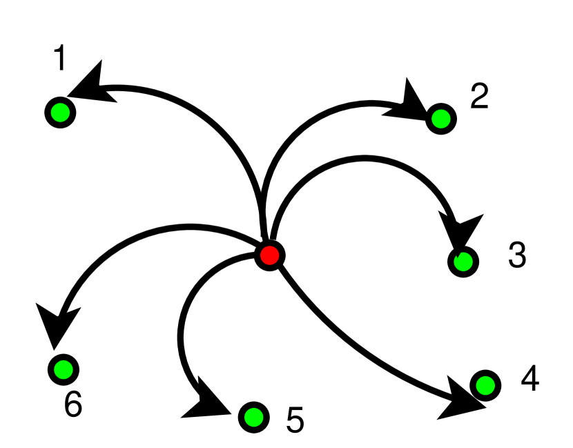
(a) Bandwidth determined by ${\bf s}_{p}$.

(b) Bandwidth determined by ${\bf s}_{n}$.

Figure 1: Schematic diagrams of terms contributing to (III.5.2) that include the prediction point ${\bf s}_{p}$ (center point) and six sampling points ${\bf s}_{n}$ $(n=1,\ldots,6)$. The diagram on the left (a) represents terms $J_{p,i}$ whereas the diagram on the right (b) represents terms $J_{i,p}$. The point at the “root” of each arrow determines the bandwidth for the weight that involves the two points connected by the arrow.

The SLI mode predictor is defined by the following equation

$$\hat{x}_{p}=\arg\min_{x_{p}}{\hat{H}_{\rm X}}(\mathbf{x}_{\mathrm{S}},x_{p};{\bm{\theta}}^{\ast}),$$ (21)

where ${\hat{H}_{\rm X}}(\mathbf{x}_{\mathrm{S}},x_{p};{\bm{\theta}}^{\ast})$ is given by (III.5.2). Minimization of the energy with respect to $x_{p}$ leads to the following mode estimator

$$\hat{x}_{p} =\mu_{\mathrm{X}}-\frac{\sum_{i=1}^{N}\,\left[J_{i,p}({\bm{\theta}}^{\ast})+J_{p,i}({\bm{\theta}}^{\ast})\right]\,(x_{i}-\mu_{\mathrm{X}})}{2\,J_{p,p}({\bm{\theta}}^{\ast})}$$

$$=\mu_{\mathrm{X}}-\frac{\sum_{i=1}^{N}\,J_{p,i}({\bm{\theta}}^{\ast})\,(x_{i}-\mu_{\mathrm{X}})}{J_{p,p}({\bm{\theta}}^{\ast})},$$ (22)

where the precision matrix elements are given by (10a) using the modified kernel weights (17) and (18).

The SLI mode predictor can be generalized to $P$ prediction points as follows

$$\mathbf{\hat{x}}_{p}=\bm{\mu}_{\mathrm{X}}-\mathbf{\tilde{J}}_{P,S}({\bm{\theta}}^{\ast})\,(\mathbf{x}-\bm{\mu}_{\mathrm{X}}),$$ (23a)

where $\mathbf{\tilde{J}}_{P,S}({\bm{\theta}}^{\ast})$ is a $P\times N$ matrix given by

$$[\mathbf{\tilde{J}}_{P,S}({\bm{\theta}}^{\ast})]_{p,i}=J_{p,i}({\bm{\theta}}^{\ast})/J_{p,p}({\bm{\theta}}^{\ast}).$$ (23b)

III.5.3 Properties of SLI predictor

The SLI prediction (23) is unbiased in view of the vanishing row sum property (13a) satisfied by the network matrices and the precision matrix. The SLI prediction (23) is independent of the parameter $\lambda$ which sets the amplitude of the fluctuations, because the transfer matrix $\mathbf{\tilde{J}}_{P,S}({\bm{\theta}}^{\ast})$ is given by the ratio of precision matrix elements. This property is analogous to the independence of the kriging predictor from the random field variance. Hence, leave-one-out cross validation does not determine the optimal value of $\lambda$, which is obtained from (16).

The SLI predictor is not necessarily an exact interpolator. In particular, let us consider a point ${\bf s}_{k}$, $k\in\{1,\ldots,N\}$, which is very close to ${\bf s}_{p}$. Based on (20) and (III.5.2), $\hat{x}_{p}\rightarrow x_{k}$ as ${\bf s}_{p}\rightarrow{\bf s}_{k}$ only if (i) $|u_{k,p}(h_{p})|\gg|u_{i,p}(h_{p})|$ and (ii) $|u_{k,p}(h_{k})|\gg|u_{i,p}(h_{i})|$ for all $i\neq k$. Condition (i) materializes only for compactly supported kernels if $h_{p}\rightarrow 0$ which requires that the bandwidth be determined by the nearest neighbor distance. Condition (ii), on the other hand, requires that $\|{\bf s}_{k}-{\bf s}_{p}\|/h_{k}\ll\|{\bf s}_{i}-{\bf s}_{p}\|/h_{i}$ for $i\neq k.$ This condition holds approximately at best if the sample is sparse around ${\bf s}_{p}$.

The computational complexity of the SLI predictor is $O(N^{2}+P\,N)$. The $O(N^{2})$ term is due to the double summation over the sampling points in (17), which needs to be calculated only once. The remaining operations per each prediction point scale linearly with the sample size, hence the $O(P\,N)$ dependence. Based on the above, the dominant term (for fixed $P$) in the computational time scales as $O(N^{2})$. In future work we will investigate approximating the double summation in the denominator of (10b) and (18) with analytically evaluated double integrals over the kernel functions to increase the computational efficiency.

IV Case Studies

We first consider two synthetic data sets, the first consisting of a time series and the second of a four-dimensional test function. We then investigate a set of scattered real data in two spatial dimensions.

IV.1 Time series with Matérn covariance function

We generate a time series of length $N=300$ from a random process with Matérn covariance $C(\tau)=\sigma^{2}\,2^{1-\nu}K_{\nu}(\tau/\xi)(\tau/\xi)^{\nu}/\Gamma(\nu)$, where $K_{\nu}(\cdot)$ is the modified Bessel function of order $\nu$, $\Gamma(\cdot)$ is the gamma function, $\sigma=10$, $\nu=3.5$ is the smoothness index, and $\xi=10$ is the correlation time. We use 60 randomly selected points as the training set (corresponding to an $80\%$ degree of thinning) and the remaining 240 points as the validation set. The SLI optimal parameters using a quadratic kernel and $k=2$ are given by $\alpha_{1}\approx 29.30,\alpha_{2}\approx 191.02,\mu\approx 1.11,\lambda\approx 297.84$. The sparseness of the precision matrix is evident in Fig. 2(a). The darkest areas correspond to negative infinity and reflect distances for which the precision matrix vanishes.

The prediction performance is illustrated in the scatter plot of the SLI predictions versus the respective validation set values shown in Fig. 2(b). The Pearson correlation coefficient between the validation values and the predictions is $0.89.$ The splitting of the time series into training and validation sets is shown in Fig. 3 along with the SLI predictions and associated error bars. The SLI predictions capture well general features of the time series. However, in areas of low sampling density the SLI predictions smoothes excessively the fluctuations in the original series. The SLI performance is excellent for the same degree of thinning, if the length of the initial time series increases to $3\,000$. On the other hand, the prediction accuracy deteriorates for rougher random processes, such as a non-differentiable Matérn process with $\nu=0.8$.

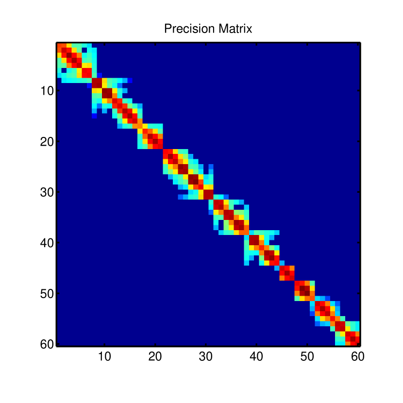
(a) $\ln|J_{i,j}|$

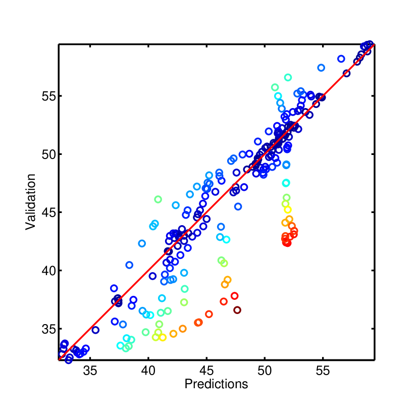
(b) Predictions vs validation values

Figure 2: Analysis of time series with Matérn correlations ($\sigma=10$, $\nu=3.5$, $\xi=10$). (a) Logarithm of absolute value of the precision matrix; dark areas (blue online) correspond to low values whereas lighter areas (green to red online) correspond to higher values. (b) Scatter plot of SLI predictions versus the respective values of the validation set.

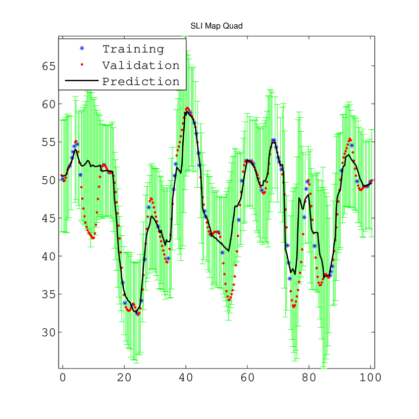
Figure 3: SLI predictions at 240 validation points of time series with Matérn correlations ($\sigma=10$, $\nu=3.5$, $\xi=10$). The 60 training points are marked by stars (blue online), validation points are marked by dots (red online), and SLI predictions are marked by the continuous line (black online). Error bars are based on three times the conditional standard deviation (green online).

IV.2 Four-dimensional deterministic test function

We consider the function $x({\bf s})$

$$x({\bf s})=A\,{\rm e}^{-2\|{\bf s}-{\mathbf{a}}\|}\,\prod_{i=1}^{4}s_{i}\,(1-s_{i}),$$ (24)

where $A=500$ and $\mathbf{a}=(0.3,0.3,0.3,0.3)$, defined over the four-dimensional cube with unit length edges, i.e., for ${\bf s}\in[0,1]^{4}$. We sample the function at $N=1\,000$ randomly selected points over the unit cube, and we generate a validation set of $N=1\,000$ points also by random selection. The SLI optimal parameters for the quadratic kernel with $k=2$ are given by $\alpha_{1}\approx 10.12,\alpha_{2}\approx 25.04,\mu\approx 1.64,\lambda\approx 0.0193$ starting with initial values $\alpha_{1}=10,\alpha_{2}=25,\mu=3$. Similar results in terms of cross validation performance are also obtained with different initial conditions that lead to different local optima. The cross validation measures for the parameters above are given by ME$=0.0046$, MAE$=0.0320$, RMSE$=0.0459$, $r$$=0.96$. The sparse structure of the precision matrix is illustrated in Fig. 4(a) which displays the logarithm of the absolute value. The scatter plot of the validation values versus the respective SLI predictions is shown in Fig. 4(b) and demonstrates very good agreement at most points.

We repeat the experiment by adding Gaussian noise to the sample. The standard deviation of the noise is set to $\approx 10\%$ of the maximum sampled value $x_{\max}$ (in the simulations that we ran $x_{\max}\approx 1$). While the coefficients $\alpha_{1}$ and $\alpha_{2}$ remain practically unchanged, $\mu$ changes to $\approx 1.83$. The sparsity of the precision matrix is $\approx 76\%$. The respective cross validation measures are given by ME$=0.012$, MAE$=0.047$, RMSE$=0.061$, and $r$$=0.93$.

We also used the Matlab global optimizer GlobalSearch with the same initial parameter vector as above to determine the SLI model parameters. GlobalSearch uses a scatter-search algorithm to generate starting points (initial parameter guesses). The minimization is conducted using fmincon to determine the local minimum close to the current starting point. We use the lower and upper bounds defined in Section III.4 to constrain the space of the starting points. GlobalSearch investigates a set of 66 starting points, and convergence to a local minimum is achieved for all of them. The globally optimal SLI parameters are estimated as $\alpha_{1}\approx 1.50,\alpha_{2}\approx 224.62,\mu\approx 2.01,\lambda\approx 0.748$. The respective validation measures are given by ME$=0.0055$, MAE$=0.045$, RMSE$=0.063$, and $r=0.93$. These measures do not differ significantly from those obtained with the locally optimum solution. The MAE value is lower for the global optimum, which is expected since MAE reflects the value of the cost function (14). On the other hand, the RMSE obtained with the global optimum is slightly higher than that of the local optimum. This result indicates that quite different parameter vectors can lead to similar cross validation results. This behavior has also been observed with covariance models whose parameter vector involves more than the variance and the correlation length Žukovič and Hristopulos (2009); Hristopulos and Žukovič (2011).

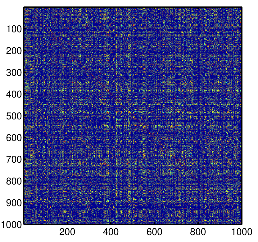
(a) $\ln|J_{i,j}|$

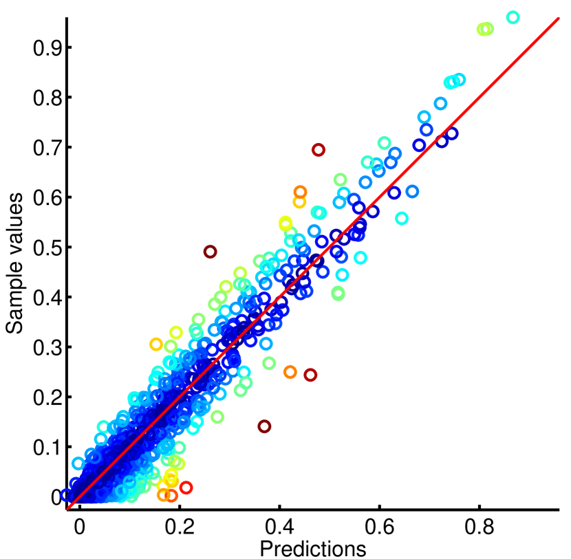
(b) Predictions vs validation values

Figure 4: Analysis of the truncated exponential function (24). (a) Logarithm of the absolute value of the precision matrix; dark areas (blue online) correspond to low values whereas lighter areas (green to red online) correspond to higher values. (b) Scatter plot of SLI predictions versus the respective values of the validation set.

IV.3 Radioactivity data in two dimensions

This example focuses on daily means of radioactivity gamma dose rates over part of the Federal Republic of Germany. The data were provided by the German automatic radioactivity monitoring network for the Spatial Interpolation Comparison Exercise 2004 (SIC 2004) Dubois and Galmarini (2006). This data set is well studied and thus allows easy comparisons with other methods Elogne et al. (2008). The $1\,008$ stations are partitioned into a training set of $200$ randomly selected locations and a validation set of $808$ locations where predictions are compared with the observations. Two different scenarios are investigated: A normal data set corresponding to typical background radioactivity measurements, and an emergency data set, in which a local release of radioactivity in the southwest corner of the monitored area was simulated using a dispersion process to obtain a few values with magnitudes around 10 times higher than the background. The rates are measured in nanoSievert per hour (nSv/h). The normal training set follows the Gaussian distribution with the minimum around 58 nSv/h and the maximum around 153 nSv/h. In the emergency training set there are two values $>1\,000$ nSv/h, with the maximum at $1\,499$ nSv/h. We compare the prediction performance of the SLI model against the $808$ values of the validation set.

IV.3.1 Normal data

For normal data, the optimal SLI parameters based on the training set with a quadratic kernel and $k=2$ are given by $\alpha_{1}\approx 143,\alpha_{2}\approx 47.56,\mu\approx 2.64,\lambda\approx 3.24\times 10^{3}$. Figure 5(a) illustrates the relative values of the bandwidths used. Higher values correspond to more isolated points in areas of low sampling density and along the boundaries of the convex hull of the domain. Figure 5(b) presents the natural logarithm of the absolute value of the precision matrix. Overall, about $32\%$ (i.e., 12 718) of the total number of pairs yield nonzero precision values, implying that the sparsity of the precision matrix is $\approx 68\%$.

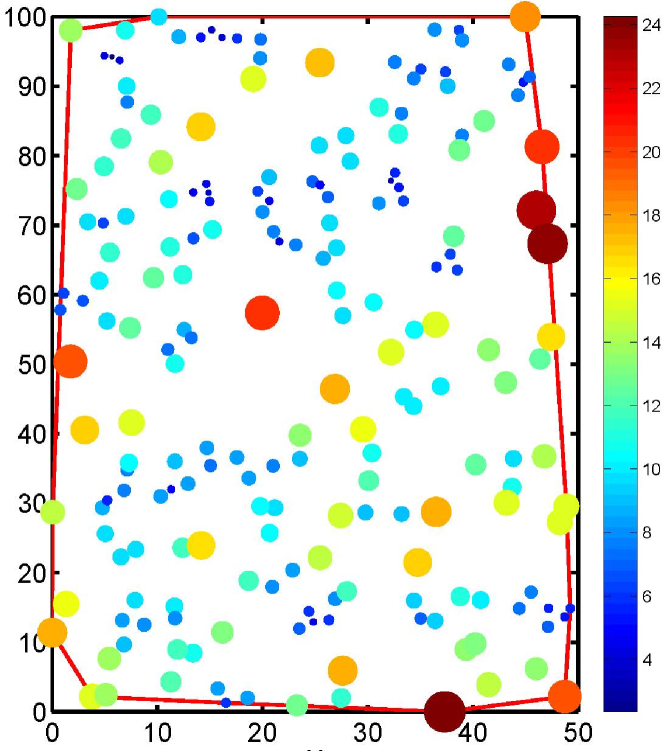
(a) Relative bandwidth

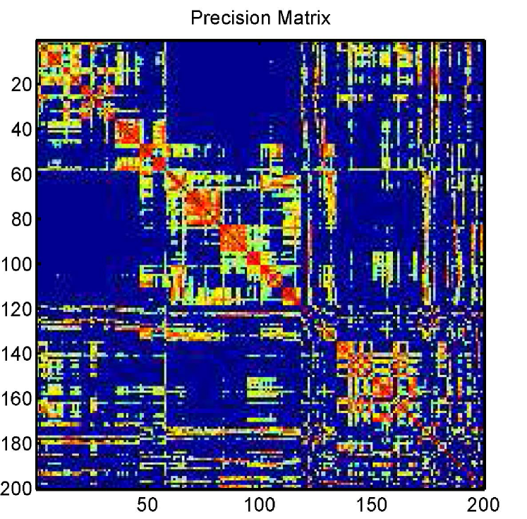
(b) $\ln|J_{i,j}|$

Figure 5: Analysis of SIC 2004 normal data set using normalized coordinates; the longest side is set to 100 and the aspect ratio is maintained. (a) Bubble plot of the relative size of local bandwidths: larger circles correspond to bigger bandwidths. The continuous line along the domain boundary marks the convex hull of the sampling set. (b) Logarithm of the absolute values of the precision matrix elements. Darker areas (blue online) correspond to lower values, whereas lighter areas (red online) correspond to higher values.

The cross-validation results are tabulated in Table 2. The cross validation measures (based on the validation set) obtained in a recent study by means of Ordinary Kriging are: ME$=-1.36$, MAE$=9.29$, RMSE$=12.59$, $r$$=0.78$ Elogne et al. (2008). These values are in close agreement with the SLI results in Table 2.

Various geostatistical and machine learning methods have been applied to the SIC 2004 data (neural networks, geostatistics, and splines). Excluding the results of some poor performers, the cross validation measures obtained are in the following ranges Dubois and Galmarini (2006): ME $\in[-1.39,-0.04]$ and $\in[0.20,1.60]$, MAE $\in[9.05,12.10]$, RMSE $\in[12.43,15.90]$, and $r$ $\in[0.64,0.79]$. Hence, the SLI cross validation results are close to the best performers. Fig. 6 presents a map of the radioactivity pattern generated by SLI and contrasts it with the map generated by bilinear interpolation. The SLI spatial pattern is smoother and thus appears more realistic. Its smoothing effect near the sample values, however, is more pronounced than that caused by bilinear interpolation.

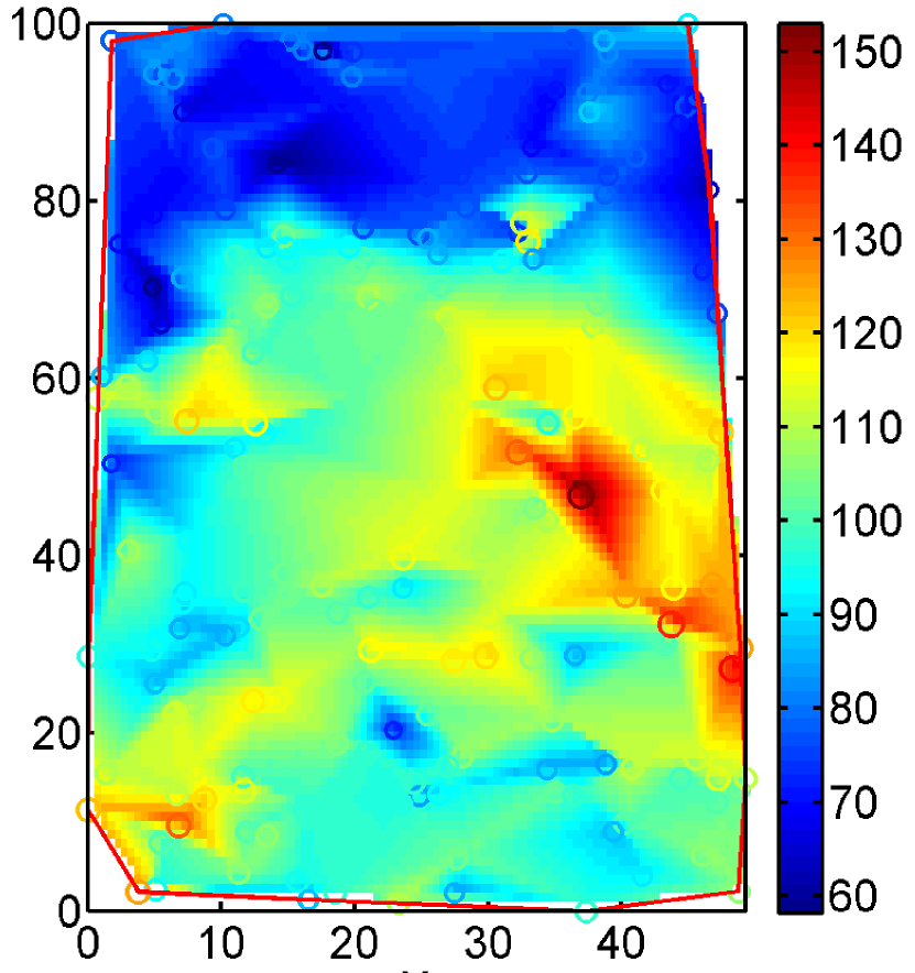
(a) Bilinear interpolation

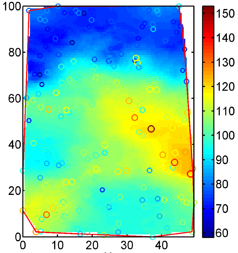
(b) SLI interpolation

Figure 6: Map of background radioactivity rates in Germany (based on 200 training data) using a mapping grid with $100$ nodes per side. (a) Bilinear interpolation using the griddata command of Matlab. (b) SLI interpolation map using the optimal parameters reported in the text.

Table 2: Cross validation performance measures for SIC 2004 normal data. The second row presents the performance of the SLI predictor at the 808 validation set points. ME: Mean error (bias); MAE: Mean absolute error; MARE: Mean absolute relative error; RMSE: Root mean square error; $r$: Pearson correlation coefficient.

SLI	ME	MAE	MARE	RMSE	$r$
Validation set	$-$1.30	9.30	0.09	12.62	0.78

We also conduct a stability analysis by removing one sampling point at a time and determining the optimal SLI model using leave-one-out cross validation with that point removed. The variation of the SLI parameters is shown in Fig. 7; $\alpha_{1},\alpha_{2}$ and $\mu$ are quite stable, whereas $\lambda$ shows more variability. The spikes in the plots of Fig. 7 are exaggerated by using a narrow vertical range to better illustrate the parameter variability. For $\alpha_{1}$, $\alpha_{2}$ the maximum relative variation (with respect to the mean) ranges from a fraction of a thousandth (for $\alpha_{1}$) to few thousandths (for $\alpha_{2}$); $\mu$ shows stronger variations, whereas the strongest variation is exhibited by $\lambda$, since the latter is a scaling factor that determines the overall energy of the ensemble of points and compensates for variations in the other parameters. We believe that the parameter variations exhibited in Fig. 7 are, at least partially due to extremely slow variation of the cost function over a region of the parameter space, a condition also observed in maximum likelihood estimation of spatial models with Matérn covariance Žukovič and Hristopulos (2009). This slow variation implies quasi-degeneracy of the parameter vector; the quasi-degeneracy implies that vectors which are very far in parameter space may lead to very similar cost function values. More recently, the difficulties involved in nonlinear fits of multi-parametric models to data have been investigated in Transtrum et al. (2010).

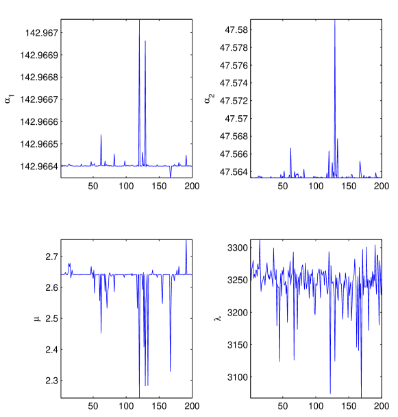
Figure 7: Variation of SLI parameters estimated by removing one value at a time from the 200 training locations of the SIC 2004 normal data.

IV.3.2 Emergency data

For the SIC 2004 emergency data, cross validation results with different kernel functions (tricubic, exponential, and quadratic) are shown in Table 3. The SLI parameters are initialized using the optimal values for the normal data. The last row of the table is based on estimation with a quadratic kernel function after removing the three highest values. The best results in Table 3 are obtained with the quadratic kernel including all the data. The optimal SLI parameters are $\alpha_{1}\approx 143,\alpha_{2}\approx 47.56,\mu\approx 2.69,\lambda\approx 4.32\times 10^{5}$. The parameters, except for $\lambda$, are close to their normal case counterparts. The difference in $\lambda$ is due to the much higher variance of the emergency data set.

The variation of the SLI parameters in leave-one-out cross validation exhibits similar patterns as for the normal data, except that more pronounced variations of $\lambda$ are observed when the extreme values are removed. The precision matrix has 23 232 non-zero elements, implying a sparsity of $\approx 42\%$, in contrast with 12 718 (sparsity $\approx 32\%$) in the normal case. This difference clearly illustrates the dependence of the precision matrix on the sample values in addition to the sampling pattern. SLI does not rely on estimating the variogram function, and thus it is not hindered by the presence of extreme values. On the other hand, geostatistical methods rely on the variogram function, which may not be reliably estimated in such cases Giraldi and Bengio (2006). The Pearson correlation coefficient is significantly lower than in the normal set due to underestimation of the extreme values, while the Spearman rank correlation coefficient is comparable to the normal case. The cross validation measures obtained in SIC 2004 are in the following intervals Dubois and Galmarini (2006): ME $\in[-11.10,-0.12]$ and $\in[0.41,19.71]$, MAE $\in[14.85,146.36]$, RMSE $\in[45.46,212.10]$, and $r$ $\in[0.02,0.86]$. The best performance in terms of both MAE and RMSE was obtained by means of a Generalized Regression Neural Network Timonin and Savelieva. (2006). Looking at the scatter plot of MAE versus RMSE —Fig. 6 in Dubois (1998)— the SLI performance is closer to the geostatistical and spline methods.

Table 3: SLI cross validation performance measures for SIC 2004 emergency data. The second row presents the performance of the SLI predictor at the 808 validation set points. The first five cross validation measures are as described in the caption of Table 2, and $r_{S}$ is the Spearman correlation coefficient.

SLI Kernel function	ME	MAE	MARE	RMSE	$r$	$r_{S}$
Tricubic: $(1-u^{3})^{3}$	5.78	24.22	0.20	81.33	0.25	0.57
Exponential: ${\mathrm{e}}^{-u}$	6.06	23.84	0.19	79.78	0.34	0.63
Quadratic	3.04	23.16	0.17	75.63	0.43	0.77
Quadratic (outliers removed)	$-$8.28	16.46	0.10	81.41	0.27	0.77

V Discussion

V.1 Connections with machine learning

The SLI model is similar to $k$-Nearest Neighbors (KNN), since both methods employ an optimal neighborhood range. In the case of KNN a uniform optimal number of nearest neighbors is determined, and the estimate at an unmeasured point is simply the mean of its $k$ nearest neighbors. In SLI, a locally optimal neighborhood size is determined implying that the number of neighbors used in prediction varies locally. In addition, the estimate is a weighted mean of the neighbor values, in which the weights are determined by the kernel function and the bandwidths. In this respect, SLI is similar to the Nadaraya-Watson kernel regression method Nadaraya (1964); Watson (1964) and to the Support Vector Machine algorithm Vapnik (2000). SLI can also be viewed as a particular type of Gaussian process with a sparse inverse covariance kernel, which could be used as an alternative to the sparse Gaussian process framework to improve the computational efficiency of predictions Csató and Opper (2002).

In this study we formulated the SLI model using the spatial locations $\textsl{S}_{\rm N}$ as inputs and the respective values of the scalar field values as outputs. This framework is appropriate for scattered spatial data. It is possible, however, to use more general input variables instead of the spatial locations, so long as a suitable measure of distance can be defined.

V.2 Notes on implementation

We presented a “plain vanilla” version of the SLI model. Modifications that can increase the flexibility but also the complexity of the model are possible. The local kernel bandwidths are determined by fixing the neighbor order $k$ and using a uniform scaling parameter $\mu$. Alternatively, one can consider estimating $k$ from the data and using a locally varying $\mu$. With respect to the latter, potential gains should be weighted against the loss of computational efficiency that will result from the significant increase of the parameter vector size. While our estimate of $\mu_{\mathrm{X}}$ is based on the sample mean, it is possible to estimate $\mu_{\mathrm{X}}$ by means of the leave-one-out cross validation procedure. It is also possible to replace $\mu_{\mathrm{X}}$ with a space-dependent trend function.

The present version of the SLI model does not involve anisotropy. Nevertheless, anisotropy is important in cases such as the radioactivity emergency data Spiliopoulos et al. (2011): the best performing method in SIC 2004 for this set was a general regression neural network with an anisotropic Gaussian kernel function. Similarly, in SLI it is possible to use weighted Euclidean distances or Minkowski metrics instead of the classical Euclidean distance Atkenson et al. (1997). SLI can also be extended to spherical surfaces, a case which is relevant for global geospatial data. In addition, the SLI model can capture correlations in higher-dimensional, abstract feature spaces equipped with a suitable distance.

At this point there is no rigorous physical interpretation of the coefficients $\alpha_{1}$, $\alpha_{2}$ and $\lambda$. In general, higher values of $\alpha_{1}$ ($\alpha_{2}$) imply higher cost for gradient (curvature), whereas $\lambda$ controls the overall “energy”. In the continuum case (i.e., for Spartan random fields) coefficients $\alpha_{1}$ and $\alpha_{2}$ are related to a rigidity coefficient and a characteristic length Hristopulos (2003); Hristopulos and Žukovič (2011). A similar correspondence can also be established for data distributed on rectangular grids. In contrast, such relations are not available for scattered data. Even in the continuum and grid cases, however, statistical measures such as the variance and the correlation length have a nonlinear dependence on the SSRF model parameters Hristopulos (2003); Hristopulos and Žukovič (2011). A reasonable initial value for $\mu$ is around $2$–$3$, to allow even compactly supported kernel functions to build local neighborhoods containing at least a few data points. For $\alpha_{1}$ and $\alpha_{2}$, we have used positive values between the arbitrary bounds of 0.5 and 300. Exploratory runs with different initial conditions can help to locate a reasonable starting point. Alternatively, a global optimization approach can be used as in Section IV.2.

We have opted for a cross-validation cost functional which is based on the mean absolute error. It is possible to use different cost functionals that involve a linear combination of validation measures such as the mean absolute error and the root mean square error. Most results for the case studies investigated above were obtained using an interior-point optimization method that searches for local minima of the cost function. In all of the cases that we have investigated (including data not presented herein), the local optimization led to reasonable cross validation measures which were comparable to those obtained with other methods. As we have shown in the case of $4D$ synthetic data, searching for global optima does not necessarily lead to significant performance improvement. The investigation of global optimization methods with different data sets, however, deserves further attention.

VI Conclusions

The SLI model presented above provides a bridge between geostatistics and machine learning. It is based on an exponential joint density which involves an energy functional with an explicit precision (inverse covariance) matrix. The latter is constructed by superimposing network sub-matrices that implement local interactions between neighboring field values in terms of kernel functions. The algorithmic complexity of SLI missing value estimation scales linearly with the sample size except for a global $O(N^{2})$ term which is, however, computed once for all the prediction points. Hence, the leave-one-out cross-validation approach can be used to efficiently infer the SLI model parameters.

For missing data on rectangular grids (ongoing research) the computational complexity of the SLI method can be simplified to linear scaling with $N$, because $\mathcal{S}_{1}$ and $\mathcal{S}_{2}$ can be calculated without kernel functions Žukovič and Hristopulos (2013b, a). In addition, calculating and storing the large $N\times N$ distance matrix is not necessary in this case. In conclusion, the SLI model is a promising tool for the analysis of big spatial data. In future research we will investigate the extension of the model to space-time data. Finally, the Matlab code used for the case studies in Section IV is available at the web address of the Geostatistics laboratory: http://www.geostatistics.tuc.gr/4940.html.

References

Appendix A Minimization of NLL

For the pdf given by (1), the log-likelihood is given by

$${\mathrm{LL}}(\mathbf{x}_{\mathrm{S}};{\bm{\theta}})\doteq\ln{L(\mathbf{x}_{\mathrm{S}};{\bm{\theta}})}=-H_{\rm X}(\mathbf{x}_{\mathrm{S}};{\bm{\theta}})-\ln{Z({\bm{\theta}})}.$$ (25)

The partition function in (25) is given by the multiple integral

$$Z({\bm{\theta}})=\prod_{i=1}^{N}\,\int_{-\infty}^{\infty}dx_{i}\,\exp\left(-H_{\rm X}(\mathbf{x}_{\mathrm{S}};{\bm{\theta}})\right).$$ (26)

The square gradient and square curvature terms do not depend on $\mu_{\mathrm{X}}$ because they involve differences $x_{i}-x_{j}$. Hence, we can express (8) as follows

$$H_{\rm X}(\mathbf{x}_{\mathrm{S}};{\bm{\theta}})=\frac{1}{2}\mathbf{x}_{\mathrm{S}}^{T}\,{\mathbf{J}}({\bm{\theta}})\,\mathbf{x}_{\mathrm{S}}+\frac{\mu_{\mathrm{X}}^{2}}{\lambda}-\frac{2\mu_{\mathrm{X}}\,\overline{\mu}_{\mathrm{X}}}{\lambda},$$ (27)

where $\overline{\mu}_{\mathrm{X}}$ is the sample mean. Maximizing the ${\mathrm{NLL}}$ with respect to $\mu_{\mathrm{X}}$, using (27) for the energy functional, yields

$$\mu_{\mathrm{X}}=\overline{\mu}_{\mathrm{X}}.$$

Since this fixes the parameter $\mu_{\mathrm{X}}$, we can use expression (8) for the energy functional. We apply the scaling transformation $H_{\rm X}(\mathbf{x}_{\mathrm{S}};{\bm{\theta}})=\tilde{H}(\mathbf{x}_{\mathrm{S}};{\bm{\theta}}_{-\lambda})/\lambda$, where ${\bm{\theta}}_{-\lambda}$ is the parameter vector except for $\lambda$ and $\tilde{H}(\mathbf{x}_{\mathrm{S}};{\bm{\theta}}_{-\lambda})$ is $\lambda$-independent. The transformation $H(\cdot)\mapsto\tilde{H}(\cdot)$ is equivalent to $x_{i}\mapsto y_{i}=(x_{i}-\overline{\mu}_{\mathrm{X}})/\sqrt{\lambda}$. Let us then define the scaled partition function $\tilde{Z}({\bm{\theta}}_{-\lambda})$ by means of

$$\tilde{Z}({\bm{\theta}}_{-\lambda})= \prod_{i=1}^{N}\,\int_{-\infty}^{\infty}dy_{i}\,\exp\left(-\tilde{H}({\mathbf{y}};{\bm{\theta}}_{-\lambda})\right)$$

$$= \lambda^{-N/2}\prod_{i=1}^{N}\,\int_{-\infty}^{\infty}dx_{i}\,\exp\left(-{H}(\mathbf{x}_{\mathrm{S}};{\bm{\theta}})\right)$$

$$= \lambda^{-N/2}\,{Z}({\bm{\theta}}).$$ (28)

In light of the above transformations, the dependence of ${\mathrm{NLL}}$ on $\lambda$ takes the following explicit form

$${\mathrm{NLL}}(\mathbf{x}_{\mathrm{S}};{\bm{\theta}})=\frac{\tilde{H}(\mathbf{x}_{\mathrm{S}};{\bm{\theta}}_{-\lambda})}{\lambda}+\frac{N}{2}\ln\lambda+\ln\tilde{Z}({\bm{\theta}}_{-\lambda}).$$

Hence, by minimizing NLL with respect to $\lambda$, i.e., $\frac{d{\mathrm{NLL}}(\mathbf{x}_{\mathrm{S}};{\bm{\theta}})}{d\lambda}=0$, we obtain the following expression for the optimal $\lambda$:

$$\lambda^{\ast}=\frac{2\tilde{H}(\mathbf{x}_{\mathrm{S}};{\bm{\theta}}_{-\lambda})}{N}.$$ (29)

From the Gaussian joint pdf (8) it follows that

$${\tilde{Z}({\bm{\theta}}_{-\lambda})}=(2\pi)^{N/2}\,\left\{\det\left[\tilde{J}({\bm{\theta}}_{-\lambda})\right]\right\}^{-1/2},$$

where $\tilde{J}({\bm{\theta}}_{-\lambda})=\lambda\,{J}({\bm{\theta}})$. We insert the optimal value $\lambda^{\ast}$ in ${\mathrm{NLL}}$ and use the expression above for the log-partition function which leads to

$${\mathrm{NLL}}(\mathbf{x}_{\mathrm{S}};{\bm{\theta}}_{-\lambda})= \frac{N}{2}\ln\left(\frac{2\tilde{H}(\mathbf{x}_{\mathrm{S}};{\bm{\theta}}_{-\lambda})}{N}\right)+\frac{N}{2}\ln(2\pi)-\frac{1}{2}\det\left[\tilde{J}({\bm{\theta}}_{-\lambda})\right].$$ (30)

The NLL (30) is minimized numerically using the Matlab constrained minimization function fmincon. Constraints are used to ensure that the parameter values are positive. The log-determinant is calculated numerically using the singular value decomposition of the precision matrix. This is a procedure with numerical complexity $O(N^{3})$ for a full rank matrix. For this reason, we use cross validation instead of maximum likelihood for parameter inference.

References

- Addair et al. (2014) Addair, T. G., D. A. Dodge, W. R. Walter, and S. D. Ruppert (2014). Large-scale seismic signal analysis with hadoop. Computers & Geosciences 66, 145–154.
- Adler (1981) Adler, R. J. (1981). The Geometry of Random Fields. New York: Wiley.
- Ahrens et al. (2011) Ahrens, J., B. Hendrickson, G. Long, S. Miller, R. Ross, and D. Williams (2011). Data-intensive science in the US DOE: Case studies and future challenges. Computing in Science & Engineering 13(6), 14–24.
- Atkenson et al. (1997) Atkenson, S. G., A. W. Moore, and S. Schaal (1997). Locally weighted learning. Artificial Intelligence Review 11(1-5), 11–73.
- Barndorff-Nielsen (2014) Barndorff-Nielsen, O. (2014). Information and Exponential Families in Statistical Theory. West Sussex, UK: John Wiley & Sons.
- Besag (1974) Besag, J. (1974). Spatial interaction and the statistical analysis of lattice systems. Journal of the Royal Statistical Society. Series B (Methodological) 36, 192–236.
- Chilès and Delfiner (2012) Chilès, J. P. and P. Delfiner (2012). Geostatistics: Modeling Spatial Uncertainty (2nd ed.). New York: Wiley.
- Cressie and Johannesson (2008) Cressie, N. and G. Johannesson (2008). Fixed rank kriging for very large spatial data sets. Journal of the Royal Statistical Society: Series B (Statistical Methodology) 70(1), 209–226.
- Csató and Opper (2002) Csató, L. and M. Opper (2002). Sparse on-line gaussian processes. Neural Computation 14(3), 641–668.
- Du et al. (2009) Du, J., H. Zhang, and V. S. Mandrekar (2009). Fixed-domain asymptotic properties of tapered maximum likelihood estimators. The Annals of Statistics 37(6A), 3330–3361.
- Dubois (1998) Dubois, G. (1998). Spatial interpolation comparison 97: Foreword and introduction. Journal of Geographic Information and Decision Analysis 2(2), 1–10.
- Dubois and Galmarini (2006) Dubois, G. and S. Galmarini (2006). Spatial interpolation comparison (SIC) 2004: introduction to the exercise and overview of results. In G. Dubois (Ed.), Automatic Mapping Algorithms for Routine and Emergency Monitoring, Volume EUR 21595 EN, pp. 7–18. Luxembourg, European Communities: Office for Official Publications of the European Communities.
- Elogne et al. (2008) Elogne, S. N., D. Hristopulos, and E. Varouchakis (2008). An application of Spartan spatial random fields in environmental mapping: focus on automatic mapping capabilities. Stochastic Environmental Research and Risk Assessment 22(5), 633–646.
- Elogne et al. (2008) Elogne, S. N., C. Thomas, and O. Perrin (2008). Nonparametric estimation of smooth stationary covariance functions by interpolation methods. Statistical Inference and Stochastic Processes 11(2), 177–205.
- Farmer (2007) Farmer, C. L. (2007). Bayesian field theory applied to scattered data interpolation and inverse problems. In A. Iske and J. Levesley (Eds.), Algorithms for Approximation, pp. 147–166. Heidelberg: Springer-Verlag.
- Furrer et al. (2006) Furrer, R., M. G. Genton, and D. Nychka (2006). Covariance tapering for interpolation of large spatial datasets. Journal of Computational and Graphical Statistics 15(3), 502–523.
- García-Soidán et al. (2004) García-Soidán, P. H., M. Febrero-Bande, and W. González-Manteiga (2004). Nonparametric kernel estimation of an isotropic semivariogram. Journal of Statistical Planning and Inference 121(1), 65–92.
- Geman and Geman (1984) Geman, S. and D. Geman (1984, Nov). Stochastic relaxation, Gibbs distributions, and the Bayesian restoration of images. IEEE Transactions on Pattern Analysis and Machine Intelligence PAMI-6(6), 721–741.
- Giraldi and Bengio (2006) Giraldi, N. and S. Bengio (2006). Machine learning for automatic environmental mapping: when and how? In G. Dubois (Ed.), Automatic Mapping Algorithms for Routine and Emergency Monitoring, Volume EUR 21595 EN, pp. 123–138. Luxembourg, European Communities: Office for Official Publications of the European Communities.
- Hall et al. (1994) Hall, P., N. Fisher, and B. Hoffman (1994). Properties of nonparametric estimators of autocovariance for stationary random fields. Annals of Statistics 22(4), 2115–2134.
- Hristopulos (2003) Hristopulos, D. (2003). Spartan Gibbs random field models for geostatistical applications. SIAM Journal of Scientific Computing 24(6), 2125–2162.
- Hristopulos and Elogne (2007) Hristopulos, D. T. and S. Elogne (2007). Analytic properties and covariance functions of a new class of generalized Gibbs random fields. IEEE Transactions on Information Theory 53(12), 4667–4679.
- Hristopulos and Elogne (2009) Hristopulos, D. T. and S. N. Elogne (2009). Computationally efficient spatial interpolators based on Spartan spatial random fields. IEEE Transactions on Signal Processing 57(9), 3475–3487.
- Hristopulos and Žukovič (2011) Hristopulos, D. T. and M. Žukovič (2011). Relationships between correlation lengths and integral scales for covariance models with more than two parameters. Stochastic Environmental Research and Risk Assessment 25(1), 11–19.
- Kanevski and Maignan (2004) Kanevski, M. and M. Maignan (2004). Analysis and Modelling of Spatial Environmental Data. Lausanne, Switzerland: EPFL Press.
- Kaufman et al. (2008) Kaufman, C. G., M. J. Schervish, and D. W. Nychka (2008). Covariance tapering for likelihood-based estimation in large spatial data sets. Journal of the American Statistical Association 103(484), 1545–1555.
- Lemm (2005) Lemm, J. C. (2005). Bayesian Field Theory. Baltimore: Johns Hopkins University Press.
- Lindgren and Rue (2011) Lindgren, F. and H. Rue (2011). An explicit link between Gaussian fields and Gaussian Markov random fields: The SPDE approach. Journal of the Royal Statistical Society, Series B 73(4), 423–498.
- Nadaraya (1964) Nadaraya, E. A. (1964). On estimating regression. Theory of Probability and its Applications 9(1), 141–142.
- Nychka et al. (2014) Nychka, D., S. Bandyopadhyay, D. Hammerling, F. Lindgren, and S. Sain (2014). A multi-resolution gaussian process model for the analysis of large spatial data sets. Journal of Computational and Graphical Statistics (just-accepted), 00–00.
- Rasmussen and Williams (2006) Rasmussen, C. E. and C. K. I. Williams (2006). Gaussian Processes for Machine Learning. Boston, MA: MIT Press.
- Rue and Held (2005) Rue, H. and L. Held (2005). Gaussian Markov Random Fields: Theory and Applications. Chapman and Hall/CRC.
- Spiliopoulos et al. (2011) Spiliopoulos, I., D. T. Hristopulos, M. P. Petrakis, and A. Chorti (2011). A multigrid method for the estimation of geometric anisotropy in environmental data from sensor networks. Computers & Geosciences 37(3), 320–330.
- Steed et al. (2013) Steed, C. A., D. M. Ricciuto, G. Shipman, B. Smith, P. E. Thornton, D. Wang, X. Shi, and D. N. Williams (2013). Big data visual analytics for exploratory earth system simulation analysis. Computers & Geosciences 61, 71–82.
- Sun et al. (2012) Sun, Y., B. Li, and M. G. Genton (2012). Geostatistics for large datasets. In E. Porcu, M. Montero, J, and M. Schlather (Eds.), Advances and Challenges in Space-time Modelling of Natural Events, Lecture Notes in Statistics, pp. 55–77. Springer Berlin Heidelberg.
- Timonin and Savelieva. (2006) Timonin, V. and E. Savelieva. (2006). Spatial prediction of radioactivity using general regression neural network. In G. Dubois (Ed.), Automatic Mapping Algorithms for Routine and Emergency Monitoring, Volume EUR 21595 EN, pp. 53–54. Luxembourg, European Communities: Office for Official Publications of the European Communities.
- Transtrum et al. (2010) Transtrum, M. K., B. B. Machta, and J. P. Sethna (2010). Why are nonlinear fits to data so challenging? Physical Review Letters 104, 060201.
- Van Duijn et al. (2009) Van Duijn, M. et al. (2009). A framework for the comparison of maximum pseudo-likelihood and maximum likelihood estimation of exponential family random graph models. Social Networks 31(1), 52.
- Vapnik (2000) Vapnik, V. N. (2000). The Nature of Statistical Learning. New York: Springer Verlag.
- Varin et al. (2011) Varin, C., N. Reid, and D. Firth (2011). An overview of composite likelihood methods. Statistica Sinica 21(1), 5–42.
- Watson (1964) Watson, G. S. (1964). Smooth regression analysis. Sankhya Ser. A 26(1), 359–372.
- Winkler (1995) Winkler, G. (1995). Image Analysis, Random Fields and Dynamic Monte Carlo Methods: A Mathematical Introduction. New York: Springer Verlag.
- Wright (2005) Wright, M. (2005). The interior-point revolution in optimization: history, recent developments, and lasting consequences. Bulletin of the American Mathematical Society 42(1), 39–56.
- Wu et al. (2014) Wu, X., X. Zhu, G.-Q. Wu, and W. Ding (2014). Data mining with big data. Knowledge and Data Engineering, IEEE Transactions on 26(1), 97–107.
- Yaglom (1987) Yaglom, A. M. (1987). Correlation Theory of Stationary and Related Random Functions I. New York: Springer Verlag.
- Žukovič and Hristopulos (2009) Žukovič, M. and D. Hristopulos (2009). The method of normalized correlations: a fast parameter estimation method for random processes and isotropic random fields that focuses on short-range dependence. Technometrics 51(2), 173–185.
- Žukovič and Hristopulos (2013a) Žukovič, M. and D. T. Hristopulos (2013a). A directional gradient-curvature method for gap filling of gridded environmental spatial data with potentially anisotropic correlations. Atmospheric Environment 77, 901–909.
- Žukovič and Hristopulos (2013b) Žukovič, M. and D. T. Hristopulos (2013b). Reconstruction of missing data in remote sensing images using conditional stochastic optimization with global geometric constraints. Stochastic Environmental Research and Risk Assessment 27(4), 785–806.