Rotational and translational diffusion in an interacting active dumbbell system

Abstract

We study the dynamical properties of a two-dimensional ensemble of self–propelled dumbbells with only repulsive interactions. This model undergoes a phase transition between a homogeneous and a segregated phase and we focus on the former. We analyse the translational and rotational mean square displacements in terms of the Péclet number, describing the relative role of active forces and thermal fluctuations, and of particle density. We find that the four distinct regimes of the translational mean square displacement of the single active dumbbell survive at finite density for parameters that lead to a separation of time-scales. We establish the Péclet number and density dependence of the diffusion constant in the last diffusive regime. We prove that the ratio between the diffusion constant and its value for the single dumbbell depends on temperature and active force only through the Péclet number at all densities explored. We also study the rotational mean square displacement proving the existence of a rich behavior with intermediate regimes only appearing at finite density. The ratio of the rotational late-time diffusion constant and its vanishing density limit depends on the Péclet number and density only. At low Péclet number it is a monotonically decreasing function of density. At high Péclet number it first increases to reach a maximum and next decreases as a function of density. We interpret the latter result advocating the presence of large-scale fluctuations close to the transition, at large enough density, that favour coherent rotation inhibiting, however, rotational motion for even larger packing fractions.

I Introduction

Active matter includes different kinds of self-driven systems which live, or function, far from thermodynamic equilibrium, by continuously converting internal energy sources into work or movement [1,2]. Nature offers many examples of this kind of condensed matter, at very different scales: the cytoskeleton, bacterial colonies and algae suspensions, bird flocks and schools of fish are just some among others Toner et al. (2005); Fletcher and Geissler (2009); Menon (2010); Ramaswamy (2010); Cates (2012); Romanczuk et al. (2012); Vicsek and Zafeiris (2012); Marchetti et al. (2013); de Magistris and Marenduzzo (2015); Gonnella et al. (2015). Self-propelled units can also be artificially realized in the laboratory in many different ways, for example, by surface treatment of colloidal particles Walther and Müller (2013).

Active matter is inherently out of equilibrium and exhibits non-trivial properties that have no analogue in passive, equilibrium materials. For example, large scale coherent motion and self-organised dynamic structures have been observed in colonies of bacteria in the absence of any attractive interaction Mendelson et al. (1999); Wu and Libchaber (2000); Dombrowski et al. (2004); Hernández-Ortíz et al. (2005); Riedel et al. (2005); Sokolov et al. (2007); Zhang et al. (2009). In addition, a phase separation into an aggregate and a gas-like phase has been found in theoretical models Tailleur and Cates (2008); Fily and Marchetti (2012); Fily et al. (2014); Redner et al. (2013); Stenhammar et al. (2013); Gonnella et al. (2014); Suma et al. (2014a); Levis and Berthier (2014); Wittkowski et al. (2014) and, recently, also in experiments Buttinoni et al. (2013) on suspensions of self-motile particles only subject to steric interactions.

The dynamical properties of a suspension are significantly affected by self-propulsion. For instance, the comparison of the diffusion constant $D$ of a dilute solution of passive spherical colloids with the one of run-and-tumble bacteria shows that the Stokes-Einstein formula and the fluctuation-dissipation theorem do not hold for the active system Wu and Libchaber (2000); Palacci et al. (2010). Indeed, assuming the Stokes-Einstein relation, $D$ is given by $D=k_{B}T/(3\pi\eta\sigma)$ where $T$ is the temperature, $\eta$ the fluid viscosity, and $\sigma$ the diameter of the colloids. The diffusion coefficient in a three-dimensional system of run-and-tumble bacteria Cates (2012) is evaluated as $D_{A}\approx l^{2}_{run}/(6\tau)$ where $\tau$ is the duration of each run and $l_{run}$ its length. Using $\tau\approx 1$ s, $l_{run}\approx 10-30\ \mu$m, water viscosity $\eta\approx 10^{-3}$ Pa s, and $\sigma\approx 1\ \mu$m, one finds $D_{A}/D\approx 10^{2}$.

This simple order-of-magnitude argument suggests to analyse more carefully how the diffusive behaviour is affected by self-propulsion. Actually, several experimental studies addressed this question. Wu and Libchaber considered the mean-square displacement of passive tracers coupled to a dilute suspension of Escherichia coli and found that an initial super-diffusive behaviour crosses over to normal diffusion at late times Wu and Libchaber (2000). The super-diffusive behaviour was interpreted as being due to the presence of coherent structures in the bacterial bath. A similar study was carried on by Leptos et al. on a suspension of algae. These authors found a linear time-dependence of the passive tracer’s mean-square displacement at all measured time-lags Leptos et al. (2009). The tracer’s diffusive constant was found to depend linearly on the density of swimmers Leptos et al. (2009) while, reducing the dimensionality to a film-like geometry, the density-dependence was enhanced to the power 3/2 Kurtuldu et al. (2011). Results on the diffusion coefficient of tracers in contact with bacterial suspensions with hydrodynamics playing a relevant role were given in Kasyap et al. (2014); Pushkin and Yeomans (2014); Morozov and Marenduzzo (2014).

Other studies focused on the mean-square displacement of the active particles themselves. A linear dependence of the diffusion constant of the active swimmers on the so-called active flux (active swimmers density times their mean velocity) was found for different kinds of swimmers in contact with a solid wall Miño et al. (2011). The simulations of Hernández-Ortíz et al. show ballistic behaviour crossing over to normal diffusion for the swimmer and passive tracer particles though with different density-dependence of the diffusion constant in the latter regime. The swimmer’s diffusion constant decreases with density at low swimmer density while it increases at large values; the diffusion constant of the passive tracer has, instead, a monotonic dependence with density and it consistently increases with it Hernández-Ortíz et al. (2005). The Lattice Boltzmann study in Llopis and Pagonabarraga (2006) also shows a cross-over between ballistic and diffusive behaviour at relative high self-propelled particle density and a super-diffusive regime associated to the formation of large scale clusters at low densities.

A detailed study of diffusion properties in models for self-propelled particles at different densities for the interesting cases where self-propulsion has been recognised to be an interaction capable of producing a phase transition is lacking in the literature. Some results for the case of self-propelled polar disks have been presented in Fily and Marchetti (2012). The paper by Grégoire et al. Grégoire and Chaté (2001), who considered a model with particle interaction that favors alignment à la Vicsek, can also be mentioned in this respect. These authors interpreted the super-diffusive behaviour of Wu and Libchaber (2000) in terms of the cross-over found in their model close to the critical point.

Swimmers typically have elongated shape. We have therefore decided to study the diffusive properties of rotational and translational degrees of freedom in a system of active dumbbells. This model was introduced in Valeriani et al. (2011) to describe the experimental behaviour of a bacterial bath coupled to colloidal tracers. A first study of its phase diagram appeared in Gonnella et al. (2014); Suma et al. (2014a) where it was shown that for certain (relatively high) densities and active forces the system phase separates into dense and loose spatial regions. A later work Suma et al. (2014b) focused on the dumbbell effective temperature defined in terms of a fluctuation-dissipation relation Cugliandolo (2011). However, a detailed analysis of the translational and rotational mean-square displacements in the full range of time-delays and varying the three more relevant parameters (temperature, activity and density) simultaneously, was not performed yet. We present such a complete analysis in the homogeneous phase here.

The paper is organised as follows. In Section II the dumbbell model is reviewed. The diffusion behavior of a single dumbbell is described in Section III. In Section IV the numerical results for the interacting active system are presented. The phase diagram is analysed in terms of the Péclet number. This is a preliminary step needed to fix the region of the parameter space to be considered for the measurements of the diffusive properties. Then the translational and rotational mean-square displacements in the homogeneous phase are studied in all their dynamic regimes. Special emphasis is put on the analysis of the parameter dependence of the diffusion coefficient in the asymptotic limit. A discussion will complete the paper in Section V.

II The model

A dumbbell is a diatomic molecule formed by two spherical colloids with diameter $\sigma_{\rm d}$ and mass $m_{\rm d}$ linked together. The atomic positions are noted ${\mathbf{r}}_{1}$ and ${\mathbf{r}}_{2}$ in a Cartesian system of coordinates fixed to the laboratory. The colloids are subject to internal and external forces.

Typically, one assumes that there is an elastic link between the colloids modeled by the finite extensible non-linear elastic force

$${\mathbf{F}}_{\rm fene}=-\frac{k{\mathbf{r}}}{1-(r^{2}/r_{0}^{2})}$$ (1)

with $k>0$. The denominator ensures that the spheres cannot go beyond the distance $r_{0}$ with $r$ the distance between their centres of mass. An additional repulsive force is added to ensure that the two colloids do not overlap. This is the Weeks-Chandler-Anderson (WCA) potential Weeks et al. (1971)

$$V_{\rm wca}(r) = \left\{\begin{array}[]{ll}V_{\rm LJ}(r)-V_{\rm LJ}(r_{c})&\qquad r<r_{c}\\ 0&\qquad r>r_{c}\end{array}\right.$$ (4)

with

$$V_{\rm LJ}(r)=4\epsilon\left[\left(\frac{\sigma_{\rm d}}{r}\right)^{12}-\left(\frac{\sigma_{\rm d}}{r}\right)^{6}\right]\;,$$ (5)

where $\epsilon$ is an energy scale and $r_{c}$ is the minimum of the Lennard-Jones potential, $r_{c}=2^{1/6}\sigma_{\rm d}$.

The active forces are polar. They act along the main molecular axis $\hat{\mathbf{n}}$, are constant in modulus pointing in the same direction for the two spheres belonging to the same molecule  , and read

$${\mathbf{F}}_{\rm act}=F_{\rm act}\ \hat{\mathbf{n}}\;.$$ (6)

We take the interaction between the spheres in different dumbbells to be purely repulsive and of the same WCA form as for the two colloids composing one dumbbell.

The dynamic equations for one dumbbell are

$$m_{d}\ddot{{\mathbf{r}}}_{i}(t) = -\gamma\dot{{\mathbf{r}}}_{i}(t)+{\mathbf{F}}_{\rm fene}({\mathbf{r}}_{i,i+1})+{\boldsymbol{\eta}}_{i}$$ (7)

$$-\!\sum_{\begin{subarray}{c}j=0\\ j\neq i\end{subarray}}^{2N}\frac{\partial V_{\rm wca}^{ij}}{\partial r_{ij}}\frac{{\mathbf{r}}_{ij}}{r_{ij}}+{{\mathbf{F}}_{\rm act}}_{i}\;,$$

$$m_{d}\ddot{{\mathbf{r}}}_{i+1}(t) = -\gamma\dot{{\mathbf{r}}}_{i+1}(t)-{\mathbf{F}}_{\rm fene}({\mathbf{r}}_{i,i+1})+{\boldsymbol{\eta}}_{i+1}$$ (8)

$$-\!\sum_{\begin{subarray}{c}j=0\\ j\neq i+1\end{subarray}}^{2N}\!\!\frac{\partial V_{\rm wca}^{i+1,j}}{\partial r_{i+1,j}}\frac{{\mathbf{r}}_{i+1,j}}{r_{i+1,j}}+{{\mathbf{F}}_{\rm act}}_{i}\;,\;\;\;\;$$

with $i=1,3,...2N-1$, ${\mathbf{r}}_{ij}={\mathbf{r}}_{i}-{\mathbf{r}}_{j}$, $r_{ij}=|{\mathbf{r}}_{ij}|$ and $V_{\rm wca}^{ij}\equiv V_{\rm wca}(r_{ij})$ with $V_{\rm wca}$ defined in Eq. (4). Once the active force is attached to a molecule a sense of back and forth atoms is attributed to them; ${\mathbf{F}}_{\rm act}$ is directed from the $i$th colloid (tail) to the $i+1$th colloid (head). The active forces are applied to all molecules in the sample during all their dynamic evolution. ${\mathbf{F}}_{\rm act}$ changes direction together with the molecule’s rotation.

The coupling to the thermal bath is modelled as usual, with a friction and a noise term added to the equation of motion. $\gamma$ is the friction coefficient and we do not distinguish friction along the main molecular axis and transverse to it, as done in some publications Baskaran and Marchetti (2010). The noise ${\boldsymbol{\eta}}$ is a Gaussian random variable with

$$\langle\eta_{ia}(t)\rangle = 0\;,$$ (9)

$$\langle\eta_{ia}(t)\eta_{jb}(t^{\prime})\rangle = 2\gamma k_{B}T\delta_{ij}\delta_{ab}\delta(t-t^{\prime})\;,$$ (10)

with $k_{B}$ the Boltzmann constant and $T$ the temperature of the equilibrium environment in which the dumbbells move. $a$ and $b$ label the coordinates in $d$ dimensional space. An effective rotational motion is generated by the random torque due to the white noise acting independently on the two beads. We consider initial conditions at time $t=0$ such that the initial angle $\theta_{0}=\theta(0)$, randomly distributed between $[-\pi,\pi]$, has zero mean $[\theta_{0}]_{ic}=0$.

The surface fraction is

$$\phi=N\ \frac{S_{\rm d}}{S}\;$$ (11)

with $S_{\rm d}$ the area occupied by an individual dumbbell, $S$ the total area of the box where the dumbbells move and $N$ their total number. The spring is supposed to be massless and void of surface. Therefore, in $d=2$, $S_{\rm d}=\pi\sigma_{\rm d}^{2}/2$. We impose periodic boundary conditions on the two directions.

The Péclet number, ${\rm Pe}$, is a dimensionless ratio between the advective transport rate and the diffusive transport rate. For particle flow one defines it as ${\rm Pe}=Lv/{D}$, with $L$ a typical length, $v$ a typical velocity, and $D$ a typical diffusion constant. We choose $L\to\sigma_{\rm d}$, $v\to F_{\rm act}/\gamma$ and $D\to D^{\rm pd}_{\rm cm}=k_{B}T/(2\gamma)$ of the passive dumbbell to be derived below; then,

$${\rm Pe}=\frac{2\sigma_{\rm d}F_{\rm act}}{k_{B}T}\;.$$ (12)

This parameter is also a measure of the ratio between the work done by the active force in translating the center of mass of the molecule by a distance of $2\sigma_{\rm d}$, and the thermal energy scale. Another important parameter is the active Reynolds number

$${\rm Re}_{\rm act}=\frac{m_{\rm d}F_{\rm act}}{\sigma_{\rm d}\gamma^{2}}\;,$$ (13)

defined in analogy with the usual hydrodynamic Reynolds number ${\rm Re}=Lv/\nu$, where $\nu$ is the kinematic viscosity of a given fluid, representing the ratio between inertial and viscous forces. Here we set $L\to\sigma_{\rm d}$, $v\to F_{\rm act}/\gamma$ and $\nu\to\gamma\sigma_{\rm d}^{2}/m_{\rm d}$.

III A single dumbbell

Before studying the interacting problem with numerical simulations in Sec. IV, we derive analytically the translational and rotational mean-square displacements of the single dumbbell.

The equation of motion for the position of the centre of mass, ${\mathbf{r}}_{\rm cm}=({\mathbf{r}}_{1}+{\mathbf{r}}_{2})/2$, of a single dumbbell is

$$2m_{\rm d}\ddot{\mathbf{r}}_{\rm cm}(t)=-2\gamma\dot{\mathbf{r}}_{\rm cm}(t)+2{\mathbf{F}}_{\rm act}(t)+{\boldsymbol{\xi}}(t)$$ (14)

with the new noise ${\boldsymbol{\xi}}(t)\equiv{\boldsymbol{\eta}}_{1}(t)+{\boldsymbol{\eta}}_{2}(t)$ with vanishing average, $\langle\xi_{a}(t)\rangle=0$, and correlation

$$\langle\xi_{a}(t)\xi_{b}(t^{\prime})\rangle=4\gamma k_{B}T\ \delta_{ab}\delta(t-t^{\prime})\;.$$ (15)

This is the Langevin equation of a point-like particle with mass $2m_{\rm d}$, under a force $2{\mathbf{F}}_{\rm act}$, and in contact with a bath with friction coefficient $2\gamma$ at temperature $T$.

The equation of motion for the relative position of the two monomers, ${\mathbf{r}}={\mathbf{r}}_{1}-{\mathbf{r}}_{2}$, is

$$m_{\rm d}\ddot{\mathbf{r}}(t)={-}\gamma\dot{\mathbf{r}}(t)+2{\mathbf{F}}_{\rm int}(t)+{\boldsymbol{\zeta}}(t)$$ (16)

with the new noise ${\boldsymbol{\zeta}}(t)={\boldsymbol{\eta}}_{1}(t)-{\boldsymbol{\eta}}_{2}(t)$ having zero average, $\langle\zeta_{a}(t)\rangle=0$, and correlation

$$\langle\zeta_{a}(t)\zeta_{b}(t^{\prime})\rangle=4\gamma k_{B}T\ \delta_{ab}\delta(t-t^{\prime})\;.$$ (17)

Note that the noises ${\boldsymbol{\xi}}$ and ${\boldsymbol{\zeta}}$ are independent, $\langle\xi_{a}(t)\zeta_{b}(t^{\prime})\rangle=0$, for all $a,b$ at all times. ${\mathbf{F}}_{\rm int}$ includes the elastic and repulsive forces internal to the single dumbbell.

Equation (16) controls the molecule’s elongation and its rotational motion while Eq. (14) determines the translational properties of the dumbbell. The internal force ${\mathbf{F}}_{\rm int}$ affects the elongation of the molecule while the thermal noise adds fluctuations to it but, more importantly, it applies an effective torque and induces rotations. Equations (14) and (16) are coupled by the fact that ${\mathbf{F}}_{\rm act}$ acts along the axis of the molecule, the orientation of which changes in time in the presence of thermal fluctuations.

III.1 Elongation and rotation

Let us call $\hat{\mathbf{u}}_{\parallel}$ the instantaneous unit vector pointing from monomer 1 to monomer 2 along the axis of the molecule, $\theta$ the angle between $\hat{\mathbf{u}}_{\parallel}$ and an axis fixed to the laboratory, and $\hat{\mathbf{u}}_{\perp}$ a unit vector that is perpendicular to $\hat{\mathbf{u}}_{\parallel}$ at all times. Using $\dot{\mathbf{r}}=\dot{r}\hat{\mathbf{u}}_{\parallel}+r\dot{\hat{\mathbf{u}}}_{\parallel}$, with $r$ the modulus of ${\mathbf{r}}$, $\dot{\hat{\mathbf{u}}}_{\parallel}=\dot{\theta}\hat{\mathbf{u}}_{\perp}$ and $\dot{\hat{\mathbf{u}}}_{\perp}=-\dot{\theta}\hat{\mathbf{u}}_{\parallel}$ (note that we use here the Stratonovich discretisation scheme of stochastic differential equations Øksendhal (2000) and we are thus entitled to apply the usual rules of calculus)   , one has

$$m_{\rm d}(\ddot{r}-r{\dot{\theta}}^{2}) = -\gamma\dot{r}+2F_{\rm int}+\zeta_{\parallel}\;,$$ (18)

$$m_{\rm d}(2\dot{r}\dot{\theta}+r\ddot{\theta}) = -\gamma r\dot{\theta}+\zeta_{\perp}\;,$$ (19)

where we decomposed the noise into the parallel and perpendicular directions, ${\boldsymbol{\zeta}}=\zeta_{\parallel}\hat{\mathbf{u}}_{\parallel}+\zeta_{\perp}\hat{\mathbf{u}}_{\perp}$. The relations between the unit vectors in the fixed laboratory and the co-moving frame are given by

$$\hat{\mathbf{u}}_{x} = \cos\theta\ \hat{\mathbf{u}}_{\parallel}-\sin\theta\ \hat{\mathbf{u}}_{\perp}\;,\qquad\quad$$

$$\hat{\mathbf{u}}_{y} = \sin\theta\ \hat{\mathbf{u}}_{\parallel}+\cos\theta\ \hat{\mathbf{u}}_{\perp}\;.$$ (20)

With this, for any noise we write

$${\boldsymbol{\zeta}}\ = \ (\zeta_{x}\ \cos\theta+\zeta_{y}\ \sin\theta)\ \hat{\mathbf{u}}_{\parallel}$$ (21)

$$+(-\zeta_{x}\ \sin\theta+\zeta_{y}\ \cos\theta)\ \hat{\mathbf{u}}_{\perp}\;,$$

and

$$\zeta_{\parallel} = \zeta_{x}\ \cos\theta+\zeta_{y}\ \sin\theta\;,$$

$$\qquad\quad\zeta_{\perp} = -\zeta_{x}\ \sin\theta+\zeta_{y}\ \cos\theta\;.$$ (22)

The system of equations (18)-(19) for $r$ and $\theta$ cannot be solved exactly. We will assume that the internal and viscous forces are such that the inertial contributions (all terms proportional to $m_{\rm d}$) can be neglected. We then have

$$\gamma\dot{r} = 2F_{\rm int}+\zeta_{x}\ \cos\theta+\zeta_{y}\ \sin\theta\;,$$ (23)

$$\gamma r\dot{\theta} = -\zeta_{x}\ \sin\theta+\zeta_{y}\ \cos\theta\;.$$ (24)

Putting together $r$ and $\theta$ into a vector ${\mathbf{y}}=(r,\theta)$, this set of equations reads

$$\dot{y}_{\alpha}=h_{\alpha}[{\mathbf{y}}]+g_{\alpha\beta}[{\mathbf{y}}]\ \zeta_{\beta}$$ (25)

where the index $\beta$ is a Cartesian one, $\zeta_{1}=\zeta_{x}$ and $\zeta_{2}=\zeta_{y}$, and the index $\alpha$ yields $y_{1}=r$ and $y_{2}=\theta$. The components of the vector ${\mathbf{h}}$ and the matrix ${\mathbf{g}}$ can be easily read from Eqs. (23) and (24). In the last term the noise appears multiplying a function of the stochastic variable ${\mathbf{y}}$.

One can now average Eqs. (23) and (24) over the Cartesian white noise by using the rules of Stratonovich stochastic calculus described in Øksendhal (2000); Gardiner (1996); Coffey et al. (2012):

$$\langle g_{\alpha\beta}\zeta_{\beta}\rangle=D\langle g_{\nu\beta}\frac{\partial}{\partial y_{\nu}}g_{\alpha\beta}\rangle$$ (26)

where all factors are evaluated at the same time and $D=2\gamma k_{B}T$. The explicit calculation yields

$$\gamma\frac{{\rm d}\langle r\rangle}{{\rm d}t} = 2\langle F_{\rm int}\rangle+D\gamma^{-1}\langle r^{-1}\rangle\;,$$ (27)

$$\gamma\frac{{\rm d}\langle\theta\rangle}{{\rm d}t} = 0\;.$$ (28)

The first equation is independent of $\theta$ but it involves the average of different functions of $r$. The second equation implies $\langle\theta\rangle=\theta_{0}=\theta(0)$ and, as we will take random initial conditions with average $[\theta_{0}]_{ic}=0$, then $[\langle\theta\rangle]_{ic}=0$. The statistics of $\theta$ can be further analysed from the equation for the angular variance

$$\gamma\frac{{\rm d}}{{\rm d}t}\langle\theta^{2}\rangle=2D\gamma^{-1}\langle r^{-2}\rangle\;.$$ (29)

If we assume that $r$ does not fluctuate around $\sigma_{\rm d}$, otherwise stated, that the molecule is approximately rigid ,

$$r\approx\sigma_{\rm d}\;,$$ (30)

this equation implies angular diffusion

$$\langle\theta^{2}\rangle=\theta_{0}^{2}+2D_{R}t$$ (31)

with the angular diffusion constant

$$\qquad D_{R}=\frac{D}{\gamma^{2}\sigma_{\rm d}^{2}}=\frac{2k_{B}T}{\gamma\sigma_{\rm d}^{2}}\;.$$ (32)

The same technique can be used to compute all moments of the angular variable and thus show that it is Gaussian distributed within the rigid molecule approximation.

It is interesting to compare our expression for the rotational diffusion constant, that for the sake of clarity we call $D_{R}^{\rm dumb}$ in this paragraph, with that for self-propelled hard rods, as described in the Langevin approach by Baskaran and Marchetti Baskaran and Marchetti (2010). In the model of Ref. Baskaran and Marchetti (2010) the rotational diffusion constant is given by $D_{R}^{\rm rod}=(k_{B}Tm)/(I\gamma)$ where $I$ is the moment of inertia calculated along the main axis of the rod and $\gamma$ is a friction coefficient. If we identify the latter $\gamma$ with our friction coefficient, and we take for the dumbbell the moment of inertia of two point-like particles with mass $m=m_{\rm d}$ and diameter $\sigma_{\rm d}=2R$, $I=2mR^{2}$, then our expression for the rotational diffusion coefficient coincides with the one in Baskaran and Marchetti (2010). Consider now a rod of length $l$ with the same aspect ratio ($l=4R$, $\sigma=2R$) and the same total mass $2m_{\rm d}$ of the dumbbell. One finds $I=2m_{\rm d}R^{2}A$ with $A\approx 2.94$ Baskaran and Marchetti (2010), so that $D_{R}^{\rm dumb}=AD_{R}^{\rm rod}>D_{R}^{\rm rod}$. On the other hand, in the limit of a very long rod ($l\gg R$) one has $I=ml^{2}/6$ and $D_{R}^{\rm dumb}=(D_{R}^{\rm rod}l^{2})/(12R^{2})$, so that $D_{R}^{\rm dumb}\gg D_{R}^{\rm rod}$ as expected. Therefore the comparison with the model of Ref Baskaran and Marchetti (2010) suggests that the rotational diffusion coefficient of a dumbbell is always larger than the one of a rod in a suspension.

III.2 The center of mass

We now focus on the statistical properties of the centre of mass position and velocity that depend upon the active force. One readily solves Eq. (14)

$${\mathbf{r}}_{\rm cm}(t)=\left({\mathbf{r}}_{0}+\frac{{\mathbf{v}}_{0}m_{\rm d}}{\gamma}\right)-\frac{{\mathbf{v}}_{0}m_{\rm d}}{\gamma}\ e^{-\frac{\gamma}{m_{\rm d}}t}$$

$$\quad+\frac{1}{2\gamma}\int_{0}^{t}\!dt^{\prime}\ [1-e^{-\frac{\gamma}{m_{\rm d}}(t-t^{\prime})}][2{\mathbf{F}}_{\rm act}(t^{\prime})+{\boldsymbol{\xi}}(t^{\prime})]\;,$$ (33)

$${\mathbf{v}}_{\rm cm}(t)={\mathbf{v}}_{0}\ e^{-\frac{\gamma}{m_{\rm d}}t}$$

$$\quad+\frac{1}{2m_{\rm d}}\int_{0}^{t}\!dt^{\prime}\ e^{-\frac{\gamma}{m_{\rm d}}(t-t^{\prime})}\ [2{\mathbf{F}}_{\rm act}(t^{\prime})+{\boldsymbol{\xi}}(t^{\prime})]\;,$$ (34)

with ${\mathbf{r}}_{0}={\mathbf{r}}_{\rm cm}(0)$ and ${\mathbf{v}}_{0}={\mathbf{v}}_{\rm cm}(0)$.

From Eq. (34) and thanks to $[\langle\cos\theta\rangle]_{ic}=[\langle\sin\theta\rangle]_{ic}=0$ one finds $[\langle{\mathbf{v}}_{\rm cm}\rangle]_{ic}=0$ and, after some long but straightforward integrations,

$$2m_{\rm d}[\langle{v^{2}_{\rm cm}}_{x}\rangle]_{ic}=k_{B}T+\frac{F_{\rm act}^{2}}{\gamma(t_{I}^{-1}+t_{a}^{-1})}$$ (35)

with

$$t_{I} = \frac{m_{\rm d}}{\gamma}\;,$$

$$t_{a} = D_{R}^{-1}=\frac{\gamma\sigma_{\rm d}^{2}}{2k_{B}T}=\frac{\sigma_{\rm d}^{2}}{4D_{\rm cm}^{\rm pd}}\;,$$ (36)

in the long time limit, beyond $t_{I}$. The time scales $t_{I}$ and $t_{a}$ are independent of the active force, and they are the usual inertial time and a characteristic time associated to rotational diffusion in the passive dumbbell, respectively. We also observe that in the passive limit Eq. (35) reduces to the equipartition theorem for the kinetic energy of a point-like particle having the total mass of the dumbbell $2m_{d}$. As, typically, $t_{a}\gg t_{I}$, one has

$$2m_{\rm d}[\langle{v^{2}_{\rm cm}}_{x}\rangle]_{ic}\simeq k_{B}T+\frac{m_{d}F_{\rm act}^{2}}{\gamma^{2}}\;.$$ (37)

With a similar calculation, starting now from Eq. (33), we calculate the mean-square displacement (MSD)

$$\langle\Delta{\mathbf{r}}_{\rm cm}^{2}\rangle(t)=[\langle({\mathbf{r}}_{\rm cm}(t+t_{0})-{\mathbf{r}}_{\rm cm}(t_{0}))^{2}\rangle]_{ic}$$ (38)

with $[\dots]_{ic}$ the average over initial conditions at time $t=0$. $t_{0}$ is a sufficiently long time after preparation such that the stationary dynamics have been established and the mean-square displacement is therefore independent of $t_{0}$. Henceforth, $t$ denotes time-delay.

In the limit $t\ll t_{I}$,

$$\langle\triangle{\mathbf{r}}_{\rm cm}^{2}\rangle(t)=2\langle{v^{2}_{\rm cm}}_{x}\rangle\ t^{2}\;,$$ (39)

where $\langle{v^{2}_{\rm cm}}_{x}\rangle=[\langle{{v^{2}_{\rm cm}}_{x}}\rangle]_{ic}$ is the velocity given in Eq. (35). The factor two is due to the sum over the two Cartesian directions.

In the limit $t\gg t_{I}$,

$$\langle\triangle{\mathbf{r}}_{\rm cm}^{2}\rangle(t)=4D_{\rm cm}^{\rm pd}\ t$$

$$\qquad+\bigg{(}\frac{F_{\rm act}}{\gamma}\bigg{)}^{2}\frac{2}{D_{R}}\left(t-\frac{1-e^{-D_{R}t}}{D_{R}}\right)\;,$$ (40)

where

$$D_{\rm cm}^{\rm pd}=\frac{k_{B}T}{2\gamma}$$ (41)

is the diffusion constant in the passive limit, ${\mathbf{F}}_{\rm act}=0$, see Suma et al. (2014b). This equation presents several time scales and limits. (Similar calculations for an active ellipsoid were presented in ten Hagen et al. (2011).) For $t_{I}\ll t\ll t_{a}$ one finds

$$\langle\triangle{\mathbf{r}}_{\rm cm}^{2}\rangle(t)=4D_{\rm cm}^{\rm pd}\ t+\bigg{(}\frac{F_{\rm act}}{\gamma}\bigg{)}^{2}t^{2}\;,$$ (42)

that can still be split into the passive diffusive limit $\langle\triangle{\mathbf{r}}_{cm}^{2}\rangle=4D_{\rm cm}^{\rm pd}\ t$ for $t_{I}\ll t<t^{*}$, and a ballistic regime $\langle\triangle{\mathbf{r}}_{cm}^{2}\rangle=(F_{\rm act}/\gamma)^{2}\ t^{2}$ for $t^{*}<t\ll t_{a}$, where the time scale $t^{*}$ is given by

$$t^{*} = \frac{4D_{\rm cm}^{\rm pd}\gamma^{2}}{F_{\rm act}^{2}}=\frac{2k_{B}T\gamma}{F_{\rm act}^{2}}=\left(\frac{4}{\mbox{Pe}}\right)^{2}\ \frac{\sigma_{\rm d}^{2}}{4D_{\rm cm}^{\rm pd}}$$ (43)

$$= \left(\frac{4}{\mbox{Pe}}\right)^{2}\ t_{a}\;.$$

Note that these two intermediate regimes do not exist if the parameters are such that $t^{*}<t_{I}$ or $t^{*}>t_{a}$. They can also be easily confused with super-diffusion $t^{\alpha}$ with $1<\alpha<2$ if they are not well separated ($t_{I}\simeq t^{*}\simeq t_{a}$). See Suma et al. (2014b) and Fig. 4 below for more details. In the large Pe limit one has $t^{*}\ll t_{a}$. In the last time-lag regime $t\gg t_{a}$, we recover normal diffusion,

$$\langle\triangle{\mathbf{r}}_{\rm cm}^{2}\rangle(t)=4D_{A}\ t\;,$$ (44)

with the diffusion coefficient

$$D_{A}(F_{\rm act},T,\phi=0)=\frac{k_{B}T}{2\gamma}\left[1+\frac{1}{2}\left(\frac{F_{\rm act}\sigma_{\rm d}}{k_{B}T}\right)^{2}\right]\;.$$ (45)

In terms of the diffusion constant of the center of mass of the passive dumbbell and the Péclet number the above equation reads $D_{A}(\mbox{Pe},\phi=0)=D_{\rm cm}^{\rm pd}\ (1+\mbox{Pe}^{2}/8)$.

In the figures with numerical results for the finite density problem shown in the next Section we include data for $\phi=0$ that correspond to the single dumbbell limit.

IV Finite density systems

In this Section we present our numerical results. We focus on three issues: the phase diagram, the translational diffusion properties and the rotational diffusion properties. Details on the numerical method used for solving the dynamical equations (7) are given in Suma et al. (2014b). We set $m_{\rm d}=\sigma_{\rm d}=k_{B}=\epsilon=1$ in proper physical units, and $r_{0}=1.5$, $k=30$, $\gamma=10$, assuring over-damped motion and negligible dumbbell vibrations. Depending on the plots we used between 15000 and 20000 dumbbells in the simulations.

IV.1 The phase diagram

Aspects of the phase diagram and the dynamics of this system were already established in Gonnella et al. (2014); Suma et al. (2014a). It was shown in these papers that at sufficiently low temperature and large active force the system phase separates into gas-like spatial regions and clusters of agglomerated dumbbells.

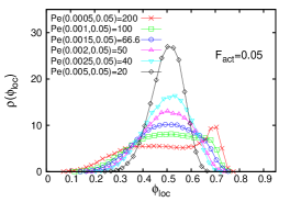
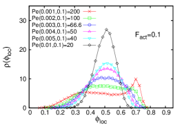
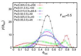
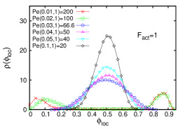
Figure 1: Probability distributions for the local density $\phi_{\rm loc}$ at Péclet numbers given in the keys in the form Pe$(T,F_{\rm act})$ for different temperatures, and $F_{\rm act}=0.05,\ 0.1,\ 0.5,\ 1$ in the different panels. The global density of the system is $\phi=0.5$.

The model has three important energy scales, $\epsilon$, $k_{B}T$ and $F_{\rm act}\sigma_{\rm d}$. There is another energy scale related to the elastic constant $k$ but, since we consider stiff dumbbells in this paper, we do not vary $k$. Keeping also $\epsilon$ and the other parameters listed at the beginning of this section fixed, we will try to determine whether the phase diagram depends upon $k_{B}T$ and $F_{\rm act}\sigma_{\rm d}$ separately or only though their ratio, i.e. through the Péclet number Pe, as usually assumed Redner et al. (2013). The other free parameter to be varied is the global density of the sample, $\phi$.

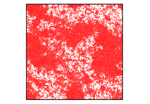
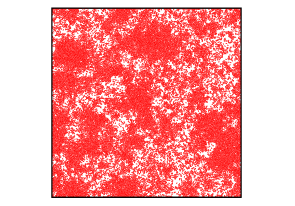
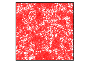
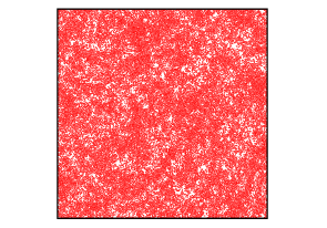
Figure 2: Snapshots of the system for $F_{\rm act}=0.1$ (cfr. the upper right panel in Fig. 1), and $T=0.001,\ 0.002,\ 0.003,\ 0.01$ corresponding to Pe = $200,\ 100$, both phase separated, Pe = $66$, close to critical, and Pe $=20$, homogeneous (from left to right and from top to bottom). The global density is $\phi=0.5$.

In the four panels in Fig. 1 we show the probability distribution function, $\rho$, of the local density, $\phi_{\rm{loc}}$, for four values of the active force, $F_{\rm act}=0.05,\ 0.1,\ 0.5,\ 1$. Each panel contains results for the same set of Péclet numbers Pe$(T,F_{\rm act})$ obtained by different combinations of temperature and active force. The system has global packing fraction $\phi=0.5$. We used the same operative definition of the local density as in Gonnella et al. (2014); Suma et al. (2014a). We divided the full system in square plaquettes with linear size $10\sigma_{\rm d}$ that is much smaller than the linear size of the full sample and big enough to sample $\phi_{\rm{loc}}$ correctly. We improved the statistics by sampling over many different runs of the same kind of system.

At low Pe the system is homogeneous and $\rho$ is peaked around $\phi_{\rm{loc}}=\phi=0.5$. The critical Pe at which the system starts aggregating is approximately the same in all panels, Pe $\simeq 65$. Around this value the density distribution $\rho$ not only becomes asymmetric but starts developing a second peak at $\phi_{\rm{loc}}>0.5$ that characterises the dense phase in the system. Snapshots of typical configurations at $F_{\rm act}=0.1$ and four values of Pe are shown in Fig. 2. The location of the central peak at Pe less than the critical value is independent of all parameters (apart from $\phi$) while the location of the peak at $\phi_{\rm{loc}}>0.5$ is situated at different values of $\phi_{\rm{loc}}$ for different $F_{\rm act}$ and the same Pe (compare the different panels in Fig. 1). The reason for this is that the strength of the interactions between the dumbbells under different $F_{\rm act}$ is different as $F_{\rm act}/\epsilon$ varies with $F_{\rm act}$. A larger active force permits the dumbbells to be more compact, while a lower one favors looser clusters.

We repeated the analysis above for the cases with total packing fractions $\phi=0.3,\ 0.4,\ 0.6$. We found the same values for the densities of the separated phases at $\phi=0.4,\ 0.6$ and Pe = $100,\ 200$, and at $\phi=0.3$ and Pe = 200. At $\phi=0.3$ and $\rm{Pe}\leq 100$ the effects of the presence of the spinodal line require a more elaborate analysis of the phase diagram, as discussed in Suma et al. (2014a). In Table 1 we report these density values for the cases with $F_{\rm act}=1,\ 0.5,\ 0.1,\ 0.05$ and Pe $=100,\ 200$. As observed, the coexistence values get closer for smaller active forces even though the Péclet number remains the same.

Pe	$\ F_{\rm act}=0.05\$	$\ F_{\rm act}=0.1\$	$\ F_{\rm act}=0.5\$	$\ F_{\rm act}=1\$
200	0.37	0.34	0.21	0.049
	0.70	0.71	0.80	0.890
100	0.44	0.41	0.37	0.096
	0.66	0.68	0.77	0.870

Table 1: Density values of the two coexisting phases measured from the histograms in Fig. 1 at $\phi=0.5$. The first and the third lines refer to the dilute phase while the two other lines correspond to the aggregated phase. Similar values are obtained at $\phi=0.4,0.6$ (Pe = $100,\ 200$) and at $\phi=0.3$ (Pe $=200$).

In Fig. 2 we show four snapshots of the system configuration. The active force is $F_{\rm act}=0.1$ in all panels and temperature is increased from left to right and from top to bottom. The configuration in the upper-left panel (Pe = 200) shows phase separation with large scale clusters while the configuration in the lower-right panel (Pe = 20) is clearly homogeneous. The case Pe = 100 is in the segregated phase while the one for Pe = 66 is close to critical.

IV.2 Translational diffusion properties

In Ref. Wu and Libchaber (2000) the diffusion properties of a tracer immersed in a bacterial bath were monitored. A cross-over between a super-diffusive regime at short time-delays and a diffusive regime at long time-delays was reported. The cross-over time was found to increase linearly with the density of the active medium, showing that the cross-over is not due to the tracer’s inertia but to the dynamical properties of the bacterial bath. We explore here the same issues by focusing on the MSD of the center of mass of the dumbbells, defined in Eq. (38). We will consider, for the rest of the paper, sufficiently low Péclet numbers such that the system will always be in the homogenous phase even though fluctuation effects can be relevant, as we will see.

IV.2.1 Dumbbell trajectories

Several single dumbbell trajectories are shown in Fig. 3 for different values of the temperature and global density, under the same active force $F_{\rm act}=0.1$. The trajectories correspond to a total time interval that includes the late diffusive regime (see below). At low temperature and global density ($T=0.005$ and $\phi=0.1$, upper left panel) we see periods of long directional motion. These are reduced at higher global density ($\phi=0.4$ upper right panel). Increasing temperature at $\phi=0.1$ ($T=0.05$ and $T=0.5$ lower left and right panels, respectively) the trajectories become more similar to the typical ones of passive diffusion. While the trajectories are very stretched at $T=0.005$, they become the most compact in the intermediate case at $T=0.05$ and again quite stretched in the last case at $T=0.5$. This behaviour corresponds to the non monotonic behavior of the translational diffusion constant of Eq. (45) in terms of temperature. It decreases going from $T=0.005$ to $T=0.05$ while it increases going from $T=0.05$ to $T=0.5$. The single dumbbell diffusion coefficient, as calculated from Eq. (45),is $D_{A}=0.050,\ 0.0075,\ 0.025$ for the cases at $T=0.005,\ 0.05,\ 0.5$, respectively.

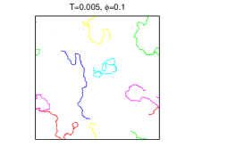
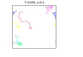
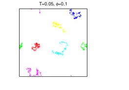
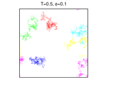
Figure 3: Several trajectories of one bead in different dumbbells. The active force is $F_{\rm act}=0.1$ and the evolution time interval is $t=10000$ in all panels. The other parameters are $T=0.005$ and $\phi=0.1,\ 0.4$ (upper panels, left and right), and $T=0.05,\ 0.5$ and $\phi=0.1$ (lower panels, left and right). The values of the single dumbbell diffusion coefficient, as calculated from Eq. (45), are $D_{A}=0.050,\ 0.0075,\ 0.025$ for the cases at $T=0.005,\ 0.05,\ 0.5$, respectively.

IV.2.2 Four dynamic regimes

In Fig. 4 we show the center of mass MSD normalised by time-delay in such a way that normal diffusion appears as a plateau. The four panels display data at four temperatures, $T=0.005,\ 0.01,$ $0.05,\ 0.1$, all under the same active force $F_{\rm act}=0.1$. Each panel has five curves in it, corresponding to five different densities given in the key. In all cases $m_{\rm d}=1$ and $\gamma=10$ implying $t_{I}=0.1$. The characteristic times $t_{I},\ t^{*},\ t_{a}$ are shown with small vertical arrows in each panel. These plots show several interesting features:
– In all cases there is a first ballistic regime (the dashed segment close to the data is a guide-to-the-eye) with a pre-factor that is independent of $\phi$ and increases with temperature as given by Eq. (39) (The case $t\ll t_{I}$ of the single dumbbell.)

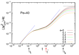
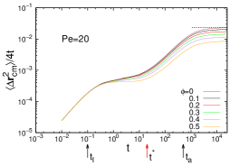
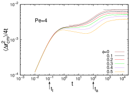
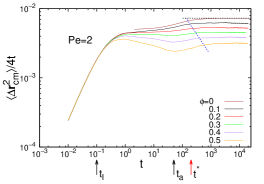
Figure 4: The center of mass MSD normalised by time-delay, for an active system under $F_{\rm act}=0.1$ at $T=0.005,\ 0.01,\ 0.05,\ 0.1$ (Pe = $40,\ 20,\ 4,\ 2$), at the different densities given in the key. The Péclet number decreases from one panel to the other. It induces a strong qualitative change in $\langle\Delta{\mathbf{r}}_{\rm cm}^{2}\rangle$, see the text for a detailed discussion. The two dashes in the first panel represent the ballistic dependence $\simeq t^{2}$. The dashed line in the last panel is a guide-to-the-eye for the density dependence of the last cross-over time-delay that increases weakly with $\phi$. The horizontal dotted lines at long times correspond to the values of the single dumbbell diffusion constant $D_{A}$ from Eq. (45). The vertical black arrows indicate the single dumbbell time-scales $t_{I}$ and $t_{a}$, while the red arrows indicate the single dumbbell characteristic time $t^{*}$, for each case. In the case with $\mbox{Pe}=4$ the times $t^{*}$ and $t_{a}$ coincide. The curves for $\phi=0$ are obtained from Eq. (40), valid in the limit $t\gg t_{I}=0.1$; for this reason they start from the middle of the graph.

– Next, the dynamics slow down and, depending on $T$ and $\phi$, the normalised mean-square displacement may attain a plateau associated to normal diffusion (low $T$) or even decrease, suggesting sub-diffusion. (The case $t_{I}\ll t\ll t^{*}\ll t_{a}$ of the single dumbbell.)
– The dynamics accelerate next, with a second super-diffusive regime in which the curves for all $\phi$ in each panel look approximately parallel and very close to ballistic at $T=0.005,\ 0.01,\ 0.05$. (The case $t_{I}\ll t^{*}\ll t\ll t_{a}$ of the single dumbbell.)
– Finally, the late normal diffusive regime is reached with all curves saturating at a plateau that yields the different $D_{A}$ coefficients. (The case $t_{I}\ll t^{*},\ t_{a}\ll t$ of the single dumbbell.)

It is hard to assert whether the intermediate regime is super-diffusive or simply ballistic as the time-scales $t^{*}$ and $t_{a}$ are not sufficiently well separated (and not even ordered as $t^{*}<t_{a}$ in the last panel). Moreover, in the last two panels (high $T$ or low Pe) the diffusion-ballistic-diffusion regimes are mixed, due to the fact that the condition $t^{*}\ll t_{a}$ is no longer satisfied. The effective slope in the intermediate super-diffusive regime decreases when the density increases.

A rather good fit of the finite density data in the limit Pe $\gg 1$ and for time-delays such that $t\geq t^{*}$ is achieved by using the single dumbbell expression in Eq. (40)

$$\langle\triangle{\mathbf{r}}_{\rm cm}^{2}\rangle(t)=4D_{A}^{\phi}\bigg{(}t-\frac{1-e^{-D_{R}^{\phi}t}}{D_{R}^{\phi}}\bigg{)}\;,$$ (46)

without the first term (negligible if Pe $\gg 1$) and upgrading the remaining parameters, $D_{A}^{\phi}$ and $D_{R}^{\phi}$, to be density-dependent fitting parameters, as done in Wu and Libchaber (2000); Fily and Marchetti (2012). This is shown in Fig. 5 (left panel). For not that large values of Pe one could recover the remaining parameter and use instead $\langle\triangle{\mathbf{r}}_{\rm cm}^{2}\rangle(t)=4D^{{\rm pd},\phi}_{\rm cm}t+4D_{A}^{\phi}(t-\frac{1-e^{-D_{R}^{\phi}t}}{D_{R}^{\phi}})$ with an additional fitting parameter. Figure 5 (right panel) also shows a good agreement between the values of $D_{R}^{\phi}$ found in these fits and the values of the rotation diffusion coefficient $D_{R}(F_{\rm act},T,\phi)$ coming from the late time-delay diffusive regime in the rotational MSD discussed in Sec. IV.3.

The cross-over time-delay between the last ballistic or super-diffusive, and the diffusive regimes seems quite $\phi$-independent in the first two panels $T=0.005,\ 0.01$ and it increases, though rather weakly, with $\phi$, in the last two panels, $T=0.05,\ 0.1$, see the inclined dashed line in the last panel that is also a guide-to-the-eye. This cross-over time-delay is the one that we could associate to the cross-over time between a superdiffusive regime and the last diffusive regime found in the experiment in Wu and Libchaber (2000). The strongest effect of density is though on the first diffusive or sub-diffusive regime.

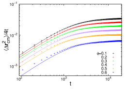
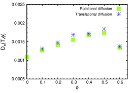
Figure 5: Left panel: Fit of the center of mass MSD normalised by time-delay with the expression in Eq. (46). Pe $=40$ and the different data sets correspond to the global densities given in the key. Right panel: The rotation diffusion coefficient as extracted from the fit of the center–of–mass MSD shown in the left panel ($D_{R}^{\phi}$ in Eq. (46) - blue stars), and from the late-time diffusive rotational MSD directly measured as shown in Sec. IV.3 (green squares). Statistical errors are within the size of the symbols used in the figure.

In summary, no large qualitative change in the center of mass MSD behavior is observed in the range $\phi\in[0,0.6]$. There is just a natural slowing down of the dynamics with larger packing fractions that translates into a change from diffusive to sub-diffusive behavior in the second regime and a general decrease of the diffusion constant in the last regime for all Pe. We study the dependence of the diffusion constant with Pe in detail below.

IV.2.3 The late-epochs translation diffusion coefficient

Let us now discuss the normal diffusive regime at longest time-lags. In Suma et al. (2014b) we studied the translational diffusion coefficient $D_{A}$ as a function of $F_{\rm act}$ and $\phi$ at fixed temperature. In particular, we compared the $\phi$ dependence to the Tokuyama-Oppenheim law for colloids *[][.Inthisworkthediffusioncoefficientforacolloidalsystematfinitedensity$ϕ$isevaluatedas$D(ϕ)/D(0)=(1+H(ϕ))^-1$; with$H(ϕ)$afunctionof$ϕ$withoutfreeparametersreducingtoalineardecreasingofD($ϕ$)atsmall$ϕ$.]Tokuyama. Here, we first examine, instead, the $T$ and $\phi$ dependence of $D_{A}$ for fixed active force, $F_{\rm act}$. Then we consider how the dependence of $D_{A}$ from $T$ and $F_{\rm act}$ can be re-expressed in terms of the Péclet number. The main results for $D_{A}$ obtained in Suma et al. (2014b) will also be revisited in this subsection.

The first question we want to answer is whether $D_{A}$ depends on $k_{B}T$ as for the single dumbbell case ($\phi=0$), the functional form recalled in Eq. (45). For $F_{\rm act}\sigma_{\rm d}/k_{B}T\ll 1$ such that the quadratic term can be neglected this equation implies the linear growth of $D_{A}$ with $k_{B}T$ as in the passive limit. Instead, when the second term dominates, i.e. for very small thermal energy with respect to the work performed by the active force, $D_{A}$ should decay as $1/(k_{B}T)$ with a slope that is quadratic in $F_{\rm act}\sigma_{\rm d}$.

In Fig. 6 we display $D_{A}$ as a function of $T$ for various values of $\phi$ given in the key and $F_{\rm act}=0.1$. The theoretical values for $\phi=0$ are included in the figure (with open triangles joined by a dotted curve). Here, we used the measured value for the distance between the centres of the two colloids, that is $r\approx 0.96\ \sigma_{\rm d}$. In the rest of this section we simply call $\sigma_{\rm d}$ the molecular length and we take $\sigma_{\rm d}=0.96$.

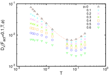
Figure 6: The center of mass diffusion coefficient, $D_{A}$, as a function of temperature, $T$, at different densities $\phi$ given in the key and fixed active force, $F_{\rm act}=0.1$. The triangular data points joined by a dotted curve labeled $\phi=0$ are given by the theoretical $D_{A}$ with $\sigma_{\rm d}=0.96$.

The error-bars are smaller than the symbol size and we do not display them. The curves show a minimum located at $k_{B}T_{\rm min}=F_{\rm act}\sigma_{\rm d}/\sqrt{2}$ for $\phi=0$, that weakly increases with $\phi$. The two regimes, Pe $\ll 1$ and Pe $\gg 1$, still exist and $D_{A}$ is dominated by thermal fluctuations in the former and by the work done by the active force in the latter as in the single dumbbell limit. We see a saturation of $D_{A}$ at small values of $T$ for $\phi>0.2$ and therefore the breakdown of the single dumbbell $1/(k_{B}T)$ behaviour at low temperatures. Instead, at high temperatures $D_{A}$ seems to retain the linear growth with temperature of the single dumbbell at least for the temperatures used in the simulations.

Figure 6 also shows that for the Pe that we used $D_{A}$ is a decreasing function of $\phi$ at all fixed temperatures. This fact can be better appreciated in the left panel in Fig. 7, where $D_{A}$ is plotted as a function of $\phi$ for various temperatures given in the key. (Recall that the $\phi$ dependence of $D_{A}$ at fixed $T$ and for different active forces was discussed in Suma et al. (2014b) where it was shown how the Tokuyama-Oppenheim Tokuyama and Oppenheim (1994) law of the passive system was simplified under activation to a decay that is close to a simple exponential. We will come back to this issue below.)

The non-monotonicity of $D_{A}$ as a function of $T$ already discussed in Fig. 6 is confirmed by the data presentation in Fig. 7, with the minimum situated around $T\simeq 0.07$. In the right panel we observe the opposite behaviour in the ratio $D_{A}(F_{\rm act}=0.1,T,\phi)/D_{A}(F_{\rm act}=0.1,T,0)$, first growing for increasing $T$ to reverse its trend at around $T\simeq 0.05-0.07$. Consistently with the behaviour found in Suma et al. (2014b), there are temperatures such that the data for the above ratio cross each other when the density is increased, see for example $T=0.01,\ 0.1$ (or Pe $=2,\ 20$). The right panel in Fig. 7 also shows that a very small density can have relevant effects on the behaviour of the diffusion coefficient.

We have repeated this analysis for a stronger active force and we found that the results are consistent, with a cross-over temperature that grows with $F_{\rm act}\sigma_{\rm d}$, as predicted by the single dumbbell equation, though we cannot assert that the dependence be linear.

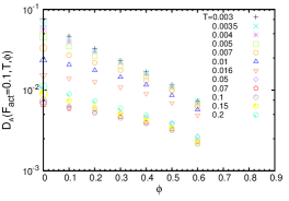
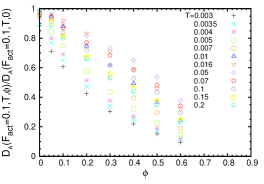
Figure 7: Center of mass diffusion constant at various $T$ given in the key (left panel) and center of mass diffusion constant over the one for one dumbbell (right panel) both as a function of $\phi$. The smallest densities considered are $\phi=0$ in the left panel and $\phi=0.001$ in the right panel. The active force is fixed to $F_{\rm act}=0.1$. The symbol convention is the same in the two panels.

Next, we analyse in Fig. 8 whether the ratio of diffusion coefficients of the active system at finite density and single passive dumbbell $D_{A}(F_{\rm act},T,\phi)/D_{\rm cm}^{\rm pd}$ depends only on the Péclet number, as it does for the single dumbbell problem. With this aim, we fix $F_{\rm act}$ and we vary $T$, and the values Pe = $4,\ 20,\ 40,\ 66$ in each panel are obtained from three different combinations of $F_{\rm act}$ and $T$. In all panels the collapse of data is very good. Note the change in concavity of the collapsed data that occurs at Pe = 20. This value is relatively far from the transition between homogeneous and segregated phases estimated in Suma et al. (2014a, b), and the system configurations are still homogeneous, see the last panel in Fig. 2, though with a distribution of local densities, $\phi_{\rm{loc}}$, with a certain width, see Fig. 1.

These results suggest

$$D_{A}(F_{\rm act},T,\phi)=k_{B}T\ f_{A}\left(\mbox{Pe},\phi\right)$$ (47)

with $f_{A}(\mbox{Pe},0)=(2\gamma)^{-1}(1+\mbox{Pe}^{2}/8)=D_{A}(F_{\rm act},T,0)/(k_{B}T)$ and $f_{A}$ a decreasing non-linear function of $\phi$ at fixed Pe. This relation is equivalent to

$$\frac{D_{A}(F_{\rm act},T,\phi)}{D_{A}(F_{\rm act},T,0)}=\frac{f_{A}(\mbox{Pe},\phi)}{f_{A}(\mbox{Pe},0)}\;.$$ (48)

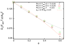
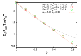
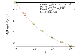
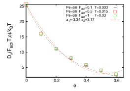
Figure 8: Center of mass diffusion constant, $D_{A}$, over $k_{B}T$ for Pe $=4,\ 20,\ 40,\ 66$ as shown in the keys. For each value of the Péclet number three couples of values of $F_{\rm act}$ and $T$ were used. The black dotted lines are exponential fits to the data points, as suggested by Eq. (50). The red line-points are the quadratic fit in Eq. (51) with fitting parameters given in the keys. See the text for a discussion.

The l.h.s. is what we studied in Suma et al. (2014b) as a function of $F_{\rm act}$ and $\phi$, keeping $T$ fixed, and we proposed

$$\frac{D_{A}(F_{\rm act},T,\phi)}{D_{A}(F_{\rm act},T,0)}=e^{-b(F_{\rm act})\phi}$$ (49)

with $b$ a non-monotonic fitting function of $F_{\rm act}$. Knowing now that $D_{A}/(k_{B}T)$ depends on $F_{\rm act}$ and $T$ only through Pe, we deduce

$$D_{A}(F_{\rm act},T,\phi)=D_{\rm cm}^{\rm pd}\ (1+\mbox{Pe}^{2}/8)\ e^{-b({\rm Pe})\phi}\;.$$ (50)

Note that in Suma et al. (2014b) the maximum in $b$ appeared at $F_{\rm act}\simeq 0.1$ that, for the temperature used, $T=0.05$, corresponds to Pe $\simeq 4$. Thus, $f_{A}(\mbox{Pe},\phi)$ should be monotonically increasing with Pe, at all fixed $\phi$, as it results when comparing the data on the different panels in Fig. 8. In Fig. 8 we included, with dotted black lines, the exponential fits in Eq. (50) where the only free parameter is $b(\mbox{Pe})$. The values of $b(\mbox{Pe})$ are $1.1,\ 1.6,\ 2.8,\ 4.1$ for Pe = $4,\ 20,\ 40,\ 66$, in agreement with what we reported in Suma et al. (2014b).

However, while we see that the exponential fit is very good at all $\phi$ for Pe = $40$ and Pe = $66$, it is not as good for the smaller Pe data. The red line-points in Fig. 8 represent, instead, the result of the fit

$$D_{A}(F_{\rm act},T,\phi) = D_{A}(F_{\rm act},T,0)$$ (51)

$$\times[1+a_{1}(\mbox{Pe})\ \phi+a_{2}(\mbox{Pe})\ \phi^{2}]\;.$$

This functional form gives a better representation of the data than the exponential for Pe = $4$ and Pe = $20$, which is, in a sense, natural since one expects to recover a rather complex Tokuyama-Oppenheim like form in the limit Pe $\to 0$. The exponential and polynomial fits are of equivalent quality for Pe = $40$, while the polynomial fit is clearly worse than the exponential one for Pe = $66$. The fitting parameters are given in the keys. One notices that $a_{1}$ is negative in all cases while $a_{2}$ changes sign from negative at Pe $<20$ to positive at Pe $>20$ (leading to a growing behaviour at large $\phi$ that is not physical). At Pe = 20 the density dependence is almost linear as $a_{2}$ is very close to zero.

IV.3 Rotational diffusion properties

Having discussed in detail the translational diffusion properties we turn now to the rotational ones.

IV.3.1 Dynamic regimes

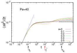
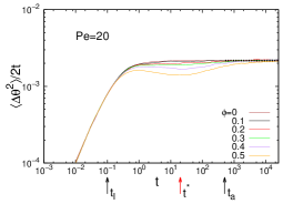
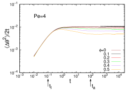
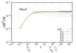
Figure 9: The angular MSD for the Pe numbers in the labels and, with different lines, various densities given in the keys to each panel. The dash in the first panel highlights the initial ballistic behavior. The vertical arrows indicate the characteristic times $t_{I},\ t^{*},\ t_{a}$. The horizontal dotted lines at long times correspond to the values of the single dumbbell diffusion constant $D_{R}$ from Eq. (32). Note that the vertical scale is different in the two panels above and in the two panels below.

In Fig. 9 we display the angular MSD normalized by time-delay. The four panels show data obtained for the same parameters as the ones used in Fig. 4 with $F_{\rm act}=0.1$. Each panel, corresponding to the cases with $T=0.005,\ 0.01,\ 0.05,\ 1$ (Pe = $40,\ 20,\ 4,\ 2$, respectively), includes curves for five finite densities, $\phi=0.1,\ 0.2,\ 0.3,\ 0.4,\ 0.5$, and the single dumbbell limit, $\phi=0$, as labeled in the key. These plots also show several interesting features:

– In all cases there is a first ballistic regime with a pre-factor that is independent of $\phi$ and increases with temperature (The case $t\ll t_{I}=m_{\rm d}/\gamma$ of the single dumbbell.)
– Next, the dynamics slow down and, depending on $T$ and $\phi$, the normalised MSD may attain an ever-lasting plateau associated to normal diffusion for low $\phi$ at any temperature, or even decrease, suggesting sub-diffusion, at high enough $\phi$.
– At low temperature $T=0.005,\ 0.01$ (Pe = $40,\ 20$) and sufficiently high density the dynamics accelerate next, with a second super-diffusive regime that crosses over to a final diffusive regime.
– In the late normal diffusive regime all curves saturate and the height of the plateau yields the different $D_{R}$ coefficients that we discuss below.

The effect of Pe and $\phi$ are stronger on the rotational MSD than on the translational MSD. New regimes appear in the rotational collective motion with respect to the individual molecular limit. In the phase separated regime the dumbbell clusters rotate Gonnella et al. (2014); Suma et al. (2014a). It is possible that strong fluctuations not far from the critical point (Pe = 20, 40) have an important rotational component than enhances/advects rotational diffusion giving rise to an observable contribution to displacement also manifestating itself in the appearing of new dynamical regimes.

IV.3.2 The late-epochs rotation diffusion coefficient

We now study whether the linear temperature dependence of the single dumbbell angular diffusion constant, Eq. (32), survives the interactions between dumbbells in the finite density problem, see Fig. 10. The data points are compatible with a linear behaviour at sufficiently high temperature, with a slope that depends upon $\phi$. The trend in the curves reverses below the cross-over at $T\simeq 0.01$ with larger values of $D_{R}$ for larger values of $\phi$ (see the right panel in the same figure).

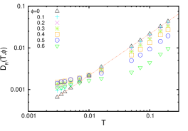
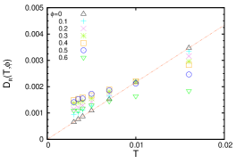
Figure 10: Angular diffusion constant as a function of $T$, for $F_{\rm act}=0.1$ at fixed $\phi$ in logarithmic scale (left panel) and a zoom on the low temperature behaviour in linear scale (right panel). The data points joined with a line for $\phi=0$ represent the theoretical expectation (32).

From Fig. 11 one easily concludes that the $F_{\rm act}$-independence of $D_{R}$ is lost as soon as the interaction between dumbbells is switched on at finite density. This fact can be seen, for instance, by comparing the $T=0.1$ data, one of the two temperatures included in both panels, sharing the same value, slightly larger than $10^{-2}$, at $\phi=0$. While in the case $F_{\rm act}=0.1$ (left panel) $D_{R}$ clearly decreases with $\phi$, in the case $F_{\rm act}=1$ (right panel) $D_{R}$ is almost constant. These figures also show the change in trend operated at an $F_{\rm act}$-dependent $T$: at high temperature $D_{R}$ decreases with $\phi$ while at low temperature $D_{R}$ increases with $\phi$. The change occurs at $T\simeq 0.01$ for $F_{\rm act}=0.1$ and at $T\simeq 0.1$ for $F_{\rm act}=1$ suggesting that the change is controlled by Pe.

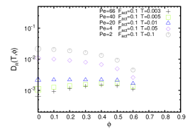
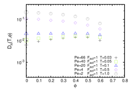
Figure 11: Angular diffusion constant for various $T$ under the same active force $F_{\rm act}=0.1$ (left panel) and $F_{\rm act}=1$ (right panel). The only common temperatures on the two panels are $T=0.05,\ 0.1$ and, consistently, $D_{R}$ at these temperatures is the same at $\phi=0$.

Finally, we analyse whether $D_{R}/(k_{B}T)$ depends on $F_{\rm act}$ only via Pe. To this end, in Fig. 12 we repeat the analysis shown in Fig. 8 for $D_{A}$. The four panels show $D_{R}/(k_{B}T)$ against $\phi$ for Pe = $4,\ 20,\ 40,\ 66$. In each panel we include data for three pairs of $F_{\rm act}$ and $T$ leading to the same Pe. We see that the data points collapse on different master curves in each panel. This suggests

$$D_{R}(F_{\rm act},T,\phi)=k_{B}T\ f_{R}(\mbox{Pe},\phi)$$ (52)

with $f_{R}(\mbox{Pe},0)=f_{R}(0,0)=2/(\gamma\sigma_{\rm d}^{2})$. The data also show a change in trend of the function $f_{R}$ at around Pe = 20. At low densities, while the master curve decreases with $\phi$ for Pe $<20$, it becomes flat at Pe $=20$ and it increases with $\phi$ for Pe $>20$. This would suggest:

$$f_{R}(\mbox{Pe},\phi)\simeq\frac{2}{\gamma\sigma_{\rm d}^{2}}+a(\mbox{Pe},\phi)\ ,$$ (53)

with $a($Pe, $\phi)$ almost linear in $\phi$ and the slope changing sign at Pe $\simeq 20$ for small $\phi$. All panels, i.e. at all Pe, show a cross-over at high enough densities after which the rotational diffusion constant decreases with increasing density.

A possible explanation of the different density-dependence of $D_{R}$ at small and large Péclet can be found from following the evolution of a single tracer dumbbell at intermediate densities, $\phi\approx 0.4$ for example, as it can be seen in the supplementary movies in Ref. . One observes that at low Pe (Pe = 2) the system is very uniformly distributed and the movement of the tracer dumbbell is inhibited by the ‘cages’ formed by surrounding dumbbells. Collisions are frequent but each of them only produces a small angular displacement. In this case the effect of increasing the density is to decrease both the rotational and translational diffusion coefficients. On the other hand, at high Peclet (Pe = 40), small fluctuating clusters can be observed (their presence is also signalled by a peak in the structure factor Suma et al. (2014b)). This has relevant effects on the behaviour of the tracer dumbbell. First, there are particle depleted regions which are large enough to allow significant angular displacements without collisions. Second, angular displacements appear to be enhanced when the tracer dumbbell meets a cluster and is advected by its motion. On the other hand, at still higher densities the cage effect becomes again preeminent so that rotations are inhibited and $D_{R}$ decreases. Note that both $D_{R}$ and $D_{A}$ change behavior at Pe $=20$ (the translational diffusion coefficient $D_{A}$ is a convex function of density for Pe $<$ 20 and changes curvature for Pe $>$ 20). We find the fact that these cross-overs occur at the same Péclet worth to be stressed even though it is difficult to argue about its implications.

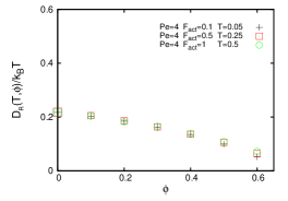
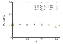
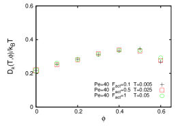
Figure 12: Rotational diffusion constant over $k_{B}T$ for Pe $=4,\ 20,\ 40,\ 66$ as shown in the keys. For each value of the Péclet number three couples of values of $F_{\rm act}$ and $T$ were used. All master curves take the value $2/(\gamma\sigma_{\rm d}^{2})\approx 0.215$ at $\phi=0$. At small $\phi$, there is a noticeable change in trend at Pe $\simeq 20$. At sufficiently large $\phi$ all curves decrease with increasing $\phi$.

V Conclusions

We presented a thorough study of the translational and rotational MSD of a system of interacting active dumbbells. We focused on the regimes where the global system is homogeneous. Higher densities than the ones used in Wu and Libchaber (2000); Leptos et al. (2009) have been considered with the Péclet number small enough (possibly much smaller than in the experiments) to keep the system in the homogenous phase.

We first analysed the single molecule dynamics as a benchmark to later characterize the finite density effects. In the passive case, Pe = 0, the translational and rotational MSDs show a standard cross-over from ballistic motion to normal diffusion at the inertial time $t_{I}=m_{\rm d}/\gamma$. Under the active force, the normal diffusion of the center of mass is accelerated after a time-scale $t^{*}\propto t_{a}/{\mbox{Pe}}^{2}$ with $t_{a}=\gamma\sigma_{\rm d}^{2}/(2k_{B}T)$ and, still later, after $t_{a}$, a new diffusive regime is reached with a diffusion constant that is enhanced with respect to the one in the passive limit as a quadratic function of the Péclet number. Instead, the rotational properties of the active dumbbell are not modified by the longitudinal active force; all torque is exerted by the thermal noise.

Then we turned to the analysis of the mixed density and active force effects on the collective motion of the interacting system.

The rich dynamic structure of the center of mass translational motion of the single molecule, with the four distinct time regimes summarized above, survives under finite densities with modified parameters. The super-diffusive behaviour shown in Wu and Libchaber (2000) is reminiscent of the second ballistic regime in the interacting active dumbbell system at finite densities. The diffusion constant $D_{A}$ in the last diffusive regime has a non-monotonic dependence on temperature, as for the single dumbbell case, and it decreases with increasing self-propelled particle density at all temperatures. Moreover, the ratio $D_{A}/(k_{B}T)$ depends on temperature and active force only through the Péclet number at all densities explored. This ratio, at fixed density, is an increasing function of $\rm Pe$. All these results are consistent with those found in our previous paper Suma et al. (2014b) where it was also shown that the ratio between the translational coefficient diffusion at finite density and the one for the single dumbbell had a non-monotonic Pe dependence.

Next we moved to the analysis of the rotational MSD. While in the single dumbbell case its time-delay dependence is rather simple, with a single cross-over between ballistic and diffusive behaviour, intermediate regimes, roughly for $t_{I}\ll t\ll t^{*}$ and $t^{*}\ll t\ll t_{a}$, appear at finite densities. The late epochs diffusion constant $D_{R}$ increases with temperature (though not linearly) at all densities and active forces simulated. The independence on active force is lost at finite densities. The ratio $D_{R}/(k_{B}T)$ depends on temperature and activity only through the Péclet number. At low densities, its dependence on density changes from decreasing at low Pe to increasing at high Pe. This change in behaviour can be related to the large scale density fluctuations that appear close to the transition from the homogeneous to the aggregated phase at a critical Pe. In the aggregated phase large and rather compact clusters rotate coherently Gonnella et al. (2014); Suma et al. (2014a). Not far from the transition, in the homogenoues phase, fluctuating clusters with some coherent rotation are observable and these may be the cause for the increase of $D_{R}$ with $\phi$. On the other hand, at large enough densities rotations are strongly inhibited and the value of $D_{R}$ decreases for all Pe.

The fluctuations of translational and rotational displacements have been characterized in Cugliandolo et al. (2015). Special emphasis was put on the identification of the regimes in which the fluctuations are non-Gaussian. See this reference for more details.

After this work we plan to analyse the motion of tracers in contact with this active sample and, especially, to analyse the existence of a parameter to be interpreted as an effective temperature from the mobility and diffusive properties of the sample and the tracers, in the manner done in Loi et al. (2008, 2011a, 2011b); Palacci et al. (2010); Shen and Wolynes (2004, 2005); Wang and Wolynes (2011a, b); Tailleur and Cates (2009); Szamel (2014) for different active systems.

Acknowledgments: L. F. C. is a member of Institut Universitaire de France and acknowledges CNRS PICS06691 for financial support. G.G. acknowledges the support of MIUR (project PRIN 2012NNRKAF).

References

- Toner et al. (2005) J. Toner, Y. Tu, and S. Ramaswamy, Ann. of Phys. 318, 170 (2005).
- Fletcher and Geissler (2009) D. A. Fletcher and P. L. Geissler, Ann. Rev. Phys. Chem. 60, 469 (2009).
- Menon (2010) G. Menon, in Rheology of Complex Fluids, edited by J. Krishnan, A. Deshpande, and P. Kumar (Springer, 2010).
- Ramaswamy (2010) S. Ramaswamy, Ann. Rev. Cond. Matt. Phys. 1, 323 (2010).
- Cates (2012) M. E. Cates, Rep. Prog. Phys. 75, 042601 (2012).
- Romanczuk et al. (2012) P. Romanczuk, M. Bär, W. Ebeling, B. Lindner, and L. Schimansky-Geier, Eur. Phys. J. Special topics 202, 1 (2012).
- Vicsek and Zafeiris (2012) T. Vicsek and A. Zafeiris, Phys. Rep. 517, 71 (2012).
- Marchetti et al. (2013) M. C. Marchetti, J. F. Joanny, S. Ramaswamy, T. B. Liverpool, J. Prost, M. Rao, and R. A. Simha, Rev. Mod. Phys. 85, 1143 (2013).
- de Magistris and Marenduzzo (2015) G. de Magistris and D. Marenduzzo, Physica A 418, 65 (2015).
- Gonnella et al. (2015) G. Gonnella, D. Marenduzzo, A. Suma, and A. Tiribocchi, arXiv preprint arXiv:1502.02229 (2015), to be published in ”Comptes Rendus de Physique”.
- Walther and Müller (2013) A. Walther and A. H. Müller, Chem. Rev. 113, 5194 (2013).
- Mendelson et al. (1999) N. Mendelson, A. Bourque, K. Wilkening, K. Anderson, and J. Watkins, J. Bacteriol. 181, 600 (1999).
- Wu and Libchaber (2000) X.-L. Wu and A. Libchaber, Phys. Rev. Lett. 84, 3017 (2000).
- Dombrowski et al. (2004) C. Dombrowski, L. Cisneros, S. Chatkaew, R. Goldstein, and J. Kessler, Phys. Rev. Lett. 93, 098103 (2004).
- Hernández-Ortíz et al. (2005) J. P. Hernández-Ortíz, C. G. Stoltz, and M. D. Graham, Phys. Rev. Lett. 95, 204501 (2005).
- Riedel et al. (2005) I. Riedel, K. Kruse, and J. Howard, Science 309, 300 (2005).
- Sokolov et al. (2007) A. Sokolov, I. Aranson, J. Kessler, and R. Goldstein, Phys. Rev. Lett. 98, 158102 (2007).
- Zhang et al. (2009) H. Zhang, A. Be’er, R. Smith, E.-L. Florin, and H. Swinney, Europhys. Lett. 87, 48011 (2009).
- Tailleur and Cates (2008) J. Tailleur and M. E. Cates, Phys. Rev. Lett. 100, 218103 (2008).
- Fily and Marchetti (2012) Y. Fily and M. C. Marchetti, Phys. Rev. Lett. 108, 235702 (2012).
- Fily et al. (2014) Y. Fily, S. Henkes, and M. C. Marchetti, Soft Matter 10, 2132 (2014).
- Redner et al. (2013) G. S. Redner, M. F. Hagan, and A. Baskaran, Phys. Rev. Lett. 110, 055701 (2013).
- Stenhammar et al. (2013) J. Stenhammar, A. Tiribocchi, R. J. Allen, D. Marenduzzo, and M. E. Cates, Phys. Rev. Lett. 111, 145702 (2013).
- Gonnella et al. (2014) G. Gonnella, A. Lamura, and A. Suma, Int. J. Mod. Phys. C 25, 1441004 (2014).
- Suma et al. (2014a) A. Suma, D. Marenduzzo, G. Gonnella, and E. Orlandini, EPL 108, 56004 (2014a).
- Levis and Berthier (2014) D. Levis and L. Berthier, Phys. Rev. E 89, 062301 (2014).
- Wittkowski et al. (2014) R. Wittkowski, A. Tiribocchi, J. Stenhammar, R. Allen, D. Marenduzzo, and M. Cates, Nat. Comm. 5, 4351 (2014).
- Buttinoni et al. (2013) I. Buttinoni, J. Bialké, F. Kümmel, H. Löwen, C. Bechinger, and T. Speck, Phys. Rev. Lett. 110, 238301 (2013).
- Palacci et al. (2010) J. Palacci, C. Cottin-Bizonne, C. Ybert, and L. Bocquet, Phys. Rev. Lett. 105, 088304 (2010).
- Leptos et al. (2009) K. C. Leptos, J. Guasto, J. Gollub, A. I. Pesci, and R. Goldstein, Phys. Rev. Lett. 103, 198103 (2009).
- Kurtuldu et al. (2011) H. Kurtuldu, J. Guasto, K. Johnson, and J. Gollub, Proc. Nat. Acad. Sc. 108, 10391 (2011).
- Kasyap et al. (2014) T. Kasyap, D. Koch, and M. Wu, Phys. of Fluids 26, 081901 (2014).
- Pushkin and Yeomans (2014) D. Pushkin and J. Yeomans, J. Stat. Mech. , P04030 (2014).
- Morozov and Marenduzzo (2014) A. Morozov and D. Marenduzzo, Soft Matter 10, 2748 (2014).
- Miño et al. (2011) G. Miño, T. E. Mallouk, T. Darnige, M. Hoyos, J. Dauchet, J. Dunstan, R. Soto, Y. Wang, A. Rousselet, and E. Clement, Phys. Rev. Lett. 106, 048102 (2011).
- Llopis and Pagonabarraga (2006) I. Llopis and I. Pagonabarraga, EPL 999, 75 (2006).
- Grégoire and Chaté (2001) G. Grégoire and Y. Chaté, H. Tu, Phys. Rev. E 64, 011902 (2001).
- Valeriani et al. (2011) C. Valeriani, M. Li, J. Novosel, J. Arlt, and D. Marenduzzo, Soft Matter 7, 5228 (2011).
- Suma et al. (2014b) A. Suma, G. Gonnella, G. Laghezza, A. Lamura, A. Mossa, and L. F. Cugliandolo, Phys. Rev. E 90, 052130 (2014b).
- Cugliandolo (2011) L. F. Cugliandolo, J. Phys. A: Math. and Theor. 44, 483001 (2011).
- Weeks et al. (1971) J. D. Weeks, D. Chandler, and H. C. Andersen, J. Chem. Phys. 54, 5237 (1971).
- Note (1) In a system with momentum conservation the total force on a neutrally buoyant swimmer should indeed be zero. However Brownian dynamics theories and simulations neglect fluid-mediated interactions so the only way to propel a particle is to apply a force along its direction.
- Baskaran and Marchetti (2010) A. Baskaran and M. C. Marchetti, J. Stat. Mec. , P04019 (2010).
- Øksendhal (2000) B. Øksendhal, Stochastic differential equations (Springer-Verlag, Berlin, 2000).
- Note (2) The use of Stratonovich calculation is quite natural in this context, as stressed by van Kampen and others Van Kampen (1981), as for most of physical problems. We can also observe that, following the Ito approach Gardiner (1996), the equations of motion for the polar coordinates can be written, neglecting the inertial contribution, as , with , Gaussian white noises satisfying the same properties as , of Eq. (15). This set of equations give the same dynamical equations for the momenta Eqs. (27-29) resulting from Stratonovich approach.
- Gardiner (1996) C. W. Gardiner, Handbook of stochastic methods for physics, chemistry and the natural sciences (Springer-Verlag, Berlin Heidelberg, 1996).
- Coffey et al. (2012) W. T. Coffey, Y. P. Kalmykov, and J. T. Waldron, The Langevin equation - 3rd edition, World Scientific series in contemporary chemical physics, Vol. 27 (World Scientific, Singapore, 2012).
- Note (3) Equation (27) with the l.h.s. set to zero and the potential parameters that we use in the simulations yields quite independently of temperature in the range . In the simulations we find that the fluctuations around this value increase weakly with increasing temperature.
- ten Hagen et al. (2011) B. ten Hagen, S. van Teeffelen, and H. Löwen, J. Phys.: Condens. Matter 23, 194119 (2011).
- Tokuyama and Oppenheim (1994) M. Tokuyama and I. Oppenheim, Phys. Rev. E 50, 16 (1994).
- Note (4) See the supplemental movies 1-6 at [URL will be inserted by publisher]. Movies 1-3 refer to the case Pe = 2 (, ) and increasing densities in order. Movies 4-6 refer to the case of Pe = 40 (, ) and same increasing densities . A tracer dumbbell is coloured in blue to better follow the trajectory of a single particle.
- Cugliandolo et al. (2015) L. F. Cugliandolo, G. Gonnella, and A. Suma, Chaos and solitons - to appear, arXiv:1504.03549 (2015).
- Loi et al. (2008) D. Loi, S. Mossa, and L. F. Cugliandolo, Phys. Rev. E 77, 051111 (2008).
- Loi et al. (2011a) D. Loi, S. Mossa, and L. F. Cugliandolo, Soft Matter 7, 3726 (2011a).
- Loi et al. (2011b) D. Loi, S. Mossa, and L. F. Cugliandolo, Soft Matter 7, 10193 (2011b).
- Shen and Wolynes (2004) T. Shen and P. G. Wolynes, Proc. Nac. Acad. Sc. USA 101, 8547 (2004).
- Shen and Wolynes (2005) T. Shen and P. G. Wolynes, Phys. Rev. E 72, 041927 (2005).
- Wang and Wolynes (2011a) S. Wang and P. G. Wolynes, J. Chem. Phys. 135, 051101 (2011a).
- Wang and Wolynes (2011b) S. Wang and P. G. Wolynes, Proc. Nac. Acad. Sc. 108, 15184 (2011b).
- Tailleur and Cates (2009) J. Tailleur and M. E. Cates, EPL 86, 60002 (2009).
- Szamel (2014) G. Szamel, Phys. Rev. E 90, 012111 (2014).
- Van Kampen (1981) N. Van Kampen, Journal of Statistical Physics 24, 175 (1981).