Leading-order hadronic contributions to the electron and tau anomalous magnetic moments

Abstract

The leading hadronic contributions to the anomalous magnetic moments of the electron and the $\tau$-lepton are determined by a four-flavour lattice QCD computation with twisted mass fermions. The results presented are based on the quark-connected contribution to the hadronic vacuum polarization function. The continuum limit is taken and systematic uncertainties are quantified. Full agreement with results obtained by phenomenological analyses is found.

1 Introduction

The standard model of particle physics (SM) contains three charged leptons $l$, mainly differing in mass, the electron, the muon, and the $\tau$-lepton with $m_{e}:m_{\mu}:m_{\tau}\approx 1:207:3477$ Agashe:2014kda . Their magnetic moments, in particular their so-called anomalous magnetic moments, $a_{l}=(g-2)_{l}/2$, control their behaviour in an external magnetic field.

Being the lepton with the smallest mass, the electron is stable. This leads to the electron magnetic moment being one of the most precisely determined quantities in nature. The difference between the latest experimental Hanneke:2008tm and SM values Aoyama:2012wk ; Aoyama:2014sxa is of $\mathcal{O}\left(10^{-12}\right)$ or approximately 1.3 standard deviations, c.f. Giudice:2012ms and references therein,

$$a_{e}^{\mathrm{Exp}} = 115\,965\,218\,07.3\,(2.8)\times 10^{−13}$$

$$a_{e}^{\mathrm{SM}} = 115\,965\,218\,17.8\,(7.6)\times 10^{-13}$$

$$a_{e}^{\mathrm{Exp}}-a_{e}^{\mathrm{SM}} = -10.5\,(8.1)\times 10^{-13}\,.$$

This constitutes one of the cornerstone results for quantum field theories to be recognised as the correct mechanism for describing particle interactions. The very good agreement of the electron magnetic moment between experiment and SM calculations is not matched by the muon anomalous magnetic moment. In fact, here a two to four sigma discrepancy is observed, see e.g. Brambilla:2014jmp . One reason for the observed discrepancy could be that the magnetic moment of the muon receives larger non - perturbative contributions than the one of the electron. On the other hand, it is supposed to be also more sensitive to beyond the SM physics, since for a large class of theories new physics contributions are expected to be proportional to the squared lepton mass. Thus it is a prime candidate for detecting physics beyond the SM. Due to the large mass of the $\tau$-lepton, it would be the optimal lepton for finding new physics. However, because its lifetime is very short ($\mathcal{O}\left(10^{-13}\right)$s) there currently only exist bounds on its anomalous magnetic moment from indirect measurements Abdallah:2003xd .

The QED Aoyama:2012wj ; Aoyama:2012wk and the electroweak contributions Czarnecki:1995wq ; Czarnecki:1995sz to the lepton anomalous magnetic moments have been computed in perturbation theory to impressive five and two loops, respectively. The main uncertainties remaining in the theoretical determinations of the anomalous magnetic moments originate thus from the leading-order (LO) hadronic contributions. Since they are particularly sensitive to those virtual photon momenta that are of $\mathcal{O}\left(m_{l}^{2}\right)$, these contributions are inherently non-perturbative and not accessible to perturbation theory. In order to have a prediction of the anomalous magnetic moments from the SM alone, a non-perturbative method needs to be employed and the only such approach we presently know, which eventually allows us to control all systematic uncertainties, is lattice QCD (LQCD) which we use here.

As highlighted in Giudice:2012ms , the uncertainty in the comparison between the experimental and the SM value for the electron anomalous magnetic moment is currently dominated by the experimental uncertainty of its determination and the value for $\alpha_{\rm QED}$ from atomic physics experiments with rubidium atoms which both are to be reduced in the future. Recently, the Harvard group has announced to be working on a more accurate determination of the electron as well as the positron $(g-2)$ Hoogerheide:2014mna . According to Ref. Giudice:2012ms , uncertainties in the sub-$10^{-13}$ region might be expected which would clearly provide the opportunity to also detect new physics contributions in the anomalous magnetic moment of the electron and thus to cross-check the muon discrepancy. In this situation it will again be of utmost importance to know the hadronic contributions as precisely as possible.

Furthermore, even for the $\tau$-lepton, Ref. Pich:2013lsa lists several proposals for the first actual measurement of its anomalous magnetic moment, e.g. Fael:2013ij . A first successful measurement in this direction has been reported in Oberhof:2015hea . As we will show in the following, compared to the case of the muon it will be much easier to obtain a value for the LO QCD contribution to $a_{\tau}$ from LQCD with the required precision to detect new physics and it will probably not take very long before the QCD contribution entering the official SM result will be provided by LQCD.

As mentioned before, the hadronic LO contributions to the anomalous magnetic moments of the three SM leptons, $a_{l}^{\rm hvp}$, strongly depend on the values of their masses. Since the magnitude of the lepton masses spans four orders of magnitude, the corresponding contributions to the anomalous magnetic moments differ substantially and probe very different energy regions, see also the discussion of Fig. 1 in Sect. 3.

In this article, we present the results of our four-flavour computations of the quark-connected, LO hadronic vacuum polarisation contributions to the electron and $\tau$-lepton anomalous magnetic moments obtained from the (maximally) twisted mass formulation of LQCD. The muon case has already been covered in Burger:2013jya . The important feature of the present calculation is that we adopt exactly the same strategy as for the muon Burger:2013jya including the same chiral and continuum extrapolations. Thus, the results presented here are not only interesting in themselves, but also serve as an important cross-check for our treatment of the hadronic vacuum polarisation function. The consistent picture we obtain for all three standard model leptons then reassures the validity of the analysis approach.

Additionally to the systematic uncertainties investigated in our previous paper, we quantify the light-quark disconnected contributions on one of our $N_{f}=2+1+1$ ensembles in order to arrive at a rough estimate of their systematic effect on our estimates for the hadronic LO anomalous magnetic moments. A full quantitative constraint on the quark-disconnected contribution, however, is beyond the scope of this work.

Another very important feature is that incorporating the complete first two generations of quarks enables us to directly and unambiguously compare our results with the values obtained from phenomenological analyses relying on experimental data and a dispersion relation. We note that the contributions from third-generation quarks can be neglected, since they are smaller than the current theoretical accuracy, as can be inferred e.g. from the data tables of Ref. Benayoun:2012wc . Recently, the bottom quark contribution to $a_{\mu}^{\rm hvp}$ has been explicitly computed on the lattice Colquhoun:2014ica confirming it to be one order of magnitude smaller than the current uncertainty of the phenomenological determinations of $a_{\mu}^{\rm hvp}$.

Additionally to the $N_{f}=2+1+1$ flavour ensembles Baron:2010bv ; Baron:2010th at unphysically large pion masses studied in Burger:2013jya , we computed the dominant light quark contributions to the anomalous magnetic moments on a $N_{f}=2$ flavour ensemble directly at the physical point Abdel-Rehim:2013yaa ; Abdel-Rehim:2014nka . This allows us to test the chiral extrapolations performed when using the reparametrisation introduced in Feng:2011zk ; Renner:2012fa . Since we currently only have one ensemble at the physical point with one lattice spacing and we neglect the small influence of the strange and charm sea quarks when comparing the results from $N_{f}=2$ and $N_{f}=2+1+1$ ensembles, a final conclusion is precluded at this point. The significance of this comparison is based on the empirically observed weak dependence on the lattice spacing of the light quark contribution as well as the marginal sea quark effects from strange and charm on the latter.

The next section comprises a short repetition of the most important equations needed to follow the discussion of the results for the LO hadronic vacuum polarisation contributions to the anomalous magnetic moments of the electron in Sect. 3 and the $\tau$-lepton in Sect. 4. In Sect. 5 we summarise our results and draw our conclusions.

2 Computation of $a_{l}^{\rm hvp}$

The LO hadronic contribution to the lepton anomalous magnetic moments, $a_{l}^{\mathrm{hvp}}$, can be directly computed in Euclidean space-time according to Lautrup:1971jf ; Blum:2002ii

$$a_{l}^{\mathrm{hvp}}=\alpha^{2}\int_{0}^{\infty}\frac{dQ^{2}}{Q^{2}}w\left(\frac{Q^{2}}{m_{l}^{2}}\right)\Pi_{\mathrm{R}}(Q^{2})\;,$$ (1)

where $\alpha$ is the fine structure constant, $Q^{2}$ the Euclidean momentum, $m_{l}$ the lepton mass, and $\Pi_{\mathrm{R}}(Q^{2})$ the renormalised hadronic vacuum polarisation function,

$$\Pi_{\mathrm{R}}(Q^{2})=\Pi(Q^{2})-\Pi(0)\;.$$

It is obtained from the hadronic vacuum polarisation tensor

$$\Pi_{\mu\nu}(Q) = \int d^{4}x\,e^{iQ\cdot(x-y)}\langle J_{\mu}(x)J_{\nu}(y)\rangle$$ (2)

$$= \left(Q_{\mu}Q_{\nu}-Q^{2}\delta_{\mu\nu}\right)\Pi(Q^{2})\;,$$

which is transverse because of the conservation of the electromagnetic current

$$J_{\mu}(x) = \frac{2}{3}\bar{u}(x)\,\gamma_{\mu}u(x)-\frac{1}{3}\,\bar{d}(x)\gamma_{\mu}d(x)$$ (3)

$$\quad+\frac{2}{3}\,\bar{c}(x)\gamma_{\mu}c(x)-\frac{1}{3}\,\bar{s}(x)\gamma_{\mu}s(x)\;.$$

Here u stands for the up quark, d for the down quark, c denotes the charm quark, and s the strange quark. Eq. (2) shows that $\Pi_{\mu\nu}(Q)$ results from the Fourier transformation of the correlator of two such currents. Taking up and down quarks together, since they are mass-degenerate in our setup, we decompose the quark-connected part of the hadronic vacuum polarisation tensor according to

$$\Pi_{\mu\nu}(Q)=\Pi^{\rm ud}_{\mu\nu}(Q)+\Pi^{\rm s}_{\mu\nu}(Q)+\Pi^{\rm c}_{\mu\nu}(Q)\;.$$ (4)

In our lattice calculation this decomposition into flavour contributions is particularly straightforward, because for all quark flavours we use the one-point-split vector currents, which are conserved at non-zero lattice spacing and thus do not require further multiplicative or additive normalisation. From eq. (4), we can stepwise add the flavour contributions which will be done in the sections below.

The standard integral definition in Eq. (1) results in a strong non-linear pion mass dependence, in particular for the light quark contribution to $a_{l}^{\mathrm{hvp}}$. This behaviour originates from the introduction of the lepton mass $m_{l}$ as an external scale, which is not related to the lattice parameters and in particular does not have an inherent value in lattice units. Employing Eq. (1) in the lattice calculation requires the input of the dimensionless combination $a\cdot m_{l}$ and this renders the initially dimensionless quantity $a_{l}^{\mathrm{hvp}}$ effectively dependent on the lattice scale setting. In view of this external scale problem, Refs. Feng:2011zk ; Renner:2012fa proposed a modified definition of a new family of observables

$$a_{\bar{l}}^{\mathrm{hvp}}=\alpha^{2}\int_{0}^{\infty}\frac{dQ^{2}}{Q^{2}}w\left(\frac{Q^{2}}{H^{2}}\frac{H_{\mathrm{phys}}^{2}}{m_{l}^{2}}\right)\Pi_{\mathrm{R}}(Q^{2})\,.$$ (5)

$H$ denotes some hadronic scale determined on the lattice at unphysically high pion masses, which fulfills the constraint, that $H\left(m_{\mathrm{PS}}\right)\to H_{\mathrm{phys}}$ as $m_{\mathrm{PS}}\to m_{\pi}$. For each choice of $H$ we thus obtain a correspondingly modified, $m_{\mathrm{PS}}$ dependent lepton mass on the lattice $m_{\bar{l}}\left(m_{\mathrm{PS}}\right)=m_{l}\cdot H\left(m_{\mathrm{PS}}\right)/H_{\mathrm{phys}}$.

Our choice for the hadronic scale $H$ is the mass $m_{V}$ of the lowest-lying state in the light vector meson channel, i.e. the $\rho$-meson state. This choice uniquely fixes the pion mass dependence of the lepton mass $m_{\bar{l}}\left(m_{\mathrm{PS}}\right)$ and is subsequently used for all single-flavour contributions to the vacuum polarization function.

$H=H_{\rm phys}=1$ reproduces the standard definition in Eq. (1). Up to lattice artefacts, the standard definition is also recovered at the physical value of the pion mass when the ratio $H/H_{\rm phys}$ becomes one

$$\lim\limits_{m_{\mathrm{PS}}\to m_{\pi}}\,a_{\bar{l}}^{\mathrm{hvp}}\left(m_{\mathrm{PS}}\right)=a_{l}^{\mathrm{hvp}}\left(m_{\pi}\right)\,.$$

Henceforth we always use the definition in Eq. (5) with $H=m_{V}$ and drop the bar on the label for the lepton.

The weight function $w$ is known from QED perturbation theory as

$$w(r)=\frac{64}{r^{2}(1+\sqrt{1+4/r})^{4}\sqrt{1+4/r}}\,.$$ (6)

It has a pronounced peak at $r_{\mathrm{peak}}=Q^{2}_{\mathrm{peak}}/m_{l}^{2}=\sqrt{5}-2$. As an illustrating example the corresponding peak locations for the electron, muon and tau are shown by the labels on the upper $x$-axis in the upper plot of Fig. 1 for ensemble D30.48 in Table 1 below.

For a thorough description of the lattice calculation and a proof of automatic $\mathcal{O}(a)$ improvement of the vacuum polarisation function we refer to Burger:2013jya and Burger:2014ada , respectively. In order to discuss systematic uncertainties later on, we briefly summarise our method of fitting the hadronic vacuum polarisation function here.

First, the lowest lying vector meson masses, $m_{i}$, and decay constants, $f_{i}$, are determined from the time dependence of the two-point function of the light, strange, and charm point-split vector current, individually, at zero spatial momentum. Then $\Pi(Q^{2})$ determined in the momentum range between $0$ and $Q^{2}_{\rm max}$ is split into a low-momentum part for $0\leq Q^{2}\leq Q^{2}_{\rm match}$ and a high-momentum one for $Q^{2}_{\rm match}<Q^{2}\leq Q^{2}_{\rm max}$ and is fitted separately for each flavour and each ensemble. The low-momentum fit function is given by

$$\Pi_{\mathrm{low}}(Q^{2})=\sum_{i=1}^{M}\frac{f^{2}_{i}}{m^{2}_{i}+Q^{2}}+\sum_{j=0}^{N-1}a_{j}(Q^{2})^{j}\;,$$ (7)

and the high-momentum piece is parametrised as follows

$$\Pi_{\mathrm{high}}(Q^{2})=\log(Q^{2})\sum_{k=0}^{B-1}b_{k}(Q^{2})^{k}+\sum_{l=0}^{C-1}c_{l}(Q^{2})^{l}\;.$$ (8)

They are combined according to

$$\Pi(Q^{2}) = (1-\Theta(Q^{2}-Q^{2}_{\rm match}))\Pi_{\mathrm{low}}(Q^{2})$$ (9)

$$\quad+\Theta(Q^{2}-Q^{2}_{\rm match})\Pi_{\mathrm{high}}(Q^{2})\;,$$

where $\Theta(x)$ is the Heaviside function.

This defines our so-called MNBC fit function. Our standard fit for the light and strange quark contributions is M1N2B4C1 which means $M=1$, $N=2$, $B=4$, and $C=1$ in Eqs. (7) and (8) above. As value of $Q^{2}_{\rm match}$ in the Heaviside functions in Eq. (9) we have chosen $2\,{\rm GeV}^{2}$. We have checked that varying the value of $Q^{2}_{\rm match}$ between $1\,{\rm GeV}^{2}$ and $3\,{\rm GeV}^{2}$ does not lead to observable differences as long as the transition between the low- and the high-momentum part of the fit is smooth. For the upper integration limit we use $Q^{2}_{\rm max}=100\,{\rm GeV}^{2}$, since the integrals are saturated there as can be seen in Fig. 1 below.

For each ensemble and flavour we perform a fit for $\Pi$ as given in Eq. (9). From this fit we obtain the corresponding $\Pi(0)$ and thus the subtracted polarisation function. The latter is integrated using Eq. (5) and the contributions from individual quark flavours are summed including the appropriate charge factors $e_{\mathrm{u}}^{2}+e_{\mathrm{d}}^{2}$, $e_{\mathrm{s}}^{2}$, and $e_{\mathrm{c}}^{2}$. This results in an estimate for the hadronic leading-order lepton anomalous magnetic moment for each gauge field ensemble, which depends on the lattice spacing, the pion mass, and the lattice size, $a_{l}^{\mathrm{hvp}}=a_{l}^{\mathrm{hvp}}\left(a,m_{\mathrm{PS}}^{2},L\right)$. As final step we perform a combined extrapolation to the continuum and to physical quark masses. For this extrapolation some dependencies turn out to be negligible. The strange and charm quark mass in the sea and valence quark action have been tuned for each ensemble, so we do not need to consider these dependencies explicitly in $a_{l}^{\mathrm{hvp}}$. Moreover, the detailed discussion of the lattice data in the following sections will show that we only find significant lattice artefacts in the strange and charm quark contribution to $a_{l}^{\mathrm{hvp}}$ and we will use an appropriately adapted fit ansatz. The dependence on the finite volume is discussed in detail as part of the systematic error analyses in sections 3.3.1 and 4.3.1 and thus not part of the extrapolation described above.

In Aubin:2012me ; Golterman:2013vca the usage of Padé approximants has been advocated for fits in the small momentum region. The Padé fit functions are formally identical to the $MN$ series of fits. We analysed the Padé approximants for our data in Burger:2014lna . We found agreement for the location of the poles provided the same number of fit parameters were used in both cases (See also the more elaborate study for the case of the muon performed by the RBC-UKQCD collaboration in Marinkovic:2015zaa .). We can thus employ the same procedure as for the muon and show that it produces results compatible with phenomenological determinations for both the electron and the $\tau$-lepton without any modification.

Our analysis has been performed on the same set of gauge field configurations Baron:2010bv ; Baron:2010th as have been used in our previous work Burger:2013jya . A detailed list of the lattice parameters can be found in table 1 below.

Ensemble	$a[{\rm fm}]$	$m_{PS}$[MeV]	$L$[fm]	$m_{PS}\cdot L$
D15.48	$0.061$	227	2.9	$3.3$
D30.48	$0.061$	318	2.9	$4.7$
D45.32sc	$0.061$	387	1.9	$3.8$
B25.32t	$0.078$	274	2.5	$3.5$
B35.32	$0.078$	319	2.5	$4.0$
B35.48	$0.078$	314	3.7	$5.9$
B55.32	$0.078$	393	2.5	$5.0$
B75.32	$0.078$	456	2.5	$5.8$
B85.24	$0.078$	491	1.9	$4.7$
A30.32	$0.086$	283	2.8	$4.0$
A40.32	$0.086$	323	2.8	$4.6$
A50.32	$0.086$	361	2.8	$5.1$
cA2.09.48	$0.091$	$135$	4.4	$3.0$

Table 1: Parameters of the $N_{f}=2+1+1$ flavour gauge field configurations that have been analysed in this work. $a$ denotes the lattice spacing (cf. Baron:2011sf ), $m_{PS}$ the value of the light pseudoscalar meson mass (cf. Baron:2010bv ) and $L$ the spatial extent of the lattices. The right-most column gives the value for $m_{PS}\cdot L$. The ensemble in the last line has $N_{f}=2$ and physical pion mass. It is described in Refs. Abdel-Rehim:2013yaa ; Abdel-Rehim:2014nka ; Abdel-Rehim:2015pwa . The ensemble name in the first column gives the bare quark mass in lattice units as the first pair of digits times $10^{-4}$ and the spatial lattice size $L/a$ as the second pair of digits.

3 The electron $(g-2)$

The LO hadronic contribution to the electron anomalous magnetic moment $a_{\rm e}$ is dominated by momenta below $10^{-4}\,{\rm GeV}^{2}$. To a good approximation it can even be determined from the slope of the vacuum polarisation at zero momentum $a_{\rm e}\propto d\Pi/dQ^{2}(Q^{2}=0)$. Therefore, we only use the low-momentum part, $\Pi_{\mathrm{low}}(Q^{2})$, of the hadronic vacuum polarisation function Eq. (7). The saturation of the integral for one of our ensembles, namely B55.32 featuring $m_{\rm PS}\approx 390\,{\rm MeV}$, $a\approx 0.08\,{\rm fm}$ and $L=2.5\,{\rm fm}$, is shown in the upper plot of Fig. 1 for all three leptons by plotting

$$R_{l}(Q^{2}_{\rm max})=\frac{a_{l}^{\rm hvp}(Q^{2}_{\rm max})}{a_{l}^{\rm hvp}(100\,{\rm GeV}^{2})}\;,$$ (10)

where $a_{l}^{\rm hvp}(Q^{2}_{\rm max})$ is the LO hadronic contribution to the lepton anomalous magnetic moment integrated up to $Q^{2}_{\rm max}$.

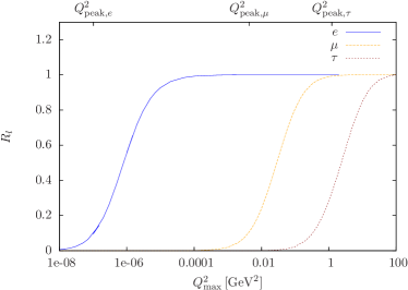
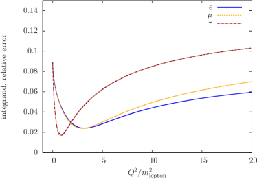
Figure 1: Upper plot: Comparison of the dependence on the upper integration bound in Eq. (5) of the four-flavour lepton anomalous magnetic moments. The blue curve represents the ratio defined in Eq. (10) for the electron, the orange one for the muon, and the dark red one for the tau. $Q^{2}_{{\rm peak},l}$ denotes the momentum value where the kernel function in Eq. (5) attains its maximum. Lower plot: Comparison of the dependence of the relative statistical uncertainties of the integrands in Eq. (5) on the squared momenta scaled by the lepton masses. The plots are based on data for the D30.48 ensemble featuring $a=0.061\,\mathrm{fm},\,m_{\mathrm{PS}}=318\,\mathrm{MeV}$, and $L=2.9\,\mathrm{fm}$.

This plot also implies that for the electron we have to rely mostly on the extrapolation of our vacuum polarisation data to the small momentum region. Although saturating well beyond momenta of $\mathcal{O}\left(1\,\mathrm{GeV}^{2}\right)$, also for the $\tau$, the renormalised vacuum polarisation function requires the subtraction of $\Pi(0)$, which is determined from the same extrapolation to the small momentum region.

Despite the different masses of the leptons, the lower plot of Fig. 1 shows that the relative statistical uncertainties are of the same orders of magnitude for all three leptons and display a universal dependence on $Q^{2}/m_{l}^{2}$.

3.1 Contribution from up and down quarks

The light quark contribution is depicted in Fig. 2. Here, we compare $a_{\rm e}^{ud}$ with the result at the physical value of the pion mass obtained with the standard definition Eq. (1) on one ensemble Abdel-Rehim:2013yaa ; Abdel-Rehim:2014nka with only one lattice spacing.

For the extrapolation in the upper plot of Fig. 2 we initially use $a_{\rm e}^{ud}$ from all our ensembles, i.e. all volumes, lattice spacings, and pion masses. As the figure shows, with the present accuracy of the data we do not resolve any statistically significant dependence of $a^{ud}_{e}$ on the lattice spacing or the lattice size. Using the modified definition (Eq. 5) with $H=m_{V}$ the ansatz

$$a_{\rm e}^{ud}\left(a,m_{\mathrm{PS}}^{2},L\right)=A+B\,m_{\mathrm{PS}}^{2}$$ (11)

is then already sufficient to describe our data. The result of this extrapolation is shown as the light grey band in Fig. 2. In principle, we are to add terms of higher order in $m_{\mathrm{PS}}^{2}$ for the extrapolation formula in Eq. (11),

$$a_{\rm e}^{ud}\left(a,m_{\mathrm{PS}}^{2},L\right)=A+B\,m_{\mathrm{PS}}^{2}+B_{2}\,m_{\mathrm{PS}}^{4}+\ldots$$ (12)

to account for any non-linear dependence on $m_{\mathrm{PS}}^{2}$. The dark grey band in the background in Fig. 2 shows the extrapolation with an additional term $B_{2}\,m_{\mathrm{PS}}^{4}$. The difference between this extrapolation and the previous one linear in the squared pion mass is insignificant. This insignificance of terms in $m_{\mathrm{PS}}^{2}$ beyond the linear one when using the improved definition in Eq. (5) turns out to be a universal property of $a_{\rm l}^{f}$ for all leptons and all flavour combinations $f=ud,udsc$ considered here and below. In addition, we check explicitly for lattice artefacts in the extrapolation by adding a term $C\,a^{2}$ to Eq. (11) with the result shown in the lower plot of Fig. 2.

We assume that lattice artefacts for the data at the physical point are negligible as well, which gives merit to the observed compatibility of the physical point result with the value determined by the linear extrapolation of the data described here.

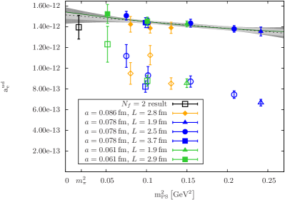
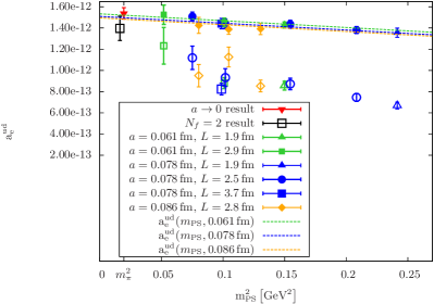
Figure 2: Upper plot: light-quark contribution to $a_{\rm e}^{\rm hvp}$ with filled symbols representing points obtained with Eq. (5), open symbols refer to those obtained with Eq. (1), i. e. $H=1$. In particular, the two-flavour result at the physical point has been computed with the standard definition. The light grey errorband belongs to the linear fit, whereas the dark grey errorband is attached to the quadratic fit. Lower plot: combined chiral and continuum extrapolation of the light-quark contribution to $a^{\mathrm{hlo}}_{\mathrm{e}}$ allowing for lattice artefacts.

3.2 Adding the strange and the charm quark contributions

When incorporating the heavy, second-generation flavours, which are described by the Osterwalder-Seiler action Osterwalder:1977pc ; Frezzotti:2004wz and whose masses have been tuned to their physical values as shown in Burger:2013jya , we take $\mathcal{O}(a^{2})$ lattice artefacts into account. The four-flavour result for $a_{\rm e}^{\rm hvp}$ at the physical point in the continuum limit is obtained from simultaneously extrapolating in the pion mass, $m_{\rm PS}$, and to zero lattice spacing $a$ using the ansatz

$$a_{\rm e}^{\rm hvp}\left(m_{\rm PS},a\right)=A+B\,m_{PS}^{2}+C\,a^{2}\,.$$ (13)

$A,B,C$ denote the free parameters of the fit. In the presence of the strange and charm contributions to $a_{\rm e}^{\rm hvp}$, the parameter $C$ will also contain terms $\sim m_{c,R}^{2},\,m_{s,R}^{2}$ from the renormalised charm and strange quark mass and also receives contributions from lattice artefacts possibly present in the light quark contribution to $a_{\rm e}^{\rm hvp}$. The reason for omitting a linear term in $a$ is that automatic $\mathcal{O}(a)$ improvement is retained for our definition of the hadronic vacuum polarisation function at maximal twist Burger:2014ada . As we have discussed in Burger:2013jya , systematic effects from varying the heavy valence and sea quark masses within the range given there have been found to be negligible. This is partly due to the contribution of strange and charm quark current correlators to vacuum polarisation being at least an order of magnitude smaller than those from the light quarks.

For $a_{\rm e}^{\rm hvp}$ the corresponding fit is shown in Fig. 3. Again we use data for $a_{\rm e}^{\rm hvp}$ for all lattice spacings, pion masses, and lattice volumes in this extrapolation. The ansatz in Eq. (13) is sufficient for a good description of all our data. This is shown by the three dashed lines, which evaluate the fit function for the individual lattice spacings. We have checked that amending the fit function by higher powers in $m_{\mathrm{PS}}^{2}$ does not lead to significantly different results for the extrapolated value. Comparing the results for different lattice volumes for lattice spacing $a=0.078\,\mathrm{fm}$ in Fig. 3 suggests the absence of observable finite volume effects. However, for the compilation of our complete error budget we investigate these effects in more detail below.

Our result with only statistical uncertainty is

$$a_{\rm e}^{\rm hvp}=1.78\,(06)\cdot 10^{-12}\;.$$ (14)

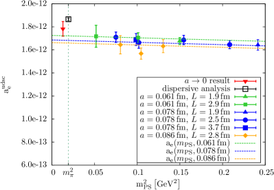
Figure 3: Chiral and continuum extrapolation of the $N_{f}=2+1+1$ contribution to $a_{\rm e}^{\rm hvp}$. The inverted red triangle shows the value extrapolated to the continuum and to the physical value of the pion mass. It has been displaced to the left to facilitate the comparison with the dispersive result in the black square Nomura:2012sb .

3.3 Systematic uncertainties

In this section, we give an account of systematic uncertainties of our result for $a_{\rm e}^{\rm hvp}$ given in Eq. (14). We have investigated finite size effects (FSE), the dependence of our chiral extrapolation on the incorporation of large pion masses, vector meson fit ranges, and the dependence of our results on different vacuum polarisation fit functions. Moreover, for one ensemble the light quark-disconnected contribution is quantified.

3.3.1 Finite size effects

As described in detail in Ref. Burger:2013jya , the $N_{f}=2+1+1$ ensembles analysed in this work feature $3.35<m_{\mathrm{PS}}~{}L<5.93$, where $L$ is the spatial extent of the lattice. Restricting our data to the condition $m_{\rm PS}L>3.8$ and $m_{\mathrm{PS}}L>4.5$, respectively, yields

$$a_{\rm e}^{\rm hvp}\left(m_{\mathrm{PS}}L>3.8\right) =1.77\,(07)\cdot 10^{-12}\;,$$ (15)

$$a_{\rm e}^{\rm hvp}\left(m_{\mathrm{PS}}L>4.5\right) =1.83\,(10)\cdot 10^{-12}\;,$$ (16)

after combined chiral and continuum extrapolation. This matches the result given in Eq. (14) and thus indicates that FSE are negligible in our computation. This finding is supported by comparing the results of two ensembles only differing in lattice size provided in Tab. 2. The numbers do not change when restricting the momenta of the larger ensemble to those of the smaller one. The FSE attributed to the lowest achievable momentum being $\frac{2\pi}{L}$ mixes with FSE entering the choice of different fit functions. We take a conservative approach and consider these effects separately.

Ensemble	$\left(\frac{L}{a}\right)^{3}\times\frac{T}{a}$	$a_{\mathrm{e,ud}}^{\mathrm{hvp}}$	$a_{\mathrm{e}}^{\mathrm{hvp}}$
B35.32	$32^{3}\times 64$	$1.44(05)\cdot 10^{-12}$	$1.66(05)\cdot 10^{-12}$
B35.48	$48^{3}\times 96$	$1.44(05)\cdot 10^{-12}$	$1.69(05)\cdot 10^{-12}$

Table 2: Comparison of light-quark contribution to $a_{\mathrm{e}}^{\rm hvp}$ and total $a_{\mathrm{e}}^{\mathrm{hvp}}$ from ensembles of different volumes.

3.3.2 Chiral extrapolation

We have checked the validity of the chiral extrapolation by restricting the data, comprising pion masses between $227\,{\rm MeV}$ and $491\,{\rm MeV}$, to the condition $m_{\rm PS}<400\,{\rm MeV}$. The value we obtain

$$a_{\rm e}^{\rm hvp}=1.78\,(07)\cdot 10^{-12}$$ (17)

only features a slightly larger uncertainty compared to the result in Eq. (14). Thus, we do not assign a systematic uncertainty to the usage of pion masses above $400\,{\rm MeV}$.

3.3.3 Vector meson fit ranges

Our standard computation involves the determination of the masses and decay constants of the vector meson ground states for the different flavours. Their values depend on the choice of fit ranges. We have analysed different fit ranges for the two-point functions of the light, strange, and charm vector currents and propagated the uncertainties to the values for $a_{\rm e}^{\rm hvp}$. This showed that excited state contaminations are significant only for $m_{V}$ and $f_{V}$ determined from the light vector current-current correlator. Variations of the standard fit ranges by $0.1\,{\rm fm}$ to the left, right and both simultaneously do not lead to any observable differences in $a_{\rm e}^{\rm hvp}$ for the $\overline{s}\gamma_{\mu}s$- and the $J/\psi$ correlator. Furthermore, the heavy flavour contributions are approximately one order of magnitude smaller than the light quark contribution such that their systematic uncertainties would not noticeably impact the overall uncertainty of $a_{\rm e}^{\rm hvp}$.

In the upper plot of Fig. 4, the dependence of the light quark contribution to the electron anomalous magnetic moment on the fitrange for the $\rho$-correlator is plotted. The lower limit $0.6\,\mathrm{fm}$ is a lower bound for the time region, where a single-state fit describes the 2-point correlation function. The upper end at $1.3\,\mathrm{fm}$ is less stringent, but the signal to noise ratio for the masses deteriorates quickly and the differences in a plot like Fig. 4 become insignificant.

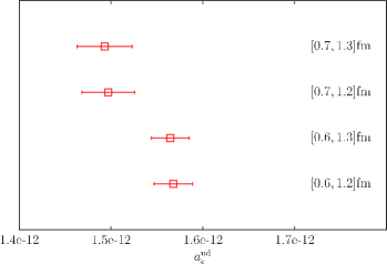
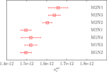
Figure 4: Dependence of $a_{\rm e}^{\rm ud}$ on the fitrange of the $\rho$-correlator (upper plot) and on values chosen for M, N in the vacuum polarisation fit function (lower plot). The standard $\rho$-correlator fit range is $[0.7\,{\rm fm},1.2\,{\rm fm}]$ and the standard fit function corresponds to M1N2.

Taking half the difference of the central values obtained for $[0.6\,{\rm fm},1.2\,{\rm fm}]$ and $[0.7\,{\rm fm},1.2\,{\rm fm}]$ gives a systematic uncertainty of

$$\Delta_{V}=0.035\cdot 10^{-12}\;.$$ (18)

3.3.4 Number of terms in MN fit function

The number of terms in the fit function Eq. (7) is given by M and N. M1N2 is our standard choice. Repeating the whole analysis with different numbers of terms for the light quark contribution leads to the results shown in the lower plot of Fig. 4. We observe that the chirally and continuum extrapolated results of fit functions involving one and two poles are not compatible and thus we assign a systematic error by taking half the difference of the central values of the result of the M2N3 and the M1N2 fit. This leads to a systematic uncertainty of

$$\Delta_{MN}^{\rm ud}=0.071\cdot 10^{-12}\;.$$ (19)

This results in the dominant systematic uncertainty of the determination of $a_{\rm e}^{\rm hvp}$. For the strange quark the systematic uncertainty from different values of M and N is

$$\Delta_{MN}^{\rm s}=0.007\cdot 10^{-12}\;$$ (20)

which we add to the light quark one. The differences of results from different fit functions for the charm quark contribution have turned out to be negligible such that the total systematic error originating from employing various numbers of terms in the fit function amounts to

$$\Delta_{MN}=0.078\cdot 10^{-12}\;.$$ (21)

3.3.5 Disconnected contributions

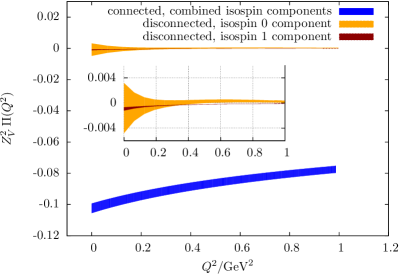
Figure 5: Comparison of the light quark contributions to the unsubtracted hadronic vacuum polarisation function from quark-connected and disconnected diagrams of the local current correlator. $Z_{V}$ has been obtained from the ratio of the connected part of the conserved and local current-current correlators. The values have been computed with the analytical continuation method described in Feng:2013xsa without correcting for finite-size effects.

Leaving out the quark-disconnected contributions is a systematic uncertainty we cannot completely quantify, yet. We have started investigating their magnitude on the B55.32 ensemble mentioned already before. Using the local vector current we have detected a signal for the light quark part of the vacuum polarisation function when using 24 stochastic volume sources on 1548 configurations and 48 stochastic volume sources on 4996 configurations. Employing the one-end trick Boucaud:2008xu , the isovector part

$$\Pi^{3}_{\mu\nu}(x,y)=\langle J_{\mu}^{3}(x)J_{\nu}^{3}(y)\rangle$$ (22)

with $J_{\mu}^{3}=\frac{1}{2}\overline{\chi}\gamma_{\mu}\tau^{3}\chi$ is significantly different from zero. However, this is a pure lattice artefact and will not contribute in the continuum limit. On the other hand, the more interesting isoscalar part

$$\Pi^{0}_{\mu\nu}(x,y)=\frac{1}{9}\langle J_{\mu}^{0}(x)J_{\nu}^{0}(y)\rangle$$ (23)

with $J_{\mu}^{0}=\frac{1}{2}\overline{\chi}\gamma_{\mu}\mathds{1}\chi$ is compatible with zero. The connected and disconnected pieces of the polarisation function for the light flavours are depicted in Fig. 5.

A comparison of the values of $a_{l,\rm ud}^{\rm hvp}$ for all three leptons on the B55.32 ensemble with and without incorporating the disconnected contributions is presented in Tab. 3. Here, we have combined the connected pieces obtained from the point-split current correlator with the isoscalar part of the disconnected contributions obtained from the local current correlator using the renormalisation constant $Z_{V}$ determined from the ratio of the connected pieces of the conserved and the local vector current two-point functions. Therefore and because we only have results for one ensemble, the numbers below can only give hints on the influence of the disconnected pieces. We observe the tendency that for all three leptons $a_{l,\rm ud}^{\rm hvp}$ decreases when incorporating the disconnected contributions as has been predicted in DellaMorte:2010aq . However, this is statistically not significant. Furthermore, we find that the magnitude of the disconnected contributions is comparable to our current uncertainty. Hence, it will be mandatory to compute them when aiming at more precise results. For the muon the value shifts by $\approx 3\%$, which is also not statistically significant at this stage, but is in accordance with the upper bound of $4-5\%$ given in Francis:2014hoa as well as more recent high-statistics evaluations in Toth:2015lat ; Blum:2015you .

	without disc	with disc
$a_{\mathrm{e,ud}}^{\mathrm{hvp}}$	$1.44(04)\cdot 10^{-12}$	$1.39(07)\cdot 10^{-12}$
$a_{\mathrm{\mu,ud}}^{\mathrm{hvp}}$	$5.42(14)\cdot 10^{-8}$	$5.26(25)\cdot 10^{-8}$
$a_{\mathrm{\tau,ud}}^{\mathrm{hvp}}$	$1.27(03)\cdot 10^{-6}$	$1.24(04)\cdot 10^{-6}$

Table 3: Comparison of light-quark contributions to $a_{l}^{\rm hvp}$ with and without disconnected pieces in the low-momentum region for the B55.32 ensemble. For all contributions the redefinition Eq. (5) and our standard analysis have been used.

The disconnected heavy flavour contributions need to be considered as well. We plan to check their size in future calculations. The pure charm quark contributions have been computed in perturbation theory and shown to be suppressed by a factor $\left(\frac{q^{2}}{4~{}m_{c}^{2}}\right)^{4}$ Groote:2001py , where $q^{2}$ is the relevant energy scale of the problem.

3.4 Comparison with the phenomenological value

Adding the quantified systematic uncertainties in quadrature we obtain as final result

$$a_{\rm e}^{\rm hvp}=1.782\,(64)(86)\cdot 10^{-12}\;.$$ (24)

This can directly be compared with the phenomenological determination of Nomura:2012sb

$$a_{\rm e}^{\rm hvp}=1.866\,(10)\,(05)\cdot 10^{-12}\;.$$ (25)

They are fully compatible with each other although our lattice result still is afflicted with larger errors.

4 The $\tau$-lepton $(g-2)$

The large mass of the tau lepton, $m_{\tau}\approx 1.8\,{\rm GeV}$, implies a peak of the weight function in the expression for the LO hadronic contribution to its magnetic moment in Eq. (1) at $Q_{\rm peak}^{2}=0.745\,{\rm GeV}^{2}$. This is very different from the peak position of the electron weight function. Hence, the saturation of $a_{\rm\tau}^{\rm hvp}$ requires data from a different part of the subtracted vacuum polarisation function, in particular, also the high-momentum piece of our fit function Eq. (8) is important here.

4.1 Contribution from up an down quarks

As for the electron, we start off by showing the contribution of the first-generation flavours to $a_{\rm\tau}^{\rm hvp}$ in the upper plot of Fig. 6. The data show a qualitatively similar behaviour to those of the electron in Fig. 2. Their values differ, however, by six orders of magnitude. In particular, by comparing the upper and lower plot of Fig. 6 we find that no significant lattice artefacts are present and that the data at unphysical pion masses obtained with Eq. (5), can be linearly extrapolated to the physical point. This demonstrates again that the method of including $\frac{H}{H_{\rm phys}}$ in the weight function is advantageous for the chiral extrapolation. The value extrapolated in this way and using all available lattice ensembles agrees with our calculation directly at the physical pion mass shown as the open square in Fig. 6.

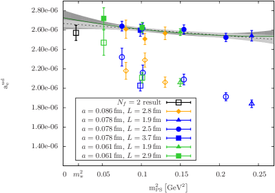
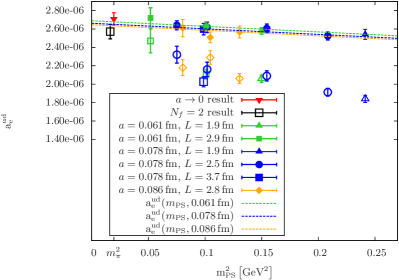
Figure 6: Upper plot: light-quark contribution to $a_{\rm\tau}^{\rm hvp}$ with filled symbols representing points obtained with Eq. (5), open symbols refer to those obtained with Eq. (1), i. e. $H=1$. We note that the two-flavour result at the physical point has been computed with the standard definition. The light grey errorband belongs to the linear fit (dotted black line), whereas the dark grey errorband is attached to the quadratic fit (solid green line). Lower plot: combined chiral and continuum extrapolation taking into account leading order lattice artefacts.

4.2 Adding the strange and the charm quark contributions

As for the electron, we perform the chiral and continuum extrapolation of the complete four-flavour result using a fit of the form given in Eq. (13) and data for all lattice spacings, pion masses, and lattice volumes simultaneously. It is shown in Fig. 7. Comparing this with Fig. 3, we see that the lattice artefacts are much smaller than for the electron such that we would have obtained a compatible result when omitting the $a^{2}$ term in Eq. (13). As can be seen in Figs. 9 and 9, for the tau lepton both, the strange and the charm contribution do not show significant cut-off effects and hence, also for the total contribution $a^{2}$ effects are small. We nevertheless perform the continuum extrapolation in order to use exactly the same analysis strategy as for the other leptons.

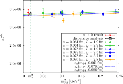
Figure 7: Chiral and continuum extrapolation of the $N_{f}=2+1+1$ contribution to $a_{\rm\tau}^{\rm hvp}$. The inverted red triangle shows the value in the continuum limit at the physical value of the pion mass. It has been displaced to the left to facilitate the comparison with the dispersive result depicted as black square Eidelman:2007sb .

Figure 8: Continuum limit of strange quark contribution to $a_{\rm\tau}^{\rm hvp}$ at approximately fixed pion mass.

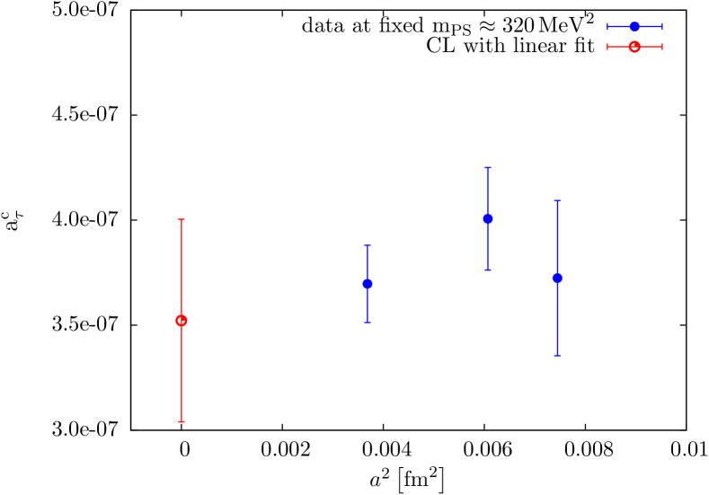
Figure 9: Continuum limit of charm quark contribution to $a_{\rm\tau}^{\rm hvp}$ at approximately fixed pion mass.

Our four-flavour result with only statistical uncertainty reads

$$a_{\rm\tau}^{\rm hvp}=3.41\,(8)\cdot 10^{-6}\,.$$ (26)

4.3 Systematic uncertainties

We have investigated the same systematic uncertainties for our determination of $a_{\tau}^{\rm hvp}$ as for the case of the electron. The influence of the disconnected contributions has already been discussed in the section of $a_{\rm e}^{\rm hvp}$.

4.3.1 Finite size effects

Restricting our data to the conditions $m_{\rm PS}L>3.8$ and $m_{\mathrm{PS}}L>4.5$ yields

$$a_{\rm\tau}^{\rm hvp}\left(m_{\mathrm{PS}}L>3.8\right) =3.40\,(09)\cdot 10^{-6}\;,$$ (27)

$$a_{\rm\tau}^{\rm hvp}\left(m_{\mathrm{PS}}L>4.5\right) =3.54\,(13)\cdot 10^{-6}\;.$$ (28)

This is compatible with the result in Eq. (26). Comparing again the two ensembles at $m_{\rm PS}\approx 315\,{\rm MeV}$ which only differ in the extent of the lattices also indicates negligible finite size effects as shown in Tab. 4. Hence, we do not assign a FSE related systematic uncertainty.

Ensemble	$\left(\frac{L}{a}\right)^{3}\times\frac{T}{a}$	$a_{\mathrm{\tau,ud}}^{\mathrm{hvp}}$	$a_{\mathrm{\tau}}^{\mathrm{hvp}}$
B35.32	$32^{3}\times 64$	$2.62\,(06)\cdot 10^{-6}$	$3.40\,(07)\cdot 10^{-6}$
B35.48	$48^{3}\times 96$	$2.60\,(06)\cdot 10^{-6}$	$3.41\,(07)\cdot 10^{-6}$

Table 4: Comparison of light-quark contribution to $a_{\mathrm{\tau}}^{\rm hvp}$ and total $a_{\mathrm{\tau}}^{\mathrm{hvp}}$ from ensembles of different volumes.

4.3.2 Chiral extrapolation

Restricting the analysed ensembles to those featuring pion masses $m_{\rm PS}<400\,{\rm MeV}$, we get

$$a_{\rm\tau}^{\rm hvp}=3.45\,(09)\cdot 10^{-6}\;.$$ (29)

This is again compatible with the value given in Eq. (26). Hence, we do not assign a systematic uncertainty to the fact that ensembles with pion masses above $400\;{\rm MeV}$ have been employed when extrapolating to the physical value of the pion mass.

4.3.3 Vector meson fit ranges

The situation is similar to the case of the electron reported above. Only the excited state contamination in the $\rho$-correlator has to be taken into account as systematic uncertainty. In the upper plot of Fig. 10 the dependence of the light quark contribution, $a_{\rm\tau}^{\rm ud}$, on the fit range chosen to extract the spectral information from the $\rho$-correlator is depicted.

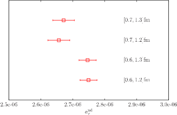
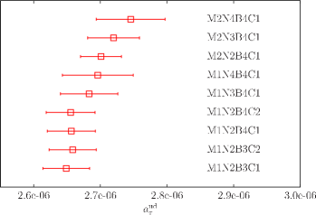
Figure 10: Dependence of $a_{\rm\tau}^{\rm ud}$ on the fit range of the $\rho$-correlator (upper plot) and on the values chosen for M, N, B, and C in the vacuum polarisation fit function (lower plot). The standard $\rho$-correlator fit range is $[0.7\,{\rm fm},1.2\,{\rm fm}]$ and the standard fit function corresponds to M1N2B4C1.

Taking half the difference of the central values obtained for $[0.6\,{\rm fm},1.2\,{\rm fm}]$ and our standard fit range $[0.7\,{\rm fm},1.2\,{\rm fm}]$ results in an estimated systematic uncertainty of

$$\Delta_{V}=0.046\cdot 10^{-6}\;.$$ (30)

4.3.4 Number of terms in MNBC fit function

Due to the large $Q^{2}_{\rm peak}$ we have to take the whole vacuum polarisation function Eq. (9) into account, including in particular the high-momentum piece in Eq. (8). Thus, we have four different types of terms in the fit function that can have different numbers of summands. We only find observable differences in the light quark sector. But also here the results from different fits are all compatible as shown in the lower plot of Fig. 10. Conservatively, we take half the difference between the M2N3B4C1 and M1N2B4C1 fit and assign a systematic uncertainty of

$$\Delta_{MNBC}=0.032\cdot 10^{-6}$$ (31)

to our choice of the fit function.

4.4 Comparison with the phenomenological value

Including the identified systematic uncertainties added in quadrature, our final four-flavour result reads

$$a_{\rm\tau}^{\rm hvp}=3.41\,(8)(6)\cdot 10^{-6}\,.$$ (32)

This agrees with the one obtained by a dispersive analysis Eidelman:2007sb

$$a_{\rm\tau}^{\rm hvp}=3.38\,(4)\cdot 10^{-6}\;.$$ (33)

Compared to the electron, even better agreement between the lattice and the phenomenological result is observed for the $\tau$-lepton. In this case, the uncertainty of our twisted mass LQCD calculation is only about twice the phenomenological one.

5 Summary and Conclusions

In this article we have presented the first four-flavour LQCD computation of the LO hadronic vacuum polarisation contributions to the anomalous magnetic moments of the electron and the $\tau$-lepton. Our results have been obtained with $N_{f}=2+1+1$ twisted mass fermions mostly at unphysically large pion masses but, at least for the light quark contribution, also directly at the physical point. We find that for both, the electron and the tau lepton, the chirally extrapolated values for the light quark contributions agree with the one at the physical point.

For our data at unphysically large values of the pion mass we have investigated the systematic uncertainties of the method used to obtain our final results. In particular, we have addressed the effects of non-zero lattice spacings, the finite volumes, the fit range for extracting the vector meson mass, and using different fit functions for the vacuum polarisation function. As an additional uncertainty we have investigated the disconnected contributions on one of our 4-flavor ensembles (B55.32) by using the local vector current. This led to the first observation of a signal for the disconnected diagrams during our calculations, which, however, is compatible with zero within our current errors and which we therefore have neglected. This will no longer be justified once the uncertainties of the connected pieces are reduced and a full quantification of the quark-disconnected contribution will become significant.

Our final results are summarised in Tab. 5 below and agree with the phenomenological determinations of the electron and tau lepton magnetic moments which are also shown there. This universal agreement across all three leptons and thus distinct weightings of the subtracted polarisation functions is elucidated by our findings in Ref. Burger:2015lqa . There it was shown, that the subtracted vacuum polarisation function itself calculated with the methods used in this work and described in more detail in Ref. Burger:2013jya , is compatible with the phenomenological result for $\Pi_{R}(Q^{2})$ in the range $0\leq Q^{2}\leq\mathcal{O}\left(10\,\mathrm{GeV}^{2}\right)$.

	this work	dispersive analyses
$a_{\mathrm{e}}^{\rm hvp}$	$1.782\,(64)(86)\cdot 10^{-12}$	$1.866\,(10)\,(05)\cdot 10^{-12}$	Nomura:2012sb
$a_{\mathrm{\mu}}^{\mathrm{hvp}}$	$6.78\,(24)(16)\cdot 10^{-8}$	$6.91\,(01)\,(05)\cdot 10^{-8}$	Jegerlehner:2011ti
$a_{\mathrm{\tau}}^{\mathrm{hvp}}$	$3.41\,(8)(6)\cdot 10^{-6}$	$3.38\,(4)\cdot 10^{-6}$	Eidelman:2007sb

Table 5: Comparison of our first-principle values for $a_{\mathrm{e}}^{\rm hvp}$, $a_{\mathrm{\mu}}^{\mathrm{hvp}}$, and $a_{\mathrm{\tau}}^{\mathrm{hvp}}$ with phenomenological results.

As expected from the graph in the lower plot of Fig. 1 the relative statistical uncertainties in all three cases are similar. For the electron the systematic uncertainty already exceeds the statistical one.

As in the case of the muon, also for the electron and tau lepton anomalous magnetic moments the errors of our calculations are still larger than those from the dispersive analyses quoted above. However, it can be expected that with future lattice QCD calculations at the physical value of the pion mass, increased statistics and an even better control over systematic uncertainties the phenomenological error can be matched, if not even beaten, especially for the $\tau$-lepton.

- (1) K. Olive, et al., Chin.Phys. C38, 090001 (2014). DOI 10.1088/1674-1137/38/9/090001
- (2) D. Hanneke, S. Fogwell, G. Gabrielse, Phys.Rev.Lett. 100, 120801 (2008). DOI 10.1103/PhysRevLett.100.120801
- (3) T. Aoyama, M. Hayakawa, T. Kinoshita, M. Nio, Phys.Rev.Lett. 109, 111808 (2012). DOI 10.1103/PhysRevLett.109.111808
- (4) T. Aoyama, M. Hayakawa, T. Kinoshita, M. Nio, Phys.Rev. D91(3), 033006 (2015). DOI 10.1103/PhysRevD.91.033006
- (5) G. Giudice, P. Paradisi, M. Passera, JHEP 1211, 113 (2012). DOI 10.1007/JHEP11(2012)113
- (6) N. Brambilla, S. Eidelman, P. Foka, S. Gardner, A. Kronfeld, et al., Eur.Phys.J. C74(10), 2981 (2014). DOI 10.1140/epjc/s10052-014-2981-5
- (7) J. Abdallah, et al., Eur.Phys.J. C35, 159 (2004). DOI 10.1140/epjc/s2004-01852-y
- (8) T. Aoyama, M. Hayakawa, T. Kinoshita, M. Nio, Phys.Rev.Lett. 109, 111807 (2012). DOI 10.1103/PhysRevLett.109.111807
- (9) A. Czarnecki, B. Krause, W.J. Marciano, Phys.Rev. D52, 2619 (1995). DOI 10.1103/PhysRevD.52.R2619
- (10) A. Czarnecki, B. Krause, W.J. Marciano, Phys.Rev.Lett. 76, 3267 (1996). DOI 10.1103/PhysRevLett.76.3267
- (11) S.F. Hoogerheide, J. Dorr, E. Novitski, G. Gabrielse, (2014)
- (12) A. Pich, Prog.Part.Nucl.Phys. 75, 41 (2014). DOI 10.1016/j.ppnp.2013.11.002
- (13) M. Fael, L. Mercolli, M. Passera, Nucl.Phys.Proc.Suppl. 253-255, 103 (2014). DOI 10.1016/j.nuclphysbps.2014.09.025
- (14) B. Oberhof, Nucl.Part.Phys.Proc. 260, 12 (2015). DOI 10.1016/j.nuclphysbps.2015.02.003
- (15) F. Burger, X. Feng, G. Hotzel, K. Jansen, M. Petschlies, et al., JHEP 1402, 099 (2014). DOI 10.1007/JHEP02(2014)099
- (16) M. Benayoun, P. David, L. DelBuono, F. Jegerlehner, Eur.Phys.J. C73, 2453 (2013). DOI 10.1140/epjc/s10052-013-2453-3
- (17) B. Colquhoun, R. Dowdall, C. Davies, K. Hornbostel, G. Lepage, (2014)
- (18) R. Baron, P. Boucaud, J. Carbonell, A. Deuzeman, V. Drach, et al., JHEP 1006, 111 (2010). DOI 10.1007/JHEP06(2010)111
- (19) R. Baron, et al., Comput.Phys.Commun. 182, 299 (2011). DOI 10.1016/j.cpc.2010.10.004
- (20) A. Abdel-Rehim, P. Boucaud, N. Carrasco, A. Deuzeman, P. Dimopoulos, et al., PoS LATTICE2013, 264 (2013)
- (21) A. Abdel-Rehim, C. Alexandrou, P. Dimopoulos, R. Frezzotti, K. Jansen, et al., PoS LATTICE2014, 119 (2014)
- (22) X. Feng, K. Jansen, M. Petschlies, D.B. Renner, Phys.Rev.Lett. 107, 081802 (2011). DOI 10.1103/PhysRevLett.107.081802
- (23) D.B. Renner, X. Feng, K. Jansen, M. Petschlies, (2012)
- (24) B. Lautrup, A. Peterman, E. de Rafael, Phys.Rept. 3, 193 (1972). DOI 10.1016/0370-1573(72)90011-7
- (25) T. Blum, Phys.Rev.Lett. 91, 052001 (2003). DOI 10.1103/PhysRevLett.91.052001
- (26) F. Burger, G. Hotzel, K. Jansen, M. Petschlies, JHEP 1503, 073 (2015). DOI 10.1007/JHEP03(2015)073
- (27) C. Aubin, T. Blum, M. Golterman, S. Peris, Phys.Rev. D86, 054509 (2012). DOI 10.1103/PhysRevD.86.054509
- (28) M. Golterman, K. Maltman, S. Peris, Phys.Rev. D88(11), 114508 (2013). DOI 10.1103/PhysRevD.88.114508
- (29) F. Burger, G. Hotzel, K. Jansen, M. Petschlies, PoS LATTICE2014, 145 (2014)
- (30) M. Marinkovic, P. Boyle, L. Del Debbio, A. Juettner, K. Maltman, et al., (2015)
- (31) R. Baron, et al., PoS LATTICE2010, 123 (2010)
- (32) A. Abdel-Rehim, et al., (2015)
- (33) K. Osterwalder, E. Seiler, Annals Phys. 110, 440 (1978). DOI 10.1016/0003-4916(78)90039-8
- (34) R. Frezzotti, G.C. Rossi, JHEP 10, 070 (2004)
- (35) D. Nomura, T. Teubner, Nucl.Phys. B867, 236 (2013). DOI 10.1016/j.nuclphysb.2012.10.001
- (36) X. Feng, S. Hashimoto, G. Hotzel, K. Jansen, M. Petschlies, et al., Phys.Rev. D88, 034505 (2013). DOI 10.1103/PhysRevD.88.034505
- (37) P. Boucaud, et al., Comput. Phys. Commun. 179, 695 (2008). DOI 10.1016/j.cpc.2008.06.013
- (38) M. Della Morte, A. Juttner, JHEP 1011, 154 (2010). DOI 10.1007/JHEP11(2010)154
- (39) A. Francis, V. Gülpers, B. Jäger, H. Meyer, G. von Hippel, et al., PoS LATTICE2014, 128 (2014)
- (40) B. Toth, (2015)
- (41) T. Blum, P.A. Boyle, T. Izubuchi, L. Jin, A. Juettner, C. Lehner, K. Maltman, M. Marinkovic, A. Portelli, M. Spraggs, (2015)
- (42) S. Groote, A. Pivovarov, JETP Lett. 75, 221 (2002). DOI 10.1134/1.1478517
- (43) S. Eidelman, M. Passera, Mod.Phys.Lett. A22, 159 (2007). DOI 10.1142/S0217732307022694
- (44) F. Burger, K. Jansen, M. Petschlies, G. Pientka, JHEP 11, 215 (2015). DOI 10.1007/JHEP11(2015)215
- (45) F. Jegerlehner, R. Szafron, Eur.Phys.J. C71, 1632 (2011). DOI 10.1140/epjc/s10052-011-1632-3
- (46) C. Michael, K. Ottnad, C. Urbach, Phys.Rev.Lett. 111(18), 181602 (2013). DOI 10.1103/PhysRevLett.111.181602