Radio-X-ray synergy to discover and study jetted tidal disruption events

Abstract

Observational consequences of tidal disruption of stars (TDEs) by supermassive black holes (SMBHs) can enable us to discover quiescent SMBHs, constrain their mass function, study formation and evolution of transient accretion disks and jet formation. A couple of jetted TDEs have been recently claimed in hard X-rays, challenging jet models, previously applied to $\gamma$-ray bursts and active galactic nuclei. It is therefore of paramount importance to increase the current sample. In this paper, we find that the best strategy is not to use up-coming X-ray instruments alone, which will yield between several (e-Rosita) and a couple of hundreds (Einstein Probe) events per year below redshift one. We rather claim that a more efficient TDE hunter will be the Square Kilometer Array (SKA) operating in survey mode at 1.4 GHz. It may detect up to several hundreds of events per year below $z\sim 2.5$ with a peak rate of a few tens per year at $z\approx 0.5$. Therefore, even if the jet production efficiency is not $100\%$ as assumed here, the predicted rates should be large enough to allow for statistical studies. The characteristic TDE decay of $t^{-5/3}$, however, is not seen in radio, whose flux is quite featureless. Identification therefore requires localization and prompt repointing by higher energy instruments. If radio candidates would be repointed within a day by future X-ray observatories (e.g. Athena and LOFT-like missions), it will be possible to detect up to $\approx 400$ X-ray counterparts, almost up to redshift $2$. The shortcome is that only for redshift below $\approx 0.4$ the trigger times will be less than 10 days from the explosion. In this regard the X-ray surveys are better suited to probe the beginning of the flare, and are therefore complementary to SKA.

1 Introduction

Since the late 70s it has been suggested that stars torn apart by the gravitational field of a supermassive black hole (SMBH) may be observed as flares from Earth (Hills, 1975; Frank & Rees, 1976; Rees, 1988; Phinney, 1989). These are called tidal disruption events (TDEs). These flares would be caused by sudden accretion of the star debris, which would feed the SMBH at an ever decreasing rate, $\dot{M}\propto t^{-5/3}$. This theoretical expectation is for a complete disruption of a star in parabolic orbit, after at least several days from the peak (e.g. Lodato et al., 2009; Hayasaki et al., 2013; Guillochon & Ramirez-Ruiz, 2013), and it is expected to be independent on the ratio of pericenter to tidal radius (Sari et al., 2010; Stone et al., 2013).

The detection and study of these flares can deliver important astrophysical information. On the one hand, they allow us to detect otherwise quiescent SMBHs and estimate their masses. This would inform theory of galaxy-SMBH cosmological co-evolution. On the other, they constitute a unique opportunity to study the – highly theoretically uncertain – formation of an accretion disc and its continuous transition through different accretion states. As the accretion rate decreases, we can in principle observe a disc which transits from an initial super-Eddington phase, lasting several months, passing through a slim and later a thin disc regime, and ending its life, years later, in a radiative inefficient state. The super-Eddington phase –which occurs only for SMBH masses $\lower 2.15277pt\hbox{$\;\buildrel<\over{\sim}\;$}10^{7}$ M_⊙ — is highly uncertain, but it may be associated with a copious radiative driven wind (Rossi & Begelman, 2009), which thermally emits $\sim 10^{41}-10^{43}$ erg s^-1, mainly at optical frequencies (Strubbe & Quataert, 2009; Lodato & Rossi, 2011). The disc luminosity ($\sim 10^{45}-10^{46}$ erg s^-1), instead, peaks in far-UV/soft X-rays (Lodato & Rossi, 2011). Of paramount theoretical importance would also be the possibility to investigate the formation and evolution of an associated jet, powered by this sudden accretion. There is no specific theory for the jet emission from TDEs. Astronomers mainly assume a phenomenological description (e.g. Van Velzen et al., 2011; Canizzo et al., 2011) or borrow theory developed for blazars and/or $\gamma$-ray bursts (e.g. Metzger et al., 2012; Tchekhovskoy et al., 2013). In general, non-thermal emission in X-rays and radio is the jet signature.

Handful of candidate TDEs ($\sim 10$) have been detected so far, particularly in ROSAT all sky survey (Komossa, 2002; Donley et  al., 2002), in GALEX Deep Imaging Survey (Gezari  et  al., 2009; Gezari et al., 2012; Campana et al., 2011) and in SDSS (Van Velzen et  al., 2011a). These “soft” events are believed to be associated with the disc and wind thermal emission. The presence of a bright optical flare in the initial super-Eddington months makes optical surveys a useful tool for discovery. Significant advances in optical transient surveys are expected to be achieved by the Panoramic Survey Telescope and Response System (Pan-STARRS) and the Large Synoptic Survey Telescope (LSST). Two candidates have been claimed in Pan-STARRS data (Gezari et al., 2012; Chornock et al., 2014), three in PTF data (Arcavi et al., 2014) and one in ASAS-SN (Holoien et al., 2014), but the total number expected seems to be much higher. For example in the $3\pi$ Survey, claims in literature range from 200 to $\sim 1557$, while in the medium deep survey there is more consensus that $\sim 15-20$ should be found (Strubbe & Quataert, 2009; Van Velzen et  al., 2011a). Thousands of candidates could be, instead, detected by LSST, with its 6-band ($0.3-1.1$ micron) wide-field deep astronomical survey of over 20000 square degrees of the southern sky, using an $8.4$-meter ground-based telescope (Strubbe & Quataert, 2009; Van Velzen et  al., 2011a). However, these estimates are probably upper limits, because galactic nuclei can heavily absorb optical light.

More recently, two candidates TDEs were triggered in the hard X-ray band by the BAT instrument on board of Swift (Bloom et al., 2011; Burrows et al., 2011; Cenko et al., 2012). A multi-frequency follow-up from radio to $\gamma$-rays revealed a new class of TDEs, where we are likely observing the non-thermal emission from a relativistic jet. The jet emission is responsible for the hard X-ray spectrum (with power-law slope $\beta\sim 1.7$) and the increasing radio activity (Levan et al., 2011), detected a few days after the trigger.

Given the lack of statistics and of a solid theoretical framework for the non-thermal emission, we will take the best studied of these two events, Swift J1644+57 (Sw J1644 in short), as a prototype for the study presented in this paper, where we investigate the detection capability of both SKA and future X-ray observatories.

Sw J1644 was hosted by a star forming galaxy at $z=0.354$ and in positional coincidence with its center (Zauderer et al., 2011). Its X-ray peak luminosity $\sim 3\times 10^{48}$ erg s^-1 was reached after a couple of days from the trigger, and it persisted at the level of $>10^{45}$ erg s^-1 for about 1 year. During its decay, the X-ray emission was approximately described by a $t^{-5/3}$ temporal law, the same as that expected for the fallback of stellar debris (see Figure 1). After $\sim 500$ day from the trigger, the X-ray flux declined by two orders of magnitude and it has been associated with a shut off of the relativistic jet (Zauderer et al., 2013). The modelling of the X-ray luminosity suggests that Sw J1644 is associated with a light supermassive black hole $\lower 2.15277pt\hbox{$\;\buildrel<\over{\sim}\;$}10^{7}M_{\sun}$ (e.g. Burrows et al., 2011; Canizzo et al., 2011).

Variability at optical wavelengths within the host was not detected, while transient emission was seen in infrared, becoming stronger at longer wavelengths, especially at millimeter and radio wavelengths. Radio (1.4. and 4.8 GHz) observations from Westerbork Synthesis Radio Telescope (WSRT) showed a bright source. EVLA observations of the radio transient coincident with the host galaxy were reported, providing an estimate of the bulk Lorentz factor $\Gamma\sim 2$ of the outflow (Zauderer et al., 2011). The radio lightcurve displays a rebrightening starting one month after the trigger (Berger et al., 2012; Zauderer et al., 2013). The emission peaks around several months, followed by a decline. Radio observations stop at 600 days after the trigger (Zauderer et al., 2013). The radio behavior is not compatible with the blast wave model borrowed from $\gamma$-ray bursts by Metzger et al. (2012), and indicate a more complicated jet structure, like perhaps in the magnetically arrested model proposed by Tchekhovskoy et al. (2013). Snapshot rates of jetted TDEs in radio band have been computed for the first time by Van Velzen et al. (2011). Differently from their work, we adopt here a different modelling for the radio lightcurve and a more detailed one for the black hole mass function, which includes the redshift dependence. We also account for a stellar mass function. We broaden up our investigation to include X-ray detection and follow-ups.

Finally, a 200-s quasi-periodic oscillation (QPO) was detected by both Suzaku and XMM, $\sim 10$ and 19 days after the Swift/BAT trigger, respectively (Reis et al., 2012). QPOs are regularly detected in stellar mass BHs, but there is no firm physical interpretation of these phenomena. However, most models strongly link the origin of high-frequency QPOs with orbits or resonances in the inner accretion disk close to the BH. This may cause variable energy injection into the jet, which consequently results in variability in the X-ray emission. This interpretation led to estimate a BH mass between $5\times 10^{5}M_{\odot}$ and $5\times 10^{6}M_{\odot}$ (Reis et al., 2012).

In this paper, we predict the detection rate of jetted TDEs considering current and future radio surveys (NVSS + FIRST, VLT Stripe 82, ASKAP, VLASS and SKA) and X-ray instruments (Swift, eRosita, Einstein Probe, Athena, LOFT). In addition, we discuss the ability of these instruments to constrain important physical parameters.

The paper is organized as follows. In §2, we take Swift J1644 as a prototype and we describe our phenomenological model for X-ray and Radio emissions. In §3, we discuss the black hole distribution functions used in this paper. In §4, we present our Monte Carlo calculations. Our rates for current and future surveys are presented in §5. A summary and implications of our results can be found in §6. Finally, we draw our conclusions in §7.

Throughout this paper we use the following cosmological parameters: $\Omega_{\rm M}=0.25$, $\Omega_{\rm\lambda}=0.75$ and $H_{\rm 0}=70~{}{\rm km/s/Mpc}$.

2 Modelling the Lightcurve

A tidal disruption event of a star by a SMBH causes a transient accretion disc to form, whose accretion rate is set by the rate at which the stellar debris falls back to the black hole under its gravitational pull. How matter circularizes to form a disc and whether this process is accompanied by outflows and their characteristics are subject to intense investigations, as mentioned above. From phenomenology and theory, we know that in the presence of an accretion disc and some ordered magnetic field, matter and energy outflows in form of (relativistic) jets are produced. In the absence of fully consistent simulations of jet production by a tidal disruption event, we use below a simplified description for the jet energy content as a function of time. This is partially supported by analytical and numerical calculations (see references above) and partly by the observed features of the X-ray emission of Sw J1644. In particular, its temporal decay ($\sim t^{-5/3}$) suggests that at least in this optically thin regime, the X-ray luminosity scales as the accretion rate. As a consequence, it supports a scenario in which the star was completely tidally disrupted, since partial disruption would lead to a shallower decay of the fallback rate (Guillochon & Ramirez-Ruiz, 2013). Moreover, a partial disruption is difficult to reconcile with a long lasting super Eddington accretion phase, which may be needed to power the jet for its total duration of $\sim 500$ days. Finally, the modelling of the X-ray luminosity suggests that Sw J1644 is the consequence of a disruption of a roughly one solar mass star by a light supermassive black hole $\lower 2.15277pt\hbox{$\;\buildrel<\over{\sim}\;$}10^{7}M_{\sun}$ (e.g. Burrows et al., 2011; Canizzo et al., 2011).

2.1 Jet kinetic power

We work in the framework of two identical jets, with $\theta_{\rm j}<1/\Gamma$. The total energy injected in the two jets is $L_{\rm j}=\epsilon_{\rm j}\dot{M}_{\rm fb}c^{2}$, where $\epsilon_{\rm j}$ is the jet production efficiency, which we assume constant in time, and the gas fall back to form a disc occurs at a rate $\dot{M}_{\rm fb}$. For a complete disruption of a star in parabolic orbit the fallback rate can be approximated by

$$\dot{M}_{\rm fb}(\bar{\tau})=\dot{M}_{\rm p}\left(\frac{t_{\rm min}+\bar{\tau}}{t_{\rm min}}\right)^{-5/3},$$ (1)

(Rees, 1988; Phinney, 1989). The lag time “$\bar{\tau}$” is the time from the beginning of the debris accretion, that roughly happens after a time

$$t_{\rm min}\approx 41~{}M_{6}^{1/2}~{}{m_{*,1}^{1/2}~{}\rm day},$$

from the star disruption, in the galaxy rest frame. More precisely, $t_{\rm min}$ is the minimum time it takes the most bound debris to come back to pericenter after the star has been torn apart. Here and in the following, $M_{6}$ is the BH mass in units of $10^{6}M_{\sun}$ and $m_{*,1}$ the mass of the disrupted star in units of $1M_{\sun}$. The peak of the accretion rate is quite intuitively the mass of the star divided by the characteristic timescale, $\dot{M}_{\rm p}\approx(1/3)\,m_{*}/t_{\rm min}\approx 1.9\times 10^{26}M_{6}^{-1/2}m_{*,1}^{1/2}$ g s^-1. In our description, the jet is launched at the onset of accretion ($\bar{\tau}=0$), as there are no strong theoretical reasons why it should be delayed. The temporal evolution of the jet energy is thus

$$L_{\rm j}(\bar{\tau})=L_{\rm j,p}\left(\frac{t_{\rm min}+\bar{\tau}}{t_{\rm min}}\right)^{-5/3},$$ (2)

where

$$L_{\rm j,p}=\epsilon_{\rm j}\dot{M}_{\rm p}c^{2}\approx 1.7\times 10^{45}~{}{\rm erg~{}s}^{-1}\left(\frac{\epsilon_{\rm j}}{0.01}\right)M_{6}^{-1/2}m_{*,1}^{1/2}.$$ (3)

Note that the larger the black hole mass, the lower the peak luminosity, because the characteristic timescale increases. Viceversa, the jet luminosity decreases with $m_{*}$.

2.2 X-ray

The unabsorbed 1-10 keV lightcurve of Sw J1644 is shown in Fig.1 (black cirles). Activity was already detected by BAT $\approx 3$ days before the BAT “official” trigger and the beginning of XRT observations (Burrows et al., 2011). Therefore there is an indication that the trigger (i.e. when the first photon was detected by XRT) happened approximately $\tau\approx 3$ day after the actual disc and jet formation. The observed time interval $\tau$ is related to the rest frame analogous quantity by $\tau=\bar{\tau}(1+z)$ and in this case $\bar{\tau}\approx 2$ day. Accounting for this delay, the general behaviour of the X-ray lightcurve as a function of time $\Delta{\rm t}$ since the trigger ($\Delta{\rm t}=0$) can be reproduced by

$$L_{\rm x,iso}(\Delta t)\approx 1.5\times 10^{48}~{}{\rm erg~{}s^{-1}}~{}\left(\frac{\tau+\Delta{\rm t}}{\tau}\right)^{-5/3},$$ (4)

(Fig. 1, solid line). Specifically, $L_{\rm x,iso}$ is an isotropic equivalent luminosity, computed from the X-ray flux. Note that here $\tau=3$ is a fixed time delay, unlike $\bar{\tau}$ in eqs.1 and 2. Superimposed to this baseline trend, there is a complex structure of flares and dips where the flux oscillates within two orders of magnitude in the first ten days of observations. It is clear that eq.4 does not capture this large variability, possibly associated with jet precession and nutation (Saxton et al., 2012; Stone et al., 2012). But in absence of a compelling theory for these sudden X-ray variations, we prefer to reproduce the upper part of the envelope that contains the initial variability, since the BAT instrument was triggered by one of the peaks in the lightcurve. We will discuss later how this choice affects our X-ray TDE rate estimates.

The Swift/XRT (0.3-10 keV) spectrum of Sw J1644+57 is well described by an absorbed power-law with a photon index $\beta\approx 1.7-1.8$ and $N_{\rm H}\approx 2\times 10^{22}$ cm^-2 (Burrows et al., 2011). The observed BAT spectrum at early times and its count rate later on (up to the beginning of June) are consistent with an extrapolation at higher energies of the XRT spectrum (Burrows et al., 2011). This suggests that we are observing the same component in both soft and hard X-ray bands. The average spectrum is consistently hard ($1.4\lower 2.15277pt\hbox{$\;\buildrel<\over{\sim}\;$}\beta\lower 2.15277pt\hbox{$\;\buildrel<\over{\sim}\;$}1.7$) during the whole emission, although a spectral softening is observed during the short dips in the initial variable phase (Saxton et al., 2012). The radiation efficiency in 1-10 keV band (i.e. the fraction of the total luminosity emitted in that band) is $\epsilon_{\rm x}\approx 0.20$ (Burrows et al., 2011). With this last information, we can calculate the associated jet kinetic luminosity from the observed light curve, once we assume a jet opening angle $\theta_{\rm j}$ and a Doppler factor $\delta$,

$$L_{\rm j}=L_{\rm x,iso}(1-\cos{\theta_{\rm j}})/(\epsilon_{\rm x}\delta^{2}).$$

With the highest probability, our line of sight is at an angle $\sim\Gamma^{-1}$ (i.e. the inverse of the Lorentz factor $\Gamma$) that grazes the relativistic beam, and $\delta\approx\Gamma$. The fact that there are no sharp breaks in the lightcurve may indicate that the whole emitting area was visible, i.e. $\Gamma^{-1}>\theta_{\rm j}$. Therefore, we further assume a jet opening angle of a similar size of the relativistic beaming, say $\theta_{j}\approx\Gamma^{-1}/2$, and we get a jet power at the trigger time ($\Delta t=0$) of $L_{\rm j}(\bar{\tau})\approx 1.5\times 10^{45}~{}{\rm erg~{}s^{-1}}(\Gamma/5)^{-4}$. Since $L_{\rm j}(\bar{\tau})=\epsilon_{\rm j}\dot{M}_{\rm fb}(\bar{\tau})c^{2}$, it turns out that to have an efficiency $\epsilon_{\rm j}$ greater than $1\%$ requires $m_{*}\leq 1M_{\odot}$, for $\Gamma\leq 5$. In particular, $m_{*}=1M_{\odot}$ gives efficiency between roughly $1\%$ and $37\%$ for $2\leq\Gamma\leq 5$, that are in agreement with numerical simulations of jets from highly super-Eddington accretion discs Sa̧dowski et al. (2014). Lower mass stars would give a higher efficiency range. We therefore assume in the following that Sw J1644 is the result of the disruption of a solar mass star. However, it is clear that this is just a tentative, though reasonable, choice, since the stellar mass cannot in fact be univocally determined, unless we can actually measure $\theta_{j}$.

Assuming Sw J1644 as a prototype, we can adopt a general description of the X-ray lightcurve in the 1-10 keV band, when we catch the flare after a time $\tau$ from the beginning of the event,

$$L_{\rm x,iso}(\Delta t)=L_{\rm x,t}~{}\left(\frac{\tau+\Delta{\rm t}}{\tau}\right)^{-5/3}.$$ (5)

The (isotropic equivalent) luminosity $L_{\rm x,t}$ at the time of the trigger ($\Delta{\rm t}=0$) is $L_{\rm x,t}=L_{\rm j}(\bar{\tau})\epsilon_{\rm x}\,\delta^{2}/(1-\cos{\theta_{\rm j}})\simeq L_{\rm j}(\bar{\tau})\epsilon_{\rm x}2\left(\Gamma/\theta_{\rm j}\right)^{2}$, which can be written more explicitly as

$$\begin{split}L_{\rm x,t}&\approx 1.63\times 10^{48}~{}{\rm erg~{}s^{-1}}M_{6}^{-1/2}m_{*,1}^{1/2}\left(\frac{\epsilon_{\rm x}(z)}{0.2}\right)\\ &\times\left(\frac{t_{\rm min}+\bar{\tau}}{t_{\rm min}}\right)^{-5/3},\end{split}$$ (6)

where $\bar{\tau}=\tau/(1+z)$ and the radiation efficiency $\epsilon_{\rm x}(z)$ varies because of the spectral shifting with redshift,

$$\epsilon_{\rm x}(z)=0.20\frac{(E_{2}(1+z))^{-\beta+2}-(E_{1}(1+z))^{-\beta+2}}{(E_{2}(1+z_{\rm sw}))^{-\beta+2}-(E_{1}(1+z_{\rm sw}))^{-\beta+2}},$$ (7)

where we assume $\beta=1.8$, $E_{1}=1$ keV, $E_{2}=10$ keV and z${}_{\rm sw}=0.35$. We note that this correction is in the source rest-frame and applies to unabsorbed fluxes.

In eq.6, we set $\epsilon_{j}\Gamma^{2}/\theta_{\rm j}^{2}\approx 23.9$. Indeed, any combination of these quantities that gives a factor $\approx 24$, allows us to reproduce the Sw J1644 X-ray luminosity at the trigger time. The degeneration should then be lifted, when we need to choose a Lorentz factor to compute the TDE rates. From the X-ray luminosity, the flux is easily computed,

$$F_{\nu}=\frac{L_{\rm x,iso}}{4\pi D^{2}},$$

where $D$ is the luminosity distance.

2.3 Radio Lightcurve

In this section, we first reproduce the lightcurve at 1.4 GHz of Sw J1644 and then we generalize it to events at different redshifts and with different stellar and black hole masses.

The radio emission is synchrotron emission and the low energy spectrum can be described with the following broken power-law

$$\begin{split}F_{\nu}&=F_{\nu}(\nu_{\rm a})\left[\left(\frac{\nu}{\nu_{\rm a}}\right)^{-2s_{1}}+\left(\frac{\nu}{\nu_{\rm a}}\right)^{-s_{1}/3}\right]^{-1/s_{1}}\\ &\times\left[1+\frac{\nu}{\nu_{\rm m}}^{s_{2}}\right]^{-1/s_{2}},\end{split}$$ (8)

(Granot & Sari, 2002) where $\nu_{\rm a}<\nu_{\rm m}$ are respectively the absorption and peak frequency, $s_{1},s_{2}$ are smoothing factors and the electron power-law index has been assumed to be $2.5$.

Berger et al. (2012) measure the flux $F_{\nu}(\nu_{\rm a})\equiv F_{\nu,sw}(\nu_{\rm a,sw})$, and characteristic frequencies $\nu_{\rm a}\equiv\nu_{\rm a,sw}$ and $\nu_{\rm m}\equiv\nu_{\rm m,sw}$, in several snapshots that cover the evolution of the lightcurve up to $\sim 220$ days after the trigger. Later, Zauderer et al. (2013) extended the period of the radio monitoring up to $\sim 600$ days. The first observation is at $\sim 5$ days after the detection in the X-ray band. Therefore, the radio emission is observed after a delay $\tau\simeq 8$ days from the intrinsic beginning of the event. Finally, note that the radio data monitoring occurs up to $\sim 600$ days (Berger et al., 2012; Zauderer et al., 2013), while the X-ray emission has been observed up to $\sim 500$ days. This mismatch, however, is not a problem, since we are interested in modelling the lightcurves only up to one year after the explosion, when is already too dim to be detected by an X-ray survey in most cases.

Using the available data and eq.8, we can therefore model the temporal evolution of the flux at any radio frequency. In Figure 2, we show the lightcurve of Sw J1644 at 1.4 GHz, and its comparison with data. A smooth temporal behavior has been obtained by linearly interpolating the flux between data points.

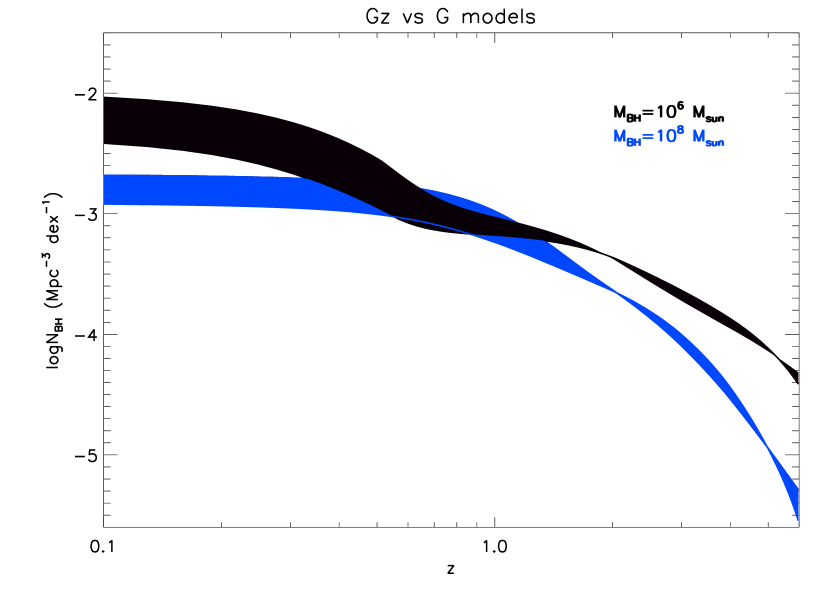
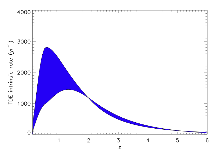
Figure 3: Upper panel: BH number density as a function of $z$ for $10^{6}$ (black shaded area) and $10^{8}$ M_⊙ (blue shaded area). Lower panel: intrinsic rate of TDEs as a function of redshift. A rate of $10^{-5}$ yr^-1 per galaxy is assumed. Most of the events are expected below $z\sim 2$.

We now need to generalize our prototypical lightcurve to a generic TDE. The main uncertainty is how the flux scales with black hole and stellar masses. A first possibility is to describe the jet evolution with a Blandford Mckee (thereafter “BM model”) solution, usually adopted for $\gamma$-ray burst afterglows (e.g. Metzger et al., 2012; Berger et al., 2012). Frequencies below 5 GHz are in the self-absorbed part of the synchrotron spectrum, for the whole observed duration of the event (see fig.3 in Berger et al., 2012). The observed specific luminosity in this regime ($\nu<\nu_{\rm a}<\nu_{\rm m}$) is given by the Raleigh Jeans part of the Black Body spectrum $B(\nu/\delta)\delta^{3}\propto k_{\rm b}T(\nu/\delta)^{2}\delta^{3}$ (see eq. 8), with a kinetic temperature given by $3k_{\rm b}T=m_{\rm e}c^{2}\gamma_{\rm min}$, where the minimum Lorentz factor for the shocked accelerated electrons is $\gamma_{\rm min}\propto\Gamma$. Therefore the specific radio luminosity is

$$L_{\nu}\propto B(\nu/\delta)\delta^{3}(r\theta_{j})^{2}\propto(r\Gamma)^{2},$$ (9)

where $(r\theta_{\rm j})^{2}$ is the emitting area, and we are assuming $\Gamma^{-1}\lower 2.15277pt\hbox{$\;\buildrel>\over{\sim}\;$}\theta_{\rm j}$. In the blast wave modelling of J1644, the external medium swept up by the jet is better described by a power-law density decay that goes as $r^{-2}$, rather than a constant density environment (Zauderer et al., 2011). This implies $\Gamma\propto E_{\rm j}^{1/4}$ and $r\propto E_{\rm j}^{1/2}$, where $E_{\rm j}\approx L_{\rm j,p}t_{\rm min}\propto m_{*}$ is the total jet energy. Therefore eq. 9 becomes, $L_{\nu}\propto(L_{\rm j,p}t_{\rm min})^{3/2}\propto m_{*}^{3/2}$, where there is no dependence on the black hole mass, but only on the stellar mass.

The simple blast wave solution, however, does not describe the whole evolution of the radio spectrum (Berger et al., 2012). Therefore, we also consider a simpler approach. In line with our treatment of the X-ray flux, we may assume that the radio luminosity is proportional to the jet peak luminosity $L_{\nu}\propto L_{\rm j,p}\propto M^{-1/2}m_{*}^{1/2}$, rather than to its total energy, (see the X-ray analogous, eq.6, which bears the same mass dependencies). As an extra motivation, this prescription may be justified in the context of the “magnetically arrested” jet model (e.g. Narayan et  al., 2003). We will call this prescription “the Mass Dependent Luminosity” model (thereafter MDL model).

The scaling of the peak flux for sources at different redshift, with different black hole and stellar masses (but at the same observed time $\tau$ from the beginning of the event) would be

$$F_{\nu}(\nu_{\rm a},\tau)=F_{\nu,sw}(\nu_{\rm a,sw},\tau_{\rm sw})\times m_{*,1}^{3/2}\left(\frac{1+z}{1+z_{\rm sw}}\right)\left(\frac{D_{\rm sw}}{D}\right)^{2},$$ (10)

for the BM solution and

$$F_{\nu}(\nu_{\rm a},\tau)=F_{\nu,sw}(\nu_{\rm a,sw},\tau_{\rm sw})\times M_{6}^{-1/2}{m_{*,1}^{1/2}}\,\left(\frac{1+z}{1+z_{\rm sw}}\right)\left(\frac{D_{\rm sw}}{D}\right)^{2},$$ (11)

for our second approach. The equivalent delay at which we need to calculate the flux of Sw J1644 is $\tau_{\rm ws}\equiv\tau\frac{1+z_{\rm sw}}{(1+z)}$.

The characteristic frequencies need to be redshifted according to

$$\nu_{\rm a}(\tau)=\nu_{\rm a,sw}(\tau_{\rm sw})\left(\frac{1+z}{1+z_{\rm sw}}\right)^{-1},$$

and

$$\nu_{\rm m}(\tau)=\nu_{\rm m,sw}(\tau_{\rm sw})\left(\frac{1+z}{1+z_{\rm sw}}\right)^{-1}.$$

In all cases, the flux $F_{\nu,sw}(\nu_{\rm a,sw},\tau_{\rm sw})$ and the characteristic frequencies at any time $\tau_{\rm sw}$ are obtained by linearly interpolating the available data. For $\tau_{\rm sw}<8$ day we extrapolate the radio light curve to earlier epochs.

3 Black hole mass functions

The mass distribution of black holes as a function of redshift is an essential ingredient to calculate TDE rates. Since black holes grow mainly by efficient accretion (Soltan, 1982), one can calculate these functions using the mass continuity equation, given a radiation efficiency and distribution of Eddington ratios. In this paper, we use the results from Shankar et al. (2013). In particular, we consider the two accretion models which yield the largest and the lowest black hole comoving number density $\phi(M,z)$, and are still consistent with the quasar bolometric luminosity functions and the local black hole mass function (models labeled $G$ and $G(z)$ in Shankar et al., 2013). In this way, we can estimate the uncertainty due to the black hole mass distribution of our expected TDE rates. In Figure 3 upper panel, we show the mass distribution functions and their uncertainty strips as a function of redshift, for $M=10^{6}M_{\sun}$ and $M=10^{8}M_{\sun}$ black holes. In Figure 3, instead, we show the “intrinsic” TDE rate as a function of redshift,

$$R(z)=\int_{M_{\rm min}}^{M_{\rm max}}\phi(M,z)V(z)N_{\rm tde}dM,$$ (12)

where we denote with $V(z)$ the comoving cosmological volume. $N_{\rm tde}=10^{-5}$ yr^-1 is our fiducial TDE rate per galaxy: this value is in the range of theoretical expectations (Merritt, 2013) and observational claims (Donley et  al., 2002; Gezari  et  al., 2009; Van Velzen et al., 2011).

The minimum black hole mass (here and thereafter in our calculations) is $M_{\rm min}=10^{6}M_{\sun}$, as just a few SMBHs have been observed with a lower mass.

4 Monte Carlo calculations

Assuming the X-ray and radio modelling described in §2, we perform Monte Carlo simulations (MCs) to derive the number of jetted TDEs to be detected per year, for given flux limit and sky coverage.

Beside the BH mass, the main ingredients of our MCs are the trigger lag time, $\tau$, and the mass of the disrupted stars, $m_{*}$. The former is randomly extracted from a uniform distribution between 0 and 1 yr. The latter follows a Kroupa Initial Mass Function, (IMF Kroupa, 2001),

$$f(m)\propto\left\{\begin{array}[]{lll}m^{-0.3},&\,\;0.01\leq m_{*}\leq 0.08,\\ m^{-1.3},&\,\;0.08\leq m_{*}\leq 0.5,\\ m^{-2.3},&\,\;m_{*}>0.5.\end{array}\right.$$ (13)

In fact, for each black hole mass, the minimum stellar mass is set by the requirement that the tidal radius should be greater than the last stable orbit (we assume a non-spinning BH). This requirement implies that $m_{\rm*min}=\max[0.01,0.045M_{6}]$. Note that for $M=10^{8}M_{\odot}$, the minimum mass is $m_{\rm*min}=4.5M_{\odot}$. Therefore, events associated with high BH masses are suppressed in numbers by the steepness of the IMF, as only $0.4\%$ of all stars have $m_{*}>8$. However, they are in average brighter, because the average $m_{*}$ is larger.

In our simulation, we start by considering the intrinsic rate $R(z)$ (eq. 12) properly modified by accounting for the relativistic beaming, which results in a reduction by a factor of $2\pi\Gamma^{-2}/(4\pi)=1/(2\Gamma^{2})$: this is the fraction of solid angle subtended by the emission, when considering a two sided jet. Our fiducial value for the jet Lorentz factor is $\Gamma=2$, as inferred by radio observations ($\Gamma\approx 2$, Zauderer et al., 2013; Berger et al., 2012). If the jet decelerates, this value has to be intended as an average one, over the observation period. However, we note that this is a geometrical scaling factor and our results may be easily re-scaled by assuming different values of the jet bulk Lorentz factor. In addition, $R(z)$ is scaled for the fraction of the sky surveyed by the assumed instrument. In the calculation of $R(z)$ we have adopted both $G$ and $G(z)$ models in order to account for the systematic uncertainties in the mass function modellings. The number of trials in MCs is properly fixed by requiring a high statistics level in each mass and redshift bin (typically $\geq 10^{4}$).

5 Results

In this section, we first validate separately our emission models for X-ray and radio light curves, by comparing our predicted rates with current instruments and survey results. In fact, we find that current data do not put strong constraints on our modelling, as we will explain in the following. Future data have instead a greater potential. In the SKA era, we propose that a strategy where radio will be triggering X-ray facilities can allow us not only to detect but also to identify and investigate jetted TDEs in a multi-wavelength fashion. In the following, if not otherwise mentioned, our results are derived adopting $\Gamma=2$.

5.1 Comparison with current surveys

5.1.1 Hard X-rays

So far, only two jetted TDE candidates have been detected by BAT, implying an observed rate of $\sim 0.3$ yr^-1.

Since BAT is not operating in survey mode, it is not straightforward to compare observations with our predictions, i.e. it is difficult to chose sky coverage and detection limit, because they are not univocally determined. The two TDE candidates were detected in two different modes: Sw J1644 was triggered onboard, while Sw J2058 was discovered by stacking 4-day integration images (Krimm et al., 2011; Cenko et al., 2012). In both modes, it is hard to define a survey flux limit, the key ingredient of our MCs. Indeed, Swift has over 500 onboard trigger criteria in different modes which makes the use of a flux limit survey a rather simplified approach. The same applies to possible discoveries of fainter TDEs with longer integration times, by applying the image mosaics technique (Krimm et al., 2013). These have to be promptly followed-up by XRT for their identification: monitor the soft X-ray emission and then measure the characteristic temporal slope of TDEs. In this way, a further efficiency accounting for any reason preventing XRT to monitor the event has to be included in our rate calculations (e.g., the stochastic nature of the Swift pointing plan, the target visibility and the mission schedule; Krimm, private communication). Such an efficiency is hard to quantify and any assumption would be arbitrary and would bias our discussion on the comparison between the predicted and observed rates. In addition to that, our soft X-ray modelling assumes a total disruption of the star (see §2), while the Sw J2058 emission seems to be consistent with a partial disruption. For both of these reasons, we focus on detections triggered onboard, although with due caveats. In fact, any reliable prediction based on on-board triggers would require complex simulations as done by (Lien et al., 2014) for GRB rates. We therefore set to achieve a less ambitious aim at predicting indicative rates, which should be considered most likely as upper limits. Specifically, we adopt the BAT daily sky coverage reported in (Krimm et al., 2013) and fix a unique “survey” flux limit to be consistent with the detection of the Sw J1644. We detail the procedure in the following.

Sw J1644 was detected with an on-board BAT image trigger (Cummings et al., 2011). In this trigger mode, we assume a flux limit of $2.5\times 10^{-9}$ erg cm^-2 s^-1 in the $15-150$ keV band, which is consistent with the faint tail of the observed GRB rate (Lien et al., 2014) and the detection of Sw J1644 (Burrows et al., 2011). We adopt a daily sky coverage of 85% (Krimm et al., 2013) and apply an efficiency of $\sim 90\%$, for the fraction of the BAT survey time (Lien et al., 2014) resulting from trigger deadtimes (e.g. due the passage through the South Atlantic Anomaly).

The detection rate is estimated by performing a large set of MCs as described in sections 2.2 and 4. In eq.5, we use a radiation efficiency of $\sim 0.3$ (Burrows et al., 2011). For each event, we compare the flux at the trigger time $\tau$ with our flux threshold. We obtain a TDE rate of $\approx 10-20$ events yr^-1 (see Table 1). The rate distribution with redshift extends up to $z_{\rm max}\approx 0.32$ and peaks at $z\approx 0.2$. The peak value ranges between $1-5$ yr^-1 (see Table 1). The peak of the corresponding BH mass distribution is at $10^{6}M_{\rm\odot}$ and contains $\sim 23\%$ of all events.

Given our predicted mass and $z$ distributions for the observed TDEs, an event like Sw J1644 has a chance probability which is a factor of $\sim 10$ lower than that of an event at the peak rate. Therefore, it is not an unlikely event, but a lower redshift object would have had a higher probability. At this point, it is unclear to us if this result is more due to our simplified treatment of the BAT trigger, to our assumption of a constant jet luminosity for a given BH and stellar mass. Both are very likely to have a role. But since we can not trust at this level our trigger modelling and the paucity of detected events does not constrain a possible luminosity function, we do not attempt here to modify our X-ray model to fit this observed distribution. When more events will be identified, our procedure can be refined to account for a TDE variety. A comparison with future, easier to model, surveys (see Sec. 5.2.1) will also help constructing a more robust emission model.

Interesting, these rates are actually up to two order of magnitude higher than that (0.3 yr^-1) derived from BAT observations, but a key role is played by the low value of $\Gamma$ considered. We will elaborate on this point in section 6.1.

5.1.2 Radio surveys at 1.4 GHz

We compare our predictions with constraints on the jetted TDE rate derived from current radio surveys (Bower, 2011). In the following radio estimates, we will require a 5-$\sigma$ flux limit to claim detection.

We first consider the combined catalogs of VLA First and NVSS at 1.4 GHz. The combined sky coverage is 0.19 sr with a flux limit of 6 mJy at 1.4 GHz. The analysis of these catalogs didn’t yield any TDE candidate.

To derive our predictions, we adopt the radio modelling described in section 2.3, and for each event (i.e. for each set of $\tau$, black hole and stellar mass, and redshift), we calculate the average flux over a period of one day from the trigger. This is compared with a 6 mJy flux threshold. Rescaling our all sky results for the catalogue sky coverage, we obtain an observed rate that even in the most favorable case ( $\sim 0.3$ yr^-1 using BM model, eq.10) is consistent with Bower (2011) and Frail et al. (2012) results. To strengthen this conclusion, we note that our assumption of a 6 mJy threshold per day combined with a sky coverage of 0.19 sr may be considered already rather optimistic, since both values are referred to a 1 yr single epoch.

In the near future, the VLA Stripe 82 survey may constrain jetted TDE models thanks to the improved sensitivity (50 $\mu$Jy rms) at 1.4 GHz over a FoV of 90 deg² (Hodge et al., 2013). By assuming a 5-$\sigma$ threshold of 0.25 mJy, our modelling predicts a number of a few objects to be detected per year. Significant advances in TDE detections are expected to come from on-going wide radio surveys at both low (see e.g. MWA and LOFAR) and high radio frequencies (e.g. ASKAP and VLASS). Since our radio modelling was constrained by observations at higher ($>1.4$ GHz) radio frequencies (as discussed in §2.3), we focus here on ASKAP and VLASS. The Variable and Slow Transient (VAST) project on ASKAP envisages a sky coverage of $10^{4}$ deg² reaching a sensitivity of $0.5~{}\rm mJy~{}\rm rms$ (VAST wide) with a daily cadence (Murphy et al., 2013). Our predictions for VAST are in the range of a few up to $\sim 14$ TDE yr^-1, consistent with expectations from Murphy et al. (2013). For comparison, Frail et al. (2012) obtain a value of $\sim 82$ yr^-1 by considering longer integration time ($\sim$ ten days). In the case of the VLA Sky Survey (Hallinan et al., 2013, VLASS), we consider a sky coverage of $10^{3}$ $\rm deg^{2}$ with $\sim 3$ week cadence at a sensitivity of $0.1~{}\rm mJy~{}\rm rms$. This set up should give a number between 2 and 6 objects to be detected per year. All sky VLASS is also foreseen and will clearly provide a larger number of TDEs, but we focus on the previous strategy because the multi-epoch survey could provide alerts for follow-up at higher energies, with a prompt identification of the transient.

5.2 Future instruments

Currently, the only two jetted TDE candidates were discovered in X-rays, where the characteristic $t^{-5/3}$ decay slope has been observed. Therefore, we first discuss the discovery potential of future X-ray surveys. We then predict the expected rate of TDEs for the SKA 1.4 GHz wide survey. Finally, we derive the properties and rate of TDEs that can be detected in radio with SKA and subsequently identified in X-rays.

5.2.1 Future X-ray surveys

The rate estimates provided in this section are based on a unique observing strategy aimed at detecting and providing a first identification of the transient as a TDE. We assume that a given fraction of the sky is covered in 1 day at a flux threshold defined by the requirement to follow the typical TDE decay over 4 lightcurve bins, each with $\rm S/N\geq 5$. This is obtained by starting from the 5-$\sigma$ flux limit of each survey, then tracing back the $t^{-5/3}$ decay in order to obtain the flux over the 4 time bins and then compute the average flux over that period. This average flux defines the identification flux threshold. We will give values for both $\Gamma=2$ and $\Gamma=20$ and we will justify this choice and elaborate on the comparison in section 6.

The all sky survey mission eRosita (Merloni et al., 2012) is expected to detect jetted TDEs, in its “hard” X-ray band ($2-10$ keV). We apply our methodology to the eRosita survey, properly re-scaling the sky coverage achieved in a 6-month scan to 1 day. We derive the identification flux threshold for our observing strategy from the $2-10$ keV 5-$\sigma$ sensitivity of $\sim 10^{-12}~{}\rm erg~{}\rm cm^{-2}~{}\rm s^{-1}$, corresponding to $\sim 250$ s exposure (Merloni et al., 2012) as foreseen for each point in the sky. We calculate the corresponding un-absorbed flux and then we extrapolate it in the energy range $1-10$ keV (used in our X-ray modelling). We predict a maximum of $\sim 15$ TDE per year to be detected up to $z\approx 2.5$, although $z_{\rm max}\approx 0.4$. The peak rate is between 0.15 and 0.5 yr^-1 at $z\approx 0.4$ and beyond $z\approx 2$, the rate is $<5\times 10^{-2}$ yr^-1. If a larger value of $\Gamma=20$ is considered, the rate decrease by two orders of magnitude (see Table 1) with a maximum total rate of $\sim 0.15$ yr^-1 and peak rate of only $4\times 10^{-3}$ yr^-1. We therefore predict both higher ($\Gamma=2$) and lower ($\Gamma=20$) rates than those previously published by Khabibullin et al. (2014, 1 object to be detected per 6-month long scan), but we definitively reach a much lower redshift ($z_{\rm max}=0.4$ vs their $z=4.5$). The same authors provide an upper limit of $\approx 150$ events per scan by considering the number of jetted TDEs to be a 1/5th of their “soft” TDE sample ($\approx 1000$). This fraction is based on results from the Rosat X-ray survey (Donley et  al., 2002). We are clearly consistent with their estimate.

The Wide Field Monitor (WFM) aboard of a LOFT-like (Feroci et al., 2012) mission will also have the capability to trigger jetted TDEs by surveying 1/3rd of the sky with a 5-$\sigma$ 1 day sensitivity of $\sim 8-9\times 10^{-11}~{}\rm erg~{}\rm cm^{-2}~{}\rm s^{-1}$ (a few mCrab) in $2-50~{}\rm keV$ energy band. We estimate tens of objects per year up to $z_{\rm max}\approx 0.6$. The peak rate is $\sim 6$ yr^-1 at $z=0.2$. These numbers imply a total rate of 0.7 yr^-1 for $\Gamma=20$ with a peak rate of only $6\times 10^{-2}$ yr^-1.

Finally, we consider Einstein Probe, which is expected to monitor $1/2$ of the entire sky in the energy range $0.5-4$ keV with a 5-$\sigma$ sensitivity of $\sim 10^{-11}{\rm erg}~{}{\rm cm^{-2}}~{}{\rm s^{-1}}$ in each point (1 ks exposed) of the sky (EP, W. Yuan private communication). In this case, MCs were adapted in order to extend our X-ray modelling to this energy range. This requires to first estimate the un-absorbed flux limit by accounting for both the Galactic and the intrinsic absorption (Burrows et al., 2011) and then calculate a proper radiation efficiency by extrapolating from the value inferred in 1-10 keV. We estimate a number between $\sim 90-240$ yr^-1 to be detected below $z_{\rm max}\approx 1$ with a peak rate of $\approx 15$ yr^-1 at $z=0.3$. In the case of $\Gamma=20$, a few objects are expected to be detected per year, with a peak rate of $\sim 0.2$ yr^-1. A summary of the actual numbers can be found in Table 1.

Inspecting the trigger time distributions (see top panel in Figure 5), we find that up to $z_{max}\sim 1$ objects are detected with almost equal probability at any delay from the explosion.

These X-ray survey rates have been obtained under the assumption of a reasonable observing strategy. A larger sample extending up to higher redshift can be obtained if longer integration times are considered, but these predictions are affected by several parameters like the trade-off between sky coverage and sensitivity. In this respect, our approach has to be considered conservative.

5.2.2 SKA as TDEs hunter

Presently, the most ambitious and revolutionary project in radio astronomy is the Square Kilometer Array (SKA Carilli & Rawlings, 2004) planned to operate in 2020. SKA, in survey mode (SKA1-Survey, Dewdney et al. (2013)), is able achieve a half sky coverage (20,000 deg²) with a 2-day cadence at a $5-\sigma$ flux limit of $90~{}\mu\rm Jy$ (Donnarumma et al., 2014; Feretti et  al., 2014). These unprecedented sky coverage and sensitivity make SKA an optimal radio transient hunter.

Differently from X-ray searches, in radio, we cannot have a first identification based on the lightcurve, since the 1.4 GHz radio emission of a TDE is not particularly different from those of other radio transients (e.g. GRB, blazars). Therefore, we consider a different strategy. In our MC simulations, we directly assume the SKA $5-\sigma$ flux limit in order to claim the detection of a transient event. The identification strategy will fully rely on the multi-frequency follow-up of the trigger event as it will be discussed at the end of this section.

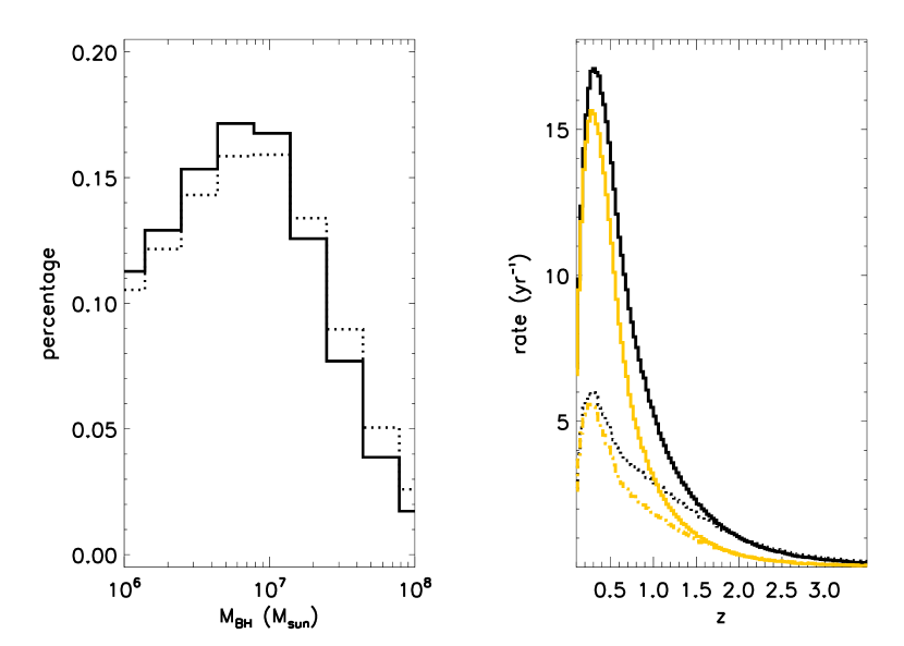
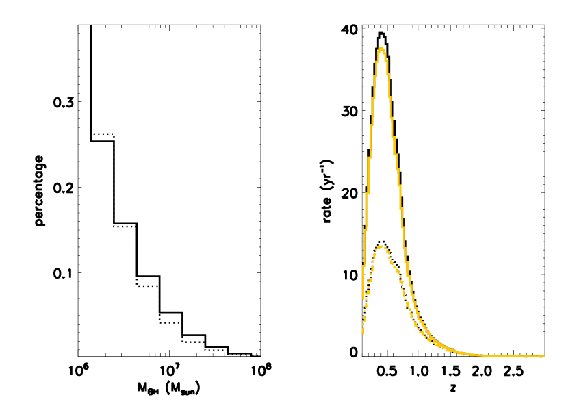
Figure 4: Rate of events predicted for SKA in wide survey mode at 1.4 GHz as a function of redshift (right panels) and their distribution as a function of BH mass (left panels), for two different black hole distribution functions (black solid line: G model black dotted line: Gz) model. Rates associated to events with BH masses lower than $10^{7}$ M_⊙ are also shown (yellow lines). Upper panels: BM model for the jet evolution; lower panels, MDL model.

We calculate the predicted average flux over 2 days from the trigger and then we compare it with the SKA flux limit. The results are shown in Figure 4. The upper panels are derived using the BM model (eq.10) for the radio lightcurve modelling, while the lower panels use the MDL model (eq.11). There, we show the distribution of the TDE rate as a function of $z$ (right panels) and their BH mass distribution (left panels) for the two BH mass functions described in §4 (black lines). The yellow lines show the subclass of events with BH masses lower than $10^{7}$ M_⊙. Both radio models produce redshift distributions peaking around $z\approx 0.4$, regardless of the BH mass function. The peak rates are roughly between $6$ and 40 yr^-1 (see also Table 1). Events with BH mass lower than $10^{7}$ $M_{\sun}$ dominate the distributions at all redshifts in the MDL model, while this only happens at $z<0.4$ in the BM model. One marked difference between the two radio lightcurve modellings is the BH mass distribution of the detected events: while BH with masses between $10^{7}-10^{8}M_{\sun}$ are equally probable in the BM model (because the flux is BH mass independent, eq.10), BHs with mass $<3\times 10^{6}$ completely dominate the observed sample in the MDL model. As a consequence, BM model distribution extends to higher redshifts ($z_{\rm max}\approx 2.5$ vs $z_{\rm max}\approx 1.7$), because BH masses larger than $10^{7}$ M_⊙ interact with higher mass stars (higher $m_{\rm*,min}$) and produce intrinsically brighter flares. This will allow us to study TDEs close to the peak of cosmic star formation.

In Table 1, we also report the total rates obtained by integrating these distributions in $z$ and M_BH. We obtain yearly rates of the order of a few to several hundreds. These results are not consistent with those that can be derived by using eq.4 in (Van Velzen et al., 2013): inserting our SKA survey parameters, we obtain thousands of events per year. This discrepancy is due to our inclusion of the stellar mass dependence, that modulates the TDE luminosity for a given BH mass: the lower $m_{*}$, the dimmer the event. In the assumption of a Kroupa IMF, the bulk of the events are caused by the disruption of stars with $m_{*}<1$, increasing the number of flares that are too dim to be detected.

With hundreds of events per year, SKA could be able to detect more TDEs than any currently planned X-ray survey. On the other hand, while X-ray surveys can catch the events soon after explosion (see EP performance in Figure 5 upper panel, for an example), SKA would not be able to cover the first week activity at any redshift and only at $(z<0.8)$ SKA will probe the first month (Figure 5, bottom panel). This result is independent on the assumed radio modelling. The explanation is simple: the observed radio flux at 1.4 GHz is initially increasing, contrary to that in the X-ray band. In this regard, detections in these two bands are complementary. However, a word of caution here is due. As mentioned before, below 10 days, we have virtually any detection in radio at any $z$. This early period coincides with the rise of the radio light curve. Although we expect this gap in detection, the exact epoch at which it occurs depends on the detailed behavior of the light curve during this undetected rise. Our extrapolation at earlier times is quite steep and we consider 10 days as an upper limit for the initial gap in detection.

So far we focused on detection of TDEs with SKA, that, depending on the observing strategy, will only be a fraction of a noticeable sample of slow radio transients. As mentioned earlier, we cannot use radio properties or variability alone to distinguish a TDE candidate from neither a slowly variable AGN or a GRB. A possibility for identification that we explore below is through quick follow-ups at higher energies, particularly in X-rays. A first pre-screening of the radio candidates could be done by cross-correlating the radio transient positions with deep AGN catalogues, expected to be provided in the near future by optical surveys (e.g. LSST) or the SKA precursors (e.g. ASKAP). However, we expect a larger degree of contamination of the TDE sample to come from transient sources such as GRBs. Since, unlike GRBs, most of TDEs should have a nuclear origin, it is mandatory to quickly identify the host galaxy. An accurate localization of the radio transient in the core of galactic nuclei, helping to assess the nuclear origin, will therefore play a major role in the screening of the radio transient sample. This means that first the host galaxy has to be found by a rapid optical follow-up and after the brighter transients could be localized by SKA with a precision of $\sim 100$ milliarcsecond (mas) essential to separate nuclear transients from other phenomena (e.g., GRB).

For details see Donnarumma et al. (2014).

5.2.3 Combining Radio and X-rays in the SKA era

X-ray follow-up will have a major role in the identification of the TDE candidate detected by SKA because of the possibility to detect the characteristic $t^{-5/3}$ decay. A possible X-ray follow-up strategy aimed at identifying and then characterizing the event consists in a fast repointing of the transient detected by SKA. We consider a 1-day delay in the X-ray repointing and require a set of X-ray observations spread over a few days in order to follow the characteristic temporal decay of the TDE. We foresee an observing strategy which is similar to the one adopted in the case of future X-ray surveys (see section 5.2.1): four observations spread over 4 days, with $S/N$ ratio $\geq 10$ in each. A high $S/N$ is required in order to characterize both the temporal and spectral behavior of the source.

For each event in the MCs, we calculate the average X-ray flux over the 4 days after the repointing and compare it with the identification flux threshold derived as explained in section 5.2.1, with the only difference of a $S/N\geq 10$ requested in each observation. Practically, $\tau$ in eq.5 has to be the radio trigger time-lag, plus an extra delay of one day for repointing, and $0\leq\Delta t\leq 3$. In this way, we derive the properties of samples of TDEs which are first detected in radio and promptly followed-up in X-rays.

In Fig. 6, we show the fraction of SKA candidates that can be identified as a function of the X-ray (1-10 keV) unabsorbed flux limit. A rapid X-ray follow-up will be able to detect a complete radio-selected sample provided that the instrument sensitivity is close to $F_{\rm lim}\lesssim 10^{-11}~{}\rm erg~{}cm^{-2}~{}s^{-1}$ in the energy. In fact, a moderate sensitivity $\sim 10^{-11}-10^{-10}~{}\rm erg~{}cm^{-2}~{}s^{-1}$ is already enough to detect equal or a larger number of events than with X-ray wide sky instruments alone. It is therefore clear that a radio trigger is a more efficient way to build up a large X-ray sample of TDEs. Rates reported in that Figure assume a fast (1 day) X-ray repointing and $F_{\rm lim}$ reached with an integration of $\sim 4$ days. Rates could be substantially different if longer integrations are needed to reach the same $F_{\rm lim}$ or in the case of longer repointing time. This is a natural consequence of the decreasing trend of the X-ray light curve.

When considering an actual follow-up strategy, the values reported in Figure 6 should be scaled by the fraction of sky accessible to the X-ray instrument considered. In general, the X-ray follow-up will provide us with a sub-sample of radio triggered TDEs, defined by the target accessibility, the repointing chance of the X-ray satellite and the sensitivity of the instruments. Since TDEs also emit in hard X-rays, a trade-off between sensitivity, sky coverage and a broad energy range is foreseen. In particular, the broader is the energy range the better the characterization of the non-thermal process and of the jet energy budget.

Future X-ray experiments like Athena (Nandra et  al., 2013) and a LOFT-like mission (Feroci et al., 2012) could offer a unique chance to follow-up and characterize SKA triggered TDEs. Moreover, if Swift were still operating in the 2020s, XRT will have a great potential in following-up the radio candidates.

Athena sensitivity lies in the saturation branch of Figure 6, which implies that the observed rate of X-ray jetted TDEs will be crucially linked to its follow-up efficiency. This is mainly influenced by the Athena sky accessibility which is of the order of $\sim 50\%$ (Athena mission proposal), resulting in a rate of TDEs of a few hundreds, with detections up to $z_{\rm max}\approx 2$ (see Table 1).

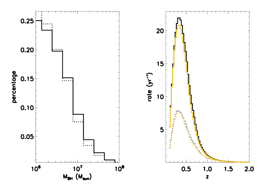
Figure 7: As Figure 4, but for radio triggered events repointed by a LOFT-like mission.

The LAD (Large Area Detector) on board of LOFT (2-50 keV) is a collimated instrument with 1 degree field of view, and a background limited sensitivity of $\geq 10^{-12}~{}\rm erg~{}\rm cm^{-2}~{}\rm s^{-1}$ in the 2-10 keV band, for a 100 ks exposure. The LOFT pointing visibility will assure a sky accessibility for these targets of $\sim 75\%$, (LOFT Yellow Book). The requirements of our strategy define a $F_{\rm lim}\sim 10^{-11}~{}\rm erg~{}\rm cm^{-2}~{}\rm s^{-1}$ in the 2-10 keV band, which was then translated in the corresponding un-absorbed value in the 1-10 keV band (the energy range adopted in our modelling). Again, we assume a 1-day repointing delay. Figure 7, shows the expected rate of jetted TDEs for a LOFT-like mission as a function of redshift (right panel) and their mass distribution (left panel). The rate distributions are calculated under the BM model (top panels) and MDL model (bottom panels) for the radio modelling. In both cases, we found that the redshift distribution extends above $z=1$ ($z_{\rm max}\approx 1.2-1.7$) (see Table 1), with most of the TDEs expected around $z\backsimeq 0.4$ (right panels). The peak rates are roughly between $\approx 4$ and 20 events per year. In the MDL model, because of the mass dependence of both the radio and X-ray luminosities, $\sim 25\%$ of all events have BHs with masses $\approx 10^{6}~{}\rm M_{\odot}$, and events with BH masses $<10^{7}~{}\rm M_{\odot}$ dominate the redshift distribution at all epochs. In the BM model, instead, the TDE rate peaks at $\approx 10^{7}~{}\rm M_{\odot}$ (see left panel in Figure 7), with lighter BHs dominating at $z\leq z_{peak}$ (yellow lines in Figure 7, right panel). The behavior at higher $z$ fully reflects the one observed in the BM radio rates (see fig. 4). In total, a LOFT-like mission should be able to detect a sub-sample of radio TDEs between $\approx 130$ and $\simeq 350$ yr^-1. Instead, very few objects per year are predicted if $\Gamma=20$. For these events, the mission broad energy band ($2-50~{}\rm keV$) should enable us to put tighter constraints on the energy budget of the X-ray component, than possible with Athena instrument.

The price to pay for detecting more X-ray TDEs with a follow-up strategy is illustrated in Figure 5 upper panel, where we compare the trigger distribution for the EP (black lines) and the LOFT radio triggered (blue lines) samples. Most of LOFT events are observed after 10 days from the beginning of the emission. In particular, high redshift $z\approx 1$events are all a couple of months old. Direct discovery of TDEs in X-rays is thus important for catching the event in its very early dynamical stages, when the jet has just formed and the disc may still be in the (largely unconstrained) super-Eddington regime.

	$R^{1}$	$R^{2}$	$z_{\rm peak}$	$R_{\rm peak}^{1}$	$R_{\rm peak}^{2}$	zmax
	yr-1	yr-1		yr-1	yr-1
Radio selected sample
SKA BM	226	468	$0.3$	6	17	$2.5$
SKA MDL	327	770	$0.4$	14	40	1.7
LOFT-like BM	128 (2.5)	305 (6.5)	$0.3$	4.5 (0.05)	13 (0.1)	1.7
LOFT-like MDL	135 (1.3)	352 (3.5)	0.4	8 (0.08)	22 (0.2)	1.2
Athena BM	113 (1)	234 (2.3)	0.3	3 (0.03)	8.5 (0.09)	$2$
Athena MDL	163 (1.6)	385 (4)	0.4	7 (0.07)	20 (0.2)	1.4
X-ray surveys
BAT3	9.5 (0.095)	26.5 (0.26)	$0.1-0.2$	1.7 (0.02)	4.6 (0.05)	0.32
eRosita	8 (0.08)	15 (0.15)	$0.4$	0.15 (0.001)	0.5 (0.005)	0.4
Einstein Probe	89 (0.9)	242 (2.4)	0.3	5.5 (0.05)	15 (0.2)	1
LOFT-like WFM	24.5 (0.2)	67 (0.7)	0.2	2.3 (0.02)	6 (0.06)	0.6

Table 1: Future Radio and X-ray surveys predictions: 1st and 2nd columns are total yearly rate (the subscripts ¹ and ² are for the $Gz$ and $G$ MFs, respectively), 3rd column redshift at the peak rate, 4th and 5th columns maximum peak rate and 6th column maximum redshift, defined as the z where the rate is 0.5. BAT³: calculation for an on-board image trigger. X-ray and Radio expected rates are derived for $\Gamma=2$. X-ray rates are also reported for $\Gamma=20$ in parenthesis.

6 Discussion

The Swift/BAT discovery of Sw J1644 opened a window on a new class of X-ray and radio transients, which are optimal targets for future radio and X-ray surveys/instruments. The study of these objects allows us to investigate the formation of transient jets in extra-galactic sources. Moreover, there is the potential to discover quiescent SMBHs in distant galaxies and constrain the SMBH mass function. In this section, we qualitatively discuss our results and what we may learn from them. Any quantitative parameter investigation (for instance with a Fisher Matrix technique) is beyond the scope of this present paper, and will be presented in a follow-up work.

6.1 Jet efficiencies and bulk Lorentz factor

So far, only two jetted TDEs have been detected, while the thermal candidates, related to the presence of an accretion disk, have been more numerous. The question then arises whether this is due to observational biases, highly collimated jets or to an intrinsic low efficiency of transient accretion disks to produce (luminous) jets.

To try and address this question, we could compare our predictions to the Swift/BAT observed rate ($\approx 0.3$ yr^-1): our lower limit ($\approx 9$ yr^-1) is a factor of 30 higher. It is tempting — and indeed it has been done in the literature — to reconcile this discrepancy by invoking a jet production efficiency of a few percent, since our calculations assume that each TDE is accompanied by a jet.

However, there are several reasons why this inference should not be drawn. First, as discussed in Section 5.1.1, it is absolutely non-trivial to describe the characteristics (e.g. flux limit and sky coverage) of an effective Swift/BAT survey. We believe that our assumptions for the trigger, together with a 100% identification efficiency gives rates that are indicative of an upper limit. Second, BAT rate predictions, unlike those of other X-ray instruments consider here, strongly depend on the modelling of the early stage variability of the X-ray lightcurve (see §2). The onboard threshold we use is very close to the flux of the upper envelope of the lightcurve. We are therefore implicitly assuming that we can always trigger an event, by catching it at its maximum. However, since the flux varies by two orders of magnitude, our choice implies again an upper limit estimate of BAT rates. Finally, even if we trust our modelling of the BAT trigger and initial X-ray variability, uncertainties in the value of $\Gamma$ can account for the discrepancy. So far, we have considered a bulk Lorentz factor of 2, since the radio measurements strongly support such a low ($\Gamma\sim 2-5$) value. However, hard X-ray observations are consistent with larger Lorentz factors ($\Gamma\leq 20$ Burrows et al., 2011), which will bring down our rates to the observed value (see Tab.1). The consequence would be that the simultaneous hard X-ray and the radio emissions need to come from different regions — as already claimed (e.g. Zauderer et al., 2011). The picture may be that while the radio emission is produced from further out, after the jet has substantially decelerated, X-rays probes regions much closer to the central engine (Bloom et al., 2011). If that was true, X-ray detections and follow-ups would be further suppressed with respect to the expected SKA performance.

Unlike the previous comparison with BAT results, our predictions of the radio rates are consistent with the upper limits derived using with the NVSS + FIRST catalog (Bower, 2011), for any $\Gamma\geq 2$. As a consequence, this comparison cannot provide us with further constraints on either $\Gamma$ or the jet efficiency. In the next future, surveys such as VLA Stripe 82, ASKAP and VLASS will give tighter constraints on jetted TDEs thanks to the improved sensitivity (50 $\mu$Jy rms, Hodge et al., 2013) of the former and the wide field of view of the latter two surveys. In this case, our radio modelling predicts a number of a few objects $\rm yr^{-1}$ (a few tens yr^-1) to be detected by assuming $\Gamma=2$. Comparing predictions with (positive) observations will thus constrain possible combinations of $\Gamma$ and jet production efficiency.

As already discussed, the optical transient surveys Pan-STARRS and LSST are expected to make significant advances in the study of TDEs. LSST will be a real breakthrough in this respect, surveying $2\times 10^{4}$ square degrees of the southern sky. Thousands of objects are expected to be discovered at $z<1$ by catching their thermal light from the accretion disc or from the non-relativistic wind in the Super-Eddington phase, surveying the same fraction of the sky every 3 days (Strubbe & Quataert, 2009; Van Velzen et  al., 2011a). However, optical extinction in galactic nuclei still introduce an observational bias in the TDEs discovery although less significant with respect to that occurring in the UV band. As suggested by (Strubbe & Quataert, 2009), infrared surveys will provide a complementary approach being the lower frequency energy range less affected by any source of obscuration.

Contrary to radio and X-ray emissions, the optical and infrared light are not expected to be relativistically beamed nor to be connected with jet emission. These features imply that a comparison between optical, X-ray and radio selected samples can help constraining both the TDE efficiency to produce jets and the relativistic Lorentz factor. This latter, when an X-ray sample is available, will help assessing the jet energy efficiency $\epsilon_{\rm j}$.

6.2 Supermassive BH masses

To understand supermassive BH cosmic growth and their connection with the host galaxy, it is necessary to have a good understanding of which mass can be found in which galaxy and, more broadly, of the SMBH mass function as a function of redshift.

The detection and light modelling of a TDE event is a unique way to constrain the mass of an otherwise quiescent BH, that is too distant to be detected by stellar dynamics. An attractive feature is that TDEs may occur in any type of galaxy, allowing for the detection of a broader range of SMBH hosts. For the lightcurve modelling, a multi-wavelength approach can yield tighter constraints on the mass, since other parameters such as the jet energy, Lorentz factor and the stellar mass need to be simultaneously determined.

A perhaps more direct measurement of the BH mass can come from very fast X-ray variability, as the quasi periodic oscillation (QPO) observed in Sw J1644 (Reis et al., 2012). The prospect for detection of QPOs in such events is quite favorable for both Athena and a LOFT-like mission. If QPOs in TDEs were associated with the Keplerian frequency at the innermost stable orbit (as discussed in Reis et al., 2012), the highest rest frame frequency should be of the order of $200s$ for a BH mass of $10^{6}~{}\rm M_{\odot}$. This QPO frequency is easily within reach of both $LOFT$-like and Athena instruments (Feretti et  al., 2014; Nandra et  al., 2013). Longer oscillations are expected for more massive BHs ($\propto\sqrt{10^{6}/\rm M_{\rm BH}}$), whose detectability could be more complicated due to satellite orbit constraints (e.g. Earth occultation, South Atlantic Anomaly). However, providing that the QPO is persistent over a long period and the source is bright enough to remain above threshold for several cycles, a direct measure of such a QPO is also possible.

An other method to constrain the mass function may be to compare our rate distributions with future SKA triggered observations. As shown by Figure 3 upper panel, there are still uncertainties in the BH mass function, which in turn affect our rate predictions (see Figure 3 lower panel, Figure 4 and Figure 7).

7 Conclusions

We have investigated the best strategies to increase the sample of the new class of TDEs, which was recently discovered by BAT. These events emitted non-thermal emission in X-ray and radio bands, probing a relativistic jet. Given the lack of statistics and of a solid theoretical framework for their non-thermal emission, we adopted a rather phenomenological approach to model their lightcurve. We fit the behavior of the best studied candidate, Sw J1644, in both radio (1.4 GHz) and X-rays (1-10 keV), and we used the classical theory of TDEs to rescale the emission for different black hole and star masses. In the radio band, we also considered, in alternative, the blast wave model, usually adopted for GRBs. We then used a Monte Carlo code to compute their expected rate as a function of redshift and black hole mass. We considered both current and future radio and X-ray surveys/instruments. Since the characteristic temporal decay of a TDE event can be observed in X-ray, an identification is claimed only when the X-ray emission can be sampled in at least 4 lightcurve bins with high signal to noise ratio, $S/N\geq 5$. When the TDE is detected in radio, we investigated a follow-up strategy for identification which required X-ray detectors to sample the lightcurve with the almost the same requirements as above (but with a $S/N\geq 10$ ). To concretely explore future possibilities, we investigated in particular the expected performance of eRosita, Einstein Probe, Athena, a LOFT-like mission and SKA operating in survey mode (SKA1-SUR).

Our major findings can be summarized as follows:

• results from current instruments (such as BAT and NVSS + FIRST catalogues) do not provide constraints on jet parameters or the jet production efficiency;

• However, to reconcile BAT predictions with observations a $\Gamma\approx 20$ may be adopted, consistently with hard X-ray observations (Burrows et al., 2011). If this were true, X-ray and radio emissions should come from two different regions, as already suggested on different bases (Zauderer et al., 2011). The predicted X-ray rates would also be suppressed by $(2/20)^{2}$ with respect to those in the radio band.

• In the near future, VLA Stripe 82 survey, VLASS and ASKAP-VAST may provide from a few to ten events yr^-1, putting some constraints on possible combinations of bulk Lorentz $\Gamma$ and jet production efficiency;

• Hundreds ($\Gamma=2$) of Sw J1644-like objects per yr are expected to be within reach of SKA1-SUR at 1.4 GHz. They can probe the distant Universe up to $z\sim 2.5$. These results differ from previous, more optimistic, predictions of thousands yr^-1 (for $\Gamma=2$ Van Velzen et al., 2011)

• Future X-ray surveys will provide a more modest sample, between several (eRosita) to a maximum of $\approx 240$ (EP) jetted events per year. With a highly collimated jet, with $\Gamma=20$, these numbers drop to a maximum of a few.

• X-ray detections can be substantially enhanced, if a prompt follow-up of SKA candidate is adopted with an instrument with flux limit $\lower 2.15277pt\hbox{$\;\buildrel<\over{\sim}\;$}10^{-11}~{}\rm erg~{}\rm cm^{-2}~{}\rm s^{-1}$ in the 1-10 keV band over 4-day timescale. With that flux limit each SKA triggered event can have in principle an X-ray counterpart (see Fig.6). A suppression factor should be adopted if the X-ray emitting region would be moving with a larger Lorentz factor.

• The sample of SKA preselected X-ray events can extend up to redshift $\sim 2$ for a X-ray instrument such as Athena and the LAD on board of a LOFT-like mission. Instead, eRosita, the WFM on LOFT and EP samples will probe a redshift range only up to $z\lower 2.15277pt\hbox{$\;\buildrel<\over{\sim}\;$}1$.

• Despite the several advantages of a radio trigger, direct X-ray detections are the only way to study the early stages ($<10$ day) of the flare (see Figure 5).

Once TDE samples in different bands have been built up, the synergy between radio, X-rays and optical can in principle constrain important physical quantities such as the jet luminosity, bulk Lorentz factor, the jet production efficiency and the black hole mass function. These findings will inform theories of jet and disc formation from sudden accretion events and, on the other hand, of SMBH cosmological evolution.

Figure 1: The X-ray (0.3-10 keV) lightcurve of J1644 as a function of time from the X-ray trigger: data (absorbed flux, circle marks taken from Publicy available XRT lightcurves) versus our modelling (solid line). After a few days, the temporal decay approaches $t^{-5/3}$.

Figure 2: The radio (1.4 GHz) light curve of SwJ 1644 as a function of time from the radio trigger (5 days after the X-ray first detection): data (circle marks) from (Berger et al., 2012; Zauderer et al., 2013) versus our modelling (solid line). While our modelling well reproduce higher radio frequencies lightcurves (see fig. 1 in (Berger et al., 2012)), it slightly underpredicts the 1.4 GHz one. In this respect our flux modelling is conservative.

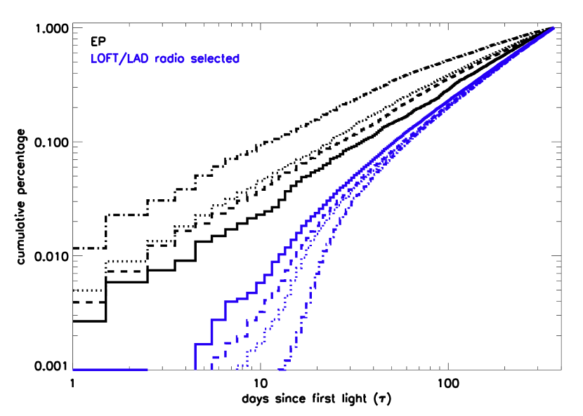
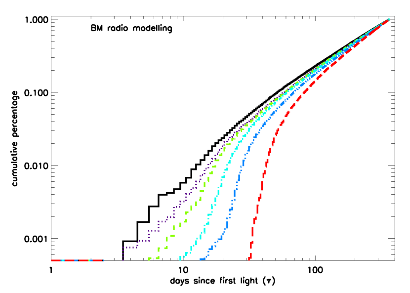
Figure 5: Cumulative distributions of delays in detecting the TDE from the explosion time, for different redshifts. Top panel: EP (black lines) and LAD follow-ups of radio triggered TDEs (blue lines). The different line styles are for $z=0.1,0.2,0.37,0.8$ from right to left for EP and viceversa for LAD. Bottom panel: the same as above but for SKA BM model and $z=0.1,0.2,0.37,0.8,1.5,3$ from left to right).

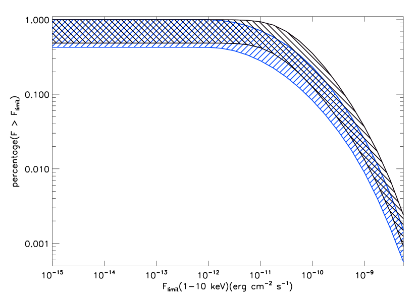
Figure 6: Fraction of X-ray TDEs that can be identified, following up a SKA trigger, as a function of flux limit (unabsorbed flux). The blue and black shaded area are obtained with eq.10 and eq.11 radio modellings, respectively. The shaded areas reflect uncertainties in BH mass functions. The figure shows that a X-ray instrument with a flux limit of $\lower 2.15277pt\hbox{$\;\buildrel<\over{\sim}\;$}10^{-11}$ in cgs units, can in principle identify any radio detected TDE. See text for details.

References

- Arcavi et al. (2014) Arcavi I. et al. 2014, Ap. J., 793, 38
- Berger et al. (2012) Berger, E., Zauderer, A., Pooley, G. G., Soderberg, A. M., Sari, R., Brunthaler, A. & Bietenholz, M. F., 2012 Ap. J.,748, 36
- Bloom et al. (2011) Bloom, J. S. et al. 2011, Science, 333, 203
- Bower (2011) Bower, G. C. 2011 ApJ, 732, L12
- Burrows et al. (2011) Burrows, D. N. et al. 2011, Nature, 476, 421
- Campana et al. (2011) Campana, S. 2011, Nature, 480, 69
- Canizzo et al. (2011) Cannizzo J. K., Troja E., & Lodato G., 2011, Ap. J., 742, 32
- Carilli & Rawlings (2004) Carilli C. L., Rawlings S., 2004, New A Rev., 48, 979
- Cenko et al. (2012) Cenko S. B., et al., 2012, Ap. J., 753, 77
- Chornock et al. (2014) Chornock R., et al., 2014, Ap. J., 780, 44
- Cummings et al. (2011) Cummings J. R., et al., 2011, GCN, 11823
- Dewdney et al. (2013) Dewdney P. E., et al., 2013, SKA1 System Baseline Design. Tech. rep., SKA Program Development, Document Number: SKA-TEL-SKO-DD-001
- Donato et al. (2014) Donato, D. et al. 2014, Ap. J.781, 59
- Donley et al. (2002) Donley, J. L. ,Brandt, W. N., Eracleous, M. & Boller,
- Donnarumma et al. (2014) Donnarumma, I. et al. 2014, “The Transient Universe with the Square Kilometre Array”, in proceedings of “Advancing Astrophysics with the Square Kilometre Array”, PoS(AASKA14)054
- Feretti et al. (2014) Feretti, L. & I. Prandoni, et al. 2014, ”Italian SKA White Book”, Eds. L. Feretti, I. Prandoni et al., INAF Press, ISBN 978-88-98985-00-5
- Feroci et al. (2012) Feroci M., et al. 2012, Experimental Astronomy, 34, 415
- Frail et al. (2012) Frail D., et al. 2012, Ap. J.747, 70
- Frank & Rees (1976) Frank, J., & Rees, M. J., 1976, MNRAS, 176, 633
- Gezari et al. (2009) Gezari S. , HeckmanT. , S. B. Cenko, M. Eracleous, K. Forster, T. S. Gonçalves, D. C. Martin, P. Morrissey, S. G. Neff, M. Seibert, D. Schiminovich, & T. K. Wyder, 2009, Ap. J.698, 1367
- Gezari et al. (2012) Gezari, S. et al. Nature, 485:217
- Granot & Sari (2002) Granot J. & Sari R., 2002, Ap. J., 568, 820
- Guillochon & Ramirez-Ruiz (2013) Guillochon, J. & Ramirez-Ruiz, E. 2013,Ap. J., 767, 25
- Hayasaki et al. (2013) Hayasaki, K. and Stone, N. and Loeb, A. 2013, Mon. Not. Roy. Astro. Soc.434, 909
- Hallinan et al. (2013) Hallinan, G. et al. 2013, VLASS White Paper
- Hills (1975) Hills, J G. 1975, Nature, 254, 295
- Holoien et al. (2014) Holoien, T. W.-S. et al. 2014, arXiv1405.1417
- Hodge et al. (2013) Hodge, J. A., Becker R. H., White R. L., Richards G. T., 2013, Ap. J., 769, 125
- Kesden (2012) Kesden, M., 2012, PhRvD, 85, 4037
- Khabibullin et al. (2014) Khabibullin I., Sazonov S., Sunyaev R., 2014, Mon. Not. Roy. Astro. Soc., 437, 327
- Kroupa (2001) Kroupa, P. 2001, Mon. Not. Roy. Astro. Soc., 322, 231
- Komossa (2002) Komossa, S., 2002, Reviews in Modern Astronomy, 15, 27
- Krimm et al. (2011) Krimm H. A. et al., 2011, Astronomer Telegrams, 3384
- Krimm et al. (2013) Krimm H. A. et al., 2013, Ap. J. Suppl., 209, 14
- Levan et al. (2011) Levan, A. J et al. 2011, Science, 333, 199
- Levan et al. (2012) Levan, A. 2012, In European Physical Journal Web of Conferences, 39, 2005
- Lien et al. (2014) Lien A., Sakamoto T., Gehrels N., Palmer D., Barthelmy S., Graziani C., Cannizzo J., 2014, Ap. J., 783, 24
- Lodato et al. (2009) Lodato G., King A. R., & Pringle J. E., 2009, Mon. Not. Roy. Astro. Soc., 392, 332
- Lodato & Rossi (2011) Lodato G. & Rossi, E. M., 2011, Mon. Not. Roy. Astro. Soc., 410, 359
- Maksym et al. (2014b) Maksym,W. P. and Lin, D. and Irwin, J. A. 2014, Ap. J. Lett., 792, 29
- Maksym et al. (2014a) Maksym,W. P. et al. 2014, AAS 223, 406
- Merloni et al. (2012) Merloni A. et al., 2012, ArXiv e-prints, arXiv1209.3114M
- Merritt (2013) Merritt D.,2013, Classical and Quantum Gravity, Volume 30, Issue 24, article id. 244005
- Metzger et al. (2012) Metzger, B. D., Giannios, D. &Mimica, P., 2012, Mon. Not. Roy. Astro. Soc., 420, 3528
- Murphy et al. (2013) Murphy, T. et al. 2013, PASA, 30, 6
- Nandra et al. (2013) Nandra P., et al., 2013, arXiv1306.2307N
- Narayan et al. (2003) Narayan R., et al., 2003, PASJ, 55, L69
- Phinney (1989) Phinney, E. S. Nature, 1989, 340, 595
- Rees (1988) Rees, M. J., 1988, Nature, 333, 523
- Reis et al. (2012) Reis, et al., 2012, Science, 337, 949
- Rossi & Begelman (2009) Rossi, E. M. & Begelman, M. C. 2009 Mon. Not. Roy. Astro. Soc.,392, 1451
- Sa̧dowski et al. (2014) Sa̧dowski A., Narayan R., McKinney J., Tchekhovskoy A., 2014, Mon. Not. Roy. Astro. Soc., 439, 503
- Sari et al. (2010) Sari, R, Kobayashi, S., & Rossi, E.M. 2010, Ap. J., 708,605
- Saxton et al. (2012) Saxton C. J., Soria R., Wu K., Kuin N. P. M., 2012, Mon. Not. Roy. Astro. Soc., 422, 1625
- Shankar et al. (2013) Shankar F., Weinberg D. H., Miralda-Escudé J., 2013, Mon. Not. Roy. Astro. Soc., 428, 421
- Soltan (1982) Soltan, A. 1982, Mon. Not. Roy. Astro. Soc., 200, 115
- Stone et al. (2012) Stone, N. and Loeb, A. 2012, Physical Review Letters 108,1302
- Stone et al. (2013) Stone, N. and Sari, R. and Loeb, A. 2013 Mon. Not. Roy. Astro. Soc., 435,1809
- Strubbe & Quataert (2009) Strubbe L. E. & Quataert, E. 2009, Mon. Not. Roy. Astro. Soc., 400, 2070
- Tchekhovskoy et al. (2013) Tchekhovskoy, A., Metzger, B. D., Giannios, D. & Kelley, L. Z., 2013, Mon. Not. Roy. Astro. Soc., accepted.
- Van Velzen et al. (2011a) van Velzen S., et al., 2011, Ap. J., 741, 73
- Van Velzen et al. (2011) van Velzen S., Frail D., Körding E., Falcke H., 2011, Mon. Not. Roy. Astro. Soc., 417, 51
- Van Velzen et al. (2013) van Velzen S., Frail D., Körding E., Falcke H., 2013, Astron. Astrophys., 552, A5
- Zauderer et al. (2013) Zauderer, B. A., Berger, E., Margutti, R., Pooley, G. G., Sari, R. , Soderberg, A. M., Brunthaler, A. & Bietenholz, M. F., 2013, Ap. J., 767, 152
- Zauderer et al. (2011) Zauderer, B. A.,et al., 2011, Nature, 476, 425