Forward-reverse EM algorithm for Markov chains: convergence and numerical analysis

Abstract.

We develop a forward-reverse EM (FREM) algorithm for estimating parameters that determine the dynamics of a discrete time Markov chain evolving through a certain measurable state space. As a key tool for the construction of the FREM method we develop forward-reverse representations for Markov chains conditioned on a certain terminal state. These representations may be considered as an extension of the earlier work Bayer and Schoenmakers (2013) on conditional diffusions. We proof almost sure convergence of our algorithm for a Markov chain model with curved exponential family structure. On the numerical side we give a complexity analysis of the forward-reverse algorithm by deriving its expected cost. Two application examples are discuss to demonstrate the scope of possible applications ranging from models based on continuous time processes to discrete time Markov chain models.

1. Introduction

The EM algorithm going back to the seminal paper Laird and Rubin (1977) is a very general method for iterative computation of maximum likelihood estimates in the setting of incomplete data. The algorithm consists of an expectation step (E-step) followed by a maximization step (M-step) which led to the name EM algorithm.

Due to its general applicability and relative simplicity it has nowadays found its way into a great number of applications. These include maximum likelihood estimates of hidden Markov models in MacDonald and Zucchini (1997), non-linear time series models in Chan and Ledolter (1995) and full information item factor models in Meng and Schilling (1996) to give just a very limited selection.

Despite the simplicity of the basic idea of the algorithm its implementation in more complex models can be rather challenging. The global maximization of the likelihood in the M-step has recently been addressed successfully (see e.g. Meng and Rubin (1993) and Liu and Rubin (1994)). On the other hand, when the expectation of the complete likelihood is not known in closed form only partial solutions have been given yet. One approach developed in Wei and Tanner (1990) uses Monte Carlo approximations of the unknown expectation and was therefore named Monte Carlo EM (MCEM) algorithm. As an alternative procedure the stochastic approximation EM algorithm was suggested in Lavielle and Moulines (1999).

In this paper we take a completely different route by using a forward-reverse algorithm (cf. Bayer and Schoenmakers (2013)) to approximate the conditional expectation of the complete data likelihood. In this respect we extend the idea from Bayer and Schoenmakers (2013) to a Markov chain setting, which is considered an interesting contribution on its own. Indeed, Markov chains are more general in a sense, since any diffusion monitored at discrete times yields canonically a Markov chain, but not every chain can be embedded (straightforwardly) into some continuous time diffusion the other way around.

The central issue is the identification of a parametric Markov chain model $(X_{n},$ $n=0,1,\ldots)$ based on incomplete data, i.e. realizations of the model, given on a typically course grid of time points, let us say $n_{1},n_{2},\ldots n_{N}.$ Let us assume that the chain runs through $\mathbb{R}^{d}$ and that the transition densities $p_{n,m}^{\theta}(x,y),$ $n\geq m,$ of the chain exist (with $p_{n,n}^{\theta}(x,y):=\delta_{x}(y)$), where the unknown parameter $\theta$ has to be determined. The log-likelihood function based on the incomplete observations $(X_{n_{1}},\ldots,X_{n_{N}})$ is then given by

(1.1) $$l(\theta,x_{n_{1}},\ldots,x_{n_{N}})=\sum_{i=0}^{N-1}\ln p_{n_{i},n_{i+1}}^{\theta}(x_{n_{i}},x_{n_{i+1}}),$$

with $X_{n_{0}}=x_{0}$ being the initial state of the chain. Then the standard method of maximum likelihood estimation would suggest to evaluate

(1.2) $$\underset{\theta}{\arg\max}\;l(\theta,X)=\underset{\theta}{\arg\max}\sum_{i=0}^{N-1}\ln p_{n_{i},n_{i+1}}^{\theta}(X_{n_{i}},X_{n_{i+1}}).$$

The problem in this approach lies in the fact that usually only the one-step transition densities $p_{n,n+1}^{\theta}(x,y)$ are explicitly known, while any multi-step density $p_{n,m}^{\theta}(x,y)$ for $m>n$ can be expressed as an $m-n-1$ fold integral of one-step densities. In particular for larger $m-n,$ these multiple integrals are numerically intractable however.

In the EM approach, we therefore consider the alternative problem

(1.3) $$\underset{\theta}{\arg\max}\sum_{i=0}^{N-1}\sum_{j=n_{i}}^{n_{i+1}-1}\mathbb{E}\ln p_{j,j+1}^{\theta}(X_{j},X_{j+1}),$$

in terms of the “missing data” $X_{n_{i}+1},...,X_{n_{i+1}-1},$ $i=0,...,N-1.$ As such, between two such consecutive time points, $n_{i}$ and $n_{i+1}$ say, the chain may be considered as a bridge process starting in realization $X_{n_{i}}$ and ending up in realization $X_{n_{i+1}}$ (under the unknown parameter $\theta$ though), and so each term in (1.3) may be considered as an expected functional of the “bridged” Markov chain starting at time $n_{i}$ in (data point) $X_{n_{i}},$ conditional on reaching (data point) $X_{n_{i+1}}$ at time $n_{i+1}.$

We will therefore develop firstly an algorithm for estimating the terms in (1.3) for a given parameter $\theta.$ This algorithm will be of forward-reverse type in the spirit of the one in Bayer and Schoenmakers (2013) developed for diffusion bridges. It should be noted here that in the last years the problem of simulating diffusion bridges has attracted much attention. Without pretending to be complete, see for example, Bladt and Sørensen (2014); Delyon and Hu (2006); Milstein and Tretyakov (2004); Stinis (2011); Stuart et al. (2004); Schauer et al. (2013).

Having the forward-reverse algorithm at hand, we may construct an approximate solution to (1.3) in a sequential way by the EM algorithm: Once a generic approximation $\theta_{m}$ is constructed after $m$ steps, one estimates

$$\theta_{m+1}:=\underset{\theta}{\arg\max}\sum_{i=0}^{N-1}\sum_{j=n_{i}}^{n_{i+1}-1}\widehat{\mathbb{E}}\ln p_{j,j+1}^{\theta}(X_{j}^{\theta_{m}},X_{j+1}^{\theta_{m}}),$$

where $X^{\theta_{m}}$ denotes the Markov bridge process under the transition law due to parameter $\theta_{m}$ and each term

$$\widehat{\mathbb{E}}\ln p_{j,j+1}^{\theta}(X_{j}^{\theta_{m}},X_{j+1}^{\theta_{m}})$$

represents a forward-reverse approximation of

$$\mathbb{E}\ln p_{j,j+1}^{\theta}(X_{j}^{\theta_{m}},X_{j+1}^{\theta_{m}})$$

as a (known) function of $\theta.$

Convergence properties of approximate EM algorithms have drawn considerable recent attention in the literature mainly driven by it’s success in earlier intractable estimation problems. An overview of existing convergence results for the MCEM algorithm can be fund in Neath (2013). Starting from a convergence result for the forward-reverse representation for Markov chains we prove almost sure convergence of the FREM sequence in the setting of curved exponential families based on techniques developed in Bayer and Schoenmakers (2013) and Fort and Moulines (2003). Essentially the only ingredient from the Markov chain model for this convergence to hold are exponential tails of the transition densities and their derivatives that are straightforward to check in many examples.

Since computational complexity is always an issue in estimation techniques that involve a simulation step, we also include a complexity analysis for the forward-reverse algorithm. We show that the algorithm achieves an expected cost of the order $O(N\log N)$ for sample size of $N$ forward-reverse trajectories.

We mention a recent application paper by Bayer, Moraes, Tempone, and Vilanova Bayer et al. (2015), which focuses on practical and implementation issues of the forward-reverse EM algorithm in the setting of Stochastic Reaction Networks (SRNs), i.e., of continuous time Markov chains with discrete, but generally infinite state space.

The structure of the paper is as follows. In Section 2 we recapitulate and adapt the concept of reversed Markov chains, initially developed in Milstein et al. (2007) using the ideas in Milstein et al. (2004) on reversed diffusions. A general stochastic representation — involving standard (unconditional) expectations only — for expected functionals of conditional Markov chains is constructed in Section 3. This representation allows for a forward reverse EM algorithm that is introduced and analyzed in Section 4. In Section 5 we proof almost sure convergence of the forward-reverse EM algorithm in the setting of curved exponential families. Implementation and Complexity of the FREM algorithm are addressed in Section 6. The paper is concluded with two application examples in Section 7 that demonstrate the wide scope of our method.

2. Recap of forward and reverse representations for Markov chains

Consider a discrete-time Markov process $(X_{n},\mathcal{F}_{n}),\ n=0,1,2,...,$ on a probability space $(\Omega,\mathcal{F},$ $\mathbb{P})$ with phase space $(S,\mathcal{S})$, henceforth called Markov chain. In general we assume that $S$ is locally compact and that $\mathcal{S}$ is the Borel $\sigma$-algebra on $S.$ For example, $S=\mathbb{R}^{d}$ or a proper subset of $\mathbb{R}^{d}.$ Let $P_{n},\ n\geq 0,$ denote the one-step transition probabilities defined by

(2.1) $$P_{n}(x,B):=\mathbb{P}(X_{n+1}\in B\ |\ X_{n}=x),\ n=0,1,2,...,\ \ x\in S,\ B\in\mathcal{S}.$$

In the case of an autonomous Markov chain all the one-step transition probabilities coincide and are equal to $P:=P_{0}=P_{1}=\cdot\cdot\cdot.$

Let $X_{m}^{n,x},$ $m\geq n,$ be a trajectory of the Markov chain which is at step $n$ in the point $x,$ i.e., $X_{n}^{n,x}=x.$ The multi-step transition probabilities $P_{n,m}$ are then defined by

$$P_{n,m}(x,B):=\mathbb{P}(X_{m}^{n,x}\in B),\ \ x\in S,\ \ B\in\mathcal{S},\ \ m\geq n.$$

Due to these definitions, $P_{n,n}(x,B)=\delta_{x}(B)=1_{B}(x)$ (Dirac measure), $P_{n}=P_{n,n+1},$ and the Chapman - Kolmogorov equation has the following form:

(2.2) $$P_{n,m}(x,B)=\int P_{n,k}(x,dy)P_{k,m}(y,B),\ \ \ \ x\in S,\ B\in\mathcal{S},\ n\leq k\leq m.$$

Let us fix $N>0$ and consider for $0\leq n\leq N$ the function

(2.3) $$u_{n}(x):=\int P_{n,N}(x,dy)f(y)=\mathbb{E}\ f(X_{N}^{n,x}),$$

where $f$ is $\mathcal{S}$-measurable and such that the mathematical expectation in (2.3) exists; for example, $f$ is bounded. By the Markov property we have for $0\leq n<N:$

$$u_{n}(x) =\mathbb{E}\ f(X_{N}^{n,x})=\mathbb{E}\ f(X_{N}^{n+1,X_{n+1}^{n,x}})$$

$$=\mathbb{E}\ \mathbb{E}^{\mathcal{F}_{n+1}}f(X_{N}^{n+1,X_{n+1}^{n,x}})=\mathbb{E}\ \mathbb{E}^{X_{n+1}^{n,x}}f(X_{N}^{n+1,X_{n+1}^{n,x}})$$

$$=\mathbb{E}\ u_{n+1}(X_{n+1}^{n,x})=\int u_{n+1}(y)P_{n}(x,dy).$$

Thus, $u_{n}(x)$ satisfies the following discrete integral Cauchy problem

(2.4) $$u_{n}(x) =\int u_{n+1}(y)P_{n}(x,dy),\ n<N,$$

(2.5) $$u_{N}(x) =f(x),$$

and (2.3) is a forward probabilistic representation of its solution. In fact, the probabilistic representation (2.3) can be used for simulating the solution of (2.4)-(2.5) by Monte Carlo. For our purpose, reverse probabilistic representations we need a somewhat more general version of the above result.

Theorem 2.1 (cf. Milstein et al. (2007)).

Let $P_{n}$ be the one-step transition density of a Markov chain $X$ as in (2.1) and let the function $f:$ $S\rightarrow\mathbb{R}$ be measurable and bounded. Let further $\varphi_{n}:$ $S\times S\rightarrow\mathbb{R}$ be a measurable and bounded functions for $n=0,1,2,...$ Then, the solution of the problem

(2.6) $$w_{n}(x) =\int w_{n+1}(z)\varphi_{n}(x,z)P_{n}(x,dz),\ \ \ n<N,$$

(2.7) $$w_{N}(x) =f(x)$$

has the following probabilistic representation:

(2.8) $$w_{n}(x)=\mathbb{E}\left[f(X_{N}^{n,x})\mathcal{X}_{N}^{n,x,1}\right],$$

where $(X,\mathcal{X})$ is an extended Markov chain in which $\mathcal{X}$ is governed by the equations

$$\mathcal{X}_{k+1}^{n,x,\gamma}=\mathcal{X}_{k}^{n,x,\gamma}\varphi_{k}(X_{k}^{n,x},X_{k+1}^{n,x}),\qquad\mathcal{X}_{n}^{n,x,\gamma}=\gamma,$$

where $n\leq k<N.$

Proof.

Note that $\mathcal{X}_{k}^{n,x,\gamma}=\gamma\mathcal{X}_{k}^{n,x,1}.$ Thus, for $n<N,$ (2.8) may be written as

$$w_{n}(x) =\mathbb{E}\left[f(X_{N}^{n+1,X_{n+1}^{n,x}})\mathcal{X}_{N}^{n+1,X_{n+1}^{n,x},\mathcal{X}_{n+1}^{n,x,1}}\right]$$

$$=\mathbb{E}\ \mathcal{X}_{n+1}^{n,x,1}\mathbb{E}^{(X_{n+1}^{n,x},\mathcal{X}_{n+1}^{n,x,1})}\left[f(X_{N}^{n+1,X_{n+1}^{n,x}})\mathcal{X}_{N}^{n+1,X_{n+1}^{n,x},1}\right]$$

$$=\mathbb{E}\ \left[\mathcal{X}_{n+1}^{n,x,1}w_{n+1}(X_{n+1}^{n,x})\right]$$

$$=\mathbb{E}\ \left[\varphi_{n}(x,X_{n+1}^{n,x})w_{n+1}(X_{n+1}^{n,x})\right]$$

$$=\int w_{n+1}(z)\varphi_{n}(x,z)P_{n}(x,dz),$$

and (2.7) is trivially fulfilled for $n=N.$ ∎

2.1. Reverse probabilistic representations

We henceforth take $\left(S,\mathcal{S}\right)=\left(\mathbb{R}^{d},\mathcal{B}(\mathbb{R}^{d})\right)$ and assume that the transition probabilities $P_{n,m}(x,dy)$ have densities $p_{n,m}(x,y)$ with respect to the Lebesgue measure on $(S,\mathcal{S}).$ We note however that without any problem one may consider more general state spaces equipped with some reference measure, and transition probabilities absolutely continuous to with respect to it. The representation (2.3) can thus be written in the form

(2.9) $$I(f):=\mathbb{E}\ f(X_{N}^{n,x})=\int p_{n,N}(x,y)f(y)dy,\text{ \ \ }0\leq n\leq N.$$

Let the initial value $\xi$ of the chain $X$ at moment $n$ be random with density $g(x).$ Consider the functional

(2.10) $$I(g,f)=\int\int g(x)p_{n,N}(x,y)f(y)dxdy=\mathbb{E}f(X_{N}^{n,\xi}).$$

Formally, by taking for $g$ a $\delta$-function we obtain (2.9) again, and by taking $f$ to be a $\delta$-function we obtain the integral

(2.11) $$J(g):=\int g(x)p_{n,N}(x,y)dx.$$

We now propose suitable (reverse) probabilistic representations for $J(g),$ where $g$ is an arbitrary test function (not necessarily a density). For this we are going to construct a class of reverse Markov chains that allow for a probabilistic representation for the solution of (2.11).

Let us fix a number $N\in\mathbb{N}$ and consider for $0\leq m<N,$ functions $\psi_{m}:$ $S\times S\rightarrow\mathbb{R}_{+}$ such that for each $m$ and $y$ the function

(2.12) $$q_{m}(y,\cdot):=\frac{p_{N-m-1}(\cdot,y)}{\psi_{m}(y,\cdot)},\text{ \ \ }0\leq m<N,$$

is a density on $S.$ For example, one could take $\psi_{m}$ independent of the second argument, and then obviously

(2.13) $$\psi_{m}(y)=\int p_{N-m-1}(z,y)dz.$$

We now introduce a “reverse” processes $(Y_{m}^{y},\mathcal{Y}_{m}^{y})_{0\leq m\leq N}$ by the system

$$\mathbb{P}(\left.Y_{m+1}^{y}\in dz^{\prime}\right|\text{ }Y_{m}^{y}=z)=q_{m}(z,z^{\prime})dz^{\prime},$$

(2.14) $$\mathcal{Y}_{m+1}^{y}=\mathcal{Y}_{m}^{y}\psi_{m}(Y_{m}^{y},Y_{m+1}^{y}),$$

$$Y_{0}^{y}:=Y_{0}^{0,y}:=y,\text{ \ \ }\mathcal{Y}_{0}^{y}:=\mathcal{Y}_{0}^{0,y,1}:=1,\text{ \ \ }0\leq m<N,$$

hence $Y^{y}$ is governed by the one-step transition probabilities $Q_{m}(z,dz^{\prime}):=$ $q_{m}(z,z^{\prime})dz^{\prime}$ (i.e. $Q_{m}$ instead of $P_{m}$).

Theorem 2.2.

For any $n,$ $0\leq n\leq N,$ (2.11) has the following probabilistic representation.

$$\int g(x)p_{n,N}(x,y)dx=\mathbb{E}\left[g(Y_{N-n}^{y})\mathcal{Y}_{N-n}^{y}\right],$$

where $g$ is an arbitrary test function (a ”density” $p_{m,m}$ has to be interpreted as a Dirac distribution or $\delta$-function).

Proof.

From the Chapman - Kolmogorov equation (2.2) we obtain straightforwardly the Chapman-Kolmogorov equation for densities,

(2.15) $$p_{n,m}(x,y)=\int p_{n,k}(x,z)p_{k,m}(z,y)dz,\ \ x,y\in S,\ n\leq k\leq m.$$

Let us now fix $n,$ $n<N$ (for $n=N$ the statement is trivial) also, and introduce the functions

(2.16) $$v_{k}(y):=\int g(x)p_{n,k}(x,y)dx,\ n\leq k\leq N.$$

From (2.15) we get

(2.17) $$v_{k}(y) =\int v_{k-1}(z)p_{k-1}(z,y)dz,\ n<k\leq N,$$

$$v_{n}(y) =g(y),$$

where $p_{k-1}:=p_{k-1,k}$ denote the one-step densities. For $\ n<k\leq N$ we now consider a “reversed” time variable $m=N+n-k$ and write with $\widetilde{v}_{m}(y):=v_{N+n-m}(y)$ and (2.12) system (2.17) in the form

(2.18) $$\widetilde{v}_{m}(y) =\int\widetilde{v}_{m+1}(z)\psi_{m-n}(y,z)q_{m-n}(y,z)dz,\ \ \ n\leq m<N,$$

$$\widetilde{v}_{N}(y) =g(y).$$

Let us write (2.18) in a slightly different form,

$$\widetilde{v}_{m}(y) =\int\widetilde{v}_{m+1}(z)\psi_{m}^{(n)}(y,z)q_{m}^{(n)}(y,z)dz,\ \ \ n\leq m<N,$$

$$\widetilde{v}_{N}(y) =g(y)$$

with $\psi_{m}^{(n)}:=\psi_{m-n}$ and $q_{m}^{(n)}:=q_{m-n}.$ Via Theorem 2.1 we next obtain a probabilistic representation of the form (2.8) for the solution of problem (2.18), hence (2.11) or $J(g).$ Indeed, by taking in Theorem 2.1 instead of $X$ a Markov chain $\left(Y_{m}^{(n),y}\right)_{n\leq m\leq N},$ where $Y^{(n),y}$ is governed by the one-step transition probabilities $Q_{m}^{(n)}(z,dz^{\prime}):=$ $q_{m}^{(n)}(z,z^{\prime})dz^{\prime},$ $n\leq m<N,$ with initial condition $Y_{n}^{(n),y}=y,$ and constructing $\left(\mathcal{Y}_{m}^{(n),y}\right)_{n\leq m\leq N}$ according to

(2.19) $$\mathcal{Y}_{m+1}^{(n),y}=\mathcal{Y}_{m}^{(n),y}\psi_{m}^{(n)}(Y_{m}^{(n),y},Y_{m+1}^{(n),y}),\qquad\mathcal{Y}_{n}^{(n),y}=1,\qquad n\leq m<N,$$

it follows by Theorem  2.1 that

(2.20) $$J(g)=\widetilde{v}_{n}(y)=v_{N}(y)=\mathbb{E}\left[g(Y_{N}^{(n),y})\mathcal{Y}_{N}^{(n),y}\right].$$

It remains to see that

$$\mathbb{E}\left[g(Y_{N}^{(n),y})\mathcal{Y}_{N}^{(n),y}\right]=\mathbb{E}\left[g(Y_{N-n}^{y})\mathcal{Y}_{N-n}^{y}\right]$$

which follows from the fact that initial values and the one step transition probabilities of the processes

$$\left(Y_{n+i}^{(n),y},\mathcal{Y}_{n+i}^{(n),y}\right)_{i=0,...,N-n}\text{ \ \ and \ \ }\left(Y_{i}^{y},\mathcal{Y}_{i}^{y}\right)_{i=0,...,N-n}$$

coincide. ∎

It should be stressed that, in contrast to a corresponding theorem in Milstein et al. (2007), Theorem 2.2 provides a family of probabilistic representations indexed by $n=1,\ldots,N,$ that involves only one common reverse process $Y^{y}.$ In Theorem 2.2 $N$ was fixed but, when different $N$ are in play, we will denote them by $Y^{y;N}.$ It turns out that this extension of the related result in Milstein et al. (2007) is crucial for deriving probabilistic representations for conditional Markov chains below (cf. Bayer and Schoenmakers (2013)).

3. Simulation of conditional expectations via forward-reverse representations

In this section we describe for a Markov Chain (2.1) an efficient procedure for estimating the final distributions of a chain $X=(X_{n})_{n=0,...,N}$ conditioned, or pinned, on a terminal state $X_{N}.$ More specifically, for some given (unconditional) process $X$ we aim at simulation of the functional

(3.1) $$\mathbb{E}\left[\left.g(X_{m_{1}},\ldots,X_{m_{r}})\right|\text{ }X_{N}=y,\,X_{0}=x\right],$$

where $0\leq m_{1}<m_{2}<\cdot\cdot\cdot<m_{r}<N$ (hence $r<N$), $g$ is an arbitrarily given suitable test function, and $x,y\in\mathbb{R}^{d}$ are given states. The procedure proposed below is in fact an extension of the method developed in Bayer and Schoenmakers (2013) to discrete time Markov chains. We note that similar techniques as in Bayer and Schoenmakers (2013) also allow us to treat the more general problem

$$\mathbb{E}\left[\left.g(X_{m_{1}},\ldots,X_{m_{r}})\right|\text{ }X_{N}\in A,\,X_{0}=x\right]$$

for suitable sets $A\subset\mathbb{R}^{d}$.

3.1. Forward-reverse representations of conditional expectations

Let us consider the problem (3.1) for fixed $x,y\in\mathbb{R}^{d}$ (i.e. $A=\{y\}$). We firstly state the following central theorem.

Theorem 3.1.

Given a grid $\mathcal{D}_{l}:=\{0\leq n^{\ast}<n_{1}<\cdot\cdot\cdot<n_{l}=:N\},$ it holds that

$$\mathbb{E}\left[f(Y_{n_{l}-n_{0}}^{y;n_{l}},Y_{n_{l}-n_{1}}^{y;n_{l}},\ldots,Y_{n_{l}-n_{l-1}}^{y;n_{l}})\mathcal{Y}_{n_{l}-n_{0}}^{y;n_{l}}\right]\\ =\int_{\mathbb{R}^{d\times L}}f(y_{0},y_{1},\ldots,y_{l-1})\prod_{i=1}^{l}p_{n_{i-1},n_{i}}(y_{i-1},y_{i})dy_{i-1}$$

with $y_{l}:=y$ and $n_{0}:=n^{\ast}.$

Proof.

Without loss of generality, we assume in this proof that the grid satisfies $n_{i}-n_{i-1}=1$, $i=1,\ldots,l$. Indeed, extend $f:\mathbb{R}^{d\times l}\to\mathbb{R}$ to a function $\tilde{f}:\mathbb{R}^{d\times(N-n^{\ast})}\to\mathbb{R}$ such that

$$\tilde{f}\left(Y_{N-n^{\ast}}^{y;N},Y_{N-n^{\ast}-1}^{y;N},\ldots,Y_{2}^{y;N},Y_{1}^{y;N}\right)=f\left(Y_{n_{l}-n_{0}}^{y;N},Y_{n_{l}-n_{1}}^{y;N},\ldots,Y_{n_{l}-n_{l-1}}^{y;N}\right).$$

Then, re-expressing the transition densities $p_{n_{i-1},n_{i}}$ in terms of the one-step transition densities $p_{i}$ using Chapman-Kolmogorov, we see that the statement of the theorem is equivalent to

(3.2) $$\mathbb{E}\left[\tilde{f}\left(Y_{N-n^{\ast}}^{y;N},Y_{N-n^{\ast}-1}^{y;N},\ldots,Y_{1}^{y;N}\right)\mathcal{Y}^{y;N}_{N-n^{\ast}}\right]\\ =\int_{\mathbb{R}^{d\times(N-n^{\ast})}}\tilde{f}\left(y_{n^{\ast}},\ldots,y_{N-1}\right)\prod_{i=n^{\ast}+1}^{N}p_{i-1}(y_{i-1},y_{i})dy_{i-1}$$

with $y_{N}\equiv y$. In fact, we shall prove that

(3.3) $$\mathbb{E}\left[f_{p}\left(Y^{y;N}_{p},\ldots,Y^{y;N}_{1}\right)\mathcal{Y}^{y;N}_{p}\right]=\int f_{p}(y_{N-p},\ldots,y_{N-1})\prod_{i=N-p+1}^{N}p_{i-1}(y_{i-1},y_{i})dy_{i-1}$$

for any $1\leq p\leq N-n^{\ast}$ for any (e.g., bounded measurable) function $f_{p}:\mathbb{R}^{d\times p}\to\mathbb{R}$. (3.3) gives the formula from the statement of the theorem for $p=N-n^{\ast}$ with $f_{N-n^{\ast}}$ being the function $\tilde{f}$ from above. We prove (3.3) by induction on $p$. For $p=1$, this boils down to Theorem 2.2 with $n=N-1$.

For the step from $p-1$ to $p$, we note that by definition

$$\mathcal{Y}_{p}^{y;N}=\mathcal{Y}_{p-1}^{y;N}\psi_{p-1}\left(Y_{p-1}^{y;N},Y_{p}^{y;N}\right),$$

with $\psi_{p-1}(y,\cdot)q_{p-1}(y,\cdot)=p_{N-(p-1)-1}(\cdot,y)=p_{N-p}(\cdot,y)$ by (2.12). Hence, we have

$$\mathbb{E}\left[f_{p}(Y_{p}^{y;N},Y_{p-1}^{y;N},\ldots,Y_{1}^{y;N})\mathcal{Y}_{p}^{y;N}\right] =\mathbb{E}\left[f_{p}(Y_{p}^{y;N},Y_{p-1}^{y;N},\ldots,Y_{1}^{y;N})\mathcal{Y}_{p-1}^{y;N}\psi_{p-1}(Y_{p-1}^{y;N},Y_{p}^{y;N})\right]$$

$$=\mathbb{E}\left[g\left(Y_{p-1}^{y;N},\ldots,Y_{1}^{y;N}\right)\mathcal{Y}^{y;N}_{p-1}\right],$$

with

$$g(z_{p-1},\ldots,z_{1}) \equiv\mathbb{E}\left[\left.f_{p}\left(Y_{p}^{y;N},Y_{p-1}^{y;N},\ldots,Y_{1}^{y;N}\right)\psi_{p-1}(Y_{p-1}^{y;N},Y_{p}^{y;N})\right|Y_{p-1}^{y;N}=z_{p-1},\ldots,Y^{y;N}_{1}=z_{1}\right]$$

$$=\int f_{p}(z,z_{p-1},\ldots,z_{1})p_{N-p}(z,z_{p-1})dz.$$

Applying the induction hypothesis for $f_{p-1}=g$, we obtain

$$\mathbb{E}\left[f_{p}(Y_{p}^{y;N},Y_{p-1}^{y;N},\ldots,Y_{1}^{y;N})\mathcal{Y}_{p}^{y;N}\right] =\mathbb{E}\left[g\left(Y_{p-1}^{y;N},\ldots,Y_{1}^{y;N}\right)\mathcal{Y}^{y;N}_{p-1}\right]$$

$$=\int g(y_{N-p+1},\ldots,y_{N-1})\prod_{i=N-p+2}^{N}p_{i-1}(y_{i-1},y_{i})dy_{i-1}$$

$$=\int f_{p}(y_{N-p},\ldots,y_{N-1})\prod_{i=N-p+1}^{N}p_{i-1}(y_{i-1},y_{i})dy_{i-1}.\qed$$

We now consider an extended integer sequence

$$0<m_{1}<\cdot\cdot\cdot<m_{k}=n^{\ast}=n_{0}<n_{1}<\cdot\cdot\cdot<n_{l}=N,$$

and a kernel $K_{\epsilon}$ of the form

$$K_{\epsilon}(u):=\epsilon^{-d}K(u/\epsilon),\quad y\in\mathbb{R}^{d},$$

with $K$ being integrable on $\mathbb{R}^{d}$ and $\int_{\mathbb{R}^{d}}K(u)du=1.$ Formally $K_{\epsilon}$ converges to the delta function $\delta_{0}$ on $\mathbb{R}^{d}$ (in distribution sense) as $\epsilon\downarrow 0.$ We then have the following stochastic representation (involving standard expectations only) for (3.1)  with $n_{i}=m_{k+i},$ $i=0,...,l=r-k+1.$

Theorem 3.2.

Let the chain $\left(Y,\mathcal{Y}\right):=\left(Y^{y;N},\mathcal{Y}^{y;N}\right)$ be given by (2.14), and the modified integer sequence $\left(\widehat{n}_{\cdot}\right)$ be defined by

(3.4) $$\widehat{n}_{i}:=n_{l}-n_{l-i},\quad i=1,\ldots,l.$$

It then holds

$$\mathbb{E}\left[\left.g(X_{m_{1}},\ldots,X_{m_{r}})\right|\ X_{m_{0}}=x,\ X_{N}=y\right]$$

$$=\mathbb{E}\left[\left.g(X_{m_{1}},\ldots,X_{m_{k-1}},X_{n^{\ast}}^{0,x},X_{n_{1}},\ldots,X_{n_{l-1}})\right|\ X_{m_{0}}=x,\,X_{N}=y\right]$$

(3.5) $$=\lim_{\epsilon\rightarrow 0}\frac{\mathbb{E}\left[g\left(X_{m_{1}}^{m_{0},x},\ldots,X_{m_{k-1}}^{m_{0},x},X_{n^{\ast}}^{m_{0},x},Y_{\widehat{n}_{l-1}}^{y;N},\ldots,Y_{\widehat{n}_{1}}^{y;N}\right)K_{\epsilon}\left(Y_{\widehat{n}_{l}}^{y;N}-X_{n^{\ast}}^{m_{0},x}\right)\mathcal{Y}_{\widehat{n}_{l}}^{y;N}\right]}{\mathbb{E}\left[K_{\epsilon}\left(Y_{\widehat{n}_{l}}^{y;N}-X_{n^{\ast}}^{m_{0},x}\right)\mathcal{Y}_{\widehat{n}_{l}}^{y;N}\right]}.$$

Proof.

The proof is analogous to the corresponding one in Bayer and Schoenmakers (2013). As a rough sketch, apply Theorem 3.1 to

$$f(X_{m_{1}}^{0,x},\ldots,X_{n^{\ast}}^{0,x},y_{0},y_{1},\ldots,y_{l-1}):=g(X_{m_{1}}^{0,x},\ldots,X_{n^{\ast}}^{0,x},y_{1},\ldots,y_{l-1})K_{\epsilon}(y_{0}-X_{n^{\ast}}^{0,x}),$$

conditional on $X_{m_{1}}^{0,x},\ldots,X_{n^{\ast}}^{0,x},$ send $\epsilon\rightarrow 0,$ and divide the result by

$$p_{0,N}(x,y)=\lim_{\epsilon\rightarrow 0}\mathbb{E}\left[K_{\epsilon}\left(Y_{\widehat{n}_{l}}-X_{n^{\ast}}\right)\mathcal{Y}_{\widehat{n}_{l}}\right].\qed$$

Forward-Reverse algorithm

Given Theorem 3.2 the corresponding forward-reverse Monte Carlo estimator for (3.5) suggests itself: Sample i.i.d. copies $X^{0,x,(1)},...,X^{0,x,(M)}$ of the process $X^{0,x}$ and, independently, i.i.d. copies $\left(Y^{y;N,(1)},\mathcal{Y}^{y;N,(\widetilde{M})}\right),...,\left(Y^{y;N,(1)},\mathcal{Y}^{y;N,(\widetilde{M})}\right)$ of the process $\left(Y^{y;N},\mathcal{Y}^{y;N}\right).$ Take for $K$ a second order kernel, take for simplicity $M=\widetilde{M},$ and choose a bandwidth $\epsilon_{M}\sim M^{-1/d}$ if $d\leq 4,$ or $\epsilon_{M}\sim M^{-2/(4+d)}$ if $d\geq 4.$ By next replacing the expectations in the numerator and denominator of (3.5) by their respective Monte Carlo estimates involving double sums, one ends up with an estimator with Root-Mean-Square error $O(M^{-1/2})$ in the case $d\leq 4$ and $O(M^{-4/(4+d)})$ in the case $d>4$ (cf. Bayer and Schoenmakers (2013) for details).

4. The forward-reverse EM algorithm

Let us now formulate the forward-reverse EM (FREM) algorithm in the setting of the missing data problem. Suppose that the parameter $\theta\in\Theta\subset\mathbb{R}^{s}$ and that the Markov chain $X=(X_{n},n\in\mathbb{N})$ has state space $\mathbb{R}^{d}$. Assuming that the transition densities $p_{n,k}$ of $X$ exist for $n,k\in\mathbb{N}$ the full-data $\log$-likelihood then reads

(4.1) $$l_{c}(\theta,x)=\sum_{i=0}^{n_{N}-1}\log p_{i,i+1}^{\theta}(x_{i},x_{i+1}),\quad x\in\mathbb{R}^{n_{N}+1}.$$

In the missing data problem only partial observations $X_{n_{0}},\ldots,X_{n_{N}}$ are available for $0=n_{0}<n_{1}<\ldots<n_{N}$ with log-likelihood function $l$ given in (1.1) that is intractable in most cases. Instead, the maximization of $l$ in $\theta$ has to be replaced by a two step iterative procedure, the EM algorithm.

E-step:

In the $m$-th step evaluate the conditional expectation of the complete data $\log$-likelihood

$$Q(\theta,\theta_{m},x):=\mathbb{E}_{\theta_{m}}[l_{c}(\theta,X_{0},\ldots,X_{n_{N}})|X_{n_{0}}=x_{n_{0}},\dots,X_{n_{N}}=x_{n_{N}}],\quad x\in\mathbb{R}^{N+1}.$$

M-step:

Update the parameter by

$$\theta_{m+1}=\arg\max_{\theta}Q(\theta,\theta_{m},X).$$

Since in many Markov chain models the E-step is intractable in this form, we propose a forward-reverse approximation for the expectation of the transition densities evaluated at the observations.

FR E-step:

Evaluate

(4.2) $$Q_{m}(\theta,\theta_{m},X):=\mathbb{E}_{\theta_{m}}^{FR}[l_{c}(\theta,X)|X_{n_{i}},i=0,\ldots,N],$$

where $\mathbb{E}_{\theta_{m}}^{FR}$ denotes a forward-reverse approximation of the conditional expectation under the parameter $\theta_{m}$.

After this FR E-step is computed the M-step remains unchanged. This FREM algorithm gives a random sequence $(\theta_{n})_{n\geq 0}$ that under certain conditions given in the next section converges to stationary points of the likelihood function. To assure a.s. boundedness of this sequence we apply a stabilization technique introduce in Chen et al. (1988).

The stable FREM algorithm

Let $K_{m}\subset\Theta$ for $m\in\mathbb{N}$ be a sequence of compact sets such that

(4.3) $$K_{m}\subsetneq K_{m+1}\quad\text{and}\quad\Theta=\bigcup_{m\in\mathbb{N}}K_{m}$$

for all $m\in\mathbb{N}$. We define the stable FREM algorithm by checking if $\theta_{m}$ after the $m$-th maximization step lies in $K_{m}$ and reseting the algorithm otherwise. Choose a starting value $\theta_{0}\in K_{0}$ and let $p_{n}$ for $n\in\mathbb{N}$, $p_{0}:=0$, count the number of resets.

stable M-step:

(4.4) $$\theta_{m+1} =\arg\max_{\theta}Q_{m}(\theta,\theta_{m},X)\text{ and }p_{n+1}=p_{n}, \quad\text{ if }\arg\max_{\theta}Q_{m}(\theta,\theta_{m},X)\in K_{m},$$

(4.5) $$\theta_{m+1} =\theta_{0}\text{ and }p_{n+1}=p_{n}+1, \quad\text{ if }\arg\max_{\theta}Q_{m}(\theta,\theta_{m},X)\notin K_{m}.$$

We will show in the next section that under weak assumption the number of resets $p_{n}$ stays a.s. finite. Our stable FREM algorithm consists now of iteratively repeating the FR E-step and the stable M-step.

5. Almost sure convergence of the FREM algorithm

In this section we prove almost sure convergence of the stable FREM algorithm under the assumption that the complete data likelihood is from a curved exponential family. Our proof is mainly based on results from Bayer and Schoenmakers (2013), Fort and Moulines (2003) and the classical framework for the EM algorithm introduced in Laird and Rubin (1977) and Lange (1995).

5.1. Model setting

Suppose that $\phi:\Theta\to\mathbb{R}$, $\psi:\Theta\to\mathbb{R}^{q}$ and $S:\mathbb{R}^{(N+1)d}\to\mathbb{R}^{q}$ are continuous functions. We make the structural assumption that the full data log-likelihood is of the form

(5.1) $$l(\theta,x_{0},\ldots,x_{N})=\phi(\theta)+\langle S(x_{0},\ldots,x_{N}),\psi(\theta)\rangle,$$

i.e. $l$ is from a curved exponential family. In order to proof convergence we need the following properties to be fulfilled that naturally hold in many popular models. In Section 6 we give several practical examples that fall into this setting.

Assumption 5.1.

1. There exists a continuous function $\bar{\theta}:\mathbb{R}^{q}\to\Theta$ such that $l(\bar{\theta}(s),s)=\sup_{\theta\in\Theta}l(\theta,s)$ for all $s\in\mathbb{R}^{(N+1)d}$.

2. The incomplete data likelihood $L$ is continuous in $\theta$, and the level sets $\{\theta\in\Theta|L(\theta,x)\geq C\}$ are compact for any $C>0$ and all $x$.

3. The conditional expectation $\mathbb{E}_{\theta}[S(X_{0},\ldots,X_{n_{N}})|X_{n_{0}}=x_{n_{0}},\dots,X_{n_{N}}=x_{n_{N}}]$ exists for all $(x_{n_{0}},\ldots,x_{n_{N}})\in\mathbb{R}^{N+1}$ and $\theta\in\Theta$ and is continuous on $\Theta$.

To simplify our notation we will neglect in the following the dependence of $l$ on $s$. Under these assumption we can separate the E- and M-step. In order to do so we define

$$g(\theta):=\mathbb{E}_{\theta}[S(X_{0},\ldots,X_{n_{N}})|X_{n_{0}}=x_{n_{0}},\dots,X_{n_{N}}=x_{n_{N}}].$$

An iteration of the EM algorithm can now be written as $\theta_{m+1}=\bar{\theta}\circ g(\theta_{m})=:T(\theta_{m})$. Let us denote by $\Gamma$ the set of stationary points of the EM algorithm, i.e.

$$\Gamma=\{\theta\in\Theta|\bar{\theta}\circ g(\theta)=\theta\}.$$

It was shown in Theorem 2 in Wu (1983) that if $\Theta$ is open, $\phi$ and $\psi$ are differentiable and Assumption 5.1 holds, then

$$\Gamma=\{\theta\in\Theta|\partial_{\theta}l(\theta)=0\},$$

such that the fixed points of the EM algorithm coincide with the stationary points of $l$. In Wu (1983) it was proved that the set $\Gamma$ contains all limit points of $(\theta_{n})$ and that $(l(\theta_{n}))$ converges to $l(\theta_{0})$ for some $\theta_{0}\in\Gamma$. In the following theorem we extend these results to the FREM algorithm. Let $d(x,A)$ be the distance between a point $x$ and a set $A$.

For the convergence of our forward-reverse based EM algorithm, we naturally also need to guarantee convergence of the corresponding forward-reverse estimators. This can be guaranteed by the following assumption (cf. also (Bayer and Schoenmakers, 2013, Section 4)).

Assumption 5.2.

1. For any multi-indices $\alpha,\beta\in\mathbb{N}_{0}^{d}$ with $|\alpha|+|\beta|\leq 2$ and any index $i$ there are constants $C_{1}=C_{1}(i,\alpha,\beta),C_{2}=C_{2}(i,\alpha,\beta)>0$ such that

   $$|\partial_{x}^{\alpha}\partial_{y}^{\beta}p_{i}(x,y)|\leq C_{1}\exp\left(-C_{2}|x-y|^{2}\right).$$

2. $S$ is twice differentiable in its arguments and both $S$ and its first and second derivatives are polynomially bounded.

Now we are ready to state as the main result of this section a general convergence theorem for the FREM algorithm.

Theorem 5.3.

Let $(K_{n})_{n\in\mathbb{N}}$ satisfy (4.3) and choose $\theta_{0}\in K_{0}$. Suppose that Assumptions 5.1 and 5.2 hold and that $l(\Gamma)$ is compact, then the stable FREM random sequence $(\theta_{n})_{n\geq 0}$ has the following properties:

1. $\lim_{n}p_{n}<\infty$ a.s. and $(\theta_{n})$ is almost surely bounded.

2. $\lim_{n}d(l(\theta_{n}),l(\Gamma))=0$ almost surely.

3. If also $l$ is $s$-times differentiable, then $\lim_{n}d(\theta_{n},\Gamma)=0$ almost surely.

Proof.

(1) Set

$$g^{FR}(\theta):=\mathbb{E}_{\theta}^{FR}[S(X_{0},\ldots,X_{n_{N}})|X_{n_{0}}=x_{n_{0}},\dots,X_{n_{N}}=x_{n_{N}}].$$

With the above notation an iteration of the FREM algorithm can be written as

$$\theta_{m+1}=\bar{\theta}(g^{FR}(\theta_{m})).$$

It was shown in Lemma 2 in Lavielle and Moulines (1999) that the incomplete data $\log$-likelihood $l$ is a natural Lyapunov function relative to $T$ and to the set of fixed points $\Gamma$. If for any $\epsilon>0$ and compact $K\subset\Theta$ we have

(5.2) $$\sum_{m}\mathbf{1}_{|l\circ\bar{\theta}(g^{FR}(\theta_{m}))-l\circ T(\theta_{m})|\mathbf{1}_{\theta_{m}\in K}\geq\epsilon}<\infty\quad\text{ a.s.},$$

then Proposition 11 in Fort and Moulines (2003) implies in our setting that $\lim\sup_{n}p_{n}<\infty$ almost surely and that $\theta_{n}$ is a compact sequence such that (1) follows. To obtain (5.2) it is sufficient by Borel-Cantelli to prove that

$$\sum_{m}P\left(|l\circ\bar{\theta}(g^{FR}(\theta_{m}))-l\circ T(\theta_{m})|\mathbf{1}_{\theta_{m}\in K}\geq\epsilon\right)<\infty.$$

Define for any $\delta>0$ an $\epsilon$-neighborhood of $K$ by

$$K_{\delta}:=\{x\in\mathbb{R}^{q}|\inf_{z\in K}|z-x|\leq\delta\}.$$

By assumption $l$ and $\bar{\theta}$ are continuous, such that for any $\delta>0$ there exists $\eta>0$ such that for any $x,y\in K_{\delta}$ we have $|l\circ\bar{\theta}(x)-l\circ\bar{\theta}(y)|\leq\epsilon$ whenever $|x-y|\leq\eta$.

Choosing now $\bar{\epsilon}=\delta\wedge\eta$ yields

$$P\left(|l\circ\bar{\theta}(g^{FR}(\theta_{m}))-l\circ T(\theta_{m})|\mathbf{1}_{\theta_{m}\in K}\geq\epsilon\right)=P\left(|l\circ\bar{\theta}(g^{FR}(\theta_{m}))-l\circ\bar{\theta}(g(\theta_{m}))|\mathbf{1}_{\theta_{m}\in K}\geq\epsilon\right)$$

$$=P\left(|l\circ\bar{\theta}(g^{FR}(\theta_{m}))-l\circ\bar{\theta}(g(\theta_{m}))|\mathbf{1}_{\theta_{m}\in K}\geq\epsilon,|g^{FR}(\theta_{m})-g(\theta_{m})|\mathbf{1}_{\theta_{m}\in K}\leq\delta\right)$$

$$+P\left(|l\circ\bar{\theta}(g^{FR}(\theta_{m}))-l\circ\bar{\theta}(g(\theta_{m}))|\mathbf{1}_{\theta_{m}\in K}\geq\epsilon,|g^{FR}(\theta_{m})-g(\theta_{m})|\mathbf{1}_{\theta_{m}\in K}\geq\delta\right)$$

$$\leq 2P\left(|g^{FR}(\theta_{m})-g(\theta_{m})|\mathbf{1}_{\theta_{m}\in K}\geq\bar{\epsilon}\right)$$

Markov’s inequality gives then

$$P\left(|l\circ\bar{\theta}(g^{FR}(\theta_{m}))-l\circ T(\theta_{m})|\mathbf{1}_{\theta_{m}\in K}\geq\epsilon\right)\leq 2\epsilon^{-k}\mathbb{E}\left[\left|g^{FR}(\theta_{m})-g(\theta_{m})\right|^{k}\mathbf{1}_{\theta_{m}\in K}\right]$$

for some $k>0$.

By (Bayer and Schoenmakers, 2013, Theorem 4.18) (see also Remark 5.4 below), we can always choose a number $N$ of samples for the forward-reverse algorithm and a corresponding bandwidth $\epsilon=\epsilon_{N}=N^{-\alpha}$ such that

$$\mathbb{E}\left[\left|g^{FR}(\theta_{m})-g(\theta_{m})\right|^{2}\mathbf{1}_{\theta_{m}\in K}\right]\leq\frac{C}{N}$$

for some constant $C$. We note that the choice of $\alpha$ depends on the dimension $d$ as well as on the order of the kernel. For instance, for $d\leq 4$ and a standard first order accurate kernel $K$, we can choose any $1/4\leq\alpha\leq 1/d$.

In any case, if we choose $N>m$ then

(5.3) $$\sum_{m}P\left(|l\circ\bar{\theta}(g^{FR}(\theta_{m}))-l\circ T(\theta_{m})|\mathbf{1}_{\theta_{m}\in K}\geq\epsilon\right)<\infty,$$

which proves (1).

To prove (2) and (3) observe that for every $K\subset\Theta$ we have

$$\lim_{m}|l(\theta_{m+1})-l\circ T(\theta_{m})|\mathbf{1}_{\theta_{m}\in K}=0\quad a.s.$$

By Borel-Cantelli it is sufficient to prove that

$$\sum_{m}P(|l(\theta_{m+1})-l\circ T(\theta_{m})|\mathbf{1}_{\theta_{m}\in K}\geq\epsilon)<\infty.$$

But since we have shown in (1) that $p_{n}$ is finite a.s., we have in the above sum that $\theta_{m+1}=\bar{\theta}(g^{FR}(\theta_{m}))$ in almost all summands. Hence, it is sufficient to show that

$$\sum_{m}P(|l(\bar{\theta}(g^{FR}(\theta_{m})))-l\circ T(\theta_{m})|\mathbf{1}_{\theta_{m}\in K}\geq\epsilon)<\infty,$$

which is nothing else than (5.3). The statement of (2) and (3) follows now from Sard’s theorem (cf. Bröckner (1975)) and Proposition 9 in Fort and Moulines (2003). ∎

Remark 5.4.

In the above convergence proof we need to rely on the convergence proof of the forward-reverse estimator when the bandwidth tends to zero and the number of simulated Monte Carlo samples tends to infinity. Such a proof is carried out for the diffusion case in (Bayer and Schoenmakers, 2013, Theorem 4.18), where also rates of convergence are given. We note that the proof only relies on the transition densities of (a discrete skeleton of) the underlying diffusion process. Hence, it immediately carries over to the present setting.

Theorem 5.3 is a general convergence statement that links the limiting points of the FREM sequence to the set of stationary points of $l$. In many concrete models the set $\Gamma$ of stationary points consists of isolated points only such that an analysis of the Hessian of $l$ gives conditions for local maxima. A more detailed discussion in this direction can be found in Lavielle and Moulines (1999) for example.

6. Implementation and complexity of the FREM algorithm

Before presenting two concrete numerical examples, we will first discuss general aspects of the implementation of the forward-reverse EM algorithm. For this purpose, let us, for simplicity, assume that the Markov chains $X$ and $(Y,\mathcal{Y})$ are time-homogeneous, i.e., that $p\equiv p_{k}$ and $q\equiv q_{k}$ do not depend on time $k$. We assume that we observe the Markov process $X$ at times $0=i_{0}<\cdots<i_{r}=N$, i.e., our data consist of the values $X_{i_{k}}=x_{i_{k}}$, $k=0,\ldots,r$. For later use, we introduce the shortcut-notation $\mathbf{x}:=(x_{i_{j}})_{j=0}^{r}$.

The law of $X$ depends on an $s$-dimensional parameter $\theta\in\mathbb{R}^{s}$, which we are trying to estimate, i.e., $p=p^{\theta}$. To this end, let

$$\ell(\theta;x_{0},\ldots,x_{N}):=\sum_{i=1}^{N}\log p^{\theta}(x_{i-1},x_{i})$$

denote the log-likelihood function for the estimation problem assuming full observation. As before, we make the structural assumption that

(6.1) $$\ell(\theta;x_{0},\ldots,x_{N})=\phi(\theta)+\sum_{i=1}^{n}S_{i}(x_{0},\ldots,x_{N})\psi_{i}(\theta).$$

For simplicity, we further assume that there are functions $S_{i}^{j}$ such that

$$S_{i}(x_{0},\ldots,x_{N})=\sum_{j=1}^{r}S^{j}_{i}(x_{i_{j-1}},\ldots,x_{i_{j}}).$$

The structural assumption (6.1) allows us to effectively evaluate the conditional expectation of the log-likelihood $\ell_{c}$ for different parameters $\theta$, without having to re-compute the conditional expectations. More precisely, recall that for a given guess $\widetilde{\theta}$ the E step of the EM algorithm consists in calculating the function

(6.2) $$\theta\mapsto Q(\theta;\widetilde{\theta},\mathbf{x}):=\mathbb{E}_{\widetilde{\theta}}\left[\left.\ell_{c}\left(\theta;X_{0},\ldots,X_{N})\right)\right|X_{i_{j}}=x_{i_{j}},\ j=0,\ldots,r\right],$$

with $\mathbb{E}_{\widetilde{\theta}}$ denoting (conditional) expectation under the parameter $\widetilde{\theta}$. Inserting the structural assumption (6.1), we immediately obtain

$$Q(\theta;\widetilde{\theta},\mathbf{x})=\phi(\theta)+\sum_{i=1}^{m}\psi_{i}(\theta)\mathbb{E}_{\widetilde{\theta}}\left[\left.S_{i}(X_{0},\ldots,X_{N})\right|X_{i_{j}}=x_{i_{j}},\ j=0,\ldots,r\right]=\phi(\theta)+\sum_{i=1}^{m}S_{i}(\theta)z_{i}^{\widetilde{\theta}}$$

with $z_{i}^{\widetilde{\theta}}:=\mathbb{E}_{\widetilde{\theta}}\left[\left.S_{i}(X_{0},\ldots,X_{N})\right|X_{i_{j}}=x_{i_{j}},\ j=0,\ldots,r\right]$, $i=1,\ldots,m$. Note that the definition of $z_{i}^{\widetilde{\theta}}$ does not depend on the free parameter $\theta$. Thus, only one (expensive) round of calculations of conditional expectations is needed for a given $\widetilde{\theta}$, producing a cheap-to-evaluate function in $\theta$, which can then be fed into any maximization algorithm.

For any given $\widetilde{\theta}$, the calculation of the numbers $z_{1}^{\widetilde{\theta}},\ldots,z_{m}^{\widetilde{\theta}}$ requires running the forward-reverse algorithm for conditional expectations. More precisely, using the Markov property we decompose

$$z_{i}^{\widetilde{\theta}}:=\mathbb{E}_{\widetilde{\theta}}\left[\left.S_{i}(X_{0},\ldots,X_{N})\right|X_{i_{j}}=x_{i_{j}},\ j=0,\ldots,r\right]\\ =\sum_{j=1}^{r}\mathbb{E}_{\widetilde{\theta}}\left[\left.S_{i}^{j}(X_{i_{j-1}},\ldots,X_{i_{j}})\right|X_{i_{j-1}}=x_{i_{j-1}},X_{i_{j}}=x_{i_{j}}\right].$$

All these conditional expectations are of the Markov-bridge type for which the forward-reverse algorithm is designed. Hence, for each iteration of the EM algorithm, we apply the forward-reverse algorithm $r$ times, one for the time-intervals $i_{j-1},\ldots,i_{j}$, $j=1,\ldots,r$, evaluating all the functionals $h_{1}^{j},\ldots,h_{m}^{j}$ at one go.

6.1. Choosing the reverse process

Recall the defining equation for the one-step transition density $q$ of the reverse process given in (2.12). For simplicity, we shall again assume that the forward and the reverse processes are time-homogeneous, implying that (2.12) can be re-expressed as

$$q(y,z)=\frac{p(z,y)}{\psi(y,z)}.$$

Notice that in this equation only $p$ is given a-priori, i.e., the user is free to choose any re-normalization $\psi$ provided that for any $y\in\mathbb{R}^{d}$ the resulting function $z\mapsto q(y,z)$ is non-negative and integrates to $1$. In particular, we can turn the equation around, choose any transition density $q$ and define

$$\psi(y,z):=\frac{p(z,y)}{q(y,z)}.$$

Note, however, that for the resulting forward-reverse process square integrability of the process $\mathcal{Y}$ is desirable. More precisely, only square integrability of the (numerator of the) complete estimator corresponding to (3.5) is required, but it seems far-fetched to hope for any cancellations giving square integrable estimators when $\mathcal{Y}$ itself is not square integrable. From a practical point of view, it therefore seems reasonable to aim for functions $\psi$ satisfying

$$\psi\approx 1$$

in the sense that $\psi$ is bounded from above by a number slightly smaller than $1$ and bounded from below by a number slightly smaller than $1$. Indeed, note that $\mathcal{Y}$ is obtained by multiplying terms of the form $\psi(Y_{n},Y_{n+1})$ along the whole trajectory of the reverse process $Y$. Hence, if $\psi$ is bounded by a large constant, $\mathcal{Y}$ could easily take extremely large values, to the extent that buffer-overflow might occur in the numerical implementation – think of multiplying $100$ numbers of order $100$. On the other hand, if $\psi$ is considerably smaller than $1$, $\mathcal{Y}$ might take very small values, which can cause problems in particular taking into account the division by the forward-reverse estimator for the transition density in the denominator of the forward-reverse estimator.

Heuristically, the following procedure seems promising.

• If $y\mapsto\int_{\mathbb{R}^{d}}p(z,y)dz$ can be computed in closed form (or so fast that one can think of a closed formula), then choose

  $$\psi(y):=\psi(y,z)=\int_{\mathbb{R}^{d}}p(z,y)dz.$$

• Otherwise, assume that we can find a non-negative (measurable) function $\widetilde{p}(z,y)$ with closed form expression for $\int_{\mathbb{R}^{d}}\widetilde{p}(z,y)dz$ such that $p(z,y)\approx\widetilde{p}(z,y)$. Then define

  $$q(y,z):=\frac{\widetilde{p}(z,y)}{\int_{\mathbb{R}^{d}}\widetilde{p}(z,y)dz},$$

  which is a density in $z$. By construction, we have

  $$\psi(y,z)=\frac{p(z,y)}{q(y,z)}=\int_{\mathbb{R}^{d}}\widetilde{p}(z,y)dz\,\frac{p(z,y)}{\widetilde{p}(z,y)},$$

  implying that we are (almost) back in the first situation.

Remark 6.1.

Even if we can, indeed, explicitly compute $\psi(y,z)=\int_{\mathbb{R}^{d}}p(z,y)dz$, there is generally no guarantee that $\mathcal{Y}$ has (non-exploding) finite second moments. However, in practice, this case seems to be much easier to control and analyze.

6.2. Complexity of the forward-reverse algorithm

We end this general discussion of the forward-reverse EM algorithm by a refined analysis of the complexity of the forward-reverse algorithm for conditional expectations as compared to Bayer and Schoenmakers (2013). We start with an auxiliary lemma concerning the maximum product of numbers of two species of balls in bins, which is an easy consequence of a result by Gonnet Gonnet (1981), see also (Sedgewick and Flajolet, 1996, Section 8.4).

Lemma 6.2.

Let $X$ be a random variable supported in a compact set $D\subset\mathbb{R}^{d}$ with a uniformly bounded density $p$. For any $K\in\mathbb{N}$ construct a partition $B_{1}^{K},\ldots,B_{K}^{K}$ of $D$ in measurable sets of equal Lebesgue measure $\lambda(B^{K}_{i})=\lambda(D)/K$, $i=1,\ldots,K$. Finally, for given $N\in\mathbb{N}$ let $X_{1},\ldots,X_{N}$ be a sequence of independent copies of $X$ and define

$$N_{k}\coloneqq\#\left\{\left.i\in\left\{1,\ldots,N\right\}\,\right|\,X_{i}\in B^{K}_{k}\right\},\quad k=1,\ldots,K.$$

For $N,K\to\infty$ such that $N=\mathcal{O}(K)$ we have the asymptotic relation

$$\mathbb{E}\left[\max_{k=1,\ldots,K}N_{k}\right]=\mathcal{O}\left(\frac{\log N}{\log\log N}\right).$$

Proof.

Let

$$p_{k}\coloneqq P\left(X\in B^{K}_{k}\right)\leq\left\lVert p\right\rVert_{\infty}/K$$

and observe that the random vector $\left(N_{1},\ldots,N_{K}\right)$ satisfies a multi-nomial distribution with parameters $K,N$ and $(p_{1},\ldots,p_{K})$.

The proof for the statement in the special case of $p_{1}=\ldots=p_{K}=1/K$ is given in Gonnet Gonnet (1981), so we only need to argue that the relation extends to the non-uniform case. To this end, let $K^{\prime}\coloneqq\left\lfloor K/\left\lVert p\right\rVert_{\infty}\right\rfloor$ and let $(M_{1},\ldots,M_{K^{\prime}})$ denote a multi-nomial random variable with parameters $N$, $K^{\prime}$ and $(1/K^{\prime},\ldots,1/K^{\prime})$. As $N=\mathcal{O}(K^{\prime})$ we have by Gonnet’s result that

$$\mathbb{E}\left[\max_{k=1,\ldots,K^{\prime}}M_{k}\right]=\mathcal{O}\left(\frac{\log N}{\log\log N}\right).$$

Moreover, it is clear that $\mathbb{E}\left[\max_{k=1,\ldots,K}N_{k}\right]\leq\mathbb{E}\left[\max_{k=1,\ldots,K^{\prime}}M_{k}\right]$ and we have proved the assertion. ∎

Theorem 6.3.

Assume that the transition densities $p$ and $q$ have compact support in $\mathbb{R}^{d}$. Moreover, assume that the kernel $K$ is supported in a ball of radius $R>0$. Then the forward-reverse algorithm for $N$ forward and reverse trajectory based on a bandwidth proportional to $N^{-1/d}$ can be implemented in such a way that its expected cost is $\mathcal{O}(N\log N)$ as $N\to\infty$.

Proof.

In order to increase the clarity of the argument, we re-write the double sum in the forward-reverse algorithm to a simpler form, which highlights the computational issues. Indeed, we are trying to compute a double sum of the form

(6.3) $$\sum_{i=1}^{N}\sum_{j=1}^{N}F_{i,j}K_{\epsilon}\left(X^{i}_{n^{\ast}}-Y^{j}_{\hat{n}_{l}}\right),$$

where $F_{i,j}$ obviously depends on the whole $i$th sample of the forward process $X$ and on the whole $j$th sample of the reverse process $(Y,\mathcal{Y})$.

We may assume that the end points $X^{i}_{n^{\ast}}$ and $Y^{j}_{\hat{n}_{l}}$ of the $N$ samples of the forward and reverse trajectories are contained in a compact set $[-L,L]^{d}$. (Indeed, the necessary re-scaling operation can obviously be done with $\mathcal{O}(N)$ operations.) In fact, for ease of notation we shall assume that the points are actually contained in $[0,1]^{d}$. We sub-divide $[0,1]^{d}$ in boxes with side-length $S\epsilon$, where $S>R$ is chosen such that $1/(S\epsilon)\in\mathbb{N}$. Note that there are $K:=(S\epsilon)^{-d}$ boxes which we order lexicographically and associate with the numbers $1,\ldots,K$ accordingly.

In the next step, we shall order the points $X^{i}_{n^{\ast}}$ and $Y^{j}_{\hat{n}_{l}}$ into these boxes. First, let us define a function $f_{1}:[0,1]^{d}\to\{1,\ldots,1/(S\epsilon)\}^{d}$ by setting

$$f_{1}(x):=\left(\lceil x_{1}/(S\epsilon)\rceil,\ldots,\lceil x_{d}/(S\epsilon)\rceil\right),$$

with $\lceil\cdot\rceil$ denoting the smallest integer larger or equal than a number. Moreover, define $f_{2}:\{1,\ldots,1/(S\epsilon)\}^{d}\to\{1,\ldots,K\}$ by

$$f_{2}(i_{1},\ldots,i_{d}):=(i_{1}-1)(S\epsilon)^{-d+1}+(i_{2}-1)(S\epsilon)^{-d+2}+\cdots+(i_{d}-1)+1.$$

Obviously, a point $x\in[0,1]^{d}$ is contained in the box number $k$ if and only if $f_{2}(f_{1}(x))=k$. Now we apply a sorting algorithm like quick-sort to both sets of points $\left(X^{1}_{n^{\ast}},\ldots,X^{N}_{n^{\ast}}\right)$ and $\left(Y^{1}_{\hat{n}_{l}},\ldots,Y^{N}_{\hat{n}_{l}}\right)$ using the ordering relation defined on $[0,1]^{d}\times[0,1]^{d}$ by

$$x<y:\iff f_{2}(f_{1}(x))<f_{2}(f_{1}(y)).$$

Sorting both sets incurs a computational cost of $\mathcal{O}(N\log N)$, so that we can now assume that the vectors $X^{i}_{n^{\ast}}$ and $Y^{i}_{\hat{n}_{l}}$ are ordered.

Notice that $K_{\epsilon}(x-y)\neq 0$ if and only if $x$ and $y$ are situated in neighboring boxes, i.e., if $\left|f_{1}(x)-f_{1}(y)\right|_{\infty}\leq 1$, where we define $\left|\alpha\right|_{\infty}:=\max_{i=1,\ldots,d}\left|\alpha_{i}\right|$ for multi-indices $\alpha$. Moreover, there are $3^{d}$ such neighboring boxes, whose indices can be easily identified, in the sense that there is a simple set-valued function $f_{3}$ which maps an index $k$ to the set of all the indices $f_{3}(k)$ of the at most $3^{d}$ neighboring boxes. Moreover, for any $k\in\{1,\ldots,K\}$ let $X^{i(k)}_{n^{\ast}}$ be the first element of the ordered sequence of $X^{i}_{n^{\ast}}$ lying in the box $k$. Likewise, let $Y^{j(k)}_{\hat{n}_{l}}$ be the first element in the ordered sequence $Y^{j}_{\hat{n}_{l}}$ lying in the box with index $k$. Note that identifying these $2K$ indices $i(1),\ldots,i(K)$ and $j(1),\ldots,j(K)$ can be achieved at computational costs of order $\mathcal{O}(K\log N)=\mathcal{O}(N\log N)$.

After all these preparations, we can finally express the double sum (6.3) as

(6.4) $$\sum_{i=1}^{N}\sum_{j=1}^{N}F_{i,j}K_{\epsilon}\left(X^{i}_{n^{\ast}}-Y^{j}_{\hat{n}_{l}}\right)=\sum_{k=1}^{K}\sum_{r\in f_{3}(k)}\sum_{i=i(k)}^{i(k+1)-1}\sum_{j=j(r)}^{j(r+1)-1}F_{i,j}K_{\epsilon}\left(X^{i}_{n^{\ast}}-Y^{j}_{\hat{n}_{l}}\right).$$

Regarding the computational complexity of the right hand side, note that we have the deterministic bounds

$$K=\mathcal{O}(N),$$

$$\left|f_{3}(k)\right|\leq 3^{d}.$$

Moreover, regarding the stochastic contributions, the expected maximum number of samples $X^{i}_{n^{\ast}}$ ($Y^{j}_{\hat{n}_{l}}$, respectively) contained in any of the boxes is bounded by $\mathcal{O}(\log N)$ by Lemma 6.2, i.e.,

$$\mathbb{E}\left[\max_{r=1,\ldots,K}(j(r+1)-j(r))\right]\mathcal{O}(\log N),$$

which then needs to be multiplied by the total number $N$ of points $X^{i}_{n^{\ast}}$ to get the complexity of the double summation step. ∎

Remark 6.4.

As becomes apparent in the proof of Theorem 6.3, the constant in front of the asymptotic complexity bound does depend exponentially on the dimension $d$.

Remark 6.5.

Notice that the box-ordering step can be omitted by maintaining a list of all the indices of trajectories whose end-points lie in every single box. The asymptotic rate of complexity of the total algorithm does not change by omitting the ordering, though.

7. Applications of the FREM algorithm

The forward reverse EM algorithm is a versatile tool for parameter estimation in dynamic stochastic models. It can be applied in discrete time Markov models, but also in the the setting of discrete observations of time-continuous Markov processes such as diffusions for example.

In this section we give examples from both worlds: we start by a discretized Ornstein-Uhlenbeck process that serves as a benchmark model, since the likelihood function can be treated analytically. Then we give an example of a partially hidden Markov model that is motivated be applications in system biology in Langrock and King (2013). Finally, we remark on limitations of the EM algorithm when the log-likelihood is not integrable and demonstrate these limitations in the context of a Cox-Ingersoll-Ross process. For a complex real data application of our method we refer the interested reader to the forthcoming companion paper Bayer et al. (2015).

7.1. Ornstein-Uhlenbeck dynamics

In this section we apply the forward-reverse EM algorithm to simulated data from a discretized Ornstein-Uhlenbeck process. The corresponding Markov chain is thus given by

(7.1) $$X_{n+1}=X_{n}+\lambda X_{n}\Delta t+\Delta W_{n+1},\quad n\geq 0$$

where $W_{n}$ are independent random variables distributed according to $N(0,\Delta t)$. The drift parameter $\lambda\in\mathbb{R}$ is unknown and we will employ the forward reverse EM algorithm to estimate it from simulated data. The Ornstein-Uhlenbeck model has the advantage that the likelihood estimator is available in closed form and we can thus compare it to the results of the EM algorithm.

In each simulation run we suppose that we have known observations

$$X_{0},X_{10\Delta t},\ldots,X_{40\Delta t}$$

for varying step size $\Delta t$ and use the EM methodology to approximate the likelihood function in between. We perform six iteration of the algorithm with increasing number of data points $N$.

In table 1 we summarize the results of two runs for the discrete Ornstein-Uhlenbeck chain. The mean and standard deviation are estimated from 1000 Monte Carlo iterations. We find that already after three steps the mean is very close to the corresponding estimate of the true MLE. This indicates a surprisingly fast convergence for this example. Note also that the approximated value of the likelihood function stabilizes extremely fast at the maximum.

$\Delta t$	N	bandwidth	mean $\hat{\lambda}$	std dev $\hat{\lambda}$	likel.	std dev likel.
0.1	2000	0.0005	0.972	0.0135	-3.402	0.00290
	8000	0.000125	1.098	0.00841	-3.383	0.00062
	32000	3.125e-05	1.132	0.00476	-3.381	0.000123
	128000	7.812e-06	1.151	0.00236	-3.381	2.783e-05
	512000	1.953e-06	1.157	0.00117	-3.381	4.745e-06
	2048000	4.882e-07	1.159	0.000581	-3.381	1.005e-06
0.05	2000	0.0005	1.160	0.0141	-3.107	0.000854
	8000	0.000125	1.247	0.00872	-3.103	9.867e-05
	32000	3.125e-05	1.253	0.00468	-3.103	1.329e-05
	128000	7.812e-06	1.265	0.00225	-3.103	3.772e-06
	512000	1.953e-06	1.265	0.00111	-3.103	6.005e-07

Table 1. Behavior of the forward-reverse EM algorithm for a discretized Ornstein-Uhlenbeck model for different step sizes $\Delta t$, initial guess $\lambda=0.5$ and true MLE $\hat{\lambda}_{\text{MLE}}=1.161$ and $1.266$, respectively.

Table 2 gives results for the same setup as in Table 1 but with initial guess $\lambda=2$ such that the forward-reverse EM algorithm converges from above to the true maximum of the likelihood function. We observe that the smaller step size $\Delta t=0.05$ results in a more accurate approximation of the likelihood and also of the true MLE. It seems that the step size has crucial influence on the convergence rate of the algorithm, since for $\Delta t=0.05$ the likelihood stabilizes already from the second iteration.

$\Delta t$	N	bandwidth	mean $\hat{\lambda}$	std dev $\hat{\lambda}$	likel.	std dev likel.
0.1	2000	0.0005	1.554	0.0353	-3.457	0.0134
	8000	0.000125	1.312	0.0127	-3.393	0.00221
	32000	3.125e-05	1.217	0.00544	-3.382	0.000351
	128000	7.812e-06	1.185	0.00245	-3.381	5.817e-05
	512000	1.953e-06	1.168	0.00121	-3.381	1.227e-05
0.05	2000	0.0005	1.390	0.0248	-3.108	0.00238
	8000	0.000125	1.289	0.00925	-3.103	0.000130
	32000	3.125e-05	1.261	0.00471	-3.103	1.451e-05
	128000	7.812e-06	1.266	0.00221	-3.103	2.538e-06
	512000	1.953e-06	1.266	0.00113	-3.103	5.855e-07

Table 2. Behavior of the forward-reverse EM algorithm for a discretized Ornstein-Uhlenbeck model for different step sizes $\Delta t$, initial guess $\lambda=2$ and true MLE $\hat{\lambda}_{\text{MLE}}=1.161$ and $1.266$, respectively.

In Figure 1 the empirical distribution of 1000 estimates for $\lambda$ is plotted. The initial value was $0.5$ and the true maximum of the likelihood function is at $1.161$. The step size between observations was chosen to be $\Delta t=0.1$. The histogram on the left shows the estimates after only one iteration and on the right the estimates were obtained from five iterations of the forward-reverse EM algorithm.

Figure 2 depicts the distribution of 1000 Monte Carlo samples of the likelihood values that led to the estimates in Figure 1. It is interesting to see that after one iteration of the algorithm the likelihood values are approximately bell shaped (left histogram) whereas after five iterations the distributions becomes more and more one-sided as would be expected, since the EM algorithm only increase the likelihood from step to step towards the maximum.

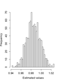
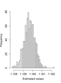
Figure 1. Empirical distribution of 1000 estimates after one iteration (right) and after five iteration (left) of the forward-reverse EM algorithm.

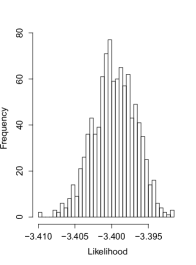
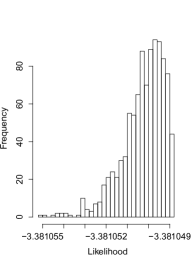
Figure 2. Empirical distribution of the likelihood values of 1000 Monte Carlo samples after one iteration (right) and after five iteration (left) of the forward-reverse EM algorithm.

Figure 3 shows the convergence of the forward reverse EM algorithm when the number of iterations increases. We find that already after 4 iterations the estimate is very close to the true MLE for $\lambda$. After six iterations the algorithm has almost perfectly stabilized at the value of the true MLE $\lambda=1.16$.

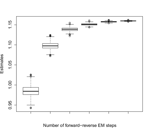
Figure 3. Convergence of the forward-reverse EM algorithm from one to six iterations for each 1000 estimates of $\lambda$. The value of the true MLE is $\hat{\lambda}=1.161$.

7.2. Hidden Markov models

Our forward reverse EM algorithm can also be applied in the context of hidden Markov models (HMM). A typical HMM consists of observed state process and a hidden (i.e. unobserved) Markov chain that models the internal regime switching of the state process (see for example MacDonald and Zucchini (1997) for a general introduction). When for the hidden process only some values can be observed we speak of a partially HMM.

Recently, partially HMMs have been applied with some success in the modeling of ecological systems to understand the relation between animal populations and environmental parameters in a dynamical setting. The example considered here is a partially hidden Markov model and is inspired by applications in modeling mark-recapture-recovery data as discussed in Langrock and King (2013) for example. In mark-recapture-recovery studies every individual of a population is marked by some tag or ring that uniquely identifies the individual and some properties of interest are measured (e.g. weight, age etc). In subsequent surveys each individual is either recaptured such that the measurements could be taken again or if it can not be recaptured this will be recorded as a missing data point. Hence, we obtain a sequence of data with missing values that leads naturally to a partially HMM.

Let us consider a two-dimensional Markov chain $X_{n}=(X_{n}^{1},X_{n}^{2})$. For the first component $N$ observations $X_{0}^{1},\ldots,X_{N}^{1}$ are given, whereas the second component $X^{2}$ is only observed partially after each $k\in\{1,\ldots,N\}$ time steps, i.e.

$$X_{0}^{2},X_{k}^{2},X_{2k}^{2},\ldots,X_{\lfloor\frac{N}{k}\rfloor k}^{2}$$

are known. Suppose that the one-step transition probabilities are normal distributions:

$$\mathcal{L}(X_{n+1}|X_{n})=N(\mu^{\theta}(X_{n}),\Sigma),$$

with mean given by $\mu^{\theta}(x)=\theta+x^{2}$ for an unknown parameter $\theta\in\mathbb{R}^{2}$. The covariance matrix $\Sigma\in\mathbb{R}^{2\times 2}$ is assumed to be constant.

In this setup the $\log$-likelihood function based on full observations $X$ is given by

$$l_{c}(\theta,X_{0},\ldots,X_{N})=1-2\pi\det(\Sigma)^{1/2}-\frac{1}{2}\sum_{l=1}^{N}Y_{l}^{\theta}.$$

where

$$Y_{l}^{\theta}=\left(X_{l}-\mu^{\theta}(X_{l-1})\right)^{\top}\Omega\left(X_{l}-\mu^{\theta}(X_{l-1})\right)$$

with precision matrix $\Omega=(\omega_{ij}):=\Sigma^{-1}$. In coordinates we thus have

$$Y_{l}^{\theta}=\omega_{11}(U_{l,1})^{2}+(2\omega_{12})U_{l,1}U_{l,2}+\omega{22}U_{l,2}^{2},$$

where $U_{l,i}:=X_{l}^{i}-\theta_{i}-(X_{l-1}^{i})^{2}$. Calculating the score function gives therefore

$$\frac{\partial l_{c}}{\partial\theta_{1}}=-\frac{1}{2}\sum_{l=1}^{N}\omega_{11}\left(2(X_{l}^{1})^{2}+\theta^{1}+2(X_{l-1}^{1})^{2}\right)+2\omega_{12}\left(\theta^{2}-X_{l}^{2}+(X_{l-1}^{2})^{2}\right)$$

and

$$\frac{\partial l_{c}}{\partial\theta_{2}}=-\frac{1}{2}\sum_{l=1}^{N}\omega_{22}\left(2(X_{l}^{2})^{2}+\theta^{2}+2(X_{l-1}^{1})^{2}\right)+2\omega_{12}\left(\theta^{1}-X_{l}^{1}+(X_{l-1}^{1})^{2}\right).$$

Since not all values of $X^{2}$ are observed, this $\log$-likelihood cannot be maximized directly. Instead, the forward reverse algorithm approximates the expected $\log$-likelihood given the partial observations. The E-step in this model reads as follows.

FR E-step

Evaluate the forward-reverse approximation

$$Q_{m}(\theta,\theta_{m},X_{1},\ldots,X_{N})=\mathbb{E}_{\theta_{m}^{FR}}\left[l_{c}(\theta,X_{0},\ldots,X_{n})|X_{0}^{1},\ldots,X_{N}^{1};X_{ik}^{2},i=0,\ldots,\lfloor N/k\rfloor\right].$$

This can be rewritten as

$$Q_{m}(\theta,\theta_{m},X_{1},\ldots,X_{N})=\operatorname{const}-\frac{1}{2}\mathbb{E}_{\theta_{m}}^{FR}\left[\sum_{l=1}^{N}Y_{l}^{\theta}|X_{0}^{1},\ldots,X_{N}^{1};X_{ik}^{2},i=0,\ldots,\lfloor N/k\rfloor\right].$$

By approximating directly the score function this can be further simplified to

$$Q_{m}^{\partial\theta_{1}} (\theta,\theta_{m},X_{1},\ldots,X_{N})=-\frac{1}{2}(\omega_{11}\theta^{1}+2\omega_{12}\theta^{2})$$

$$\mathbb{E}_{\theta_{m}}^{FR} \left[\sum_{l=1}^{N}2\omega_{11}((X_{l}^{2})^{2}+(X_{l-1}^{1})^{2})2\omega_{12}((X_{l-1}^{2})^{2}-X_{l}^{2})|X_{0}^{1},\ldots,X_{N}^{1};X_{ik}^{2},i=0,\ldots,\lfloor N/k\rfloor\right].$$

and

$$Q_{m}^{\partial\theta_{2}} (\theta,\theta_{m},X_{1},\ldots,X_{N})=-\frac{1}{2}(\omega_{22}\theta^{2}+2\omega_{12}\theta^{1})$$

$$\mathbb{E}_{\theta_{m}}^{FR} \left[\sum_{l=1}^{N}2\omega_{22}((X_{l}^{2})^{2}+(X_{l-1}^{2})^{2})2\omega_{12}((X_{l-1}^{1})^{2}-X_{l}^{1})|X_{0}^{1},\ldots,X_{N}^{1};X_{ik}^{2},i=0,\ldots,\lfloor N/k\rfloor\right].$$

Due to the linearity of the score function in $\theta$ the M-step is now straightforward.

M-step

Solve the linear system

(7.2) $$Q_{m}^{\partial\theta_{1}} (\theta,\theta_{m},X_{1},\ldots,X_{N})=0$$

(7.3) $$Q_{m}^{\partial\theta_{2}} (\theta,\theta_{m},X_{1},\ldots,X_{N})=0$$

for $\theta_{1}$ and $\theta_{2}$ to update $\theta_{m+1}=(\theta_{1},\theta_{2})$.

Remark 7.1.

The example given here can also be extended to HMMs with more involved likelihood structure. In particular, the case of a non linear score function in $\theta$ can easily be treated with standard numerical methods such that also in these examples the M-step remains feasible (see also Liu and Rubin (1994) and Meng and Rubin (1993)).

7.3. A final note of warning by a discrete Cox-Ingersoll-Ross example

Consider the Markov chain given by

(7.4) $$X_{n+1}=X_{n}+\lambda\left(\theta-X_{n}\right)\Delta t+\sigma\left|X_{n}\right|^{\gamma}\Delta W_{n+1},$$

where $\Delta t$ is fixed and $\Delta W_{n}$ are independent random variables distributed according to $\mathcal{N}(0,\Delta t)$. Moreover, we assume that $0\leq\gamma$ is fixed and known. The other parameters $\sigma$, $\lambda$ and $\theta$ are unknown and need to be estimated. In the case $\gamma=1/2$ it corresponds a of Euler discretization of the Cox-Ingersoll-Ross model from finance.

Up to constant terms (in the un-known parameters $\sigma$, $\lambda$ and $\theta$), the log-likelihood function of a sequence of observations $\mathbf{x}=(x_{0},\ldots,x_{N})$ of the full path of the process $X$ is given by

$$\ell_{c}\left(\sigma,\lambda,\theta;\mathbf{x}\right) =\log\left(\prod_{i=1}^{N}p(x_{i-1},x_{i})\right)$$

$$=-N\log\sigma-\frac{1}{2\sigma^{2}\Delta t}\sum_{i=1}^{N}\frac{\left(x_{i}-(1-\lambda\Delta t)x_{i-1}-\lambda\theta\Delta t\right)^{2}}{\left|x_{i-1}\right|^{2\gamma}}$$

$$=-N\log\sigma-\frac{1}{2\sigma^{2}\Delta t}\sum_{i=1}^{N}\Biggl{[}\frac{x_{i}^{2}}{\left|x_{i-1}\right|^{2\gamma}}-2(1-\lambda\Delta t)\frac{x_{i}x_{i-1}}{\left|x_{i-1}\right|^{2\gamma}}$$

$$\quad-2\lambda\theta\Delta t\frac{x_{i}}{\left|x_{i-1}\right|^{2\gamma}}+(1-\lambda\Delta t)^{2}\frac{x_{i-1}^{2}}{\left|x_{i-1}\right|^{2\gamma}}$$

$$\quad+2\lambda\theta\Delta t(1-\lambda\Delta t)\frac{x_{i-1}}{\left|x_{i-1}\right|^{2\gamma}}+\lambda^{2}\theta^{2}\Delta t^{2}\frac{1}{\left|x_{i-1}\right|^{2\gamma}}\biggr{]}.$$

Assume that we have given partial observations $X_{i_{0}},\ldots,X_{i_{r}}$ with $i_{0}=0<\cdots<i_{r}=N$, while the remaining points $X_{j}$, $j\notin\{i_{0},\ldots,i_{r}\}$, are assumed to be unobserved. Define random variables $Z_{0}:=N$ and

$$Z_{1}:=\sum_{i=1}^{N}\frac{X_{i}^{2}}{\left|X_{i-1}\right|^{2\gamma}}, Z_{2} :=\sum_{i=1}^{N}\frac{X_{i}}{\left|X_{i-1}\right|^{2\gamma}},$$

$$Z_{3}:=\sum_{i=1}^{N}\frac{X_{i-1}X_{i}}{\left|X_{i-1}\right|^{2\gamma}}, Z_{4} :=\sum_{i=1}^{N}\frac{1}{\left|X_{i-1}\right|^{2\gamma}},$$

$$Z_{5}:=\sum_{i=1}^{N}\frac{X_{i-1}}{\left|X_{i-1}\right|^{2\gamma}}, Z_{6} :=\sum_{i=1}^{N}\frac{X_{i-1}^{2}}{\left|X_{i-1}\right|^{2\gamma}}.$$

Hence, we have with $\mathbf{X}=(X_{0},\ldots,X_{N})$

$$\ell_{c}\left(\sigma,\lambda,\theta;\mathbf{X}\right)=-Z_{0}\log\sigma-\frac{1}{2\sigma^{2}\Delta t}\bigl{[}Z_{1}-2\lambda\theta\Delta tZ_{2}-2(1-\lambda\Delta t)Z_{3}\\ +\lambda^{2}\theta^{2}\Delta t^{2}Z_{4}+2\lambda\theta\Delta t(1-\lambda\Delta t)Z_{5}(1-\lambda\Delta t)^{2}Z_{6}\bigr{]}.$$

Then we do the E-step. Given guesses $\sigma^{n},\lambda^{n},\theta^{n}$ for the parameters, let

(7.5) $$z_{i}:=\mathbb{E}_{\sigma^{n},\lambda^{n},\theta^{n}}\left[\left.Z_{i}\right|X_{i_{0}}=x_{i_{0}},\ldots,X_{i_{r}}=x_{i_{r}}\right],\quad i=1,\ldots,6,$$

and observe that

$$Q(\sigma,\lambda,\theta;\sigma^{n},\lambda^{n},\theta^{n};x_{i_{0}},\ldots,x_{i_{r}}) :=\mathbb{E}_{\sigma^{n},\lambda^{n},\theta^{n}}\left[\left.\ell_{c}\left(\sigma,\lambda,\theta;\mathbf{X}\right)\right|X_{i_{0}}=x_{i_{0}},\ldots,X_{i_{r}}=x_{i_{r}}\right]$$

$$=-z_{0}\log\sigma-\frac{1}{2\sigma^{2}\Delta t}\bigl{[}z_{1}-2\lambda\theta\Delta tz_{2}-2(1-\lambda\Delta t)z_{3}$$

$$\quad+\lambda^{2}\theta^{2}\Delta t^{2}z_{4}+2\lambda\theta\Delta t(1-\lambda\Delta t)z_{5}+(1-\lambda\Delta t)^{2}z_{6}\bigr{]}.$$

Now the trouble is that for $\gamma\geq 1/2$ some of the expectations in (7.5), in particular $z_{4},$ may fail to exist. As such, this example shows that in certain cases the expectation of the log-likelihood statistic in the EM algorithm does not exist and that, as a consequence, the EM algorithm can not be applied. We underline that existence of the log-likelihood expectation is a premises for the EM algorithm in general and is not related to the particular approach presented in this paper.

In the case $\gamma<1/2$ the expectations in (7.5) do exist and we may proceed with first order conditions for finding the maximum of

$$(\sigma,\lambda,\theta)\mapsto Q(\sigma,\lambda,\theta;\sigma^{n},\lambda^{n},\theta^{n};x_{i_{0}},\ldots,x_{i_{r}}).$$

We have that

$$\partial_{\sigma}Q =-\frac{z_{0}}{\sigma}+\frac{1}{\sigma^{3}\Delta t}\bigl{[}z_{1}-2\lambda\theta\Delta tz_{2}-2(1-\lambda\Delta t)z_{3}$$

$$\quad+\lambda^{2}\theta^{2}\Delta t^{2}z_{4}+2\lambda\theta\Delta t(1-\lambda\Delta t)z_{5}(1-\lambda\Delta t)^{2}z_{6}\bigr{]},$$

$$\partial_{\lambda}Q =-\frac{1}{2\sigma^{2}\Delta t}\bigl{[}-2\theta\Delta tz_{2}+2\Delta tz_{3}+2\lambda\theta^{2}\Delta t^{2}z_{4}$$

$$\quad+2\theta\Delta t(1-2\lambda\Delta t)z_{5}-2\Delta t(1-\lambda\Delta t)z_{6}\bigr{]},$$

$$\partial_{\theta}Q =-\frac{\lambda}{2\sigma^{2}\Delta t}\bigl{[}-2\Delta tz_{2}+2\lambda\theta\Delta t^{2}z_{4}+2\Delta t(1-\lambda\Delta t)z_{5}\bigr{]}.$$

and we so obtain the maximizers given by

$$\sigma^{2} =\frac{z_{3}^{2}z_{4}-2z_{2}z_{3}z_{5}+z_{1}z_{5}^{2}+z_{3}^{2}z_{6}-z_{1}z_{4}z_{6}}{\Delta tz_{0}\left(z_{5}^{2}-z_{4}z_{6}\right)},$$

$$\lambda =\frac{z_{3}z_{4}-z_{2}z_{5}+z_{5}^{2}-z_{4}z_{6}}{\Delta t\left(z_{5}^{2}-z_{4}z_{6}\right)},$$

$$\theta =\frac{z_{3}z_{5}-z_{2}z_{6}}{z_{3}z_{4}-z_{2}z_{5}+z_{5}^{2}-z_{4}z_{6}}.$$

For the forward-reverse algorithm, we finally need to specify the reverse chain. In this case, we propose to take the reverse chain

(7.6) $$Y_{n+1}=Y_{n}-\lambda\left(\theta-Y_{n}\right)\Delta t+\sigma\left|Y_{n}\right|^{\gamma}\Delta\widetilde{W}_{n+1}.$$

In order to get the dynamics of $\mathcal{Y}$, we need to derive the normalization function $\psi$ between the one-step transition densities $p$ of the forward and $q$ of the reverse processes. (We suppress the indices as we are in a time-homogeneous situation.) For (7.4) together with (7.6) the one-step transition densities are normal densities in the forward variables,

$$p(x,y)=\frac{1}{\sqrt{2\pi\Delta t}\sigma\left|x\right|^{\gamma}}\exp\left(-\frac{\left(y-x-\lambda(\theta-x)\Delta t\right)^{2}}{2\sigma^{2}\left|x\right|^{2\gamma}\Delta t}\right),$$

$$q(y,z)=\frac{1}{\sqrt{2\pi\Delta t}\sigma\left|y\right|^{\gamma}}\exp\left(-\frac{\left(z-y+\lambda(\theta-y)\Delta t\right)^{2}}{2\sigma^{2}\left|y\right|^{2\gamma}\Delta t}\right).$$

Hence, we get

(7.7) $$\psi(y,z)=\frac{p(z,y)}{q(y,z)}=\left|\frac{y}{z}\right|^{\gamma}\exp\left(-\frac{1}{2\sigma^{2}\Delta t}\left[\frac{\left(y-z-\lambda(\theta-z)\Delta t\right)^{2}}{\left|z\right|^{2\gamma}}-\frac{\left(z-y+\lambda(\theta-y)\Delta t\right)^{2}}{\left|y\right|^{2\gamma}}\right]\right).$$

References

• Bayer and Schoenmakers [2013] C. Bayer and J. Schoenmakers. Simulation of forward-reverse stochastic representations for conditional diffusions. 2013.
• Bayer et al. [2015] C. Bayer, A. Moraes, R. Tempone, and P. Vilanova. The forward-reverse algorithm for stochastic reaction networks with applications to statistical inference. Preprint, 2015.
• Bladt and Sørensen [2014] M. Bladt and M. Sørensen. Simple simulation of diffusion bridges with application to likelihood inference for diffusions. Bernoulli, 20(2):645–675, 05 2014.
• Bröckner [1975] T. Bröckner. Differential Germs and Catastrophes. Cambridge University Press, Cambridge, 1975.
• Chan and Ledolter [1995] K.S. Chan and J. Ledolter. Monte Carlo EM estimation for time series models involving counts. J. Am. Stat. Assoc., 90(429):242–252, 1995. ISSN 0162-1459; 1537-274X/e.
• Chen et al. [1988] H.-F. Chen, L. Guo, and A. Gao. Convergence and robustness of the Robbins-Monro algorithm truncated at randomly varying bounds. Stochastic Processes Appl., 27(2):217–231, 1988. ISSN 0304-4149.
• Delyon and Hu [2006] B. Delyon and Y. Hu. Simulation of conditioned diffusion and application to parameter estimation. Stochastic Process. Appl., 116(11):1660–1675, 2006.
• Fort and Moulines [2003] G. Fort and E. Moulines. Convergence of the Monte Carlo expectation maximization for curved exponential families. Ann. Stat., 31(4):1220–1259, 2003. ISSN 0090-5364; 2168-8966/e.
• Gonnet [1981] G. H. Gonnet. Expected length of the longest probe sequence in hash code searching. J. Assoc. Comput. Mach., 28(2):289–304, 1981.
• Laird and Rubin [1977] A.P. Dempster; N.M. Laird and D.B. Rubin. Maximum likelihood from incomplete data via the EM algorithm. Discussion. J. R. Stat. Soc., Ser. B, 39:1–38, 1977. ISSN 0035-9246.
• Lange [1995] K. Lange. A gradient algorithm locally equivalent to the EM algorithm. J. R. Stat. Soc., Ser. B, 57(2):425–437, 1995. ISSN 0035-9246.
• Langrock and King [2013] R. Langrock and R. King. Maximum likelihood estimation of mark-recapture-recovery models in the presence of continuous covariates. Ann. Appl. Stat., 7(3):1709–1732, 2013. ISSN 1932-6157.
• Lavielle and Moulines [1999] B. Delyon; M. Lavielle and E. Moulines. Convergence of a stochastic approximation version of the EM algorithm. Ann. Stat., 27(1):94–128, 1999. ISSN 0090-5364; 2168-8966/e.
• Liu and Rubin [1994] C. Liu and D. B. Rubin. The ECME algorithm: A simple extension of EM and ECM with faster monotone convergence. Biometrika, 81(4):633–648, 1994. ISSN 0006-3444; 1464-3510/e.
• MacDonald and Zucchini [1997] I. L. MacDonald and W. Zucchini. Hidden Markov and other models for discrete-valued time series. London: Chapman & Hall, 1997. ISBN 0-412-55850-5/hbk.
• Meng and Rubin [1993] X. Meng and D. B. Rubin. Maximum likelihood estimation via the ECM algorithm: A general framework. Biometrika, 80(2):267–278, 1993. ISSN 0006-3444; 1464-3510/e.
• Meng and Schilling [1996] X. Meng and S. Schilling. Fitting full-information item factor models and an empirical investigation of bridge sampling. J. Am. Stat. Assoc., 91(435):1254–1267, 1996. ISSN 0162-1459; 1537-274X/e.
• Milstein and Tretyakov [2004] G. N. Milstein and M. V. Tretyakov. Evaluation of conditional Wiener integrals by numerical integration of stochastic differential equations. J. Comput. Phys., 197(1):275–298, 2004.
• Milstein et al. [2004] G. N. Milstein, J. Schoenmakers, and V. Spokoiny. Transition density estimation for stochastic differential equations via forward-reverse representations. Bernoulli, 10(2):281–312, 2004.
• Milstein et al. [2007] G. N. Milstein, J. Schoenmakers, and V. Spokoiny. Forward and reverse representations for Markov chains. Stochastic Process. Appl., 117(8):1052–1075, 2007.
• Neath [2013] R. C. Neath. On Convergence Properties of the Monte Carlo EM Algorithm, volume 10. Institute of Mathematical Statistics, 2013.
• Schauer et al. [2013] M. Schauer, F. van der Meulen, and H. van Zanten. Guided proposals for simulating multi-dimensional diffusion bridges. Preprint, 2013. URL http://arxiv.org/abs/1311.3606.
• Sedgewick and Flajolet [1996] R. Sedgewick and P. Flajolet. An Introduction to the Analysis of Algorithms. Addison-Wesley, 1996.
• Stinis [2011] P. Stinis. Conditional path sampling for stochastic differential equations through drift relaxation. Commun. Appl. Math. Comput. Sci., 6(1):63–78, 2011.
• Stuart et al. [2004] A. M. Stuart, J. Voss, and P. Wiberg. Fast communication conditional path sampling of SDEs and the Langevin MCMC method. Commun. Math. Sci., 2(4):685–697, 2004.
• Wei and Tanner [1990] G. Wei and M. Tanner. A Monte Carlo Implementation of the EM Algorithm and the Poor Man’s Data Augmentation Algorithm. J. Am. Stat. Assoc., 85:699–704, 1990.
• Wu [1983] C.J.Jeff Wu. On the convergence properties of the EM algorithm. Ann. Stat., 11:95–103, 1983. ISSN 0090-5364; 2168-8966/e.