Galactic cold cores V. Dust opacity

Abstract

Context. The project $Galactic$ $Cold$ $Cores$ has carried out Herschel photometric observations of interstellar clouds where the $Planck$ satellite survey has located cold and compact clumps. The sources represent different stages of cloud evolution from starless clumps to protostellar cores and are located in different Galactic environments.

Aims. We examine this sample of 116 Herschel fields to estimate the submillimetre dust opacity and to search for variations that might be attributed to the evolutionary stage of the sources or to environmental factors, including the location within the Galaxy.

Methods. The submillimetre dust opacity was derived from Herschel data, and near-infrared observations of the reddening of background stars are converted into near-infrared optical depth. We investigated the systematic errors affecting these parameters and used modelling to correct for the expected biases. The ratio of 250 $\mu$m and J band opacities is correlated with the Galactic location and the star formation activity. We searched for local variations in the ratio $\tau(250\mu$m)/$\tau(J)$ using the correlation plots and opacity ratio maps.

Results. We find a median ratio of $\tau(250\mu{\rm m})/\tau(J)=(1.6\pm 0.2)\times 10^{-3}$, which is more than three times the mean value reported for the diffuse medium. Assuming an opacity spectral index $\beta=1.8$ instead of $\beta=2.0$, the value would be lower by $\sim 30\%$. No significant systematic variation is detected with Galactocentric distance or with Galactic height. Examination of the $\tau(250\mu{\rm m})/\tau(J)$ maps reveals six fields with clear indications of a local increase of submillimetre opacity of up to $\tau(250\mu{\rm m})/\tau(J)\sim 4\times 10^{-3}$ towards the densest clumps. These are all nearby fields with spatially resolved clumps of high column density.

Conclusions. We interpret the increase in the far-infrared opacity as a sign of grain growth in the densest and coldest regions of interstellar clouds.

1 Introduction

The all-sky survey of the Planck satellite (Tauber et al. 2010) has enabled a new approach to studying the earliest stages of star formation. The sub-millimetre measurements, with high sensitivity and an angular resolution down to $\sim 4.5\arcmin$, have enabled detecting and classifying of a large number of cold and compact Galactic sources. These probably represent different phases in the evolution of dense interstellar clouds that leads to the formation of stars. Careful analysis of the Planck data has led to a list of more than 10000 objects that form the Cold Clump Catalogue of Planck Objects (C3PO, see Planck Collaboration XXIII 2011). At Planck resolution, it is not possible to resolve gravitationally bound cores even in the nearest molecular clouds. The low colour temperature of most of the sources ($T<14$ K) strongly suggests that the Planck clumps must have high column densities, possibly at scales not resolved by Planck, and they probably contain even dense cores. A significant fraction of the clumps may be transient structures produced by turbulent flows, however.

Within the Herschel Open Time Key Programme Galactic Cold Cores, we have carried out dust continuum emission observations of 116 fields that were selected based on Planck detections listed in C3PO. The fields, which are typically $\sim$40$\arcmin$ in size, were mapped with Herschel PACS and SPIRE instruments (Pilbratt et al. 2010; Poglitsch et al. 2010; Griffin et al. 2010) at wavelengths 100–500 $\mu$m. The higher angular resolution of Herschel (Poglitsch et al. 2010; Griffin et al. 2010) enables studying the internal structure of the Planck clumps, detecting individual cores, and, in conjunction with mid-infrared data, studying protostellar sources (Montillaud 2014 submitted). The inclusion of far-infrared wavelengths helps to determine the physical characteristics of the regions and, in particular, to study the properties of dust emission. First results have been presented in Planck Collaboration XXIII (2011); Planck Collaboration XXII (2011) and in Juvela et al. (2010, 2011, 2012) (papers I, II, and III, respectively). Montillaud (2014 submitted) presented the analysis of all clumps and cores found in our Herschel fields, including a comparison with the population of young stellar objects (YSOs). Further studies concentrated especially on high latitude clouds (Malinen et al. (2014), Rivera-Ingraham et al. and Ristorcelli et al., in preparation).

In this paper we concentrate on dust properties and especially on the submillimetre dust opacity. Variations of dust emission properties have been investigated with far-infrared (FIR) and submillimetre observations of diffuse and molecular clouds, using data from IRAS, COBE, ISOPHOT, the PRONAOS balloon-borne experiment, and ground-based telescopes. It was shown that the low temperatures found in a sample of molecular clouds (Laureijs et al. 1991; Abergel et al. 1994, 1996) and the translucent Polaris Flare cirrus cloud (Bernard et al. 1999) cannot be explained by the extinction of the radiation field. An increase of the dust emissivity by a factor of 3 compared to the standard diffuse value was needed to reproduce the cold temperatures observed in the Taurus filament L1506 (Stepnik et al. 2003). In dense regions, several studies have shown an opacity increase by a factor between 2 to 4 (Cambrésy et al. 2001; Kramer et al. 2003; Bianchi et al. 2003; del Burgo et al. 2003; Kiss et al. 2006; Ridderstad et al. 2006; Lehtinen et al. 2007). More recently, similar results have been obtained with Herschel and Planck in molecular clouds and cold cores (Juvela et al. 2011; Planck Collaboration XXV 2011; Martin et al. 2012; Roy et al. 2013). In their detailed modelling of Herschel observations of the L1506 filament, Ysard et al. (2013) characterised the dust evolution toward the dense part of the filament. The dust emissivity in the outer layers of the filament was found to be consistent with standard grains from the diffuse medium, whereas the emissivity increases by a factor of $\sim$2 above gas densities of a few times $10^{3}{\rm cm}^{-3}$. This change has been attributed to the formation of fluffy aggregates in the dense medium, resulting from grain coagulation, as suggested by previous studies (Cambrésy et al. 2001; Stepnik et al. 2003; Bernard et al. 1999; del Burgo et al. 2003; Kiss et al. 2006; Ridderstad et al. 2006). The average size of aggregates required to fit the FIR, submillimetre, and extinction profiles in the L1506 filament is about 0.4 $\mu$m (Ysard et al. 2013). This value is close to the smallest grain size needed to scatter light efficiently in the mid-IR, which produces the ’coreshine’ observed toward a number of dense cores, which has also been interpreted as a result of grain growth (Pagani et al. 2010; Steinacker et al. 2010).

On the theoretical side, various dust optical property calculations have predicted a significant increase in the emissivity of aggregates at long wavelengths compared to compact spherical grains (Wright 1987; Bazell & Dwek 1990; Ossenkopf 1993; Ossenkopf & Henning 1994; Stognienko et al. 1995; Köhler et al. 2011, 2012). This variation is shown to be mainly due to the increase in the porosity fraction with aggregate growth, but the shape, structure, material composition, and accretion of mantles can also all contribute.

Moreover, Malinen et al. (2011); Juvela & Ysard (2012); Ysard et al. (2012) have investigated the impact of radiative transfer on the results derived from observations under the assumption of a single average colour temperature. They showed that the mixing of different temperatures along the line of sight produces a tendency that is opposite to the observed one. They concluded that in the absence of internal heating sources, the observed emissivity increase toward dense clouds cannot be explained by radiative transfer effects. It must originate in intrinsic variations of the optical properties of the grains.

It is, however, important to note that the dust emissivity increase is not systematically observed in the interstellar medium (ISM, see Nutter et al. (2008); Juvela et al. (2009); Paradis et al. (2009)) . These intriguing results call for a broader investigation, making use of the large observations statistics provided by Herschel and Planck, probing different Galactic environments. The key questions are still open today: when, where, and how dust evolves between diffuse and dense regions, what the physical conditions enhancing (or preventing) the efficiency of the coagulation process are, what the time scales are, and whether the process is directly related to specific stages in the cloud or core evolution. Understanding these questions is critical since knowing the dust opacity has a direct impact on many key parameters derived from dust emission, such as the column densities, masses, and volume densities of the clouds. For this reason, it is also necessary to investigate the possible systematic effects on the emission and extinction measurements that could cause errors in the opacity estimates.

The structure of the paper is as follows: The observations are described in Sect. 2. The main results are presented in Sect. 3, including the estimates of submillimetre and near-infrared (NIR) optical depths, the correlations between these variables, and the correlations with environmental factors. The results are discussed in Sect. 4 before we list the final conclusions in Sect. 5.

2 Observations and basic data analysis

2.1 Target selection

The selection of the Herschel fields is described in Juvela et al. (2012) and an overview of all the maps is given in Montillaud (2014 submitted). We only repeat the main points here.

Planck sub-millimetre observations, together with IRAS 100 $\mu$m data, enabled the detection of over 10000 compact sources in which the dust is significantly colder than in the surrounding regions (Planck Collaboration XXIII 2011). The detection procedure is based on this colour temperature difference and, furthermore, limits the size of the detected clumps to values below $\sim$12$\arcmin$ (Montier et al. 2010). The sources are believed to be Galactic cold clumps or, at larger distance, entire clouds (Planck Collaboration XXIII 2011).

The fields for Herschel follow-up observations were selected using a binning of Planck cold clumps with respect to the Galactic longitude and latitude, the estimated dust colour temperature, and the clump mass. At the time of source selection, distance estimates existed for approximately one third of the sources in C3PO and, therefore, some sources of unknown mass were also included. The binning ensured full coverage of the clump parameter space, especially of the high Galactic latitudes and of the outer Galaxy. Galactic latitudes $|b|<1^{\degr}$ were excluded because that area is covered by the Hi-GAL programme (Molinari et al. 2010). Similarly, regions included in other Herschel key programmes such as the Gould Belt survey (André et al. 2010) and HOBYS (Motte et al. 2010) were avoided.

A total of 116 separate fields were observed. The SPIRE maps are on average over 40$\arcmin$ in linear size, with an average area of $\sim 1800$ (arcmin)². The PACS maps are smaller, with an average area of $\sim 660$ (arcmin)². Most fields contain more than one Planck clump, the maps altogether covering $\sim$350 individual Planck detections. The range of probed column densities extends from diffuse fields with ${N({\rm H}_{2})}\sim 10^{21}$ cm^-2 to cores with $N({\rm H}_{2})>10^{23}$ cm^-2. The fields are listed in Table LABEL:table:fields and the Herschel observation numbers are included in Table LABEL:table:nicer.

2.2 Herschel data

2.2.1 Herschel data reduction

The fields were mapped with the SPIRE instrument at wavelengths 250, 350, and 500 $\mu$m and with the PACS instrument at wavelengths 100 and 160 $\mu$m. One field was observed with SPIRE alone (G206.33-25.94, part of the Witch Head Nebula, IC 2118). The Herschel observations are discussed in detail in (Juvela et al. 2012) and (Montillaud 2014 submitted). The SPIRE observations at 250 $\mu$m, 350 $\mu$m, and 500 $\mu$m were reduced with the Herschel Interactive Processing Environment HIPE v.10.0.0, using the official pipeline with the iterative destriper and the extended emission calibration options. The maps were produced with the naive map-making routine. The PACS data at 100 $\mu$m and 160 $\mu$m were processed with HIPE v. 10.0.0 up to level 1, and the maps were then produced with Scanamorphos v20 (Roussel 2013). In the order of increasing wavelength, the resolution of the maps is 7$\arcsec$, 12$\arcsec$, 18$\arcsec$, 25$\arcsec$, and 36$\arcsec$ for the five bands. The raw and pipeline-reduced data are available via the Herschel Science Archive, the user-reduced maps are available via ESA site.

The accuracy of the absolute calibration of the SPIRE observations is expected to be better than 7%. For PACS we assume a calibration uncertainty of 15%. This is a conservative estimate that is compatible with the differences of PACS and Spitzer MIPS measurements of extended emission .

2.2.2 Estimating intensity zero points

To determine the zero point of the intensity scale, we compared the Herschel maps with Planck data complemented with the IRIS version of the IRAS 100 $\mu$m data (Miville-Deschênes & Lagache 2005). The Planck and IRIS measurements were interpolated to Herschel wavelengths using fitted modified blackbody curves, $B_{\nu}(T_{\rm dust})\nu^{\beta}$, with a fixed value of the spectral index, $\beta=2.0$. The linear correlations between Herschel and the reference data were extrapolated to zero Planck (+IRIS) surface brightness to determine offsets for the Herschel maps. For SPIRE the uncertainties of these fits are typically $\sim$1 MJy sr^-1 at 250 $\mu$m and at longer wavelengths smaller in absolute value. The derived intensity zero points are independent of Planck calibration and of any multiplicative errors in the comparison. For PACS the correlations are often less well defined, and the zero points were set directly based on the comparison of the average values of the Herschel maps and the corresponding interpolated Planck and IRIS data. The zero points were calculated iteratively, including colour corrections calculated using colour temperatures that were estimated from SPIRE data with a fixed spectral index of $\beta$=2.0.

2.2.3 Calculating submillimetre optical depth

The Herschel maps were converted into estimates of dust optical depth at 250 $\mu$m. The surface brightness maps were convolved to a common resolution of 40$\arcsec$ , and colour temperatures were calculated by fitting the spectral energy distributions (SEDs) with modified blackbody curves with a constant opacity spectral index of $\beta=$2.0. The 250 $\mu$m optical depth was obtained from

$$\tau(250\mu{\rm m})=\frac{I_{\nu}(250\mu{\rm m})}{B_{\nu}(T)},$$ (1)

using the fitted 250 $\mu$m intensity $I_{\nu}(250\mu{\rm m})$ and the colour temperature $T$. The calculations were made with 250–500 $\mu$m data and 160–500 $\mu$m data. The fits were weighted according to 15% and 7% error estimates for PACS and SPIRE surface brightness measurements, respectively (see Sect. 2.2.1).

The assumed value of $\beta$=2.0 may be appropriate for dense clumps, although at lower column densities the average value is lower, $\beta\sim 1.8$ (Boulanger et al. 1996; Planck Collaboration XXV 2011), and the value of $\beta$ may further depend on the Galactic location and the wavelength range (e.g. Planck Collaboration Int. XIV 2014). If the true value of $\beta$ were 1.8 instead of 2.0, our colour temperature estimates would be higher by $\sim$1 K and the $\tau(250\mu$m) values lower by $\sim$30%. Furthermore, if the values of $\beta$ were correlated with column density, the slope of $\tau(250\mu$m) vs. $\tau_{J}$ would be similarly affected. We return to these effects in Sects. 3.7 and 4.

To estimate the statistical uncertainty of $\tau(250\mu$m) values, we used Markov chain Monte Carlo (MCMC) runs. The prior distribution of temperature values is flat but limited between 5.0 K and 35 K. In addition to the relative errors quoted above, we included the uncertainty of the intensity zero points. These are typically much smaller than the assumed relative errors, but may be important at low column densities, especially at 160 $\mu$m. The zero-point errors are systematic but are included simply as another component of statistical noise. Their effect is thus reflected in the error estimates of individual pixels. The error distribution of $\tau(250\mu$m) is nearly Gaussian, and we used the standard deviation of the MCMC $\tau(250\mu$m) samples as the error estimates. These estimates were calculated separately for each pixel of the $\tau(250\mu$m) maps.

Because of line-of-sight temperature variations, the derived $\tau(250\mu{\rm m})$ estimates probably systematically underestimate the true values (Shetty et al. 2009; Malinen et al. 2011). We cannot directly determine the magnitude of these errors but, with some assumptions, we can use radiative transfer modelling to estimate the magnitude of the bias. The simulations, described in detail in Appendix C, were used to derive bias maps that are taken into account when the data were correlated with $\tau_{J}$ values.

2.3 Near-infrared data

We used the Two Micron All Sky Survey (2MASS, Skrutskie et al. 2006) to derive estimates of dust column density that are independent of dust emission. We used the method NICER (Lombardi & Alves 2001) and the standard extinction curve (Cardelli et al. 1989) to convert the reddening of the background stars to estimates of J-band optical depth, $\tau_{J}$. Because the calculations involve only near-infrared bands, the results are expected to be insensitive to the value of the ratio of total to selective extinction, $R_{\rm V}$ (Cardelli et al. 1989). The shape of the NIR extinction curve is believed to be relatively stable, even at high extinctions (e.g. Draine 2003a; Indebetouw et al. 2005; Lombardi et al. 2006; Román-Zúñiga et al. 2007; Ascenso et al. 2013; Wang & Jiang 2014). Some variations are observed with Galactic location and/or density, but generally only at a level of 5% of the NIR power-law index (e.g. Stead & Hoare 2009; Fritz et al. 2011). This question is discussed in more detail in Sect. 4.2. The $\tau(J)$ values are derived using both the J-H and H-K colours but, with the extinction curve used, we have the correspondence of $E_{J-K}=0.65\,\tau(J)$. Flags in the 2MASS catalogue were used to avoid galaxies (ext_key not null or gal_contam not zero) and sources with uncertain photometry (ph_qual worse than C).

Five of our fields are fully covered in the VISTA Hemisphere Survey, VHS (McMahon et al. 2013), which has more than ten times the sensitivity of 2MASS (in $H$ band VHS has a 5-$\sigma$ detection threshold of 19.0, compared to a 2MASS point source catalogue completeness limit of $\sim$16 mag). One of these fields is too distant to obtain a reliable extinction map, but the data for the four other fields were analysed and the results compared with those obtained with 2MASS data. The fields are G4.18+35.79 (LDN 134), G21.26+12.11, G24.40+4.68, and G358.96+36.75. For the fields G21.26+12.11 and G24.40+4.68, only J- and Ks-band data exist. The data are available in VISTA Survey Archive , and the VISTA Data Flow System pipeline processing and science archive are described in Irwin et al. (2004) and Hambly et al. (2008).

Extinction maps are produced by averaging extinction estimates of individual stars with a Gaussian weighting function with FWHM=180$\arcsec$. We also tested a higher resolution of FWHM=120$\arcsec$. For distant sources, the extinction of the target clouds cannot be reliably reproduced because of the poor resolution and the increasing number of foreground stars. This is the main factor that limits the number of fields where the ratio $\tau(250\mu{\rm m})/\tau(J)$ can be reliably estimated. The extinction measurements can be significantly biased even in nearby fields if these contain steep column density variations. No special steps were taken to eliminate the contamination by foreground stars (see, e.g., Schneider et al. 2011), apart from the sigma clipping procedure that is part of the NICER method and was performed at 3$\sigma$ level. The reliability of the extinction maps and the bias caused by sampling problems and the presence of foreground stars was examined with simulations (see Sect. B). The results of these simulations are used to derive maps of the expected uncertainty and the bias of the ${\tau(J)}$ values for each field.

2.4 Correlations between sub-millimetre and NIR opacity

The ratio $k$ of sub-millimetre opacity ${\rm\tau(250\mu m)}$ and the NIR opacity $\tau_{J}$ was estimated for all 116 fields. The $\tau(250\mu$m) maps were convolved to the 3$\arcmin$ resolution of the $\tau_{J}$ maps. The $\tau(250\mu$m) and the ${\tau(J)}$ data were read at 90$\arcsec$ steps (half-beam sampling), excluding the map borders where the result of the convolution to 3$\arcmin$ resolution is poorly defined. For local background subtraction, only areas where the signal was more than 2$\sigma$ above the average value of the reference area were used (see 2.2.2). Here $\sigma$ is the standard deviation of the values in the reference region. This is a conservative limit because part of the fluctuations is caused by real surface brightness variations and not by noise alone.

For $\tau_{J}$ the error estimates were provided by the NICER routine. For ${\rm\tau(250\mu m)}$ these were obtained from MCMC calculations (see Sect. 2.2.3). The comparison between the different cases (for example, regarding the use of 160 $\mu$m data, background subtraction, or gradient corrections) provides information on the uncertainty caused by some sources of systematic errors.

The $\tau(250\mu$m) vs. ${\tau(J)}$ points of individual fields and samples of fields were fitted with a linear model to derive the ratio $\tau(250\mu{\rm m})/\tau(J)$. These total least-squares fits take into account the uncertainties in both variables. The fits were made using either all data points or only data below or above a given $\tau(J)$ limit. To reduce the bias caused by these cuts, the data were divided with the help of a preliminary linear fit to all data points (see Sect. 3.1 for details). The limiting value of $\tau(J)$ thus corresponds to a position on this line, and the cut was performed using a line that is perpendicular in a coordinate system where the average uncertainties of the two variables are equal.

The $\tau(250\mu{\rm m})/\tau(J)$ ratios were also calculated for alternative versions of the $\tau(250\mu{\rm m})$ data, using local background subtraction or using ancillary data in an attempt to correct for possible large-scale errors in the surface brightness data. These alternative data are discussed in Appendix A.

3 Results

3.1 Apparent ${\rm\tau(250\mu m)}$/$\tau(J)$ values

We calculated $\tau(J)$ and ${\rm\tau(250\mu m)}$ maps of the 116 fields as described in Sects. 2.2 and 2.3. The correlations between $\tau(J)$ and ${\rm\tau(250\mu m)}$ were calculated at a resolution of 180$\arcsec$. In addition to the full range of column densities, the relationships were examined separately below and above the limit of $\tau(J)$=0.6 (see Sect. 2.4). This corresponds to visual extinctions $A_{\rm V}\sim 2.3$ mag and $A_{\rm V}\sim 2.0$ mag for the $R_{\rm V}$ values of 3.1 and 5.0, respectively (Cardelli et al. 1989). Instead of a higher limit, we selected the relatively low number of ${\tau(J)}=0.6$ to maximise the number of fields where a linear fit could also be made above the $\tau(J)$ threshold. The $\tau(250\mu{\rm m})$ values were derived from Herschel data with either 250–500 $\mu$m or 160–500 $\mu$m (see Appendix A for analysis with additional alternative data sets).

In a given field, the number of points either below or above the $\tau(J)$ limit is often insufficient to determine any reliable value for the slope $k={\rm\Delta\tau(250\mu m)}$/${\Delta\tau(J)}$. In a few fields no reliable value of $k$ can be determined at all, mainly because of the low quality of the $\tau(J)$ data. This especially affects the most distant fields because of the contamination by foreground stars and because the structures are too small to be resolved with the 3$\arcmin$ beam. The formal errors of the $k$ parameter were used to exclude the clearly unreliable fits. The criterion $\delta k/k<0.1$ leaves in the default case 106 fits to all data in a field, 103 fits below $\tau(J)$=0.6, and 38 fits above ${\tau(J)}$=0.6. These fits appear relatively reliable also based on visual inspection.

Figure 1 shows an example of the recovered dependence between $\tau(J)$ and ${\rm\tau(250\mu m)}$ values, including linear fits to the three $\tau(J)$ ranges. In this example, the slope appears to become steeper as $\tau(J)$ increases. This might be an indication of an increase in the dust submillimetre opacity, which in turn might be attributed to grain growth (e.g., Ossenkopf & Henning 1994; Stepnik et al. 2003; Ormel et al. 2011; Ysard et al. 2013). However, before drawing any such conclusions, we must consider the systematic effects that affect the two parameters. Figure 2 shows a summary of all the ${\rm\Delta\tau(250\mu m)}$/${\Delta\tau(J)}$ values where ${\rm\tau(250\mu m)}$ values are based on Herschel 250-500 $\mu$m data. Before any bias corrections (see below), the values are seen to cluster around $\sim 2.0\times 10^{-3}$, with some tendency for higher values in the higher $\tau(J)$ range.

Figure 1: Relation between ${\rm\tau(250\mu m)}$ and $\tau(J)$ in the field G95.76+8.17. The black solid line is a linear weighted total least-squares fit to all data points. The blue and red points and lines of the corresponding colour show the data and the fits below and above the threshold of $\tau(J)=$0.6, the dashed line indicates the division. The values of the slopes $k$ are given in the plot. Error bars are shown for a set of random data points.

Figure 2: Slopes $k=\Delta\tau(250\mu{\rm m})$/$\Delta\tau(J)$ for all cases with uncertainties $\delta k/k<0.1$. The black, blue, and red symbols correspond to values derived for the full $\tau(J)$ range and for data below and above the limit of $\tau(J)$=0.6. The values of ${\rm\tau(250\mu m)}$ have been derived from SPIRE data without the subtraction of the local background. Neither $\tau(250\mu$m) nor $\tau(J)$ has been corrected for the expected bias.

Figure 3 summarises the statistics of the dust opacity measurements as histograms, including all fits where the formal error of the slope of the least-squares fit ${\rm\tau(250\mu m)}$ vs. $\tau(J)$ is below 10%.

Figure 3: Comparison of ${\rm\Delta\tau(250\mu m)}$/${\Delta\tau(J)}$ values in three $\tau(J)$ intervals (three frames), obtained using either three of four Herschel bands in deriving the ${\rm\tau(250\mu m)}$ values. The two histograms without hatching (thick outlines) show all fields where the estimated uncertainty is below 10%. The two hatched histograms contain only the intersection with better than 10% accuracy with both three and four bands (79, 83, and 14 fields for the three panels, respectively).

We need to observe a sufficient number of background stars for each resolution element, even at high column densities. This means that $\tau(J)$ estimates and the comparison with submillimetre emission can be made only at a low resolution (2–3$\arcmin$). Averaged over such large areas, the statistical uncertainty of Herschel data is very small. In Sect. 3.2 we show that the bias is probably also dominated by the errors in $\tau(J)$. In the following, we rely mainly on the Herschel data set that consists of observations 250–500 $\mu$m (the “default” data set). There are three reasons. First, in theory, the inclusion of the 160 $\mu$m data reduces statistical uncertainty of the colour temperature estimates but increases systematic errors caused by line-of-sight temperature variations (Shetty et al. 2009; Malinen et al. 2011). Second, because of the smaller (and, for parallel mode, different) area covered by the PACS observations, the use of the 160 $\mu$m band significantly reduces the area where correlations with ${\tau(J)}$ can be calculated. Third, 160 $\mu$m data may be affected by additional systematic effects related to the relative calibration of the two instruments, uncertainties in the zero-point determination (interpolation between IRAS and Planck channels and the contribution of stochastically heated grains in the IRAS 100${\rm\mu m}$ band) and to imperfections in the map making that could be increased by the smaller size of the PACS maps (see Sect. A.2). We are particularly interested in the coldest regions where 250–500 ${\rm\mu m}$ data provide adequate constraints on the dust temperature.

3.2 Bias in $\tau(J)$ values

Bias in $\tau(J)$ values is very likely a significant problem, especially for distant fields in which all high column density structures are not resolved and the results begin to be affected by foreground stars. Both effects decrease the $\tau(J)$ estimates, especially towards column density peaks. We estimated the extent of the problem with simulations using the stellar statistics in low-extinction areas near each field. The contamination by foreground stars was evaluated with the help of the Besançon model of the Galactic stellar distribution (Robin et al. 2003). We used the Herschel column density maps as a model of the column density structure, simulated the distribution of foreground and background stars, analysed the simulated observations with NICER routine, and compared the results with the known input $\tau(J)$ map. The procedure is described in detail in Appendix B. We obtained for each field a map of the expected systematic relative error in $\tau(J)$ that gives a multiplicative correction factor for the $\tau(J)$. The simulations do not consider the effect of cloud structures at scales below 18$\arcsec$ but the procedure probably provides a reasonable estimate of the magnitude of the effect.

We repeated the analysis of the previous section and replaced the original ${\tau(J)}$ maps with bias-corrected estimates. Figure 4 compares the ${\rm\Delta\tau(250\mu m)}$/${\Delta\tau(J)}$ distributions for the default case with and without bias correction. The statistics include all fits for which the formal error of the slope is below 10%. This corresponds to Fig. 3, but the number of points is different. Because the bias corrections depend on the cloud distance, fields without distance estimates had to be dropped. However, in the $\tau(J)>0.6$ interval the number of fields fulfilling the $\delta k/k<0.1$ criterion has doubled.

Figure 4: Comparison of ${\rm\Delta\tau(250\mu m)}$/${\Delta\tau(J)}$ distributions without bias corrections (“Default”) and with bias corrections applied either to $\tau(J)$ or to both $\tau(J)$ and ${\rm\tau(250\mu m)}$. The three frames correspond to different ranges of $\tau(J)$ values.

Figure 5: Slope values $k={\rm\tau(250\mu m)}$/$\tau(J)$ of Fig. 2 as a function of estimated distance (frames a, b), galactocentric distance (frames c, d), and galactic height (frames e, f). The left frames show the original slopes, the right frames the slopes after the bias corrections of $\tau(250\mu{\rm m})$ and $\tau(J)$. The black, blue, and red colours correspond to the full $\tau(J)$ range and to data below and above $\tau(J)$=0.6, respectively. The solid curves with the same colours are the weighted moving averages (window sizes 30% in distance, 800 pc in Galactocentric distance, and 100 pc in Galactic height). All $\tau(250\mu{\rm m})$ values are calculated with SPIRE bands alone.

3.3 Bias in ${\rm\tau(250\mu m)}$ values

The systematic errors in ${\rm\tau(250\mu m)}$ values were estimated with radiative transfer modelling. The line-of-sight temperature variations are expected to be the main source of error that, in standard analysis, leads to overestimation of the mass-averaged dust temperature and, subsequently, to underestimation of ${\rm\tau(250\mu m)}$ (e.g. Ysard et al. 2012).

We constructed for each field a three-dimensional radiative transfer model that covered a projected area of 30$\arcmin\times 30\arcmin$ with a 10$\arcsec$ pixel size. The modelling assumed spatially constant dust properties, the dust model (Draine 2003b) corresponding to $R_{\rm V}$=5.5 (see Appendix C for details). The density distribution and external heating were adjusted until the model exactly reproduced the observed 350 $\mu$m surface brightness and, for the area above median column density, the average 250$\mu$m/500 $\mu$m ratio. The model-predicted surface brightness maps were analysed as in the case of the actual observations, to produce maps of ${\rm\tau(250\mu m)}$. To estimate the bias, these values were compared to the actual ${\rm\tau(250\mu m)}$ values of the model to derive multiplicative correction factors.

The results depend on the assumed cloud structure in the line-of-sight direction (Juvela et al. 2013). In our models, the line-of-sight density distribution only has one peak. This enhances temperature contrasts and increases our bias estimates. On the other hand, the densest observed cores are probably even more compact, and in their case we may be underestimating the bias. If the clouds contain embedded sources, the actual bias may again locally be very different and often lower than predicted by our models. Although the bias estimation is more difficult than for $\tau(J)$, the models should again provide a reasonable estimate of the magnitude of the effect. The relative systematic errors are smaller in ${\rm\tau(250\mu m)}$ than in $\tau(J)$ so that their effect on the final result is less strong.

The ${k=\rm\Delta\tau(250\mu m)}$/${\Delta\tau(J)}$ values were re-calculated including bias corrections in both variables. The resulting histograms are included in Fig. 4. The bias correction makes the distributions significantly narrower. Figure 4 also shows that the corrections are much stronger for $\tau(J)$ than for $\tau(250\mu{\rm m})$. As a result, the average value of ${\rm\Delta\tau(250\mu m)}$/${\Delta\tau(J)}$ now decreases with increasing $\tau(J)$. The number of fields fulfilling the $\delta k/k<0.1$ criterion has doubled to 76 fields (using SPIRE bands). Compared to the original data, the median values of $k\times 10^{4}$ have decreased from 20.2, 21.1, and 23.4 to 15.3, 16.0, and 12.2, the numbers corresponding to the full $\tau(J)$ range, data below $\tau(J)=0.6$, and data above $\tau(J)=0.6,$ respectively. The strong change in the $k$ values suggests that the uncertainty of $k$ is probably often several tens of per cent, especially in the ${\tau(J)>0.6}$ interval. Therefore, Fig. 4 does not exclude a systematic increase of $k$ as the function of $\tau(J)$, if that becomes visible only at high column densities.

Figure 5 displays the slopes $k={\rm\Delta\tau(250\mu m)}$/${\Delta\tau(J)}$ as function of distance and Galactic location. The left frames show the relations without and the right frames with the bias corrections applied to $\tau(J)$ and ${\rm\tau(250\mu m)}$. Only fits with $\delta k/k<0.1$ are included. The original data showed some trends, including an increase in $k$ as a function of distance and galactocentric distance. The first is visible especially in the high $\tau(J)$ interval, but was expected because $\tau(J)$ values of distant sources can be severely underestimated. After bias corrections, the scatter of the $k$ values is significantly reduced. This suggests that the corrections are of correct magnitude. The distance dependence has changed so that in the corrected data there is a slight decrease in $k$ values as a function of distance. This could point to some over-correction of the $\tau(J)$ estimates, although the bias correction should not only depend on distance, but even mainly on the cloud structure. However, the decrease of $k$ can be an indication of selection effects or direct resolution effects. For example, higher $k$ values might be found in individual dense clumps that are only resolved at short distances.

There is little difference between the $k$ values found in the three $\tau(J)$ intervals. In the next section we examine in more detail the global $\tau(J)$ dependence of the $\tau(250\mu{\rm m})/\tau(J)$ ratios, especially regarding the highest observed column densities.

3.4 Global relation ${\rm\tau(250\mu m)}$ vs. $\tau(J)$

To further test the hypothesis that ${\tau(250\mu{\rm m})/\tau(J)}$ ratios may change systematically as a function of column density, we carried out non-linear fits ${\tau(250\mu m)=A+B\times\tau(J)+C\times\tau(J)^{2}}$. The fits were first performed using the combined data of all fields. To reduce the mismatch in the zero levels of individual fields, we subtracted from each $\tau(J)$ and ${\rm\tau(250\mu m)}$ map the local background using the off regions listed in Table LABEL:table:fields. The off regions are not completely void of emission but provide a common reference point for the quantities. Thus, the relation is expected to develop via the origin for each field separately, the parameter $A$ being close to zero for the combined data as well. The sign of the fitted parameter $C$ indicates the possible increase or decrease of $k={\Delta\tau(250\mu{\rm m})/\Delta\tau(J)}$ as the function of column density.

Figure 6 shows the results obtained with the bias-corrected data. We included data from all fields in which individual linear fits had $\delta k/k<0.2$, thus relaxing the previous constraint of $\delta k/k<0.1$. The second-order polynomial was fitted to all data and separately to data points with $\tau(J)>1.0$. In the previous section a threshold value of $\tau(J)=0.6$ was used. However, some 70% of all points are below $\tau(J)=0.6$ and, when included, they dominate the fits that systematically underestimate the data above $\tau(J)\sim 5$. With the combined data set, there are enough high column density data points so that the lower limit can be moved upwards. The use of the $\tau(J)=1.0$ threshold enables an adequate fit to all data with higher $\tau(J)$ values. The $\tau(J)$ calculations employ a different off region for each field. These may contain different amounts of extinction, which leads to small relative shifts along the $\tau(J)$ axis. Based on dust emission, the extinction in the off regions is typically $\tau(J)$=0.2–0.4. The uncertainty of the relative zero points contributes to the scatter in Fig. 6, but the effect is weaker than the total dispersion and the non-linearity seen at high extinctions.

To prevent the $\tau(J)$ cut itself from biasing the fits, the data were selected using lines perpendicular to a linear least-squares line fitted to all data (cf. Sect. 2.4). Thus, the quoted $\tau(J)$ limits correspond to a point on the fitted line, and the cut itself is perpendicular to the fitted line. All fits take into account the uncertainties in both variables, which are assumed to be uncorrelated. The error distributions of the parameters $A$-$C$ were calculated with an MCMC.

The sign of the parameter $C$ depends on the range of $\tau(J)$ values but is less dependent on the field selection, for example regarding the $\delta k/k$ limit that was used to select the fields. Most fields with high $\tau(J)$ values (and thus with a wide dynamical range) have low values of $\delta k/k$. When all points are included, the value of the parameter $C$ is negative, but the fit is very poor at high $\tau(J)$. When pixels $\tau(J)<1.0$ are excluded, $C$ becomes positive (see Fig. 6a), which points to an increase in the submillimetre opacity above $\tau(J)\sim 1$. Systematic additive errors in either parameter might also explain the different behaviour at very low $\tau(J)$. When the fit is made using all data $\tau(J)>0.6$ (not shown), the parameter $C$ is marginally positive, but beyond $\tau(J)=10$ the fitted line is below all the data points. The second frame of Fig. 6 shows the fits when pixels with colour temperatures above 14 K are excluded. The values of $C$ are now higher and positive even when data $\tau(J)<1.0$ are not excluded. The best fit to the high $\tau(J)$ end of the relation is still obtained by excluding data with $\tau(J)<1.0$, this results in the relation

$$\tau(250\mu{\rm m})=0.73\times 10^{-3}+1.25\times 10^{-3}\,\tau(J)+0.11\times 10^{-3}\,\tau(J)^{2}.$$ (2)

The formal error estimates of the parameters $A$-$C$ are of the order of 5%, probably lower than the systematic uncertainties. All data beyond $\tau(J)\sim 5$ are affected by large bias corrections and, consequently, the value of $C$ also depends on the accuracy of these corrections. Thus, Fig. 6 strongly suggests but does not yet provide a final proof of the variations of the ratio $\tau(250\mu{\rm m})/\tau(J)$ . The positive offset $A$=0.7$\times 10^{-3}$ results from the facts that at low column densities the relation is linear, the curvature increases only beyond ${\tau(J)\sim 5}$, and the lowest data points ${\tau(J)<1.0}$ are not part of the fit.

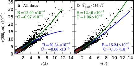
Figure 6: Fit of ${\tau(250\mu{\rm m})=A+B\times\tau(J)+C\times\tau(J)^{2}}$ to the combined data of all fields in which individual linear fits showed a strong correlation with $\delta k/k<0.2$. The blue and the green lines correspond to fits to the full column density range and to data points $\tau(J)>1.0$ alone, respectively. In the second frame, only data with colour temperatures below 14 K are used.

Figure 7 shows the error distributions of the parameters A–C. The fit was made to data $\tau(J)>1.0$ for all fields with a linear fit accuracy $\delta k/k<0.2$. In most fields, the formal error estimates of $\delta\tau(J)$ and $\delta\tau(250\mu{\rm m})$ are smaller than the actual scatter of points. Therefore we used the residuals of the linear fits before the MCMC calculation to determine a scaling factor, typically 2.0–3.0, that makes the error estimates in each field consistent with the actual scatter. Even after this increase of uncertainties, MCMC gives a 100% probability for a positive value of C. In reality, the result is not that strong because the uncertainty may be dominated by systematic errors. The sign of $C$ was already seen to change depending on the range of $\tau(J)$ values fitted. The result also depends on a relatively small number of fields with data above $\tau(J)>5$. Therefore, we must consider the $\tau(250\mu{\rm m})$ vs. ${\tau(J)}$ relation in individual fields in more detail.

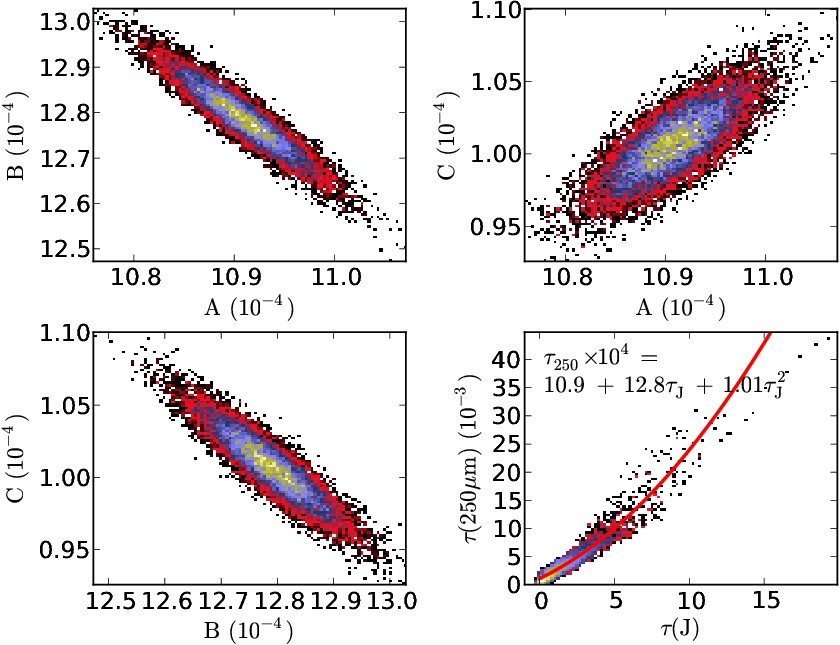
Figure 7: Distributions of the parameters of the fit $\tau(250\mu{\rm m})=A+B\times\tau(J)+C\times\tau(J)^{2}$. The fit is limited to data with $\tau(J)>1$.

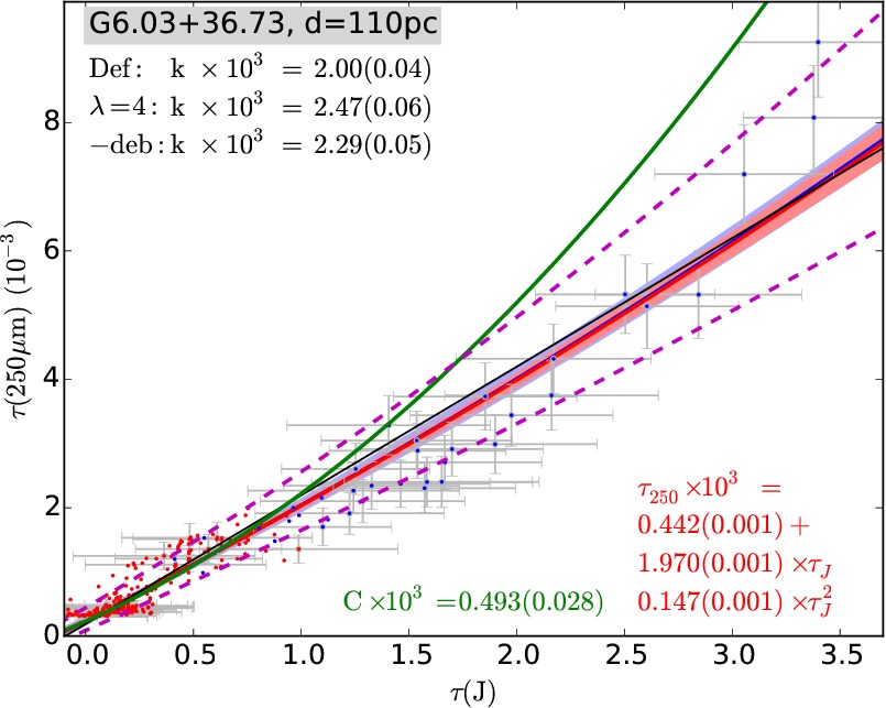
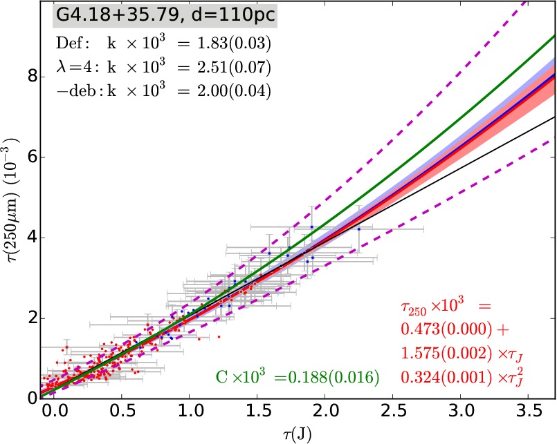
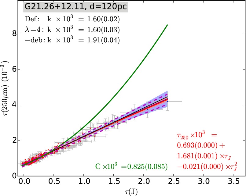
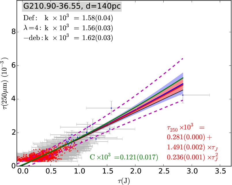
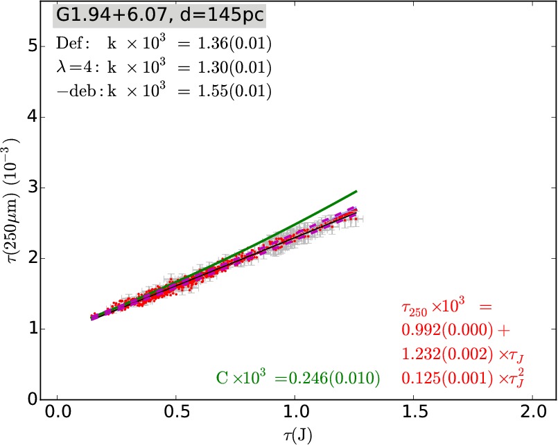
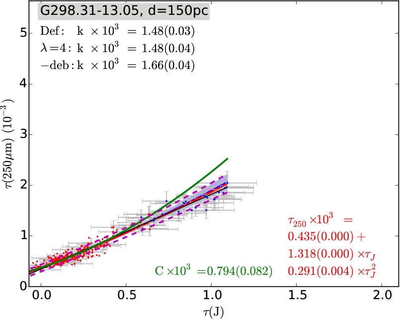
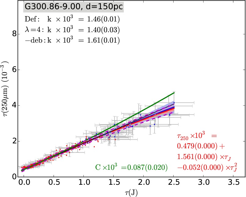
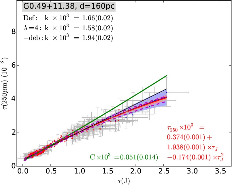
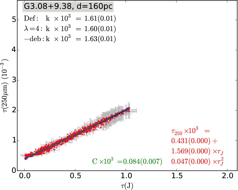
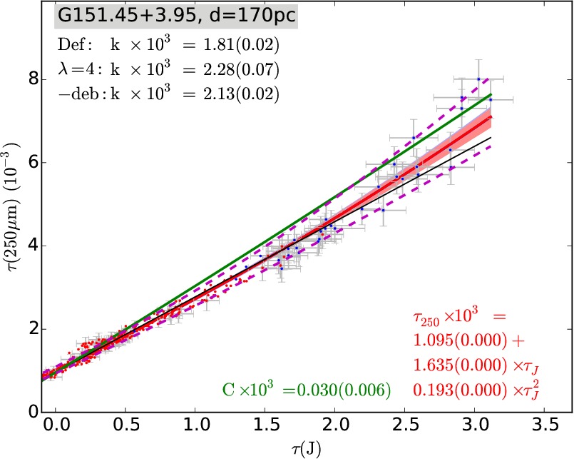
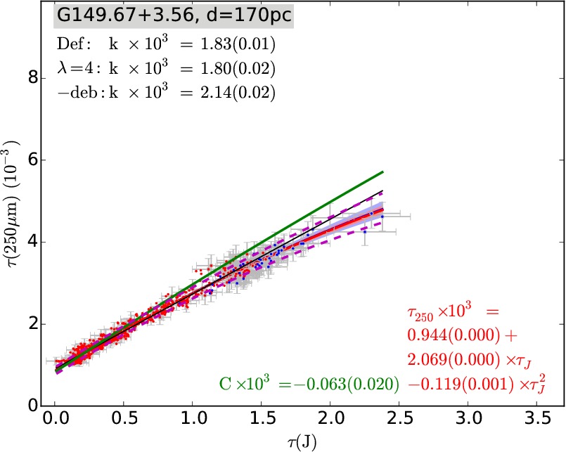
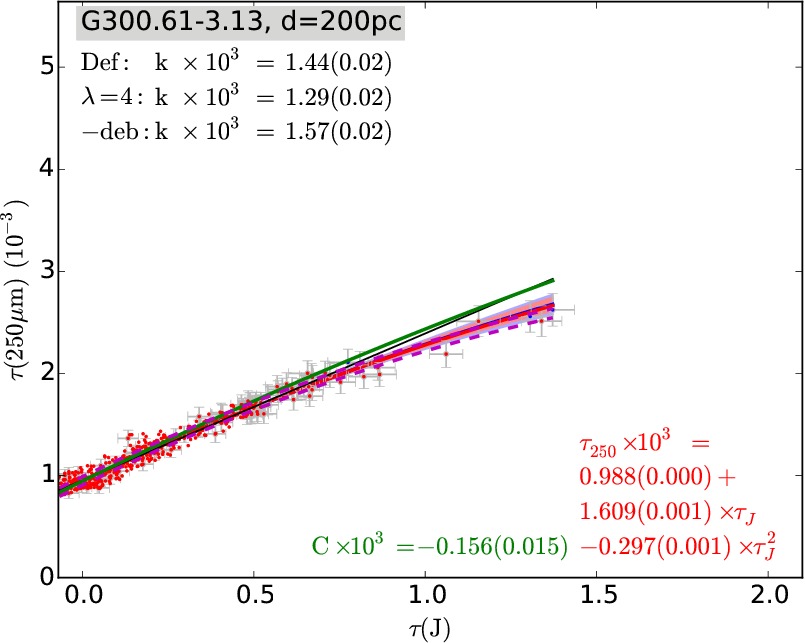
Figure 8: Fits of $\tau(250\mu{\rm m})$ vs. $\tau(J)$ in selected fields ordered by increasing distance. The red and blue points (dust temperature above and below 14 K) with error bars are the bias-corrected data points, where $\tau(250\mu{\rm m})$ is based on SPIRE data. The slopes of linear fits are listed in the upper left corner for (1) the default data set based on SPIRE data alone (“Def.”), (2) 160–500 $\mu$m data (“$\lambda$=4”), (3) SPIRE data but without bias corrections (“-deb”). The linear fit of the default case is shown with a black line. The non-linear fits are shown with solid blue lines (MCMC) and solid red lines (bootstrapping) with associated shaded 68 % confidence regions. The dashed magenta lines correspond to different bias correction of $\tau(J)$ using distances $d-\delta d$ and $d+\delta d$. The parameters from bootstrapping are given in the lower right corner. The non-linear fit to data without bias corrections is plotted with a solid green curve (without error region) with the parameter $C$ given at the bottom of the figure. The zero points of the ${\tau(J)}$ axes are not absolute.

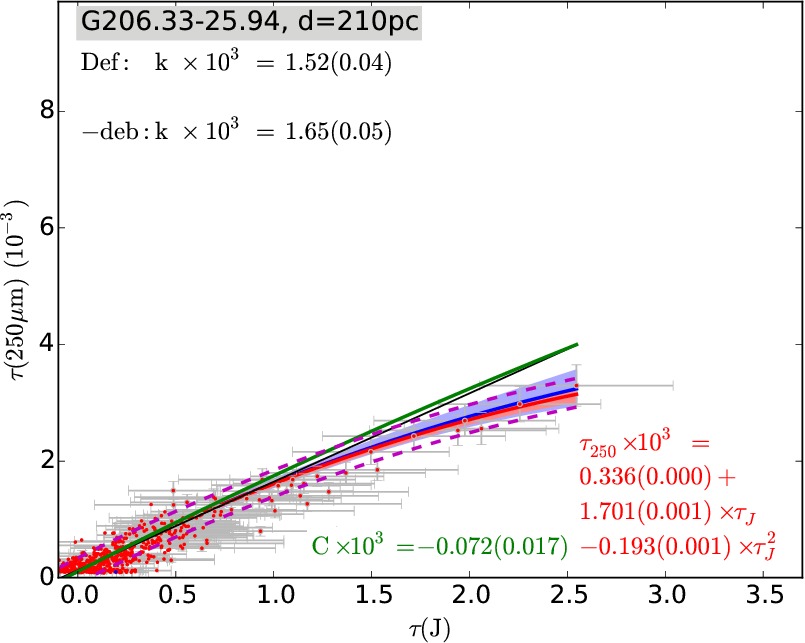
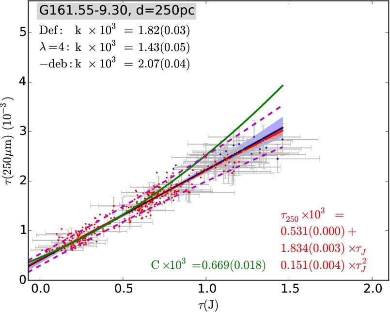
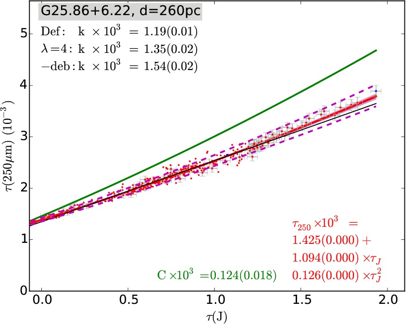
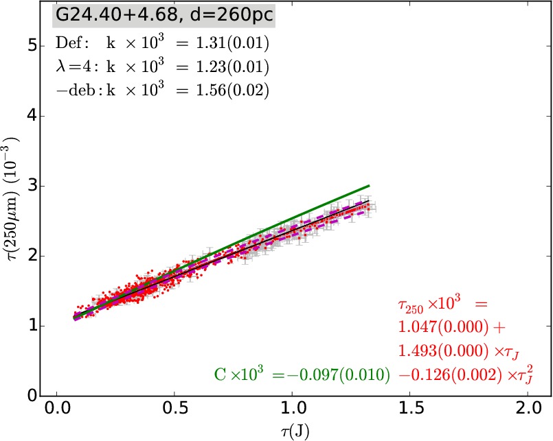
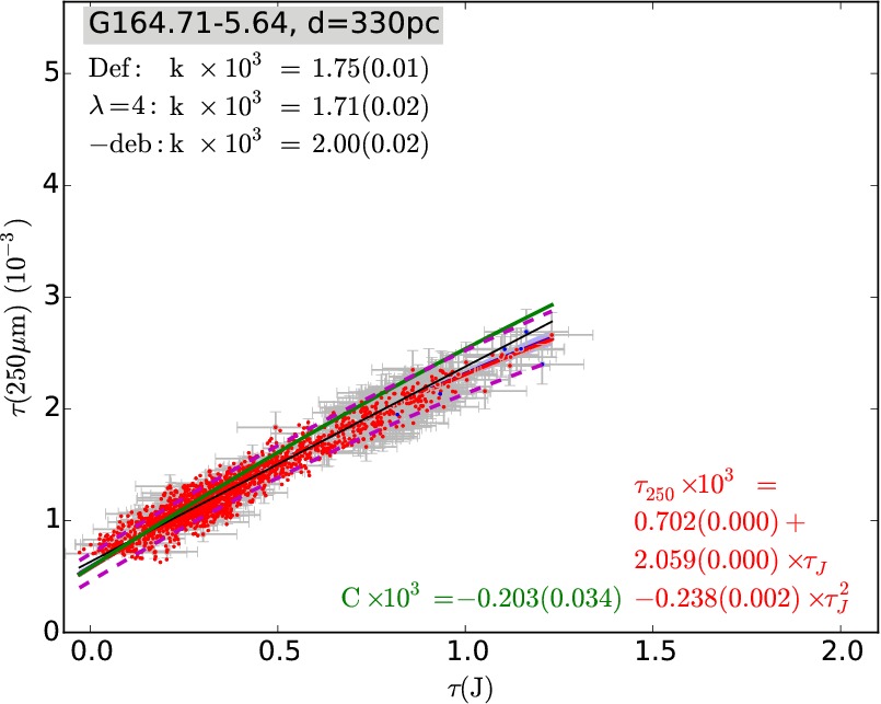
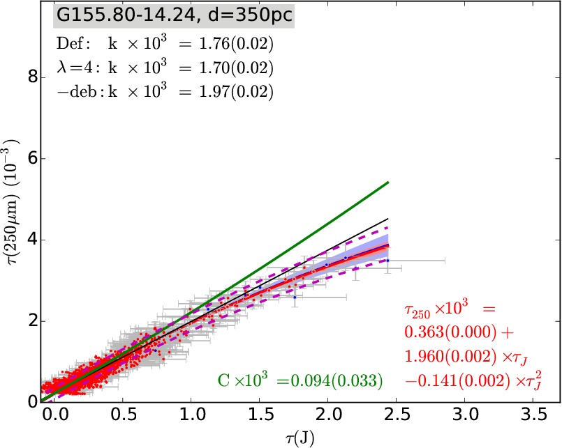
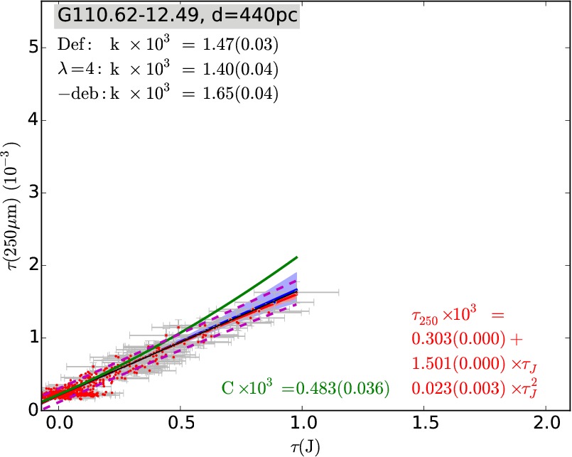
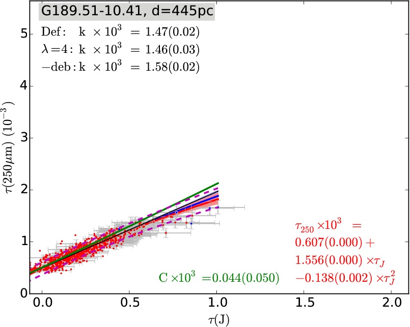
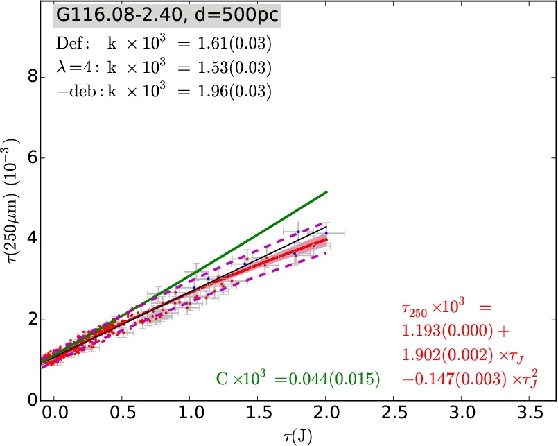
Figure 9: Continued…

3.5 Correlations in selected fields

Figure 6 showed hints of an increase of the ${\tau(250\mu{\rm m})/\tau(J)}$ values as the column density increases, but the global statistics may be confused by the mix of different fields. Furthermore, the sign of the $C$ parameter is determined by the highest ${\tau(J)}$ points that originate in a small number of individual fields. Each field may be affected by different systematic effects related to the surface brightness zero points, distance uncertainty (via bias correction), and differences in the local radiation field. Several diffuse fields are even entirely below $\tau(J)\sim 1.0$. Therefore, we also need to examine the fields individually.

Three criteria were used to select a subset of fields. We required that (1) the uncertainty of the fitted parameter $C$ is below ${\rm 0.3\times 10^{-4}}$, (2) there are at least ten data points (selected from the maps at 90$\arcsec$ steps) with $\tau(J)$ above 0.6, and (3) the bias corrections change the slope of the linear fit of ${\rm\tau(250\mu m)}$ vs. $\tau(J)$ by less than 30%. The first two criteria ensure that there are enough data points at large $\tau(J)$ with a small scatter to gain some insight about the column density dependence of the $\Delta\tau(250\mu{\rm m})/\Delta\tau(J)$. The third criterion excludes distant fields for which the uncertainty of the bias correction of $\tau(J)$ renders the results uncertain, even for the apparently well-defined relation between ${\tau(J)}$ and ${\rm\tau(250\mu m)}$. The selection leaves 23 fields with distances mostly in the range 100-500 pc. There are two exceptions, G216.76-2.58 and G111.41-2.95, for which the estimated distances are 2.4 kpc and 3.0 kpc. We kept the two fields in the sample even though the results are known to be unreliable because of the large distance.

To avoid underestimating the fit errors, we scaled the error estimates of $\tau(J)$ and $\tau(250\mu{\rm m})$ up to correspond to the actual scatter of points (see Sect. 3.4). All observations, sampled at 90$\arcsec$ steps, are fitted with a linear model ${\tau(250\mu{\rm m})=b+k\times\tau(J)}$ using total least-squares. We continued to use as the default data set one with $\tau(250\mu{\rm m})$ derived from SPIRE bands alone, including bias corrections in $\tau(250\mu{\rm m})$ and $\tau(J)$. However, for comparison, we also examined results obtained with four Herschel bands (160–500 $\mu$m; including the bias corrections) and, finally, with three Herschel bands but without any bias corrections.

The non-linear fits were made using MCMC (with $2\times 10^{5}$ samples per field) and bootstrap sampling (2000 realisations per field). Both fits used total least-squares and the error estimates of the individual points. The parameter values and the uncertainties derived with these two methods should be similar, except for rare cases in which the result depends on a small number of influential points, which are always present in the MCMC calculation, but not in all bootstrap samples.

Figures 8-9 show the results of these fits. Each frame shows the values of the linear slopes for the three cases discussed above. The parameters of the non-linear fits are shown together with the error estimates calculated with the bootstrap method. In addition to the fit to the default data set (solid red curve), the dashed magenta lines show the effect of the distance uncertainty. Using the distance uncertainties $\delta d$ listed in Table LABEL:table:fields, we also calculated the bias corrections for $\tau(J)$ for distances $d-\delta d$ and $d+\delta d$. Thus, the upper dashed line corresponds to distance $d-\delta d$ and a smaller bias correction.

Figure 10 shows the linear slopes $k$ and the values of parameter $C$ for this sample of fields. The fits were performed to all data, without a $\tau(J)$ threshold. If the data below $\tau(J)=0.6$ were removed, the median slope $\tau(250\mu{\rm m})/\tau(J)=1.6\times 10^{-3}$ did not change appreciably (by less than 0.1$\times 10^{-3}$). The median value of $C$ increased to $2.0\times 10^{-4}$, which in that case is still lower than the scatter. The differences between the fields are larger than the estimated formal uncertainties (including the statistical errors of $\tau(J)$ given by NICER and $\tau(250\mu{\rm m})$ derived from the uncertainty of the surface brightness measurements). The error bars only reflect the statistical errors of the fits and do not include the uncertainty of the bias correction, for example. Figure 8 demonstrates that the uncertainty of the distances can be a significant source of error. In Fig. 10, the shaded areas show the difference between the values obtained with distances $d-\delta d$ and $d+\delta d$, as listed in Table LABEL:table:fields. These were estimated directly by repeating the analysis using these two distance values. A smaller distance corresponds to smaller bias correction in $\tau(J)$ and, thus, to a steeper slope $k$ and typically a higher value of $C$. In some cases, the value of $C$ obtained with the default distance $d$ is outside the shaded region, showing that the effect is not always this simple. The distance uncertainty is not yet enough to explain all the scatter in $k$ and especially in $C$. A change in the distance estimate results at first approximation in a nearly linear scaling of $\tau(J)$ values (see Fig. 8, comparison of the dashed magenta lines). In reality, the situation may be more complex. In particular, if a field contains cloud structures at different distances, this might result in large errors in both $k$ and $C$. Figure 10 also shows that in spite of the small formal errors of the least-squares fits, we cannot constrain the opacity values in the last two fields with distances exceeding 2 kpc.

Figure 10: Linear slope $k$ (upper frame) and the parameters $C$ (lower frame) for the 23 selected fields. The values obtained without bias corrections are shown with black symbols. The values obtained with corrected $\tau(J)$ and ${\rm\tau(250\mu m)}$ data are shown with red symbols, the shaded area corresponding to the uncertainty of the bias correction that is due to the uncertainty of the distance estimates. The dashed lines show the median values corresponding to the black and red symbols. The fields are arranged in order of increasing distance, and the ${\rm\tau(250\mu m)}$ values are based on SPIRE data alone.

In the sample of Fig. 10, the median value of $C$ is close to zero with a number of fields with negative values. The positive values of $C$ in Fig. 6 are due to a small number of fields, and the increase of $\tau(250\mu{\rm m})/\tau(J)$ values was only visible above $\tau(J)\sim 5$. There are only 20 fields with any data points above $\tau(J)=5$. Only six fields have ten or more data points above this limit: G6.03+36.73, G70.10-1.69, G82.65-2.00 G92.04+3.93 G107.20+5.52, and G202.02+2.85. Of these, only G6.03+36.73 is included in the sample of Fig. 10. All the others were excluded because the bias correction changed the slope $k$ by more than 30%. Thus, a clear steepening of the relation $\tau(250\mu{\rm m}$ vs. $\tau(J)$ is seen exclusively in fields with the highest column densities, which for the same reason also have the largest uncertainty regarding the bias corrections.

3.6 Maps of $\tau(250\mu{\rm m})/\tau(J)$ ratio

We also examined the ratios $\tau(250\mu{\rm m})/\tau(J)$ in the form of maps. This is useful if $k$ changes in small regions that have little effect when all data of a field are fitted. Unlike in Fig. 8, where the offset between $\tau(250\mu{\rm m})$ and $\tau(J)$ is a free parameter, the appearance of the ratio maps depends on the consistency of the $\tau(250\mu{\rm m})$ and $\tau(J)$ zero points. Because we do not have an absolute zero point for $\tau(J)$, we used the reference areas listed in Table LABEL:table:fields and subtracted from $\tau(250\mu{\rm m})$ and $\tau(J)$ the average value found in the reference area. This limits the region where a reliable ratio can be calculated, excluding regions of low column density. The details of the calculations are given in Appendix E, where we also show the figures of selected fields. As an example, Fig. 11 shows the field G4.18+35.79 (LDN 134), where the ratio $\tau(250\mu{\rm m})/\tau(J)$ is strongly correlated with column density. In Fig. 11, the increase of $k$ remains clear even in maps of $(\tau(250\mu{\rm m})\pm\delta\tau(250\mu{\rm m})/(\tau(J)\pm\delta\tau(J))$. The error estimates $\delta\tau(250\mu{\rm m})$ include the statistical errors due to Herschel photometry and uncertainty of the surface brightness zero point (see Sects. 2.2.3 and 2.2.2). The parameter $\delta\tau(J)$ corresponds to the uncertainty of the $\tau(J)$ zero point (see Appendix E). For $\tau({\rm J})$ the formal error estimates calculated with NICER are below 10%.

For high-opacity sources like G4.18+35.79 the bias correction of $\tau(J)$ is very important. If no background stars are visible through some part of the core, the values of $k$ naturally remain more uncertain (see, however, Sect. 3.7). Conversely, the zero-point uncertainty only becomes important in diffuse regions but might even reverse the correlation with column density. The ratio maps are also affected by the assumption of a constant value of $\beta$ and of potential errors in the bias corrections. However, we argue in Sect. 3.7 that these are mainly multiplicative errors (that do not affect the morphology of the maps) and/or tend to decrease the variations seen in the ratio maps. Therefore, we are confident that the increase of submillimetre opacity that is seen in some of the maps is real.

Based on the maps, the submillimetre opacity is correlated with column density in the fields G4.18+35.79, G6.03+36.73, G111.41-2.95, G161.55-9.30, G151.45+3.95, and G300.86-9.00 (see Appendix E). In G4.18+35.79 and G6.03+36.73 the values rise to close to $4\times 10^{-3}$. In some fields the background subtraction reduces the available map area to such an extent that no conclusions can be drawn.

Figure 11: Field G4.18+35.79 (LDN 134). The upper frames show $\tau(250\mu{\rm m})$ (frame a) and the ratio $\tau(250\mu{\rm m})/\tau(J)$ (frame b). The lower frames show the lower (frame c) and upper (frame d) limits of $\tau(250\mu{\rm m})/\tau(J)$ calculated as $(\tau(250\mu{\rm m})+\delta\tau(250\mu{\rm m}))/(\tau(J)-\delta\tau(J))$ and $(\tau(250\mu{\rm m})-\delta\tau(250\mu{\rm m}))/(\tau(J)+\delta\tau(J))$. The areas not covered by Herschel observations and regions with a SN below 0.5 have been masked. In frame $a$, the solid black contour and the dashed white contour correspond to $\tau(250\mu{\rm m}=\delta\tau(250\mu{\rm m})$ and $\tau(J)=\delta\tau(J)$. The maps have a resolution of 180 $\arcsec$ and $\tau(J)$ is derived using 2MASS data.

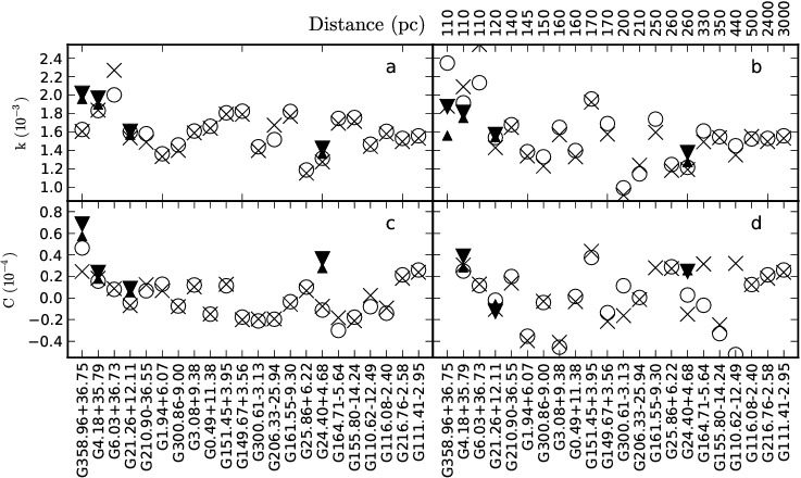
Figure 12: Comparison of parameters $k$ (upper frames) and $C$ (lower frames) obtained with data at resolutions of 180$\arcsec$ and 120$\arcsec$ . Frames $a$ and $c$ show fits to all data, frames $b$ and $d$ fits to values ${\tau(J)}>0.6$ alone. The open circles and crosses show the estimates obtained with 2MASS data at resolutions of 180$\arcsec$ and 120$\arcsec$ . The filled triangles show the results for VISTA observations, the larger triangles corresponding to a resolution of 180$\arcsec$ , the smaller to a resolution of 120$\arcsec$ . The fields are the same as in Fig. 10, with the addition of G358.96+36.75, which has fewer data points above ${\tau_{J}>0.6}$ and for which parameter $C$ could not be fitted with extinction maps with a resolution of 120$\arcsec$ .

So far, all NIR extinction maps were calculated at 180$\arcsec$ resolution. Depending on the number of background stars, extinction map could be derived at a higher resolution and possibly with smaller bias. This especially applies to the four fields for which VISTA observations are available. We recalculated the extinction maps at 120$\arcsec$ resolution, repeating Monte Carlo simulations to estimate the bias of ${\tau(J)}$. The smaller beam increases the noise per resolution element, but does not yet cause holes in the extinction maps. The analysis was repeated for the four fields with VISTA data with resolutions of 180$\arcsec$ and 120$\arcsec$ . The results are summarised in Fig. 12. The resolution has no strong systematic effect on the parameters. The largest differences appear when parameter $C$ is estimated excluding low column density points. However, even in that case the difference between the results with a resolution of 120$\arcsec$ and 180$\arcsec$ is smaller than the effect of excluding low $\tau(J)$ data from the fits. When VISTA data are available, the results are close to those obtained with 2MASS. Because we used the same Herschel data and bias corrections derived in the same way, the results are not independent. However, because the uncertainty of $\tau(J)$ is expected to be one of the most significant sources of error, this gives us some confidence that the observed differences between the fields are real.

The ${\tau(250\mu{\rm m})/\tau(J)}$ ratio in the field G4.18+35.79 was shown in Fig. 11. Figure 13 shows the corresponding figure obtained with VISTA NIR data and a spatial resolution of 120$\arcsec$. The highest value of ${\tau(250\mu{\rm m})/\tau(J)}$ has increased from $3.6\times 10^{-3}$ in Fig. 11 to $6.7\times 10^{-3}$. This is mainly attributed to the increased spatial resolution, although also at the 180$\arcsec$ resolution the peak value is $\sim$25% higher than in Fig. 11. Even in VISTA data there are only $\sim$10 stars within the $2\arcmin\times 2\arcmin$ area centred on the $\tau(250\mu{\rm m}$ maximum, and therefore the peak value of ${\tau(250\mu{\rm m})/\tau(J)}$ is subject to some uncertainty.

Figure 13: Ratio ${\tau(250\mu{\rm m})/\tau(J)}$ in field G4.18+35.79 at a resolution of 120$\arcsec$, based on VISTA NIR data. Frame $a$ shows a map of $\tau(250\mu{\rm m}),$ frame $b$ a map of the ratio $\tau(250\mu{\rm m})/\tau(J)$. Frames $c$ and $d$ are estimated lower and upper limits of $\tau(250\mu{\rm m})/\tau(J)$ (cf Fig. 11).

3.7 Potential systematic errors

Because of the significance of the bias corrections (Sects. 3.2 and 3.3), we tried to characterise the effects that systematic errors in these corrections could have on the $\tau(250\mu{\rm m})/\tau(J)$ ratios. Furthermore, the assumption of a constant dust emissivity spectral index may be incorrect. Below we examine the possible systematic effects caused by these factors.

The bias correction made to the ${\rm\tau(250\mu m)}$ values is in itself small (see Fig. 4) and, consequently, the errors made in that correction are expected to be small. The correction was derived from radiative transfer models with dust properties corresponding to $R_{\rm V}$=5.5 (Draine 2003b). If the submillimetre dust emissivity is in fact higher, the dust column density will be overestimated and models will also overestimate the cloud opacity at visual and NIR wavelengths, thus exhibiting stronger temperature variations than the real clouds. Because the ${\rm\tau(250\mu m)}$ bias is related to the line-of-sight temperature variations, we could in this case systematically overestimate the bias in ${\rm\tau(250\mu m)}$. To check the magnitude of the effect, we repeated the modelling using a dust model with higher long-wavelength emissivity. We used a dust model from Ossenkopf & Henning (1994) with coagulated grains with thin ice mantles accreted in 10⁵ years at a density of 10⁶ cm^-3. Compared to NIR (the wavelengths contributing to most of the heating deep inside a cloud), this dust model has an emissivity higher by $\sim$50% at SPIRE wavelengths. The results are shown in Fig. 14, the open circles corresponding to this alternative modelling. Because of the smaller estimated bias, these should be below the $k$ values of our previous analysis (red symbols). The median value of $k$ is 1.58$\times 10^{-3}$ and thus practically unchanged. The strongest change is seen for G6.03+36.73 (LDN 183), where the estimate has been reduced by more than 20%. This is a source with very high column density and thus, in its central parts, a very uncertain estimate of ${\rm\tau(250\mu m)}$. However, the uncertainty of ${\rm\tau(250\mu m)}$ bias must also be considered in connection with the uncertainty of the ${\tau(J)}$ correction, which could compensate for some of the change (see below).

The ${\tau(J)}$ bias corrections are more significant than the ${\rm\tau(250\mu m)}$ bias corrections. The estimation of the ${\tau(J)}$ bias is, in principle, more reliable because it only depends on the assumption of the ${\tau(J)}$ structure of the clouds. In our calculations (see Sect. 3.2), $\tau(J)$ was derived from Herschel observations, dividing ${\rm\tau(250\mu m)}$ by the constant factor of $k=$1.5$\times 10^{-3}$ to obtain a template map of $\tau(J)$. There are two possible sources of error. First, if the targets contain much structure below the 18$\arcsec$ resolution of the ${\rm\tau(250\mu m)}$ maps, we will underestimate the bias and our $k$ estimates will be too high. We cannot directly estimate this error, but it is expected to be a small fraction of the total bias estimate. This is because $18\arcsec\ll 3\arcmin$ and, at least for the closest fields, Herschel already resolves most of the cloud structure. The second potential source of error is again connected with dust emissivity. If the local ratio between ${\rm\tau(250\mu m)}$ and ${\tau(J)}$ is higher than 1.5$\times 10^{-3}$ (strongly increased submillimetre opacity), we have overestimated the cloud opacity at NIR wavelengths in the modelling, the bias correction of ${\tau(J)}$ is too large, and we underestimate the true value of $k$. Thus, a change in the value of $k$ that is used to estimate the ${\tau(J)}$ bias will change the recovered value of $k$ in the same direction. To examine this potential problem more quantitatively, we repeated the bias estimation using $k$ values of 1.0$\times 10^{-3}$ and 3.0$\times 10^{-3}$. The resulting values of $k$ and $C$ parameters are shown in Fig. 14 as triangles. The initial assumption of $k=$1.0$\times 10^{-3}$ leads to a recovered median value of $k=$1.26$\times 10^{-3}$. The initial assumption of $k=$3.0$\times 10^{-3}$ leads to a recovered median value of $k=$1.92$\times 10^{-3}$. In both cases the input and output values are inconsistent, unlike in our previous analysis, where an assumption of 1.5$\times 10^{-3}$ led to a recovered value of 1.6$\times 10^{-3}$. Furthermore, an error in the assumed value of $k$ leads to a systematic error in the recovered value that is about half of the original error, even lower if the true value of $k$ was initially overestimated.

The previous test shows that the estimates of $k$ will be biased towards the selected value of 1.5$\times 10^{-3}$. Our previously recovered median value of 1.6$\times 10^{-3}$ is thus not significantly affected (bias lower than 0.05), but the effect can be stronger for individual fields. For example, in G4.18+35.79 the estimate was 1.8$\times 10^{-3}$ , but the true value is probably higher by $\sim$10%. The calculations could be iterated, field by field, to carry out the bias correction self-consistently with the final $k$ estimate. However, the errors are typically below 10%, and rough estimates of their magnitude can be seen in Fig. 14.

There is a specific consequence of the way the $\tau(250\mu{\rm m})$ and ${\tau(J)}$ bias corrections are implemented. If a cloud included regions of such a high opacity that no 2MASS stars were visible through the cloud, the ratio of $\tau(250\mu{\rm m}$ and $\tau(J)$ would normally be overestimated. The resulting apparent increase of submillimetre opacity could thus be an artefact resulting from errors in extinction values. However, in our analysis we also correct ${\tau(J)}$ in this case based on the assumed opacity derived using the $\tau(250\mu{\rm m})$ input map and the extinction calculated with simulated 2MASS stars. If the gap in the distribution of background stars is increased, the ratio $\tau(250\mu{\rm m})/\tau(J)$ does not continue to increase, but instead tends towards the assumed ratio, 1.5$\times 10^{-3}$. Higher values should thus not be the result of gaps in extinction data.

To investigate the potential effects of a spatially varying spectral index, we repeated the analysis using an ad hoc $\beta(T)$ law to introduce $\beta$ variations in all of our maps. We took the temperatures calculated with $\beta=2.0$ and fixed new $\beta$ values pixel by pixel using a functional dependence $\beta=2.0\times(T/15.0)^{-0.24}$. We then repeated the full analysis, starting with the zero point and colour corrections and continuing with the calculation of colour temperatures and submillimetre opacity. We did not solve the ($T$, $\beta$) values (which are very susceptible to noise effects), but simply assumed that $\beta$ could vary in a systematic way so that the values are higher when the dust temperature is lower. The parameters of the $\beta(T)$ formula were selected so that $\beta$ changes from $\sim 1.8$ in warm regions with $T\sim 23$ K to $\sim 2.2$ in the coldest spots $T\sim 10$ K (cf Dupac et al. 2003; Désert et al. 2008; Planck Collaboration XXIII 2011; Paradis et al. 2010; Veneziani et al. 2010; Juvela et al. 2011). The average $\beta$ is still close to the original $\beta=2.0,$ and we mainly examined the effects of correlated changes of $\beta$ rather than the effects of absolute $\beta$ values that can be estimated more directly. The crosses in Fig. 14 show the slopes $k=\Delta\tau(250\mu{\rm m}/\Delta\tau(J)$ and the parameters $C$ obtained with the spatially varying $\beta$. The values are typically within $\sim$10% of the values obtained with $\beta=2.0$. The strongest changes of $k$ are seen in the two closest fields, G4.18+35.79 and G6.03+3673, which have well-resolved clumps with very low temperatures. The increase of the slope values is $\sim$20%. Note that this is mostly consistent with the general dependence between $\tau(250\mu{\rm m})$ and $\beta$ and not necessarily an effect of the spatial variation of $\beta$. In this respect, it is very interesting to note that the effect on the parameter $C$ is weak. In other words, if the variations of $\beta$ are as assumed above, this will be reflected in the slope $\tau(250\mu{\rm m})/\tau(J),$ but without a noticeable non-linearity in the $\tau(250\mu{\rm m})$ vs. $\tau(J)$ relation.

All the above suggests an uncertainty of 10–20% in $k$ and $\sim$0.1 units in $C$. In particular, if the increase of dust opacity is associated with values $\beta>2.0$, our highest $k$ estimates could still systematically underestimate the true values of $k$ because of the lower assumed value of $\beta$ and because the $\tau(J)$ correction biases the $k$ values towards 1.5$\times 10^{-3}$.

Figure 14: As Fig. 10, but comparing our default $\tau(250\mu{\rm m})/\tau(J)$ estimates (red solid circles) and results from alternative analyses: $\tau(250\mu{\rm m}$ estimates derived assuming a spatially varying spectral index (crosses), $\tau(250\mu{\rm m}$ bias estimated with Ossenkopf & Henning (1994) dust model (open circles), $\tau(J)$ bias estimated using $k=1.0\times 10^{-3}$ (triangles pointing upwards), and $\tau(J)$ bias estimated using $k=3.0\times 10^{-3}$ (triangles pointing downwards).

4 Discussion

We have examined the submillimetre opacity by correlating the 250 $\mu$m optical depth ${\rm\tau(250\mu m)}$ with the near-infrared optical depth, $\tau(J)$, assuming the latter to be an independent tracer of the total dust column density. Because the comparison was made at a resolution of 2$\arcmin$ , it is not sensitive to dense cores ($A_{\rm V}>>10$ mag), at which both the ${\rm\tau(250\mu m)}$ and $\tau(J)$ estimates would become very uncertain. Nevertheless, corrections for systematic bias in ${\rm\tau(250\mu m)}$ and especially in $\tau(J)$ are important.

The sample consists of the heterogeneous set of 116 Galactic fields that were mapped with Herschel as part of the Galactic Cold Cores project. The main objectives were to estimate the typical ratio of ${\rm\tau(250\mu m)/\tau(J)}$ and to search for variations of this quantity, between the fields and as function of column density. Such variations were then related to differences in the properties of interstellar dust grains. For the present sample, high column densities also imply low dust temperatures and thus conditions where submillimetre dust opacity is expected to be enhanced by grain aggregation. The limited resolution means that we did not probe the full range of opacity variations, if these are partly limited inside compact cores.

4.1 Main results and their reliability

By restricting the analysis to $\sim$20 fields for which the results appeared most reliable, we derived a median value of $k={\rm\tau(250\mu m)/\tau(J)=1.6\times 10^{-3}}$ (see Sect. 3.5 and Fig. 10). In Fig. 10, 50% of the most nearby fields had positive values of $C$, the multiplier of the second-order term, indicating some degree of positive correlation between column density and submillimetre emissivity measured by $\tau(250\mu{\rm m})$. In the maps of the ratio $k$, the same tendency was very clear in only six cases. The low percentage is partly caused by the noise in ${\tau(J)}$, whose magnitude is strongly correlated with the cloud distances. For two of the best examples, G4.18+35.79 and G6.03+36.73, the ratio ${\rm\tau(250\mu m)/\tau(J)}$ increases to $\sim 4\times 10^{-3}$, almost a factor of three higher than the median value. The peak values are uncertain because of the large bias corrections, but because of the low spatial resolution used, the strongest effect can be even greater.

No dependence on either Galactocentric distance or on Galactic height was observed (Fig. 5). The reliability of the estimates decreases with distance, but nevertheless, our sample extends over more than $\sim$4 kpc in Galactocentric distance. No trends are seen; if they were present at 10% level, they should still be visible over the scatter of individual data points. The result might be affected by systematic errors in the bias correction. However, these probably depend either on the distance or on the morphology of the field and at first approximation are not expected to be different in the inner and in the outer Galaxy.

In Fig. 10, the only clear trend is the decrease of $k$ as a function of distance (also visible as larger scatter around the Galactocentric distance of 8.5 kpc). As mentioned in Sects. 3.2 and 3.3, there are two possible explanations. First, the bias correction of $\tau(J)$ might be overestimated so that as the distance increases, the error increases and $k$ becomes underestimated. This is probably not the main reason because the bias correction depends as much on column density values and column density gradients as on distance. The trend probably is a combination of selection and resolution effects. At 1 kpc the 180$\arcsec$ resolution corresponds to almost 1 pc in linear scale. Therefore, we measure the mean cloud properties for the most distant fields. In the nearby fields individual clumps are resolved and the slopes $k$ reflect more the contrast between diffuse regions and compact, core-sized objects. Thus, the trend would be compatible with the hypothesis that $\tau(250\mu{\rm m})/\tau(J)$ increases in the densest and coldest regions of interstellar clouds.

The global non-linear fits of Fig. 6 also indicated an increase of the ratio $k=\tau(250\mu{\rm m})/\tau(J)$ as the function of column density. The plots show clear deviations from a linear dependence beyond $\tau(J)\sim 4$. For $\tau(J)\sim 10$, $k$ is already twice as high at low column densities. The results are dependent on a few fields with the highest column densities for which the bias corrections reach about ten per cent. However, if the distance dependence of Fig. 5 means that the bias correction of ${\tau(J)}$ is probably overestimated and not underestimated, the true values of $k$ might be even higher.

Figure 10 concentrated on selected fields for which linear and non-linear fits were more reliable than on average. Within this subset, no clear distance dependence was visible in $k$ values, but the scatter is larger than the estimated uncertainties. The linear slopes are sensitive to the highest column densities within a field. The parameter $C$ of the non-linear fits is expected to be even more sensitive to these data points, which probe the variations of $\tau(250\mu m)/\tau(J)$ inside the fields. For the whole sample, the median value of $C$ was very close to zero. Nevertheless, it may be significant that when the two fields at kiloparsec distances are excluded, the value of $C$ appears to decrease somewhat systematically with the distance of the field. There is some preference for the most nearby fields to have positive values; here, the densest parts of the clouds are resolved.

Two of the first fields with high $k$ values are G6.03+36.73 and G4.18+35.79, better known as LDN 183 and LDN 134. At the Herschel scale, the clouds have a simple morphology, each consisting of a single column density maximum that is partially resolved by the 180$\arcsec$ beam. This is illustrated by Figs. 11 and 18. The ratio $k=\tau(250\mu{\rm m})/\tau(J)$ closely follows the morphology of the column density distribution, making these the best examples of clumps with increased submillimetre opacity. The highest values are $\sim 4\times 10^{-3}$, almost three times the average value over all fields.

In our results, some of the main sources of uncertainty are the corrections made for the expected bias in $\tau(J)$ and, to lesser extent, in ${\rm\tau(250\mu m)}$. According to Fig. 10, the net effect of all bias corrections is a $\sim$20% decrease in the value of $k$. This number applies to nearby fields but is more dramatic if all fields are taken into account. Figure 5 shows that for fields at $\sim$1 kpc distance the correction is almost a factor of two. The corrections have been remarkably successful in decreasing the scatter of $\tau(250\mu m)/\tau(J)$ values, which strongly suggests that they are approximately of the correct magnitude.

In the statistical sense, estimating the ${\tau(J)}$ bias is straightforward, using a model of the Galactic stellar distribution and the higher resolution Herschel data as a template for the column density structure of the field (see Appendix B and Sect. 3.7). The correction is large, but on average, the correction itself probably does not suffer from major systematic errors. Errors could arise either from incorrect distance estimates or from the use of an incorrect model of the NIR opacity distribution. The distances are uncertain, and through the ${\rm\tau(J)}$ bias, their effect on the main parameters is shown in Fig. 10 (the grey bands) and in Fig. 8. For a sample of fields, this is mainly a statistical and not a systematic error.

The model of $\tau(J)$ distribution in each field was derived from Herschel data at 18$\arcsec$ resolution. If there is still significant structure below this scale, our correction of $\tau(J)$ values will be too low. The difference of the 2-3$\arcmin$ scale and the 18$\arcsec$ scale is so large, however, that most of the effects of column density variations are already included. Thus, after the distance, the other main error in the $\tau(J)$ bias correction arises from scaling the Herschel estimates of ${\rm\tau(250\mu m)}$ into a template of the J-band opacity. We showed in Sect. 3.7 that this amounts to an uncertainty of $\sim$10% in the final listed values of $k=\Delta\tau(250\mu{\rm m})/\Delta\tau(J)$. For the sample in Fig. 10, the value of $k$ assumed during the bias correction is consistent with the recovered value (to be precise, the assumed value of $k=1.5\times 10^{-3}$ , the recovered value of $k=1.6\times 10^{-3}$). For individual fields, the values are biased towards the initial assumed value. Figure 14 showed that if bias correction assumed a value of $k=1.0\times 10^{-3}$, the recovered median value was still higher than $k=1.2\times 10^{-3}$. This shows that $k$ cannot be significantly overestimated because of an erroneous bias correction in $\tau(J)$. Thus, the result that the average ratio $k=\Delta\tau(250\mu m)/\Delta\tau(J)$ is clearly higher than the normal value found in diffuse medium remains robust.

Because of the bias in the $\tau(J)$ correction, our estimates are probably conservative for fields where values $k>1.5\times 10^{-3}$ were obtained. The dependence on the assumed value of $k$ decreases as the true value of $k$ increases. This is because higher $k$ means a lower NIR opacity and lower overall bias in $\tau(J)$. Nevertheless, for fields like G4.18+35.79, we might systematically underestimate $k$ by $\sim$10% because of this error in the $\tau(J)$ bias correction. At the highest column densities Herschel emission data themselves will underestimate the cloud opacity, which leads to the corrections discussed in Sect. 3.3. For the optical depth ratio, the effect of ${\rm\tau(250\mu m)}$ bias is weaker than that of $\tau(J)$. Nevertheless, the errors made in the corrections of ${\rm\tau(250\mu m)}$ and $\tau(J)$ (for example, those associated with a change of submillimetre opacity) would partly cancel each other out.

In the analysis we assumed that apart from the problems associated with the sampling provided by the background stars, NIR reddening is an independent and reliable measure of column density. Unlike in the optical range, the NIR extinction curve is often assumed to be constant for a wide range of column densities (Cardelli et al. 1989; Martin & Whittet 1990; Roy et al. 2013). Nevertheless, some cloud-to-cloud variations are observed, the ratio $E_{J-H}/E_{H-K}$ ranging from values lower than 1.5 to higher than 2.0 (Racca et al. 2002; Draine 2003a). Clear changes take place at high optical depths, above $A_{\rm V}\sim 20$ mag, but only in the form of the flattening of the MIR extinction curve, at wavelengths above 3 $\mu$m (Indebetouw et al. 2005; Cambrésy et al. 2011; Ascenso et al. 2013). Recently, Whittet et al. (2013) studied cloud LDN 183 (which is also included in our sample). Comparison with the 9.7 $\mu$m silicate absorption feature suggested that the NIR colour excess might not be a perfect tracer of the total dust column. The ratio between $E_{J-K}$ and the 9.7 $\mu$m feature was observed to increase as the column density exceeded $A_{\rm V}\sim$20 mag. The observation might partly arise because the 9.7 $\mu$m feature is dampened by the formation of ice mantles (see also Chiar et al. 2007). However, if we assume that NIR extinction indeed overestimates the total dust column in this object, the ratio of ${\rm\tau(250\mu m)}$ relative to column density would increase by $\sim$20% (see Whittet et al. 2013, Fig. 12). This is still a weaker effect than the increase by more than a factor of two that was observed in $\tau(250\mu{\rm m})/\tau(J)$. We recall that at high column densities, above $A_{\rm V}\sim 20$ mag, the values of ${\rm\tau(250\mu m)}$ are also uncertain and can be underestimated by a significant fraction (Pagani et al. (2004) discussed a similar limitation at the nearby wavelength of 200 $\mu$m).

Finally, we recall that $\tau(250\mu{\rm m})$ values were derived using a fixed value of the spectral index, $\beta=2.0$. By assuming $\beta=1.8$ instead, the $\tau(250\mu{\rm m})$ and $k$ values would decrease by up to 30%. Conversely, if the value of $\beta$ increased towards dense and cold regions (Dupac et al. 2003; Désert et al. 2008; Planck Collaboration XXIII 2011; Paradis et al. 2010; Veneziani et al. 2010; Juvela et al. 2011), we underestimate the dust opacity changes if we use a constant value of $\beta$ . In this sense (and regarding possible bias in ${\tau(J)}$ corrections), Figs. 6–8 give conservative estimates of the possible increase of submillimetre dust opacity. Clearly, the assumed values of $\beta$ must also be taken into account when comparing our results with other studies (see Sect. 4.2). On the other hand, our tests indicate that spatial variations of $\beta$ probably do not have a strong additional effect on $k$ (see Sect. 3.7).

4.2 Comparison with other studies

The submillimetre dust opacity has previously been studied in relation to both dust extinction (Terebey et al. 2009; Flagey et al. 2009; Juvela et al. 2011; Martin et al. 2012; Roy et al. 2013; Malinen et al. 2013, 2014) and to HI (Boulanger et al. 1996; Lagache et al. 1999; Planck Collaboration XXIV 2011; Planck Collaboration XXV 2011; Martin et al. 2012). Boulanger et al. (1996) compared COBE observations of FIR dust emission with the hydrogen 21 cm observations. At high latitudes, where HI is a good tracer of the full gas column density, the derived value was $\tau/N_{H}=1.0\times 10^{-25}\,(\lambda/250\mu{\rm m})$ cm² H^-1. Similar values were obtained in the first studies using Planck data (Planck Collaboration XXIV 2011).

In the most recent Planck papers, somewhat lower values were reported, corresponding to $\tau(250\mu{\rm m})/N_{\rm H}\sim 0.55\times 10^{-25}$ cm² H^-1 (Planck Collaboration XI 2014; Planck Collaboration Int. XVII 2014). The change is associated with the revised calibration of the highest frequency channels and, correspondingly, a lower value of $\beta$. In Planck Collaboration Int. XVII (2014) the spectral index above 353 GHz was found to be $\beta\sim 1.65$, lower than the value of 1.8 assumed in Planck Collaboration XXIV (2011) or the value of 2.0 used in Boulanger et al. (1996). The higher dust opacity value of Boulanger et al. (1996) is thus largely explained by the higher value of $\beta$.

The Planck result for the diffuse medium can be compared to our result most directly by converting their $N_{\rm H}$ to $\tau(J)$. We can use the conversion factor $N({\rm H}_{2})/A_{\rm V}=9.4\times 10^{20}$ cm^-2 mag^-1 derived by Bohlin et al. (1978) at low extinction, $E(B-V)$¡0.5 (see also Nozawa & Fukugita 2013). Some studies (Rachford et al. 2009; Planck Collaboration XI 2014; Liszt 2014) have found $N_{\rm H}/E(B-V)$ values that are 10–30% higher than in Bohlin et al. (1978), these results apply partly to even more diffuse lines of sight ($E(B-V)\la 0.1$). On the other hand, Gudennavar et al. (2012) examined a sample of lines of sight with $E(B-V)$ extending to values higher than one. The result, $N({\rm H})/E(B-V)=(6.1\pm 0.2)\times 10^{21}$ H cm^-2 mag^-1, was close to that of Bohlin et al. (1978). With the Bohlin et al. (1978) relation and $R_{\rm V}=3.1$ extinction curve (Cardelli et al. 1989), the Planck result $\tau(250\mu{\rm m})/N_{\rm H}\sim 0.55\times 10^{-25}$ cm² H^-1 Planck Collaboration XI (2014) corresponds to ${\tau(250\mu{\rm m})/\tau(J)}=0.41\times 10^{-3}$. Our median value of ${\tau(250\mu{\rm m})/\tau(J)}=1.6\times 10^{-3}$ is thus 3.9 times higher, and our highest local values, 4.5$\times 10^{-3}$ in G4.18+35.79, are higher by one order of magnitude. In Planck Collaboration XI (2014) the estimated value of $N({\rm H}/E(B-V))$ was $\sim$20% higher than in Bohlin et al. (1978). With this value, our median value of ${\tau(250\mu{\rm m})/\tau(J)}$ would be $\sim 3.3$ times higher than the Planck estimate.

We can alternatively convert our result into $\tau(250\mu{\rm m})/N_{\rm H}$ , but in dense regions the shape of the extinction curve (dependence on $R_{\rm V}$) and the ratio between visual extinction and total column density are more uncertain. Using the $R_{\rm V}=3.1$ and $N({\rm H}_{2})/A_{\rm V}$ from Bohlin et al. (1978), our median value corresponds to $\tau(250\mu{\rm m})/N_{\rm H}=2.16\times 10^{-25}$ cm² H^-1 (again, of course, 3.9 times the Planck value). However, $R_{\rm V}$ is expected to be higher than 3.1 in dense clouds. Using $R_{\rm V}=5.5$ instead of $R_{\rm V}=3.1$ in converting $\tau(J)$ into visual extinction, the values of $\tau(250\mu{\rm m})/N_{\rm H}$ would decrease by $\sim 15$% (change in $A_{\rm V}/E(J-K)$). However, the scaling we used above (corresponding to the $R_{\rm V}$=3.1 extinction curve and the ratio of $N({\rm H}_{2})/A_{\rm V}$ taken from Bohlin et al. (1978)) corresponds to $N({\rm H})/E(J-K)=11.0\times 10^{21}$ cm^-2 mag^-1, which is very close to the value of $11.5\times 10^{21}$ cm^-2 mag^-1 that Martin et al. (2012) derived in Vela molecular cloud using 2MASS NIR data up to $E(J-K)\sim 0.55$ mag ($E(B-V)\sim 1.1$ mag).

When $R_{\rm V}$ is modified, the NIR extinction curve remains practically unchanged and the differences take place between the optical and NIR wavelengths. Compared to shorter (optical) and longer (MIR) wavelengths, the extinction curve is considered relatively constant in the NIR regime (e.g. Indebetouw et al. 2005; Lombardi et al. 2006; Román-Zúñiga et al. 2007; Ascenso et al. 2013; Wang & Jiang 2014) and the power-law slope of the NIR extinction curve typically only varies at a level of $\sim$5% (Stead & Hoare 2009; Fritz et al. 2011). In very dense cores the formation of ice mantles and the grain growth could have an additional impact. Román-Zúñiga et al. (2007) examined the cloud Barnard 59 up to $A_{\rm V}=59$ mag, but found no significant changes in the NIR extinction law (compatible with $R_{\rm V}=5.5$). Similarly, Lombardi et al. (2006) found no changes in the Pipe nebula in the reddening NIR law up to $E(H-K)\sim 1.5$ mag ($A_{\rm V}\sim 9$ mag). Therefore, it is not likely that our results are significantly biased because of the assumed NIR extinction curve. At the resolution of our extinction maps, practically all our data points are lower than$A_{\rm V}\sim 10$ mag and are thus not affected by extreme optical depths. However, Whittet et al. (2013) observed a decrease in L183 in the ratio of $E(J-K)$ and the 9.7 $\mu$m silicate absorption feature. Above $E(J-K)\sim 1.0$ ($A_{\rm J}\sim 1.7$ mag, $A_{\rm V}\sim 5.0$ mag for $R_{\rm V}=5.0$), the ratio deviated from diffuse medium value by $\sim 20$%. Stronger deviations were only seen beyond $E(J-K)\sim 3$ ($A_{\rm J}\sim 5$ mag, $A_{\rm V}\sim 15$ mag for $R_{\rm V}=5.0$). This is above the range probed by our measurements. It is not clear that changes in this ratio would only be caused by the NIR extinction curve. However, if, in some sources, the extinction curve does flatten above $A(J)\sim 2$, this might contribute to the observed increase of $\tau(250\mu{\rm m})/\tau(J)$ (possibly at the 20% level).

The effect of the bias corrections on $\tau(250\mu{\rm m})/\tau(J)$ is typically $\sim$20% or weaker, and their uncertainty is smaller. The largest uncertainties in $\tau(250\mu{\rm m})/N_{\rm H}$ are caused by $\beta$ and possibly by $R_{\rm V}$. With $\beta=1.8$ and $R_{\rm V}$=5.5, the $\tau(250\mu{\rm m})/\tau(J)$ values would be 40% lower than with $\beta=2.0$ and $R_{\rm V}$=3.1. At this lower limit, our median value of $\tau(250\mu{\rm m})/\tau(J)$ would not be 3.9 times, but $\sim$2.3 times the value found in the diffuse high-latitude sky. The 40% uncertainty may be a realistic 1 $\sigma$ lower limit for the linear fits that include all pixels in the maps. However, it is a conservative estimate for the clumps where the average value of $\beta$ is expected to be clearly higher than 1.8. In fact, preliminary results indicate that the average value of $\beta$ in our fields (including the more diffuse regions) is close to $\beta=1.9,$ and that with $\beta=2.0$ we underestimate the $\tau(250\mu{\rm m})$ values of many clumps (Juvela 2014 in preparation).

Increased far-infrared and submillimetre opacity has been reported by many authors (Kramer et al. 2003; Lehtinen et al. 2004; del Burgo & Laureijs 2005; Ridderstad & Juvela 2010; Bernard et al. 2010; Suutarinen et al. 2013, etc.). One famous example is the Taurus filament L1506, for which the models of Stepnik et al. (2003) suggested an increase by more than a factor of three. With the recent detailed modelling of the dust properties and the structure of this filament, Ysard et al. (2013) estimated the increase of the 250 $\mu$m opacity to be $\sim$2. Martin et al. (2012) studied the relation in the Vela cloud, comparing BLAST and IRAS data with the reddening of 2MASS stars. The properties of the examined areas corresponded to the average properties of our fields, with column densities extending to $10^{22}$ cm^-2 and with typical dust temperatures of $\sim 15\,K$. They found a very similar range of dust opacities, $\tau(250\mu m)/N_{\rm H}=(2-4)\times 10^{-25}$ cm² H^-1 (assuming $\beta=1.8$). In the Orion A cloud, a comparison of Herschel and 2MASS data led to the detection of a dependence of $N^{0.28}$ on the 250 $\mu$m opacity (Roy et al. 2013). The range of column densities in Orion A was similar to our fields, and the derived dust opacities were mainly in the range of $\tau(250\mu m)/N_{\rm H}=(1-3)\times 10^{-25}$ cm² H^-1. These estimates were derived with $\beta=1.8$ and would become $\sim 20$% higher (depending on the details of the fitting) if a value of $\beta=2.0$ were used. More recently, Lombardi et al. (2014) derived ratios $A({\rm K})/\tau(850\mu m)$ of 2640 mag and 3460 mag for the Orion A and B molecular clouds, respectively. The 850 $\mu$m optical depth was derived from Herschel observations rescaled using a comparison with Planck measurements, and the NIR extinction was calculated with the method NICEST (Lombardi 2009). The modified blackbody fits used $\beta$ values that were estimated in Planck Collaboration XI (2014) at a resolution of 30$\arcmin$. With the reported average value of $\beta=1.8$ and adopting a ratio 0.40 between $A({\rm K})$ and $A({\rm J})$, the results correspond to ${\rm\tau(250\mu m)/\tau(J)}$ values of $1.56\times 10^{-3}$ and $1.19\times 10^{-3}$ for Orion A and B, respectively. These fits were made for data ${\rm\tau(850\mu m)}<2\times 10^{-4}$ (${\rm\tau(250\mu m)}\la 1.8\times 10^{-3}$). The optical depth range is similar to many of our fields, and the result for Orion A is close to our median value for the fits concerning entire fields. By adopting $\beta=1.8$, our median value would fall between the Orion A and Orion B estimates of Lombardi et al. (2014).

4.3 Implications for dust evolution

As shown by simulations, an observed increase of the dust far-IR/submm opacity towards dense regions cannot be due to radiative transfer effects, but must originate in intrinsic variations of dust properties (Malinen et al. 2011; Juvela & Ysard 2012; Ysard et al. 2012). Theoretical studies have shown that such an increase, coupled with a decrease in dust temperature, can be explained by the formation of large aggregate particles (Ossenkopf & Henning 1994; Stognienko et al. 1995; Ormel et al. 2011; Köhler et al. 2011, 2012). Köhler et al. (2012) showed that the coagulation of just four big grains of the diffuse ISM type, coated by smaller carbon grains, already leads to an increase in the opacity at 250 $\mu$m of a factor 2.6. These authors also showed that these aggregates can form within a typical cloud lifetime of 10 million years (Walmsley 1991). Consequently, we interpret the observed increase in ${\rm\tau(250\mu m)}$ in our cold core sample as grain growth in dense molecular regions.

In our sample, the clouds LDN 183 and LDN 134 (G6.03+36.73 and G4.18+35.79) were the most convincing examples of increased submillimetre dust opacity. LDN 183 has been studied thoroughly in both continuum and line emission (e.g. Juvela et al. 2002; Pagani et al. 2005, 2007). A slight increase of 200 $\mu$m opacity was already reported based on ISOPHOT observations (Juvela et al. 2002), but ISOPHOT data $\lambda\leq 200\mu$m and, to some extent even Herschel observations, are not sufficient to fully probe the inner parts of the cloud where the high visual extinction is approaching 100 mag and the dust temperature drops well below 10 K (Pagani et al. 2004, 2014, submitted). LDN 183 was the first object where enhanced mid-infrared (MIR) light scattering, the so-called coreshine phenomenon, was detected in Spitzer data (Steinacker et al. 2010; Pagani et al. 2010). The effect was also seen in Juvela et al. (2012), where WISE MIR observations were analysed and both LDN 183 and LDN 134 were found to be sources of strong MIR emission. If the signal is interpreted as scattering of the interstellar radiation field, it seems to imply the presence of very large, micrometre-sized dust particles (Steinacker et al. 2010, 2014; Lefèvre et al. 2014). Thus, our detection of increased submillimetre opacity in these clouds agrees with the evidence provided by MIR wavelengths.

5 Conclusions

We have examined dust optical depths by comparing measurements of submillimetre dust emission and the reddening of the light of background stars in the near-infrared. The goal was to measure the value of dust submillimetre opacity and to search for variations that might be correlated with the physical state and the environment of the cloud. The study led to the following conclusions:

• For a subsample of 23 fields with well-defined correlation between the two variables, we obtained a median ratio of $\tau(250\mu{\rm m})/\tau(J)=(1.6\pm 0.2)\times 10^{-3}$. This is more than three times the value that was derived from Planck data for the diffuse medium at high Galactic latitudes. Assuming $\beta=1.8$ instead of $\beta=2.0$, the value decreases by 30%, but is still more than twice the diffuse value.

• The conversion to $\tau(250\mu{\rm m})/N_{\rm H}$ involves more assumptions. Using the $R_{\rm V}=3.1$ extinction curve and the $N({\rm H}_{2})/A_{\rm V}$ ratio of Bohlin et al. (1978), our median estimate corresponds to $\tau(250\mu{\rm m})/N_{\rm H}=2.16\times 10^{-25}$ cm² H^-1.

• The fit to all data above $\tau(J)=1$ gives a relation $\tau(250\mu{\rm m})\sim 1.25\times 10^{-3}\,\tau(J)+0.11\times 10^{-3}\,\tau(J)^{2}$. The positive second-order coefficient $C=0.11\times 10^{-3}$ is determined by a small number of fields that, because of the high column density, are subject to large uncertainty in the bias corrections.

• For the same sample, the scatter in the coefficients of the second-order terms $C$ is $\sim 2\times 10^{-4}$ and the median value is consistent with zero. Spatial variations of the ratio $\tau(250\mu{\rm m})/\tau(J)$ are only seen in a few fields.

• From the maps of $\tau(250\mu{\rm m})/\tau(J)$, we identified six fields where the ratio appears to increase further at the location of the main column density peaks. The highest values in the fields G4.18+35.79 and G6.03+36.73 are $\sim 4\times 10^{-3}$ at the resolution of 180$\arcsec$. Thus, although the densest clumps are associated with the largest uncertainties, we consider this increase of submillimetre opacity to be real.

Table 1: Coordinates and sizes of the Herschel fields. The last columns give the position and radius of reference regions used in case of local background subtraction.

Field	Centre coordinates		Area	Distance	Reference region			Aliases
	RA(2000.0)	DEC(2000.0)	$(\arcmin)^{2}$	(kpc)	RA(2000)	DEC(2000)	$r$ ($\arcmin$)
G0.02+18.02	16 40 56.7	-18 34 59.9	1332	0.16(0.05)	16 40 27.6	-18 32 16.8	2.5	-
G0.49+11.38	17 04 41.9	-22 13 51.1	1775	0.16(+0.20/-0.16)	17 04 21.8	-22 02 20.4	2.8	LDN15
G1.94+6.07	17 28 08.2	-24 01 53.9	2276	0.14(0.05)	17 28 18.0	-23 44 56.4	3.9	LDN69, B77
G2.83+21.91	16 34 28.8	-14 11 27.8	2279	0.30(0.30)	16 34 27.1	-13 58 58.8	4.7	LDN83, MBM135
G3.08+9.38	17 17 51.1	-21 26 16.4	3424	0.16(0.05)	17 17 59.3	-21 44 13.2	4.2
G3.72+21.02	16 39 45.9	-14 02 09.3	1776	0.16(0.05)	16 39 45.4	-13 51 28.8	3.5	LDN121
G4.18+35.79	15 53 31.4	-04 37 55.5	1331	0.11(0.01)	15 52 57.4	-04 32 27.6	2.7	LDN134, MBM36, MLB40
G6.03+36.73	15 54 13.9	-02 51 40.1	1332	0.11(0.01)	15 54 04.6	-02 42 28.8	2.5	LDN183, MBM37
G9.45+18.85	17 00 22.2	-10 51 07.0	1777	0.28(0.10)	17 00 49.7	-10 44 31.2	2.9	-
G10.20+2.39	17 59 20.6	-18 56 22.5	1331	0.83(0.40)	17 59 07.9	-18 49 37.2	2.3	-
G20.72+7.07	18 03 38.9	-07 30 24.5	1331	0.26(0.26)	18 03 01.2	-07 33 21.6	2.8	-
G21.26+12.11	17 46 55.7	-04 36 50.6	1331	0.12(0.12)	17 46 48.2	-04 26 34.8	2.9	LDN425, LDN428, LM240
G24.40+4.68	18 19 21.5	-05 32 44.7	2284	0.26(0.05)	18 18 17.3	-05 36 25.2	3.6	LDN475, LDN477, LDN470
G25.86+6.22	18 16 20.7	-03 24 48.9	1331	0.26(0.05)	18 15 39.4	-03 26 27.6	2.5	LDN500
G26.34+8.65	18 08 37.9	-01 51 26.2	1331	0.40(0.40)	18 08 40.3	-01 42 32.4	2.6	LDN502, CB112, P61
G37.49+3.03	18 48 57.0	+05 26 08.7	1333	0.80(0.60)	18 48 31.2	+05 29 13.2	2.4	BDN31.48+3.02
G37.91+2.18	18 52 45.4	+05 26 01.0	1331	1.06(0.79)	18 52 26.4	+05 31 51.6	2.3	-
G39.65+1.75	18 57 00.1	+06 47 00.2	1774	0.99(0.48)	18 56 50.6	+06 41 13.2	3.5	-
G62.16-2.92	19 59 47.3	+24 16 15.0	1329	1.02(0.35)	19 59 29.3	+24 22 40.8	2.7	-
G69.57-1.74	20 13 24.7	+31 16 01.4	1772	1.78(0.81)	20 13 46.1	+31 08 09.6	2.6	-
G70.10-1.69	20 13 58.5	+31 49 25.7	3420	2.09(0.83)	20 13 39.1	+32 09 18.0	4.3	-
G71.27-11.32	20 53 14.0	+26 50 56.4	1332	-	20 53 17.0	+26 58 04.8	3.0	-
G82.65-2.00	20 53 11.3	+41 35 16.7	4744	1.00(+1.00/-0.60)	20 52 35.0	+41 14 27.6	5.5	LDN914
G86.97-4.06	21 17 20.9	+43 24 21.6	1325	0.70(0.10)	21 16 53.8	+43 32 13.2	2.3	LDN943, LDN944
G89.65-7.02	21 38 23.7	+43 16 23.6	3422	0.70(+1.00/-0.70)	21 37 30.2	+43 02 24.0	4.5	B159, LDN977
G91.09-39.46	23 10 32.6	+17 06 32.7	1330	0.52(0.20)	23 10 15.1	+17 12 28.8	2.7	-
G92.04+3.93	21 03 00.6	+52 31 46.3	2278	0.80(0.80)	21 01 09.8	+52 33 50.4	3.5	LDN1003, ArchG092.03+03.93
G92.63-10.43	22 03 05.7	+42 14 34.9	1330	0.90(0.90)	22 02 48.7	+42 07 58.8	2.3	-
G93.21+9.55	20 37 00.2	+56 54 46.7	1332	0.44(+0.46/-0.14)	20 37 35.3	+56 46 12.0	2.8	LDN1033
G94.15+6.50	20 59 22.8	+55 35 54.0	2279	0.80(0.80)	20 57 55.4	+55 37 22.8	3.9	B357
G95.76+8.17	20 57 24.1	+58 10 19.9	2829	0.80(0.80)	20 55 23.8	+58 17 06.0	3.5	LDN1071, B354
G98.00+8.75	21 03 55.9	+59 59 36.1	1777	1.10(0.20)	21 03 31.7	+60 10 22.8	4.1	ArchG097.82+08.67
G105.57+10.39	21 41 35.6	+66 33 11.6	2829	0.90(0.30)	21 43 16.8	+66 25 12.0	3.0	ArchG105.55+10.45
G107.20+5.52	22 21 14.4	+63 41 46.0	3733	0.90(0.30)	22 24 24.7	+63 44 09.6	6.3	PCC249, LDN1204, S140, S9
G108.28+16.68	21 09 45.7	+72 52 58.3	1332	0.30(+0.20/-0.15)	21 08 25.7	+72 47 13.2	2.5	-
G109.18-37.59	00 03 50.3	+24 00 10.8	1320	-	00 04 25.9	+24 06 32.4	4.1	-
G109.80+2.70	22 53 30.7	+62 30 57.7	1331	0.70(0.10)	22 53 20.6	+62 38 24.0	2.8	PCC288, S8
G110.62-12.49	23 37 27.7	+48 29 40.8	2280	0.44(0.10)	23 37 26.2	+48 43 19.2	5.0	-
G110.89-2.78	23 18 15.5	+58 04 01.7	2265	3.00(1.00)	23 17 28.6	+57 53 52.8	4.0	-
G110.80+14.16	21 59 02.6	+72 48 56.3	2281	0.40(0.10)	22 02 28.3	+72 42 39.6	3.8	-
G111.41-2.95	23 22 15.4	+57 50 00.0	2264	3.00(1.00)	23 20 43.4	+57 55 15.6	3.6	ArchG111.11-03.01
G115.93+9.47	23 24 05.5	+71 09 29.0	1331	1.00(0.50)	23 25 43.4	+71 07 58.8	2.8	-
G116.08-2.40	23 57 06.7	+59 42 27.3	1332	0.50(0.50)	23 58 29.0	+59 41 02.4	2.9	LDN1257, LDN1257B
G126.24-5.52	01 15 46.6	+57 12 37.5	1327	1.00(0.10)	01 16 59.3	+57 08 52.8	2.9	-
G126.63+24.55	04 23 46.3	+85 47 06.5	1350	0.12(0.02)	04 28 02.9	+85 41 20.4	3.0	S1, LDN1320
G127.79+2.66	01 37 49.1	+65 05 26.6	1344	0.80(0.10)	01 38 32.9	+65 12 50.4	3.2	ArchG127.69+02.65
G128.78-69.46	00 59 22.1	-06 44 41.2	2819	-	00 59 50.6	-06 57 57.6	4.7	-
G130.37+11.26	02 32 07.2	+72 39 15.1	1325	0.60(0.10)	02 30 49.7	+72 30 18.0	2.4	LDN1340
G130.42-47.07	01 12 33.7	+15 28 59.0	1328	-	01 13 10.1	+15 34 44.4	3.2	-
G131.65+9.75	02 39 25.4	+70 47 11.4	1328	1.07(+0.52/-0.49)	02 41 39.6	+70 46 01.2	2.3	S3
G132.12+8.95	02 39 50.5	+69 48 54.9	1762	0.85(0.10)	02 37 25.0	+69 52 51.6	3.7	-
G139.60-3.06	02 52 31.6	+55 39 35.5	4074	0.85(0.10)	02 50 13.4	+55 24 10.8	5.4	-
G141.25+34.37	08 48 17.8	+72 43 16.1	1329	0.11(0.01)	08 46 18.7	+72 47 38.4	3.3	MBM27
G149.67+3.56	04 18 07.7	+55 15 04.8	2275	0.17(0.05)	04 17 25.4	+55 30 39.6	3.6	LDN1400, LDN1394
								B8, B9, MBL71
G150.47+3.93	04 24 37.9	+55 02 21.6	1776	0.17(0.05)	04 24 30.2	+55 14 02.4	3.5	LDN1399, MLB72, MLB74,
								LM17, ArchG150.41+03.91
G151.45+3.95	04 29 53.9	+54 14 53.0	1331	0.17(0.05)	04 30 15.6	+54 06 36.0	2.6	B12, LDN1407, LDN1400F,
								MLB77, LM25
G154.08+5.23	04 47 34.4	+53 05 01.9	1329	0.17(0.05)	04 48 04.8	+53 13 26.4	2.6	LDN1426, LM56
G155.80-14.24	03 37 09.4	+37 42 31.8	4765	0.35(0.10)	03 37 35.0	+38 03 36.0	6.2	LDN1434
G157.08-8.68	04 01 39.8	+41 14 20.4	1806	0.15(0.15)	04 02 37.7	+41 17 27.6	2.9	(LDN1443)
G157.92-2.28	04 28 51.8	+45 15 06.3	2278	2.50(1.00)	04 30 20.2	+45 22 26.4	3.9	-
G159.23-34.51	02 56 02.5	+19 39 10.2	6527	0.33(0.05)	02 57 25.2	+19 11 06.0	8.0	LDN1457, MBM12, ArchG159.17-34.44
G159.12-14.30	03 50 36.0	+35 41 58.0	1331	0.80(0.80)	03 50 21.8	+35 49 44.4	3.1	-
G159.34+11.21	05 41 17.5	+52 11 38.8	2279	0.70(0.70)	05 41 30.2	+51 55 55.2	3.6	-
G161.55-9.30	04 16 11.2	+37 46 17.5	1358	0.25(+0.28/-0.25)	04 15 50.4	+37 39 39.6	2.4	S7
G163.82-8.44	04 27 13.7	+36 46 47.2	8385	0.42(0.10)	04 23 21.8	+36 27 43.2	8.6	-
G164.71-5.64	04 40 42.8	+38 09 06.4	5002	0.33(0.20)	04 42 46.1	+38 20 34.8	5.3	LDN1481
G167.20-8.69	04 36 34.9	+34 16 50.4	2829	0.16(0.16)	04 35 08.9	+34 10 44.4	4.2	-
G168.85-10.19	04 37 04.3	+31 49 17.9	1330	1.30(1.30)	04 36 12.7	+31 49 12.0	2.7	-
G171.35-38.28	03 18 04.2	+10 27 01.2	1330	-	03 17 23.3	+10 25 40.8	2.8	MBM16
G173.43-5.44	05 08 42.0	+31 22 38.5	3424	0.15(0.15)	05 08 37.0	+31 02 13.2	4.5	-
G174.22+2.58	05 41 42.4	+35 11 58.2	1331	1.80(0.20)	05 42 26.2	+35 14 24.0	2.3	-
G176.27-2.09	05 28 14.3	+30 57 27.0	1356	1.57(0.26)	05 28 04.3	+31 06 18.0	3.0	S6
G181.84-18.46	04 43 56.1	+16 57 22.9	1356	0.50(0.50)	04 43 53.8	+16 50 09.6	2.8	-
G188.24-12.97	05 17 05.1	+14 54 32.7	3422	0.45(0.05)	05 15 37.4	+14 55 48.0	4.6	-
G189.51-10.41	05 29 55.3	+15 27 03.2	2831	0.45(0.05)	05 28 38.6	+15 25 30.0	4.0	-
G195.74-2.29	06 10 58.1	+14 09 56.7	1330	0.60(0.60)	06 11 01.2	+14 02 02.4	2.7	ArchG195.73-02.39
G198.58-9.10	05 52 28.8	+08 19 33.8	2279	0.45(0.45)	05 51 54.7	+08 16 58.8	3.5	LDN1598
G202.23-3.38	06 19 33.2	+08 02 56.7	1331	3.80(1.00)	06 18 49.2	+08 03 00.0	2.7	-
G202.02+2.85	06 41 07.4	+10 47 22.8	4079	0.76(0.10)	06 42 42.7	+10 42 39.6	4.3	-
G203.42-8.29	06 04 35.6	+04 22 31.0	2278	0.39(0.10)	06 03 56.4	+04 15 57.6	3.8	-
G205.06-6.04	06 16 27.5	+04 09 44.0	2832	0.40(0.10)	06 16 40.8	+04 28 15.6	4.6	-
G206.33-25.94	05 06 49.1	-06 14 56.6	2276	0.21(0.03)	05 06 17.0	-06 00 00.0	5.6	IC 2118, Witch Head Nebula
G210.90-36.55	04 35 07.0	-14 14 35.3	4763	0.14(+0.020/-0.028)	04 34 50.2	-14 26 45.6	4.3	LDN1642, MBM20, IREC305
G212.07-15.21	05 55 57.7	-06 09 26.4	1332	0.23(0.10)	05 56 21.8	-06 02 56.4	2.8	-
G215.37-3.04	06 45 03.3	-03 32 35.3	1329	2.40(0.50)	06 44 30.5	-03 30 18.0	2.2	-
G215.44-16.38	05 57 02.8	-09 33 26.2	1353	1.45(1.45)	05 57 26.4	-09 31 15.6	2.6	S4
G216.76-2.58	06 48 59.8	-04 36 09.6	1330	2.40(0.50)	06 49 06.2	-04 24 39.6	2.6	-
G218.06+2.12	07 08 22.0	-03 34 59.3	1329	-	07 07 59.3	-03 38 31.2	3.4	-
G219.36-9.71	06 28 01.3	-09 57 53.7	2279	0.91(0.03)	06 28 14.6	-09 42 54.0	4.6	LDN1652
G219.29-9.25	06 29 43.0	-09 48 37.5	1331	0.91(0.03)	06 29 17.0	-09 41 49.2	2.8	IREC317
G227.95-2.98	07 07 50.7	-14 46 23.6	2826	2.00(0.50)	07 07 30.0	-15 03 57.6	4.4	-
G247.55-12.27	07 09 26.1	-36 16 39.4	2824	0.17(0.17)	07 08 39.1	-36 35 52.8	4.0	IREC365, DCld 247.5-12.3
G253.71+1.93	08 25 04.9	-34 26 33.1	1318	2.26(0.10)	08 25 42.2	-34 23 09.6	3.1	-
G255.33-4.88	08 01 23.8	-39 38 07.5	1764	0.80(0.40)	08 00 33.6	-39 45 36.0	2.8	DCld 255.4-04.9
G258.90-4.10	08 14 35.7	-42 08 01.8	1323	1.04(0.44)	08 14 20.9	-41 59 56.4	2.7	HMSTG259.1-4.0C
G265.04+6.08	09 17 48.9	-40 36 11.7	1755	0.92(0.26)	09 18 40.8	-40 43 26.4	2.8	-
G265.60-5.82	08 27 59.9	-48 36 50.8	1319	2.40(+0.71/-0.85)	08 29 07.9	-48 38 16.8	3.2	-
G268.21+2.02	09 13 10.0	-45 36 45.4	1756	1.87(+0.86/-1.39)	09 14 11.3	-45 33 03.6	2.7	SDN114, HMSTG268.0+1.8
G271.06+4.84	09 36 23.9	-45 39 13.0	2260	1.32(0.50)	09 37 00.7	-45 27 36.0	3.9	SDN118, HMSTG271.4+4.8
G271.51+5.14	09 39 27.5	-45 49 41.0	3400	1.32(0.50)	09 41 13.2	-45 59 20.4	4.6	HMSTGG271.4+4.8
G276.78+1.75	09 50 16.3	-51 39 46.6	5064	2.00(2.00)	09 52 58.8	-51 25 33.6	5.3	S5, FeSt2-72, DCld 276.9+01.7,
								DCld 276.8+0.1.9
G298.31-13.05	11 38 50.7	-75 17 27.2	1330	0.15(0.10)	11 40 48.0	-75 23 24.0	3.4	SDN138, FeSt2-129,
								HMSTG298.3-13.1, FeSt1-188,
								DCld 298.3-13.1
G299.57+5.61	12 26 45.9	-57 05 33.6	1331	-	12 25 33.6	-57 04 44.4	3.0	HMSTG299.6+5.6
G300.61-3.13	12 28 54.8	-65 47 40.3	1761	0.20(0.05)	12 27 04.6	-65 50 34.8	2.8	HMSTG300.6-3.0
G300.86-9.00	12 25 17.3	-71 46 05.6	1357	0.15(0.03)	12 26 07.4	-71 50 38.4	3.0	PCC550, S10, SDN143, VMF32,
								Musca DN Complex
G315.88-21.44	17 19 40.0	-76 55 16.8	1331	0.25(0.01)	17 16 27.8	-76 49 22.8	2.5	-
G320.84+5.09	14 55 10.5	-53 24 46.6	1328	1.00(1.00)	14 55 15.4	-53 18 28.8	2.7	HMSTG320.8+5.1
G325.54+5.82	15 18 44.6	-50 22 09.3	2276	0.64(0.44)	15 19 04.1	-50 06 18.0	3.7	SDN175, HMSTG325.5+5.8, DCld 325.5+05.8
G332.70+6.77	15 49 43.7	-45 28 32.1	1775	0.65(0.20)	15 50 11.0	-45 37 19.2	2.8	-
G334.65+2.67	16 14 40.4	-47 11 48.8	1778	1.50(0.50)	16 13 45.8	-47 08 24.0	3.7	-
G339.22-6.02	17 12 09.7	-49 34 31.0	1334	2.09(1.00)	17 13 08.9	-49 37 58.8	3.2	-
G341.18+6.51	16 25 05.1	-39 59 10.1	1332	0.14(0.02)	16 25 14.6	-39 49 40.8	3.3	SLDN16, HMSTG341.2+6.5, LM170,
								DCld 341.2+06.5, FeSt1-357
G343.64-2.31	17 10 29.2	-43 46 28.7	2278	1.00(0.50)	17 10 52.1	-43 57 43.2	3.8	HMSTG343.7-2.3, (FeSt1-373)
G344.77+7.58	16 33 30.3	-36 38 59.7	1332	0.24(0.24)	16 33 25.0	-36 31 48.0	2.5	-
G345.39-3.97	17 22 50.0	-43 28 24.7	1776	0.23(+0.20/-0.10)	17 23 42.5	-43 34 01.2	3.8	-
G358.96+36.75	15 39 37.9	-07 13 09.2	1355	0.11(0.01)	15 38 52.6	-07 10 58.8	3.0	LDN1780, LDN1778, MBM33

Table 1: continued.

Appendix A Alternative data analysis

To investigate the robustness of the results to details of the data reduction, we calculated a set of alternative $\tau(250\mu{\rm m})$ maps. In addition to the analysis of three or four Herschel bands (see Sect. 2.2), we considered the use of local background subtraction and the possibility of making a correction for residual mapping artefacts with the help of other all-sky surveys. The resulting $\tau(250\mu{\rm m})/\tau(J)$ ratios were compared to the values found in Sect. 3.1. The comparison was carried out without bias corrections, comparing the results with the 160-500 $\mu{\rm m}$ fits of Sect. 2.4.

A.1 Local background subtraction

Our default analysis is based on Herschel data for which the absolute zero points were derived from a comparison with Planck and IRAS maps. As an alternative, we used Herschel surface brightness maps from which the diffuse background was subtracted using the reference regions listed in Table LABEL:table:fields. Thus, the average surface brightness of the reference region was subtracted from each Herschel surface brightness map separately, before calculating the colour temperatures and the dust optical depths.

The local background subtraction might be a more reliable way to ensure a consistent zero level for the compared quantities. However, it also means that colour temperature and column density can only be estimated in the part of the map in which the surface brightness values are significantly higher than those of the reference area. We masked the area in which the signal is lower than twice the estimated statistical uncertainty of the surface brightness in each band. The final mask is a combination of these masks and the original mask that eliminated the map boundaries for which the convolution to the resolution of the ${\tau(J)}$ data is only poorly defined.

A.2 Checks for mapping artefacts

Although Herschel data are usually of very good quality, there can still be some small artefacts that affect some parts of the maps. Errors might result from data reduction or from instrumental effects such as striping or general gain changes (Xu et al. 2014; Paladini et al. 2013). If processing includes high-pass filtering, the large-scale surface brightness gradients may be affected and the contrast between faint and bright regions may be decreased. Our maps often contain significant emission up to the map boundary. Without a flat border region with very low emission, it is difficult to estimate whether the baseline assumed for the scans is correct. Such effects could be more important and more difficult to detect for small maps. Thus, this could mostly affect PACS maps, for which the signal-to-noise ratio is also typically lower than in the SPIRE data (Juvela et al. 2010).

These effects were investigated with the help of independent FIR and submillimetre data. At 100 $\mu$m, 350 $\mu$m, and 500 $\mu$m we can compare Herschel data almost directly with the corresponding IRIS and Planck bands. The Planck 545 GHz data were corrected to 500 $\mu$m using a modified black body with the Herschel colour temperature map and $\beta$ equal to 2.0. Keeping the other parameter constant, an error of 2 K in temperature or an error of 0.2 in $\beta$ would both correspond to only a $\sim$2% error in the extrapolated value. At 160 $\mu$m and 250 $\mu$m we used values interpolated from IRIS 100 $\mu$m, AKARI 140 $\mu$m (Murakami et al. 2007), and Planck 350 $\mu$m channels. Here $\Delta\beta\sim 0.2$ translates into a change of less than 1% at 160 $\mu$m. For a direct extrapolation from the 350 $\mu$m to 160 $\mu$m, an error of $\Delta\beta$=0.1 would result in an error in the interpolated value that is still lower than 8%. Typically interpolation errors should thus be below the statistical errors. The same considerations apply to the zero-point corrections of Sect 2.2.2, with the difference that they are not affected by any multiplicative errors.

The reference data were compared with the original Herschel maps at 6$\arcmin$ resolution to derive an additive correction that leaves the median value of the maps unchanged and only affects scales larger than $\sim 6\arcmin$. We also checked similar multiplicative corrections, assuming that the zero points of the different surveys are compatible, and even calculating corrections where linear fits between Herschel and reference data were first used to estimate the differences in zero-point and gain calibration. The last alternative would avoid the assumptions of consistent calibration and zero points between the data sets. In most cases, there are no significant differences between the three choices. A typical map has no clear artefacts, and the proposed correction will probably decrease the data quality. However, when the local artefacts are clear (e.g., excessive surface brightness some corner of a Herschel map), the corrected map should give a better description of the true surface brightness. Thus, we do not believe that the corrected maps represent a clear improvement, but the difference between the corrected and uncorrected data should give some idea of the potential effect that artefacts of that magnitude could have.

A.3 Comparison of the data sets

We compared the $\tau(250\mu{\rm m})/\tau(J)$ values (without bias corrections) among six data sets: (1) three bands at 250-500 $\mu$m (our default data set), (2) four bands at 160–500 $\mu$m, (3) three bands with local background subtraction, (4) three bands with the corrections of Sect. A.2, and (5) four bands with the corrections of Sect. A.2. Table 2 shows the results, comparing the dispersion of the obtained $\tau(250\mu{\rm m})/\tau(J)$ values between fields and the change in the values compared to the default case where three bands and the absolute zero points were used.

Table 2: Comparison of the mean values of $\tau(250\mu{\rm m})/\tau(J)$ obtained with different versions of Herschel data, without bias corrections. The columns are (1) data version, (2) number of fields with $<10\%$ error in $k$, (3) mean and standard deviation for that sample of fields, (4) difference and standard deviation when compared to the values in the default case (3-bands), for a common set of 81 fields).

Data set	Fields	$\tau(250\mu{\rm m})/\tau(J)$	$\Delta(\tau(250\mu{\rm m})/\tau(J))$
		($10^{-4}$)	($10^{-4}$)
3-band	105	22.4$\pm$9.6	–
4-band	83	22.2$\pm$12.5	-0.04 $\pm$ 2.80
Bg-subtracted	102	20.1$\pm$9.5	-0.96 $\pm$ 1.88
3-band, corr.1	105	20.7$\pm$8.6	-0.91 $\pm$ 1.51
4-band, corr.1	82	21.3$\pm$11.8	-0.54 $\pm$ 2.43
1 Correction at large scales using ancillary data.

The second column of the table lists the number of fields where the formal error of the slope $\tau(250\mu{\rm m})/\tau(J)$ is lower than 10%. This number is smaller when PACS data are included, 82–83 fields compared to the 102-105 fields with SPIRE data alone. The numbers do not include the Witch Head Nebula, for which we have no PACS data and which therefore was excluded from this comparison. The background subtraction and the Sect. A.2 corrections both decrease the mean value, but not significantly. Note that on physical grounds one could have expected the values to increase with background subtraction (if dense material has higher $\tau(250\mu{\rm m})/\tau(J)$) and to decrease with the inclusion of 160 $\mu$m channel (if the inclusion of shorter wavelengths increases estimated colour temperatures). The last column shows the difference relative to our default case. In this column we only list the common set of 81 fields where the error estimates are lower than 10% for all the five cases. On average, the changes in the $\tau(250\mu{\rm m})/\tau(J)$ values are less than 1.0 units (lower than 5%). The dispersion between different SPIRE analyses is lower than 2.0 units and somewhat higher when analyses of four and three bands are compared.

Appendix B Simulated NIR extinction maps

In addition to photometric errors, the reliability of NIR optical depth estimates is mainly affected by the sampling provided by the background stars and the possible contamination by foreground stars and galaxies.

We used 2MASS catalogue flags to eliminate most of the obvious galaxies. In addition to requiring a photometric quality corresponding to ph_qual in classes A–C, we excluded all point sources that were extended (flag ext_key is set) or were flagged with gal_contam. These only remove part of the galaxies. The increased dispersion of intrinsic colours caused by galaxies is taken into account in the error estimates provided by the method NICER. Because our simulations use actual 2MASS data near the target fields, this extragalactic contamination is also automatically present in the simulations described below.

The simulations are based on dust 250 $\mu$m optical depth maps derived from Herschel observations. Using only SPIRE data, we derive column densities at 25$\arcsec$ resolution as a combination of

$$\tau=\tau(500)+[\tau(350)-\tau(350\rightarrow 500)],$$ (3)

where $\tau(500)$ is calculated using 250, 350, and 500 $\mu$m maps at the lowest common resolution, $\tau(350)$ is calculated similarly from 250 $\mu$m and 350 $\mu$m maps, and $\tau(350\rightarrow 500)$ is the latter convolved to the resolution of the 500 $\mu$m observations (see Palmeirim et al. 2013). Thus, the expression in square brackets describes structures that are seen at the resolution of 350 $\mu$m data (25$\arcsec$), but not at the resolution of 500 $\mu$m data (36$\arcsec$). The calculations assume a fixed value $\beta$=2.0. The differences to the $\tau(250\mu$m) maps used in Sect. 3 are small and, furthermore, we only consider differences between these input maps and the values recovered by NICER. On the other hand, we wish to retain the highest resolution possible (18$\arcsec$ instead of 36$\arcsec$) because the bias in NICER estimates is probably linked to the amount of small-scale structure.

The Besancon model (Robin et al. 2003) was used to create a simulated catalogue of stars over a $0.5\degr\times 0.5\degr$ area centred on each target field. The catalogue includes stellar distances and H-band magnitudes, and together with the distance estimates listed in Table LABEL:table:fields, this was converted into the probability that a star of given magnitude resides between the cloud and the observer. In the simulation, the corresponding fraction of stars was assumed to be located in front of the cloud.

To simulate NIR observations, we used the same 2MASS data that were used to calculate the actual $\tau(J)$ maps of the fields. The stars in the reference area (see Table LABEL:table:nicer) were used to determine an empirical probability distribution of H-band magnitudes and the dependence between the J, H, and Ks magnitudes and their uncertainties, as given in the 2MASS catalogue. This reference area may be affected by small amounts of absorption by diffuse dust, but gives a good approximation of the brightness distribution of stars that are unextincted by the main cloud.

We simulated a uniform distribution of stars over the Herschel field, generating the magnitudes from the empirical H-band magnitude distribution and matching the average stellar density of the reference region. The J and Ks magnitudes of each star were generated using the J-H and H-Ks colours of a random star selected from the reference region. This ensures that the distribution of intrinsic colours is realistic and that the simulations reproduce proper correlations (also in errors) between the bands.

Based on the Besancon model, a fraction of stars was assumed to reside in front of the cloud and to be unaffected by extinction. For the remaining stars, the line-of-sight optical depth in J band was calculated using the input column density map and a fixed ratio of $\tau(250\mu{\rm m})/\tau(J)=1.5\times 10^{-3}$. The optical depths in H and Ks bands then follow from the Cardelli et al. (1989) extinction curve. The magnitudes were adjusted according to the line-of-sight optical depths. The magnitudes and their uncertainties in the reference area were used to calculate the typical photometric uncertainties as a function of magnitude, and they were used in the NICER calculation. Because the intrinsic colours of the stars were generated based on observed stars, no additional scatter needed to be added for intrinsic colours. However, because the extinction makes the stars fainter, the typical photometric errors increase as well. This was taken into account by adding normal distributed noise to the magnitudes, which corresponds to the difference in the typical uncertainties between the original and the extincted magnitudes.

The simulated stellar catalogues were fed to the NICER algorithm to derive extinction maps with the same parameters as in Sect. 2.3. For each target field, one hundred realisations of the ${\tau(J)}$ maps were calculated to obtain maps for the standard deviation and the bias of the estimated ${\tau(J)}$ values. Figure 15 shows one example.

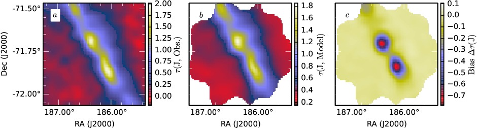
Figure 15: Field G300.86-9.00 as an example of $\tau(J)$ bias maps estimated with simulated NICER observations. The frames show the optical depth derived from actual observations (frame a), average recovered extinction map in simulations (frame b), and the bias as the difference between the output and input maps in the simulation (frame c).

Appendix C Simulated Herschel observations

The estimation of the ${\rm\tau(250\mu m)}$ bias is more uncertain than the estimation of $\tau(J)$ bias. Because of line-of-sight temperature variations, the colour temperature overestimates the mass-averaged dust temperature, which translates into too low estimates of ${\rm\tau(250\mu m)}$. The magnitude of the effect cannot be estimated precisely because the line-of-sight temperature distribution is unknown. Order of magnitude estimates can be obtained with radiative transfer modelling by making assumptions of the radiation field, dust properties, and the cloud structure.

We carried out radiative transfer calculations individually for all the 116 fields. We assumed constant dust properties corresponding to Milky Way dust with a selective extinction of $R_{\rm V}$=5.5 (Draine 2003b). The initial radiation field was assumed to correspond to the Mathis et al. (1983) model of solar neighbourhood. The spectrum of the illuminating radiation has an impact on the temperature contrasts. We have no way to independently determine the shape of the spectrum of the radiation field. However, this typically remains a second-order effect, and the main effect, the level of the radiation field intensity, is part of the modelling. One exception are the possible stars that heat clouds from the inside and may locally have a strong effect. These are considered later in the analysis, but are not part of the simulations.

For each field, we built a model that attempts to reproduce the 250–500 $\mu$m observations of that field. From the background-subtracted surface brightness maps we selected the central $30\arcmin\times 30\arcmin$ area. The model cloud had the same angular dimensions and was discretised onto a $181^{3}$ cell grid. Each cell of the model therefore corresponds to an angular size of 10$\arcsec$ , but the linear scale depends on the distance of the cloud. In the line-of-sight direction we assumed a Gaussian density distribution with a FWHM equal to 25% of the field size. The linear size again depends on the cloud distance because in more distant fields we are also probably concerned with larger structures. In the line-of-sight direction the density peak is always in the central plane of the model cube. This increases mutual shadowing of dense regions, which in reality can reside at different distances and increases the temperature contrasts in the model. On the other hand, for a field at 200 pc distance, the selected line-of-sight FWHM extent is $\sim$0.4 pc, which is larger than the size of typical cores. Therefore, it is difficult to say whether the selection of this particular line-of-sight density profile leads to an over- or underestimation of the final ${\rm\tau(250\mu m)}$ bias. These are usually second-order effects (Juvela et al. 2013) except for very dense clumps that can remain practically invisible in $\tau(J)$ maps as well.

We carried out radiative transfer calculations to produce synthetic surface brightness maps at Herschel wavelengths that were then convolved to the resolution of the observations. The ratio of observed and modelled 350 $\mu$m maps was used to adjust the column densities, applying the same multiplicative factor to all cells along the same line-of-sight. The intensity of the external radiation field was scaled based on the ratios between the observed and modelled 250 $\mu$m and 500 $\mu$m surface brightness. The aim is to also reproduce the average shape of the spectra. The full procedure was iterated until the model matched the observed 350 $\mu$m map at $\sim$1% accuracy and the average ratio 250 $\mu$m/500 $\mu$m were correct within the same tolerance.

The final model takes into account the range of column density, the morphology, and the radiation field intensity of a field. It is not necessarily a perfect match to all surface brightness maps, but is a good facsimile of the pixel-by-pixel column density structure. We analysed the synthetic surface brightness maps as in Sect. 2.2.3. The comparison of the obtained ${\rm\tau(250\mu m)}$ estimates and the true values known for the model cloud gives a $30\arcmin\times 30\arcmin$ map of the ${\rm\tau(250\mu m)}$ bias (resolution 40$\arcsec$). The remaining border areas usually have a low column density and therefore low bias. However, to extend bias estimates over the whole map area, we assigned values calculated using the average bias vs. column density relation estimated from central $30\arcmin\times 30\arcmin$ area to the remaining pixels.

Figure 16 shows one example, the surface brightness maps produced by the model and the bias in the ${\rm\tau(250\mu m)}$ values estimated from these synthetic observations.

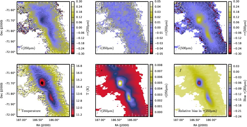
Figure 16: Field G300.86-9.00 as an example of the ${\rm\tau(250\mu m)}$ bias estimation with radiative transfer modelling. The upper row shows the relative error between the model predicted surface brightness and the observations at 250 $\mu$m, 350 $\mu$m, and 500 $\mu$m. The lower frames show the colour temperature and ${\rm\tau(250\mu m)}$ maps calculated from the synthetic observations and the relative bias in ${\rm\tau(250\mu m)}$ obtained by comparison with the actual ${\rm\tau(250\mu m)}$ values in the model.

Appendix D Additional checks of correlations between ${\rm\tau(250\mu m)}$ and $\tau(J)$

In addition to the factors examined in Sect. 2.4, we checked the importance of two additional factors, the technical implementation of the least-squares fits, and the importance of internally heated regions.

The total least-squares fits of Sect. 2.4 used the formal error estimates of $\tau(J)$ and ${\rm\tau(250\mu m)}$. The former were obtained from NICER routine, the latter were estimated with MCMC calculations starting with the assumption of 7% (SPIRE) or 15% (PACS) relative errors in the surface brightness data. If the correlation is poor, the estimated slope becomes sensitive to the error estimates. For example, if the true errors of ${\rm\tau(250\mu m)}$ were much larger, for example because of some artefacts in map making, the use of too low error estimates would increase the slope estimates. We checked this by repeating the analysis using twice the original ${\rm\tau(250\mu m)}$ error estimates. In an extreme case, we can ignore the error estimates altogether and perform unweighted least-squares fits. Based on the error estimates used, the true relative uncertainty is significantly larger in $\tau(J)$ than in ${\rm\tau(250\mu m)}$. Therefore, the unweighted least-squares fit probably underestimates the true slope.

The third test concerns the internally heated regions in which because of strong temperature variations combined with compact, high column density clumps, both optical depth estimates are particularly uncertain. Furthermore, the estimates of ${\rm\tau(250\mu m)}$ bias are probably incorrect in the same areas. This is caused by two factors. First, without the internal heating source, the models are unable to produce sufficient surface brightness values and result in very high column densities and thus high estimates of the bias (Juvela et al. 2013). Second, in the real clump the internal heating may help to decrease the actual bias if the clump centre remains warm instead of being too cold to be registered in Herschel bands (Malinen et al. 2011). We repeated the analysis of Sect. 2.4 by masking warm regions. We first masked all pixels for which the dust colour temperature was higher than 20 K. The mask was then extended to cover areas in which after convolution to 180$\arcsec$ resolution, the influence of the $T>20$ K region was more than 10% of the convolved value.

Figure 17 compares the result with the bias-corrected results already shown in Fig. 4. It shows that the shape of the distribution is not sensitive to the fitting procedure, nor is it significantly affected by the warm regions.

Figure 17: Comparison of $\Delta\tau(250\mu{\rm m})$/$\Delta\tau(J)$ bias-corrected distributions. In addition to the default case, derived distributions are shown for tests with larger ${\rm\tau(250\mu m)}$ error estimates, normal unweighted least squares, and fits excluding data affected by regions with dust temperatures exceeding 20 K.

Appendix E Maps of $\tau(250\mu{\rm m})/\tau(J)$ ratio

In the least-squares fits of Sect. 3.4, the interesting parameters, $k$ and $C$ were independent of additive errors in the correlated quantities. The highest $\tau(J)$ points were particularly important, both visually and regarding the fitted parameters. As mentioned in Sect. 3.5, we also calculated maps of the $\tau(250\mu{\rm m})/\tau(J)$ ratio. Because the column densities are typically low over most of the mapped area, the visual appearance of the maps is dominated by regions with low $\tau(250\mu{\rm m})$ and $\tau(J)$ values where, by definition, the results become sensitive to any zero-point mismatch.

The maps were calculated by first correcting the $\tau(250\mu{\rm m})$ and $\tau(J)$ maps for the bias that was estimated with modelling (see Sect. B and Sect. C). The maps of $\tau(250\mu{\rm m})$ were then convolved to the resolution of the $\tau(J)$ map. A 2$\arcmin$ wide region near the Herschel map borders was masked because the convolved values would be affected by data outside our map coverage. Before calculating the ratio $\tau(250\mu{\rm m})/\tau(J)$, we subtracted from both quantities the values in the reference regions that are listed in Table LABEL:table:fields. A typical diameter of these reference areas is $\sim 6\arcmin$. For $\tau(250\mu{\rm m})$ the statistical error of the reference value is very small. The true uncertainty of the remaining $\tau(250\mu{\rm m})$ is completely dominated by systematic errors. Because the main purpose of the ratio maps is to determine variations in the $\tau(250\mu{\rm m})/\tau(J)$ ratio, we are not very concerned with multiplicative errors.

We expect the statistical errors to be more significant in $\tau(J)$ and, because the variable is in the denominator, we need to mask areas with a low SN of $\tau(J)$ . NICER has provided error maps for $\tau(J),$ but here we estimated the uncertainty using the following procedure: We took the data plotted in Fig. 8, selected 20% of the lowest $\tau(J)$ points, and subtracted from them the prediction of the non-linear fit (red line in Fig. 8). The uncertainty of the reference value, $\Delta\tau(J)$, was calculated as the standard deviation of the residuals, scaled by the ratio of (90$\arcsec$)² and the area of the reference region. This should be a very conservative estimate because it assumes that in Fig. 8 the scatter would be due to $\tau(J)$ errors alone.

The results are shown in Fig. 18. The first frames show the $\tau(250\mu{\rm m})$ maps, the contours indicating the region with a SN of each parameter higher than one. The second frames show the calculated maps of $\tau(250\mu{\rm m})/\tau(J)$. The regions where either parameter falls below SN=0.5 were masked. The remaining frames show the extreme cases corresponding to $\tau(J)\pm\Delta\tau(J)$ and $\tau(250\mu{\rm m})\pm\delta\tau(250\mu{\rm m})$, where $\delta\tau(250\mu{\rm m})$ is the estimated error map (see Sect. 2.2.3).

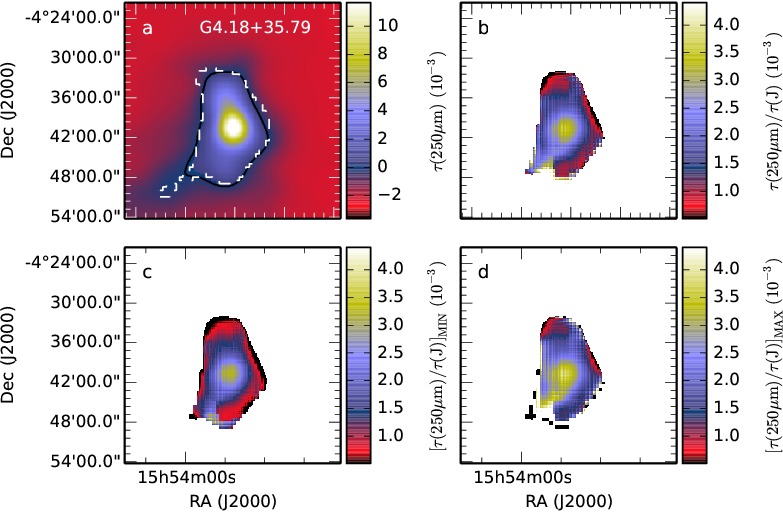
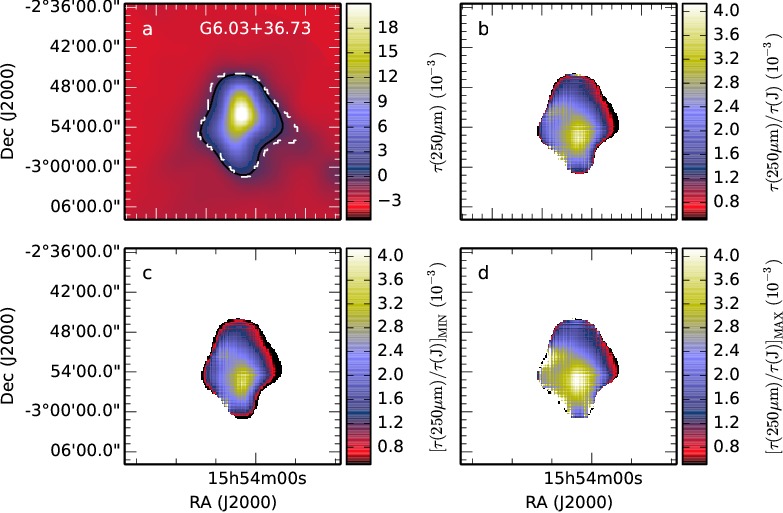
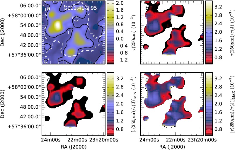
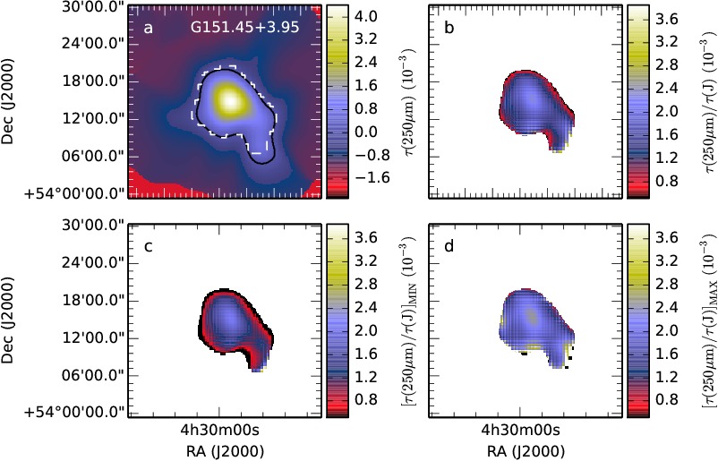
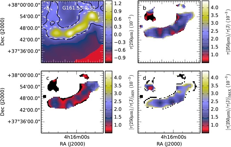
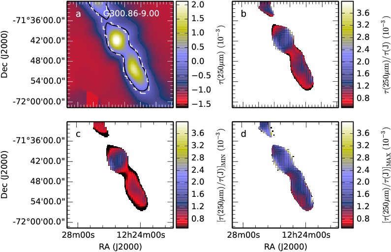
Figure 18: Maps of $\tau(250\mu{\rm m})/\tau(J)$ for the selected fields. The upper frames show $\tau(250\mu{\rm m})$ (frame a) and the ratio $\tau(250\mu{\rm m})/\tau(J)$. The lower frames show the lower (frame c) and upper (frame d) limits of $\tau(250\mu{\rm m})/\tau(J)$ calculated as $(\tau(250\mu{\rm m})+\delta\tau(250\mu{\rm m}))/(\tau(J)-\Delta\tau(J))$ and $(\tau(250\mu{\rm m})-\delta\tau(250\mu{\rm m}))/(\tau(J)+\Delta\tau(J))$ where $\delta\tau(250\mu{\rm m})$ is the error map of $\tau(250\mu{\rm m})$ and $\Delta\tau(J)$ is the estimated uncertainty of the $\tau(J)$ zero point. The areas in which the SN of either variable drops below 0.5 have been masked. In the first frame, the black contour corresponds to $\tau(250\mu{\rm m})=\delta\tau(250\mu{\rm m})$ and the dashed white contour to $\tau(J)=\Delta\tau(J)$.

Table 3: Coordinates and radii of the reference regions used to calculate the near-infrared optical depth maps. The last column lists the id numbers of the Herschel fields themselves.

Field	Reference area		Radius	Herschel Observation IDs
	RA(2000)	DEC(2000)	($\arcmin$)
G0.02+18.02	16 43 59.5	-18 29 20.4	16.8	1342227737, 1342216067, 1342216066
G0.49+11.38	17 01 01.2	-21 23 27.6	10.1	1342227645, 1342216500, 1342216499
G1.94+6.07	17 26 46.8	-23 17 09.6	13.7	1342216944, 1342216588, 1342216587
G2.83+21.91	16 30 59.3	-13 27 46.8	9.6	1342227646, 1342227040, 1342227039
G3.08+9.38	17 18 49.9	-20 40 01.2	14.8	1342252016, 1342252015, 1342251955
G3.72+21.02	16 43 08.9	-13 19 37.2	7.7	1342227647, 1342216502, 1342216501
G4.18+35.79	15 50 46.1	-05 04 37.2	18.8	1342215385, 1342215384, 1342213473
G6.03+36.73	15 56 12.2	-02 02 45.6	10.0	1342204167, 1342204166, 1342203075
G9.45+18.85	17 03 07.7	-10 09 54.0	18.0	1342227648, 1342216504, 1342216503
G10.20+2.39	17 56 04.1	-18 09 07.2	12.1	1342217762, 1342217761, 1342216945
G20.72+7.07	18 02 13.7	-07 34 51.6	10.0	1342216948, 1342216592, 1342216591
G21.26+12.11	17 43 37.9	-03 47 27.6	11.3	1342216949, 1342216590, 1342216589
G24.40+4.68	18 16 02.4	-04 43 19.2	10.9	1342217409, 1342217408, 1342216950
G25.86+6.22	18 18 31.7	-03 17 56.4	11.3	1342217772, 1342217771, 1342216951
G26.34+8.65	18 05 08.9	-01 01 22.8	8.4	1342216952, 1342216594, 1342216593
G37.49+3.03	18 46 05.3	+05 53 42.0	17.7	1342219075, 1342219074, 1342216953
G37.91+2.18	18 49 47.3	+06 09 46.8	16.0	1342229180, 1342219077, 1342219076
G39.65+1.75	18 53 57.8	+07 30 46.8	15.1	1342219633, 1342219079, 1342219078
G62.16-2.92	20 02 27.4	+23 30 36.0	14.9	1342219986, 1342219043, 1342219042
G69.57-1.74	20 15 55.7	+30 40 19.2	14.2	1342220090, 1342220089, 1342219988
G70.10-1.69	20 17 18.0	+31 06 46.8	17.2	1342220092, 1342220091, 1342219987
G71.27-11.32	20 56 03.6	+27 36 25.2	15.0	1342244225, 1342244224, 1342244143
G82.65-2.00	20 57 19.2	+40 46 30.0	11.2	1342222137, 1342221287, 1342221286, 1342219611
G86.97-4.06	21 17 01.4	+42 51 00.0	14.7	1342222116, 1342220280, 1342220279, 1342219610
G89.65-7.02	21 42 49.9	+44 06 32.4	9.1	1342220078, 1342220077, 1342213455
G91.09-39.46	23 14 05.0	+17 15 18.0	10.9	1342221461, 1342221285, 1342221284
G92.04+3.93	20 57 44.9	+53 18 28.8	12.8	1342220862, 1342219031, 1342219030
G92.63-10.43	22 03 29.5	+41 39 25.2	7.4	1342220869, 1342220080, 1342220079
G93.21+9.55	20 31 49.7	+57 36 39.6	18.2	1342220821, 1342220820, 1342213457
G94.15+6.50	20 53 42.5	+56 08 31.2	12.9	1342220553, 1342220552, 1342213456
G95.76+8.17	20 50 34.3	+59 01 55.2	8.3	1342244196, 1342243763, 1342243762
G98.00+8.75	21 07 10.8	+59 13 26.4	15.1	1342220551, 1342220550, 1342220525
G105.57+10.39	21 33 44.9	+67 18 28.8	13.7	1342219970, 1342220819, 1342220818
G107.20+5.52	22 13 59.8	+63 38 09.6	11.7	1342187332, 1342187331
G108.28+16.68	21 07 11.8	+72 31 48.0	13.5	1342216072, 1342216071, 1342213452
G109.18-37.59	00 07 23.0	+24 49 22.8	9.0	1342213511, 1342213510, 1342213494
G109.80+2.70	22 49 03.8	+63 14 56.4	16.5	1342187655, 1342187009, 1342187008, 1342187007
G110.62-12.49	23 41 20.9	+47 50 16.8	19.0	1342222136, 1342222110, 1342222109
G110.89-2.78	23 17 37.7	+57 17 45.6	13.0	1342223343, 1342223342, 1342213453
G110.80+14.16	21 49 39.1	+73 23 02.4	12.4	1342220622, 1342220817, 1342220816
G111.41-2.95	23 16 59.8	+57 02 52.8	13.0	1342223341, 1342223340, 1342213454
G115.93+9.47	23 20 49.2	+72 01 12.0	8.8	1342222598, 1342220666, 1342220665
G116.08-2.40	00 01 23.8	+58 57 28.8	16.6	1342222599, 1342222158, 1342222157
G126.24-5.52	01 21 49.9	+57 04 19.2	10.9	1342224972, 1342216074, 1342216073
G126.63+24.55	04 04 11.0	+84 55 55.2	8.6	1342243735, 1342243734, 1342219426, 1342219425,
				1342219424, 1342199364
G127.79+2.66	01 44 44.9	+65 20 38.4	17.2	1342216512, 1342216511, 1342203610
G128.78-69.46	00 56 41.0	-06 16 12.0	18.2	1342246680, 1342246679, 1342246579
G130.37+11.26	02 33 16.1	+71 50 20.4	9.8	1342218719, 1342218718, 1342216918
G130.42-47.07	01 12 09.8	+14 48 43.2	19.2	1342213525, 1342213524, 1342213486
G131.65+9.75	02 36 24.2	+71 39 21.6	9.5	1342243761, 1342243760, 1342223882, 1342218640,
				1342203609
G132.12+8.95	02 43 03.4	+70 37 44.4	11.4	1342223881, 1342223880, 1342216919
G139.60-3.06	02 47 26.6	+54 55 48.0	16.5	1342226625, 1342216414, 1342216413
G141.25+34.37	08 37 44.9	+73 19 22.8	13.3	1342244197, 1342243739, 1342243738
G149.67+3.56	04 15 01.4	+55 59 38.4	14.1	1342217533, 1342217532, 1342216920
G150.47+3.93	04 22 01.2	+55 45 36.0	17.1	1342217531, 1342217530, 1342214702
G151.45+3.95	04 31 30.5	+53 51 28.8	9.9	1342205043, 1342205042, 1342203607
G154.08+5.23	04 52 23.5	+53 47 24.0	18.1	1342217529, 1342217528, 1342216921
G155.80-14.24	03 40 03.4	+38 29 06.0	13.0	1342226626, 1342224781, 1342224780
G157.08-8.68	04 02 21.6	+42 01 15.6	13.1	1342216416, 1342216415, 1342203615
G157.92-2.28	04 28 53.0	+44 30 25.2	13.7	1342217527, 1342217526, 1342216923
G159.23-34.51	02 59 58.6	+19 12 03.6	13.8	1342239264, 1342239263
G159.12-14.30	03 46 43.0	+34 50 09.6	7.8	1342226627, 1342216419, 1342216418
G159.34+11.21	05 45 49.0	+51 29 31.2	18.6	1342218721, 1342218720, 1342216922
G161.55-9.30	04 12 05.5	+37 11 20.4	11.5	1342205045, 1342205044, 1342203616
G163.82-8.44	04 23 32.6	+36 22 48.0	16.7	1342205048, 1342205047
G164.71-5.64	04 43 22.8	+38 52 48.0	14.5	1342217525, 1342217524, 1342216925
G167.20-8.69	04 34 25.9	+34 10 44.4	6.6	1342217392, 1342217391, 1342216926
G168.85-10.19	04 33 29.5	+31 49 19.2	14.1	1342217523, 1342217522, 1342214701
G171.35-38.28	03 19 13.7	+09 39 25.2	12.8	1342224970, 1342224215, 1342224214
G173.43-5.44	05 07 51.4	+30 37 55.2	17.3	1342217507, 1342217506, 1342216927
G174.22+2.58	05 42 31.9	+34 22 48.0	9.9	1342244179, 1342243759, 1342243758
G176.27-2.09	05 24 21.8	+30 08 06.0	10.3	1342205197, 1342205196, 1342203617
G181.84-18.46	04 47 25.7	+16 18 21.6	10.3	1342217469, 1342217468, 1342203625
G188.24-12.97	05 14 20.9	+14 06 54.0	11.9	1342217455, 1342217454, 1342214700
G189.51-10.41	05 28 18.5	+15 00 07.2	10.9	1342217457, 1342217456, 1342216930
G195.74-2.29	06 13 50.2	+14 48 46.8	17.9	1342219409, 1342219408, 1342216931
G198.58-9.10	05 55 25.0	+08 15 57.6	17.9	1342218702, 1342218701, 1342216932
G202.23-3.38	06 18 57.4	+07 14 02.4	10.2	1342218773, 1342218772, 1342216933
G202.02+2.85	06 42 51.8	+11 30 43.2	12.2	1342228372, 1342228371, 1342228342
G203.42-8.29	06 07 25.2	+05 00 18.0	12.6	1342218777, 1342218776, 1342216935
G205.06-6.04	06 19 59.0	+04 49 15.6	7.6	1342218775, 1342218774, 1342216934
G206.33-25.94	05 04 09.1	-05 37 58.8	9.3	1342249237
G210.90-36.55	04 31 38.4	-13 23 34.8	9.7	1342225213, 1342225212, 1342216940
G212.07-15.21	05 59 01.9	-05 58 30.0	14.0	1342218783, 1342218782, 1342216936
G215.37-3.04	06 44 21.4	-04 16 37.2	15.7	1342219957, 1342219405, 1342219404
G215.44-16.38	05 59 46.6	-08 52 40.8	19.9	1342204306, 1342204305, 1342203631
G216.76-2.58	06 45 47.8	-05 23 56.4	12.0	1342219956, 1342219407, 1342219406
G218.06+2.12	07 11 45.8	-02 43 48.0	8.5	1342219958, 1342220785, 1342220784
G219.36-9.71	06 28 11.3	-09 30 07.2	15.6	1342227708, 1342219403, 1342219402
G219.29-9.25	06 28 20.9	-09 27 43.2	16.5	1342227707, 1342219401, 1342219400
G227.95-2.98	07 04 29.5	-15 27 39.6	10.9	1342219982, 1342220901, 1342220900
G247.55-12.27	07 13 20.6	-36 48 00.0	12.7	1342222831, 1342220781, 1342220780
G253.71+1.93	08 25 07.0	-33 44 45.6	10.8	1342222828, 1342220783, 1342220782
G255.33-4.88	07 58 19.9	-39 40 51.6	16.7	1342222830, 1342220779, 1342220778
G258.90-4.10	08 10 17.0	-42 19 15.6	10.6	1342222896, 1342220777, 1342220776
G265.04+6.08	09 21 18.7	-40 14 38.4	7.8	1342222845, 1342220309, 1342220308
G265.60-5.82	08 32 48.5	-47 47 06.0	12.0	1342222829, 1342220775, 1342220774
G268.21+2.02	09 17 09.8	-44 53 49.2	17.7	1342222827, 1342221275, 1342221274
G271.06+4.84	09 41 12.0	-45 28 51.6	9.9	1342222895, 1342221270, 1342221269
G271.51+5.14	09 44 13.9	-45 54 39.6	10.2	1342222894, 1342221268, 1342221267
G276.78+1.75	09 54 27.1	-51 06 21.6	9.8	1342198593, 1342198592
G298.31-13.05	11 26 36.0	-75 02 52.8	11.7	1342223601, 1342223600, 1342216941
G299.57+5.61	12 22 23.3	-56 28 33.6	23.5	1342223605, 1342223604, 1342223259
G300.61-3.13	12 27 23.0	-66 32 20.4	15.1	1342223603, 1342223602, 1342213480
G300.86-9.00	12 14 18.7	-72 08 02.4	11.4	1342188162, 1342188101, 1342188100, 1342188099
G315.88-21.44	17 06 03.4	-77 16 37.2	14.6	1342218738, 1342218737, 1342216942
G320.84+5.09	14 55 25.2	-52 38 56.4	13.2	1342227725, 1342215598, 1342215597
G325.54+5.82	15 16 29.0	-49 30 54.0	9.8	1342227693, 1342225000, 1342224999
G332.70+6.77	15 47 46.1	-44 43 04.8	15.5	1342227692, 1342226700, 1342226699
G334.65+2.67	16 10 07.0	-46 25 26.4	13.5	1342216490, 1342216489, 1342214758
G339.22-6.02	17 15 55.9	-50 25 01.2	9.3	1342216582, 1342216581, 1342214757
G341.18+6.51	16 21 30.2	-39 15 07.2	9.4	1342227691, 1342216492, 1342216491
G343.64-2.31	17 14 32.4	-44 28 40.8	17.3	1342216943, 1342216584, 1342216583
G344.77+7.58	16 29 49.0	-37 18 21.6	13.7	1342227690, 1342216496, 1342216495
G345.39-3.97	17 26 34.1	-43 44 13.2	20.6	1342252027, 1342251963
G358.96+36.75	15 36 34.1	-07 12 54.0	12.2	1342204169, 1342204168, 1342202205

Table 3: continued.