An equilibrium model for spot and forward prices of commoditiest

Abstract

We consider a market model that consists of financial investors and producers of a commodity. Producers optionally store some production for future sale and go short on forward contracts to hedge the uncertainty of the future commodity price. Financial investors take positions in these contracts in order to diversify their portfolios. The spot and forward equilibrium commodity prices are endogenously derived as the outcome of the interaction between producers and investors. Assuming that both are utility maximizers, we first prove the existence of an equilibrium in an abstract setting. Then, in a framework where the consumers’ demand and the exogenously priced financial market are correlated, we provide semi-explicit expressions for the equilibrium prices and analyze their dependence on the model parameters. The model can explain why increased investors’ participation in forward commodity markets and higher correlation between the commodity and the stock market could result in higher spot prices and lower forward premia.

Commodities, equilibrium, spot and forward prices, forward premium, stock and commodity market correlation.

Q02, G13, G11, C62 91B50, 90B05

1 Introduction

Since the early 2000s, the futures and forward contracts written on commodities have been a widely popular investment asset class for many financial institutions. As indicatively reported in [17], the value of index-related futures’ holdings in commodities grew from $15 billion in 2003 to more than $200 billion in 2008. This significant inflow of funds has coincided, up to 2008, with a steep increase in the spot and futures prices of the majority of commodities, especially the ones included in popular commodity indices. The comovement of amounts invested in commodity-linked securities and the prices of the associated commodities continued even during the prices’ bust in 2008 and their recovery which started in 2009; see e.g. the empirical studies presented in Singleton [57], Tang and Xiong [60] and Buyuksahin and Robe [10]. Furthermore, several statistical studies have found that the correlation between commodity prices and the stock market has grown during the last years. As an example, [10] argues that the correlation of the U.S. stock market (weekly) returns and the returns of the GSCI commodity indices varies from -38% to 40% depending on the period, and stays positive and away from zero after 2009; further statistical evidence on the increased correlation are given in [60], [57] and in Singleton and Thorp [56]. Therefore, the investment strategies of financial institutions on stock and commodity markets should be considered in the same optimization problem and not independently.

The booms and busts of the prices of major commodities during the last decade has naturally captured the interest of the academic community. The main question addressed is whether the behavior of commodities’ prices is caused by the (enhanced by the financialization) positions of speculators or by the fluctuations of fundamental economic factors (i.e. increased demand and weakend supply). Even though there exist several empirical studies, the theoretical approaches that link spot and forward prices of commodities with the rest of the investment assets are scarce.

The main goal of this paper, is to establish an equilibrium model that allows to endogenously derive both the spot and the forward price of a commodity, and is flexible and general enough to include not only the randomness of the commodity demand and the commodity holders’ storage option, but also risk averse agents and correlation between the stock and the commodity market. In our model, equilibrium commodity prices are formed as the outcome of the interaction between market participants, and simultaneously clear out the spot and the forward market. The forces that lead to the market equilibrium are the producers’ goal to maximize their spot revenues and optimally hedge the risk of the future commodity price, and the investors’ goal to achieve an optimal portfolio strategy that, besides the stock market, includes also a position in the commodity’s forward contracts. The model offers new insights on how specific model inputs, such as the agents’ risk aversion, the correlation of the stock and commodity market and the uncertainty of the future commodity price, influence the equilibrium prices and the related risk premia.

1.1 Model description

We consider a model of two points in time: the initial one and a given (short-term) future horizon $T$. We assume that the main market participants are the representative agents of the commodity’s holders/suppliers and the financial investors/speculators, who shall hereafter be called producers and investors respectively.

The producers’ source of income are the revenues from spot and future sales. While the commodity spot price could be determined by the spot commodity demand function, the future price is subject to demand shocks. Assuming that producers are risk averse, their goal is not only to maximize their spot revenues, but also to reduce their risk exposure to the future commodity price by maximizing their expected utility. If the production schedule at the initial and future time is a predetermined pair of units, producers have two decisions to make: what amount of the production to supply in the spot market (inventory management) and what position to take in the forward contract (hedging strategy). Provided they know the demand function of the commodity’s consumers at the initial time, they can determine the commodity spot price by choosing the amount of the inventory they will hold up to the terminal time. However, random demand shocks at time $T$ will shift the whole demand function to lower or higher levels (for instance, in Section 4 we suppose that the random shift of the demand function is driven by a vector of stochastic market factors). Producers hedge the risk which stems from the future time demand function by taking a short position in forward contracts written on the same commodity and with maturity equal to $T$. The fact that the inventory will also be sold at time $T$ makes the forward hedging position even more important for the producers.

The producers’ hedging demand is covered by financial investors, who take the opposite position in the forward commodity contracts and thus share some of the future price uncertainty risk, possibly against a premium. They invest optimally in an exogenously priced stock market and are willing to take the future commodity price risk in order to better diversify their portfolio. Indeed, as mentioned above, the correlation between commodity and stock market indices has been shown to be away from zero. This correlation could be incorporated in a model where the stock market price is driven by the same stochastic factors that drive the evolution of the commodity demand function. Given this correlation, the optimal investment strategy in the stock and the commodity market should be considered in the same optimization problem. As in the producers’ side, we assume that the investors are represented by an agent who is a utility maximizer and whose investment choices are the (possibly dynamic) trading strategy in the stock market and the position in the forward commodity contract.

The optimization choices of both producers and investors clearly depend on the forward commodity price. We define as equilibrium forward price the price that clears the forward market and at which both participants’ expected utilities are maximized. Given the forward price, the producers optimally choose the inventory policy, which in turn gives the initial commodity supply and thus determines the spot price through the initial demand function of the consumers. Therefore, by deriving the equilibrium forward commodity price, the equilibrium spot price as well as the producers’ optimal inventory policy are also endogenously derived in our model.

1.2 Findings and contributions

The main mathematical result of this work is to prove, under CARA preferences and upon some minor technical assumptions, that equilibrium spot and forward commodity prices exist. In this proof, we use standard duality arguments to show that both producers’ and investors’ optimization problems are well-defined and admit finite solutions. The existence of the forward commodity equilibrium price is first proved for every fixed producers’ storage choice. Then, we show that this equilibrium is stable with respect to the storage choice, which in turn guarantees the existence of the commodity market equilibrium. In fact, this stability result is interesting in its own right, since it shows that the market clearing is stable with respect to any control variable which belongs to a closed set of real numbers.

The constructive nature of the aforementioned proof allows us to derive implicit formulas for spot and forward prices, which can be used to investigate how the main model parameters influence the commodity market. We illustrate this using two examples with factors driven by Lévy processes; first a Brownian motion and then a jump-diffusion process. The main results are given below.

Focusing first on the equilibrium spot price, our results imply it is monotonic with respect to the agents’ risk aversion coefficient; it is increasing for producers and decreasing for investors (see Figures 5.1 and 5.2). When producers are more concerned about the commodity future price uncertainty, they increase their position in the forward contract and hence lock the selling price at the terminal time. As long as the hedging position is counterpartied by the investors, high risk averse producers can increase their certain revenues today and at the same time hedge their future price risk. What is very important in this monotonicity is the correlation between the stock market and the demand random shocks. As it is illustrated in Section 5, when correlation is away from zero, the equilibrium spot price is pushed upwards. This is mainly because higher correlation means that investors are able to better hedge their risk exposure in the commodity market by adjusting their investments in the stock market. Hence, they are willing to receive a lower forward premium, thus making hedging cheaper for the producers. In particular, when the investors are more risk averse, they reduce their share in the future commodity price risk; thus, producers cannot hedge their future price risk which forces them to increase their supply in the spot market. Therefore, the spot price is a decreasing function of investors’ risk aversion (all else equal). Also, it follows that the producers’ ability to hedge their risk tends to increase the spot equilibrium prices. Moreover, our model yields that the existence of a forward contract in the commodity market stabilizes spot prices when there is scarcity of the commodity at the terminal time; in particular, the presence of forward contracts increases the current spot and decreases the expected future spot price of the commodity.

The monotonicity of the spot price with respect to risk aversions could also be used to explain how the participation of investors in the commodity forward markets could result in an increase of spot commodity prices. Indeed, under CARA preferences the more investors participate in the market, the higher the aggregate risk tolerance becomes or, equivalently, the lower the representative risk aversion’ coefficient becomes (see, among others, Wilson [61]). As discussed above, this implies higher spot commodity price, a result that is consistent with the observed market data (see e.g. [10] and Henderson et al. [33]). Similarly, we verify that more producers (of the same total production) implies lower spot price.

Besides equilibrium commodity spot prices, our model allows to endogenously derive quantities that characterize the two major, and not mutually exclusive, theories of forward commodity markets: the theory of storage and the theory of normal backwardation. Based on the ideas introduced in Kaldor [40], Working [62] and Brennan [9], the theory of storage states that the holders of the commodity inventories get an implicit benefit, called convenience yield, which implies the value of the spot commodity consumption. This yield can be approximated by the difference between the spot and the forward price minus the cost of storage. Our equilibrium model verifies that the convenience yield is increasing with respect to the producers’ risk aversion, meaning that the more sensitive about the risk the producers are, the more commodity forward units they hedge depressing the forward price (see Figure 5.6 for the Brownian motion example). A similar increasing relation holds for the investors (these relations, in particular, generalize the results of Proposition 1 in Acharya et al. [1]). However, the convenience yield is not always monotonic with respect to the correlation coefficient. As discussed in Section 4, there are two effects of opposing direction on the convenience yield, one coming from the decrease of the effective investors’ risk aversion and other from the corresponding increase on the spot price. The total effect mainly depends on the level of the agents’ risk aversions and the (uneven) production levels at initial and terminal time (see Figures 5.6 and 5.7).

On the other hand, the theory of normal backwardation (see the seminal works by Keynes [43] and Hicks [34]), states that there is a positive premium required by the investors in order to satisfy the producers’ hedging demand in forward contracts. This premium, usually called forward or insurance premium, is given as the percentage difference between the expected commodity price at maturity and its forward price. As expected, this premium is increasing (decreasing) with respect to investors’ (producers’) risk aversion.

In contrast to the existing literature, our model includes as an input the correlation between the stock market and the commodity demand shock. Several empirical studies have shown that this correlation is indeed non-zero and, as our results demonstrate, it does influence the equilibrium prices heavily. In particular, as it is shown in Section 5, the effective investors’ risk aversion coefficient is decreasing in the presence of non-zero correlation. This simply reflects the fact that higher correlation means better hedging of the forward contract position by trading in the stock market (provided there are no short-selling constraints on the investors’ trading strategies). Hence, non-zero correlation has in principle the same effect on the equilibrium as a decrease in the investors’ risk aversion (see Figures 5.1, 5.2 and 5.5). For instance, higher correlation (in absolute values) means higher spot commodity price, a result that is also consistent with the observed market data (see e.g. [60]). A similar effect is caused by an increased variance of the demand shock, which can be due to the presence of jumps (see Figure 5.5).

1.3 Relation with the existing literature

Equilibrium pricing models in markets that consist of utility maximizing agents have been recently addressed by a number of authors in mathematical finance; see, among others, Anthropelos and Žitković [4], Barrieu and El Karoui [7], Cheridito et al. [15], Filipović and Kupper [25], Horst and Müller [37] and Karatzas et al. [42]. The results in this literature however do not cover the case of commodity forward contracts, not only because a commodity has a consumption value which is reflected by the consumers’ demand function, but also due to the producers’ specific storage choice. To the best of our knowledge, this paper is the first to apply a utility maximization criterion for spot and forward equilibrium prices of commodities, while considering also the existence of a correlated stock market.

Theoretical studies of the equilibrium relationship between spot and forward commodity prices go back to Stoll [58], Anderson and Danthine [3] and Hirshleifer [35, 36]. The results of these seminal works are limited regarding the agents’ risk preferences, which are assumed to be mean-variance, while recent extensions of this setting have followed different approaches than ours. For instance in Baker [6], mean-variance optimization problems are imposed in a discrete time dynamic model, where investors are the ones that have the storage option and the consumers (the households) get utility from consumption and the wealth (numéraire units). In Routledge et al. [51] and Pirrong [49], investors are assumed to be risk neutral and without access to other financial markets, while forward prices are simply the expectations of future spot prices. The interaction between the optimal storage and the investors’ optimal position in the forward contract and its effect to spot and forward equilibrium prices are also studied in Ekeland et al. [24]. However, in contrast to our model the investors trade only in forward contracts, while the preferences are mean-variance, which means that they are not monotonic with respect to futures revenues. More recently, endogenous commodity supply under asymmetric information and limited participation has been developed in Leclercq and Praz [48]. Static mean-variance models have been also studied and statistically tested in Acharya et al. [1] and Gorton et al. [30], however neither the investors nor the producers trade in any other market outside of the commodity market. Hence, their theoretical results cover only a very special case of our model, namely, when the stock and the commodity market are uncorrelated and the demand random shift is normally distributed.

The main novelties of our approach compared to the related literature are the consideration of an exogenous stock market available in the investors’ trading set, the risk aversion of the agents’ preferences and the much richer family of processes that model the market factors. Indeed, as has already been discussed, both the correlation between the stock and commodity market and the jump component do influence the equilibrium prices.

This paper is structured as follows: Section 2 sets up the general framework for our equilibrium model. The well-posedness of the agents’ optimization problems and the existence of an equilibrium are proved in Section 3. Section 4 studies a model with continuous trading under Lévy dynamics, where semi-explicit formulas for equilibrium quantities are derived and discussed. Finally, Section 5 focuses on two examples that permit the illustration and a further economic interpretation of the results. Technical proofs of Section 5 are placed in Appendix A.

2 A general framework for commodity prices

We start by describing a general modeling framework where the interaction of market participants determines the spot and forward prices of commodities. The model consists of a pair of representative agents: the producers produce the commodity, supply part of the production at the spot market and store the rest, while they hedge their exposure to price fluctuations using forward contracts on the commodity. The investors invest in financial markets and, in order to diversify their portfolio, they also invest in the commodities forward market. Moreover, the model includes consumers who consume the commodity at the spot market. The goal is to determine the price of the commodity that makes the forward market clear out, assuming that both producers and investors are utility maximizers.

More specifically, the producers produce $\pi_{0}$ units of the commodity at the initial time 0 and $\pi_{T}$ units at the terminal time $T$; both $\pi_{0}$ and $\pi_{T}$ are assumed to be deterministic. They offer $\pi_{0}-\alpha$ units at the spot market at time $0$ and store the rest for time $T$. Furthermore, they hedge their exposure by investing in the forward market. Therefore, their position at time $T$ is

$$\underline{w}(\alpha,h^{p}) =P_{0}(\pi_{0}-\alpha)(1+R)+P_{T}(\pi_{T}+\alpha(1-\varepsilon))+h^{p}(P_{T}-F),$$ (2.1)

where $P_{0}$ and $P_{T}$ denote the spot price at times $0$ and $T$ respectively, $R$ the discretely compounded interest rate, $\varepsilon\in[0,1]$ the cost of storage considered as percentage of the stored units, $F$ the forward price and $h^{p}$ the amount of forward contracts held by the producers. A positive $h^{p}$ indicates a long position in the forward contract, while a negative $h^{p}$ amounts to a short one. The producers’ utility is assumed to be exponential, henceforth their preferences are described by

$$\mathbb{U}_{p}(v)=-\frac{1}{\gamma_{p}}\log\mathbb{E}\left[\mathrm{e}^{-\gamma_{p}v}\right],$$ (2.2)

where $\gamma_{p}>0$. As in Anderson and Danthine [2, 3], their problem is to find an optimal storage strategy $\alpha\in[0,\pi_{0}]$ and an optimal hedging strategy $h^{p}\in\mathbb{R}$ that maximize the utility of their position (2.1). Therefore, their utility maximization problem is

$$\Pi^{p}:=\underset{\alpha\in[0,\pi_{0}],\,h^{p}\in\mathbb{R}}{\sup}\mathbb{U}_{p}\big{(}\underline{w}(\alpha,h^{p})\big{)}.$$ (2.3)

The spot price of the commodity is the price at which the consumers’ demand equals the producers’ supply. The consumers’ demand at the initial time is given by a strictly decreasing and linear function

$$\psi_{0}(x)=\mu-mx,$$ (2.4)

where $\mu\in\mathbb{R}$ and $m\in\mathbb{R}_{+}$, while $x$ denotes the price. The parameter $m$ is a measure of the elasticity of demand for the commodity. The demand at the terminal time is random and depends on the factors driving the commodities market, which are incorporated in a random variable $X$. The demand function at the terminal time is of the form

$$\psi_{T}(x)=\psi_{0}(x)+X.$$ (2.5)

In other words, we assume that the shape and the elasticity of the demand function remain the same, however there is a random shift acting on it. This shift may be, for example, the result of an increase or decrease in the prices of the competitive commodities, of fluctuations in a dominated currency, or of an exogenous increase in the demand for every price level. Since the demand function is linear, the inverse demand function is also linear and equals

$$\phi_{0}(y)=\frac{\mu-y}{m}\quad\text{ and }\quad\phi_{T}(y)=\frac{\mu+X-y}{m}.$$ (2.6)

Henceforth, if the producers store $\alpha$ units at the initial time, the spot price of the commodity, determined by the equilibrium condition between demand and supply, equals

$$P_{0} =\phi_{0}(\pi_{0}-\alpha)=\phi_{0}(\pi_{0})+\frac{\alpha}{m},$$ (2.7)

while the commodity spot price at the terminal time is

$$P_{T} =\phi_{T}\big{(}\pi_{T}+\alpha(1-\varepsilon)\big{)}=\phi_{0}(\pi_{T})-\frac{\alpha(1-\varepsilon)}{m}+\frac{X}{m}.$$ (2.8)

The producers control the spot price by choosing the inventory policy. By storing more commodity units they increase the spot price, but they also increase their exposure to the variation of the future spot price since the stored units will be supplied at the next time period.

The investors take a position $h^{s}$ in the forward contract and invest in an exogenously priced financial market. Their position at time $T$ equals

$$\overline{w}(G,h^{s}) =h^{s}(P_{T}-F)+G,$$ (2.9)

for $G\in\mathcal{G}$, where $\mathcal{G}$ is a set of random variables that models discounted trading outcomes attainable with zero initial wealth. This general formulation allows to consider different scenarios simultaneously.

Example 2.1.

The simplest scenario is $\mathcal{G}=\{0\}$, whence the investors can only invest in the forward contract. Another scenario is to consider an asset price process $S$ and denote by $G(\theta)=\int_{0}^{\cdot}\theta_{u}\mathrm{d}S_{u}$ the gains process for a trading strategy $\theta$. In that case, the set of trading outcomes $\mathcal{G}$ is given by

$$\mathcal{G}=\{G_{T}(\theta):\theta\in\Theta\},$$

for a set $\Theta$ of admissible, self-financing trading strategies. Transaction costs can be easily incorporated as well by setting

$$\mathcal{G}=\{G_{T}(\theta)-k(\theta):\theta\in\Theta\},$$

where $k:\Theta\to\mathbb{R}$ is a concave function.

We assume that the investors’ utility is also exponential with $\gamma_{s}>0$, that is, their preferences are described by

$$\mathbb{U}_{s}(v)=-\frac{1}{\gamma_{s}}\log\mathbb{E}\left[\mathrm{e}^{-\gamma_{s}v}\right],$$ (2.10)

therefore their utility maximization problem reads as

$$\Pi^{s}:=\sup_{h^{s}\in\mathbb{R},\,G\in\mathcal{G}}\mathbb{U}_{s}\big{(}h^{s}(P_{T}-F)+G\big{)}.$$ (2.11)

The maximization problem of both participants depends on the forward price $F$. This price is determined by the equilibrium in the forward market, which is defined below.

Definition 2.2.

A triplet $(\hat{\alpha},\hat{h},\hat{F})$ is called an equilibrium if it satisfies the following conditions:

• Market clearing: the forward market clears out in the sense that

  $$\hat{h}:=h^{p}(\hat{F})=-h^{s}(\hat{F}).$$ (2.12)

• Optimality: the pair $(\hat{\alpha},\hat{h})$ is optimal for the producers’ problem $\Pi^{p}$ and $\hat{h}$ is optimal for the investors’ problem $\Pi^{s}$.

The price $\hat{F}=F(\hat{\alpha})$ is called the equilibrium commodity forward price at maturity $T$. The induced price $\hat{P}_{0}:=P_{0}(\hat{\alpha})$ derived by (2.7) is called the equilibrium commodity spot price at $0$.

Remark 2.3.

The utility maximization problems of both agents are equivalent to risk minimization problems relative to the entropic risk measure; see e.g. Barrieu and El Karoui [7]. The risk measure point of view is more natural for certain agents, such as a corporation managing its risk exposure.

3 Equilibrium in the general framework

The aim of this section is to show that an equilibrium exists in the general modeling framework described above, under mild assumptions on the random variable $X$ and the set of trading outcomes $\mathcal{G}$. Let $(\Omega,{\cal F},\mathbb{P})$ be a probability space where $\mathcal{F}=\mathcal{F}_{T}$. In the sequel all equalities and inequalities between random variables are understood in the $\mathbb{P}$-almost sure sense. The interior and the boundary of a set $K$ are denoted by $K^{\circ}$ and $\partial K$, respectively, and the domain of a function $f$ by $\mathrm{dom}f$.

We denote the set of exponential moments of $X$ by $\mathcal{U}_{X}=\{u\in\mathbb{R}:\mathbb{E}[\mathrm{e}^{uX}]<\infty\}$ and define the cumulant generating function of $X$ by

$$\kappa_{X}(u)=\log\mathbb{E}\left[\mathrm{e}^{uX}\right],\qquad u\in\mathcal{U}_{X}.$$ (3.1)

The following conditions will be used throughout this work:

1. $0\in\mathcal{U}^{\circ}_{X}.$

1. If $\partial\mathcal{U}_{X}=\pm\infty$ then the following limit holds:

   $$\lim_{z\to\pm\infty}\frac{\kappa_{X}(z)}{|z|}=+\infty.$$

The next lemma summarizes some useful properties of the cumulant generating function.

Lemma 3.1.

The cumulant generating function $\kappa_{X}$ is convex and lower semicontinuous.

Proof 3.2.

Convexity follows directly from Hölder’s inequality; for $p,q\in(0,1)$ conjugate, we have that

$$\kappa_{X}(pu+qv) =\log\mathbb{E}\big{[}\mathrm{e}^{puX}\mathrm{e}^{qvX}\big{]}$$

$$\leq\log\big{\{}\big{(}\mathbb{E}\big{[}\mathrm{e}^{uX}]\big{)}^{p}\big{(}\mathbb{E}\big{[}\mathrm{e}^{vX}]\big{)}^{q}\big{\}}=p\kappa_{X}(u)+q\kappa_{X}(v).$$

In order to show lower semicontinuity, consider a sequence $u_{n}\rightarrow u$; then $\mathrm{e}^{u_{n}x}$ is a sequence of positive functions. Applying Fatou’s lemma, we get

$$\liminf_{u_{n}\to u}\kappa_{X}(u_{n}) =\liminf_{u_{n}\to u}\log\mathbb{E}\big{[}\mathrm{e}^{u_{n}X}\big{]}$$

$$\geq\log\mathbb{E}\big{[}\liminf_{u_{n}\to u}\mathrm{e}^{u_{n}X}\big{]}=\kappa_{X}(u).$$

3.1 Producers’ optimization problem

The first step is to consider the producers’ optimization problem and show that it admits a maximizer under mild assumptions. The producers’ position, using the spot market equilibrium conditions (2.7) and (2.8), can be written as

$$\underline{w}(\alpha,h^{p}) =P_{0}(\pi_{0}-\alpha)(1+R)+P_{T}(\pi_{T}+\alpha(1-\varepsilon))+h^{p}(P_{T}-F)$$

$$\stackrel{{\scriptstyle[}}{{\eqref{}}}{eq:fin_{p}rice}]{\eqref{eq:ini_price}}{=}\left(\phi_{0}(\pi_{0})+\frac{\alpha}{m}\right)(\pi_{0}-\alpha)(1+R)-h^{p}F$$

$$\quad+\big{(}\pi_{T}+\alpha(1-\varepsilon)+h^{p}\big{)}\left(\phi_{0}(\pi_{T})-\frac{\alpha(1-\varepsilon)}{m}+\frac{X}{m}\right)$$

$$=:\mathrm{q}(\alpha,h^{p})+\ell(\alpha,h^{p})X,$$ (3.2)

where $\mathrm{q}$ is a quadratic function in $\alpha$ and $h^{p}$ of the form

$$\mathrm{q}(\alpha,h^{p}) =-\alpha^{2}\frac{1+R+(1-\varepsilon)^{2}}{m}+\alpha\frac{2(1+R)\pi_{0}-2(1-\varepsilon)\pi_{T}-(R+\varepsilon)\mu}{m}$$

$$\quad-\alpha h^{p}\frac{1-\varepsilon}{m}-h^{p}\left(F-\frac{\mu-\pi_{T}}{m}\right)+\pi_{T}\phi_{0}(\pi_{T})+\pi_{0}\phi_{0}(\pi_{0})(1+R),$$ (3.3)

while $\ell$ is a bilinear function in $\alpha$ and $h^{p}$ given by

$$\ell(\alpha,h^{p})=\frac{\alpha(1-\varepsilon)+h^{p}+\pi_{T}}{m}.$$ (3.4)

Using the translation invariance of the exponential utility function, the producers’ utility takes the form

$$\mathbb{U}_{p}\big{(}\underline{w}(\alpha,h^{p})\big{)} =-\frac{1}{\gamma_{p}}\log{\mathbb{E}}\Big{[}\exp\Big{(}-\gamma_{p}\big{\{}\mathrm{q}(\alpha,h^{p})+\ell(\alpha,h^{p})X\big{\}}\Big{)}\Big{]}$$

$$=\mathrm{q}(\alpha,h^{p})-\frac{1}{\gamma_{p}}\log{\mathbb{E}}\Big{[}\exp\Big{(}-\gamma_{p}\ell(\alpha,h^{p})X\Big{)}\Big{]}$$

$$=\mathrm{q}(\alpha,h^{p})-\frac{1}{\gamma_{p}}\kappa_{X}\big{(}-\gamma_{p}\ell(\alpha,h^{p})\big{)},$$ (3.5)

assuming that $-\gamma_{p}\ell(\alpha,h^{p})\in\mathcal{U}_{X}$. In the sequel, we will work with the extended producers’ utility $\widetilde{\mathbb{U}}_{p}(\underline{w}(\alpha,h^{p}))$ which is defined as follows:

$$\widetilde{\mathbb{U}}_{p}\big{(}\underline{w}(\alpha,h^{p})\big{)}=\left\{\begin{array}[]{ll}\mathbb{U}_{p}\big{(}\underline{w}(\alpha,h^{p})\big{)},&\text{if }(\alpha,h^{p})\in\widetilde{\mathcal{U}}_{X},\\ -\infty,&\text{otherwise},\\ \end{array}\right.$$ (3.8)

where $\widetilde{\mathcal{U}}_{X}=\left\{(x_{1},x_{2})\in\mathbb{R}^{2}:-\gamma_{p}\ell(x_{1},x_{2})\in\mathcal{U}_{X}\right\}$. The producers’ optimization problem (2.3) can then be written as follows

$$\Pi^{p} =\underset{\alpha\in[0,\pi_{0}]}{\sup}\underset{h^{p}\in\mathbb{R}}{\sup}\widetilde{\mathbb{U}}_{p}\big{(}\underline{w}(\alpha,h^{p})\big{)}$$

$$=\underset{\alpha\in[0,\pi_{0}]}{\sup}\underset{h^{p}\in\mathbb{R}}{\sup}\{u_{p}(\alpha,h^{p})-h^{p}F\}=\underset{\alpha\in[0,\pi_{0}]}{\sup}\{-u_{p}^{*}(\alpha,F)\},$$ (3.9)

where

$$u_{p}(\alpha,h^{p})=\left\{\begin{array}[]{ll}\mathrm{q}(\alpha,0)-\frac{1}{\gamma_{p}}\kappa_{X}\big{(}-\gamma_{p}\ell(\alpha,h^{p})\big{)}-h^{p}\ell(\alpha,-\mu),&\hbox{if $(\alpha,h^{p})\in\widetilde{\mathcal{U}}_{X}$,}\\ -\infty,&\hbox{otherwise,}\\ \end{array}\right.$$ (3.12)

while $u_{p}^{*}(\alpha,\cdot)$ denotes the conjugate function of $u_{p}(\alpha,\cdot)$, for every $\alpha\in[0,\pi_{0}]$.

Proposition 3.3.

Assume that conditions $(\mathbb{EM})$ and $(\mathbb{COE})$ hold. Then, for every $F\in\mathbb{R}$ there exists a maximizer $(\hat{\alpha},\hat{h}^{p})$ for the producers’ problem $\Pi^{p}$ such that $(\hat{\alpha},\hat{h}^{p})\in\widetilde{\mathcal{U}}_{X}$.

Proof 3.4.

The function $\widetilde{\mathbb{U}}_{p}(\underline{w}(\alpha,h^{p}))$ in (3.1) is upper semicontinuous, strictly concave in $\alpha$ and concave in $h^{p}$, since $\mathrm{q}$ is quadratic, $\ell$ is linear and $\kappa_{X}$ is convex and lower semicontinuous in its arguments; see Lemma 3.1 and (3.1)–(3.4). Observe that $\alpha$ takes values in a bounded set. If the set $\mathcal{U}_{X}$ is also bounded, then the existence of a maximizer follows by the concavity and the upper semicontinuity of $\mathbb{U}_{p}(\underline{w}(a,h^{p}))$. Otherwise, if $\mathcal{U}_{X}$ is unbounded, using Assumption $(\mathbb{COE})$, the linearity of $\ell$ in $\alpha$ and that $\alpha$ belongs to a bounded set, we get that

$$\lim_{h^{p}\to\pm\infty}\inf_{\alpha\in[0,\pi_{0}]}\frac{\kappa_{X}\big{(}-\gamma_{p}\ell(\alpha,h^{p})\big{)}}{|h^{p}|}=+\infty.$$ (3.13)

Therefore, $\mathbb{U}_{p}(\underline{w}(\alpha,h^{p}))$ is coercive in $h^{p}$ resulting in the existence of a maximizer. Finally, if $(\hat{\alpha},\hat{h}^{p})$ does not belong to $\widetilde{\mathcal{U}}_{X}$, then the utility of the producers is not maximized, see (3.8).

Corollary 3.5.

Assume that conditions $(\mathbb{EM})$ and $(\mathbb{COE})$ hold. Then, the function $u_{p}(\alpha,\cdot)$ is concave and upper semicontinuous for every $\alpha\in[0,\pi_{0}]$. In addition, it is coercive uniformly in $\alpha$, that is

$$\lim_{h^{p}\to\pm\infty}\sup_{\alpha\in[0,\pi_{0}]}\frac{u_{p}(\alpha,h^{p})}{|h^{p}|}=-\infty.$$ (3.14)

Remark 3.6.

It follows from (3.1), that small production at time $T$ raises the producers’ desire to store, even when the future demand function is deterministic. This occurs because a possible scarcity of the commodity at time $T$ would result in higher future spot prices, hence producers would be better off storing some production and selling it at time $T$. On the other hand, higher future production decreases the optimal storage choice. Hence, the producers’ desire to balance uneven productions is an important feature that influences the optimal storage choice.

3.2 Investors’ optimization problem

The second step is to analyze the structure and properties of the investors’ optimization problem. Although we cannot prove the existence of a maximizer at this level of generality, the results we obtain are sufficient to show the existence of an equilibrium in the next subsection.

Let $\mathbb{Q}$ be a probability measure on $(\Omega,\mathcal{F})$. The relative entropy $\mathcal{H}(\mathbb{Q}|\mathbb{P})$ of $\mathbb{Q}$ with respect to $\mathbb{P}$ is defined by

$$\mathcal{H}({\mathbb{Q}}|{\mathbb{P}})=\left\{\begin{array}[]{ll}{\mathbb{E}}_{{\mathbb{Q}}}\big{[}\ln\big{(}\frac{\mathrm{d}{\mathbb{Q}}}{\mathrm{d}{\mathbb{P}}}\big{)}\big{]},&\text{if }{\mathbb{Q}}\ll{\mathbb{P}},\\ +\infty,&\text{otherwise}.\\ \end{array}\right.$$

Given $\alpha\in[0,\pi_{0}]$, the spot price of the commodity $P_{T}=P_{T}(\alpha)$ is provided by (2.8). Define the function

$$u_{s}(\alpha,h^{s}):=\sup_{G\in{\cal G}}\mathbb{U}_{s}\big{(}h^{s}P_{T}+G\big{)},$$ (3.15)

for a convex set ${\cal G}$ of $\mathcal{F}_{T}$-measurable random variables that contains $0$. In order to prove the existence of an equilibrium we will make use of the following assumption:

1. The function $h^{s}\mapsto u_{s}(\alpha,h^{s})$ is upper semicontinuous for every $\alpha\in[0,\pi_{0}]$.

The function $h^{s}\mapsto u_{s}(\alpha,h^{s})$ is also concave for every $\alpha\in[0,\pi_{0}]$, while the investors’ optimization problem can be expressed as follows

$$\Pi^{s}=\sup_{h^{s}\in\mathbb{R}}\sup_{G\in{\cal G}}\mathbb{U}_{s}\big{(}h^{s}(P_{T}-F)+G\big{)}=\sup_{h^{s}\in\mathbb{R}}\left\{u_{s}(\alpha,h^{s})-h^{s}F\right\}.$$ (3.16)

Throughout this section, we will also make use of the sets

$${\mathcal{M}}_{\cal G}:=\big{\{}{\mathbb{Q}}\ll\mathbb{P}:\mathcal{H}({\mathbb{Q}}|{\mathbb{P}})<\infty\ \text{ and }\ \mathbb{E}_{\mathbb{Q}}[G]\leq 0\ \text{ for all }G\in{\cal G}\big{\}}$$

and

$${\cal Q}_{X}:=\big{\{}{\mathbb{Q}}\ll\mathbb{P}:\mathbb{E}_{\mathbb{Q}}[|X|]<\infty\}.$$

The financial market is free of arbitrage if ${\mathcal{M}}_{\cal G}\neq\emptyset$. This is a sufficient condition, but not necessary, since it also requires the entropy to be finite. In the sequel, we also need the existence of at least one probability measure in ${\mathcal{M}}_{\cal G}$ that belongs to ${\cal Q}_{X}$. We state these requirements in the following condition:

1. ${\mathcal{M}}_{\cal G}\cap{\cal Q}_{X}\neq\emptyset$.

Proposition 3.7.

Assume that $(\mathbb{NA})$ holds. Then, for each $\alpha\in[0,\pi_{0}]$ there exists $F=F(\alpha)\in\mathbb{R}$ such that

$$\limsup_{h^{s}\to\pm\infty}\frac{u_{s}(\alpha,h^{s})}{|h^{s}|}<+\infty,$$ (3.17)

and

$$-u^{\ast}_{s}(\alpha,F):=\sup_{h^{s}\in\mathbb{R}}\left\{u_{s}(\alpha,h^{s})-h^{s}F\right\}<+\infty.$$ (3.18)

Proof 3.8.

Fix ${\mathbb{Q}}\in{\mathcal{M}}_{\cal G}\cap{\cal Q}_{X}$. Using $(\mathbb{NA})$ and (2.8) we get that $P_{T}=P_{T}(\alpha)\in L^{1}({\mathbb{Q}})$ for all $\alpha\in[0,\pi_{0}]$. According to Föllmer and Schied [26, Lemma 3.29], for each $G\in{\cal G}$, $h^{s}\in\mathbb{R}$ and $n\in\mathbb{N}$ it holds that

$$\mathbb{U}_{s}\big{(}[h^{s}P_{T}+G]\vee(-n)\big{)} =-\frac{1}{\gamma_{s}}\log\mathbb{E}\big{[}\exp\big{\{}-\gamma_{s}\big{(}[h^{s}P_{T}+G]\vee(-n)\big{)}\big{\}}\big{]}$$

$$\leq\mathbb{E}_{\mathbb{Q}}\big{[}(h^{s}P_{T}+G)\vee(-n)\big{]}+\frac{1}{\gamma_{s}}{\cal H}(\mathbb{Q}|\mathbb{P}).$$ (3.19)

Since $(P_{T}+G)^{+}\in L^{1}(\mathbb{Q})$ and $\mathbb{E}_{\mathbb{Q}}[G]\leq 0$, monotone convergence implies that

$$u_{s}(\alpha,h^{s})=\sup_{G\in{\cal G}}\Big{\{}-\frac{1}{\gamma_{s}}\log\mathbb{E}\big{[}\exp\big{\{}-\gamma_{s}(h^{s}P_{T}+G)\big{\}}\big{]}\Big{\}}\leq h^{s}\mathbb{E}_{\mathbb{Q}}[P_{T}]+\frac{1}{\gamma_{s}}\mathcal{H}(\mathbb{Q}|\mathbb{P}),$$

which yields (3.17). Finally, defining $F:=\mathbb{E}_{\mathbb{Q}}[P_{T}]$ we obtain that

$$\sup_{h^{s}\in\mathbb{R}}\big{\{}u_{s}(\alpha,h^{s})-h^{s}F\big{\}}\leq\frac{1}{\gamma_{s}}{\cal H}(\mathbb{Q}|\mathbb{P})<+\infty.$$ (3.20)

3.3 Existence of equilibrium

We are now ready to show that under mild assumptions an equilibrium exists in the general modeling framework described in Section 2. Explicit, and easily verifiable, conditions for the uniqueness of the equilibrium are also provided. We start with some preparatory results from convex analysis before stating and proving the main theorem.

According to (3.1), the producers’ optimization problem is described by

$$\Pi^{p} =\sup_{\alpha\in[0,\pi_{0}]}\sup_{h^{p}\in\mathbb{R}}\left\{u_{p}(\alpha,h^{p})-h^{p}F\right\}=-\inf_{\alpha\in[0,\pi_{0}]}\inf_{h^{p}\in\mathbb{R}}\left\{h^{p}F-u_{p}(\alpha,h^{p})\right\}$$

$$=\sup_{\alpha\in[0,\pi_{0}]}\{-u_{p}^{\ast}(\alpha,F)\}.$$ (3.21)

Similarly, from (3.16) and (3.18) the investors’ optimization problem is described by

$$\Pi^{s} =\sup_{h^{s}\in\mathbb{R}}\left\{u_{s}(\alpha,h^{s})-h^{s}F\right\}=-u_{s}^{\ast}(\alpha,F).$$ (3.22)

In the sequel we will make use of several results from convex analysis; we refer the reader to Rockafellar [50] for a comprehensive introduction. We define the sup-convolution of $u_{p}$ and $u_{s}$ via

$$u(\alpha,h):=\sup_{h^{p}+h^{s}=h}\left\{u_{p}(\alpha,h^{p})+u_{s}(\alpha,h^{s})\right\},$$ (3.23)

and we know that its conjugate function satisfies

$$u^{*}(\alpha,F) =\inf_{h\in\mathbb{R}}\{hF-u(\alpha,h)\}=u_{p}^{*}(\alpha,F)+u_{s}^{*}(\alpha,F);$$ (3.24)

cf. [50, Theorem 16.4]. Moreover, it holds that

$$u(\alpha,h)=\inf_{F\in\mathbb{R}}\{hF-u^{*}(\alpha,F)\}$$ (3.25)

and we know that $F$ belongs to the supergradient of $u(\alpha,h)$, denoted by $\partial u(\alpha,h)$, if the equality

$$u(\alpha,h)=hF-u^{*}(\alpha,F)$$ (3.26)

is satisfied; see [50, Theorem 23.5]

Theorem 3.9.

Assume that conditions $(\mathbb{EM})$, $(\mathbb{COE})$, $(\mathbb{USC})$ and $(\mathbb{NA})$ hold, and suppose that

$$-\gamma_{p}\ell(\pi_{0},0)\in\mathcal{U}^{\circ}_{X}.$$ (3.27)

Then there exists an equilibrium $(\hat{\alpha},\hat{h},\hat{F})$.

Remark 3.10 (Uniqueness).

The equilibrium in Theorem 3.9 is not unique in general, since the supergradient $\partial u(\alpha,0)$ is not a singleton. However, if the functions $h^{p}\mapsto u_{p}(\alpha,h^{p})$ and $h^{s}\mapsto u_{s}(\alpha,h^{s})$ are differentiable for all $\alpha\in[0,\pi_{0}]$, then the equilibrium commodity forward price is unique. Indeed, the proof of Theorem 3.9 yields that any equilibrium commodity forward price $\hat{F}$ satisfies $\hat{F}\in\partial u(\hat{\alpha},0)$ for the unique optimizer $\hat{\alpha}\in[0,\pi_{0}]$. If $u_{p}(\hat{\alpha},\cdot)$ and $u_{s}(\hat{\alpha},\cdot)$ are both differentiable then it follows, for instance from Lemma 1.6.5 in Cheridito [14], that $u(\hat{\alpha},\cdot)$ is differentiable at $0$, in which case $\partial u(\hat{\alpha},0)$ is a singleton. Moreover, if $h^{p}\mapsto u_{p}(\hat{\alpha},h^{p})$ and $h^{s}\mapsto u_{s}(\hat{\alpha},h^{s})$ are strictly concave, then also the optimal strategy $\hat{h}$ is unique. These conditions can be easily verified in the examples; see Sections 4 and 5.

Proof 3.11.

The proof of this theorem is carried out in three steps and the strategy is represented by the following diagram:

The first step is to show that for every fixed $\alpha$ there exists an equilibrium. Then, we consider a sequence $(\alpha^{n})$ maximizing the producers’ utility that converges to some $\alpha$. The previous step yields the existence of equilibrium prices $F(\alpha^{n})=F^{n}$ and $F(\alpha)$ corresponding to $\alpha^{n}$ and $\alpha$, respectively. The second step is to show that the equilibrium prices $F^{n}$ converge to some limit, denoted by $F$. The final step is to show that $F$ equals $F(\alpha)$.

Step 1: Fix $\alpha\in[0,\pi_{0}]$. According to Propositions 3.3 and 3.7, there exists a price $F=F(\alpha)\in\mathbb{R}$ such that

$$u(\alpha,h)\leq\sup_{h^{p}}\left\{u_{p}(\alpha,h^{p})-h^{p}F\right\}+\sup_{h^{s}}\left\{u_{s}(\alpha,h^{s})-h^{s}F\right\}+hF<\infty.$$ (3.28)

Using (3.27) and conditions $(\mathbb{EM})$ and $(\mathbb{NA})$ we get that $u_{p}(\alpha,\cdot)>-\infty$ and $u_{s}(\alpha,\cdot)>-\infty$ in a neighborhood of $0$. Hence $u(\alpha,\cdot)>-\infty$ on a neighborhood of $0$, therefore $0$ belongs to the interior of $\mathop{\rm dom}u(\alpha,\cdot)$, which by [50, Theorem 23.4] implies that $\partial u(\alpha,0)\neq\emptyset$. Let $F(\alpha)$ be an element of the supergradient $\partial u(\alpha,0)$. Then

$$u(\alpha,0) \leq\sup_{h^{p}}\left\{u_{p}(\alpha,h^{p})-h^{p}F(\alpha)\right\}+\sup_{h^{s}}\left\{u_{s}(\alpha,h^{s})-h^{s}F(\alpha)\right\}$$

$$=-u_{p}^{\ast}(\alpha,F(\alpha))-u_{s}^{\ast}(\alpha,F(\alpha))$$

$$=u(\alpha,0)=\sup_{h^{p}+h^{s}=0}\left\{u_{p}(\alpha,h^{p})+u_{s}(\alpha,h^{s})\right\},$$ (3.29)

where the second to last equality follows from (3.24) and (3.26) using that $h=0$. By means of Corollary 3.5 and Proposition 3.7 we deduce that the function $h\mapsto u_{p}(\alpha,h)+u_{s}(\alpha,-h)$ is concave and tends to $-\infty$ as $h\to\pm\infty$; see in particular (3.14) and (3.17). Therefore, the supremum in (3.11) is attained for $h^{p}(\alpha),h^{s}(\alpha)\in\mathbb{R}$ with $h^{p}(\alpha)+h^{s}(\alpha)=0$. Moreover, it follows from (3.11) that

$$h^{p}(\alpha)=\mathop{\rm argmax}\left\{u_{p}(h^{p},\alpha)-h^{p}F(\alpha)\right\}\quad\mbox{and}\quad h^{s}(\alpha)=\mathop{\rm argmax}\left\{u_{s}(h^{s},\alpha)-h^{s}F(\alpha)\right\}.$$

In other words, for every fixed $\alpha\in[0,\pi_{0}]$ there exists an equilibrium.

Step 2: Consider an optimizing sequence $(\alpha^{n})$ for the producers’ utility converging to $\alpha$, then

$$-u_{p}^{\ast}(\alpha^{n},F^{n})\xrightarrow[n\to\infty]{}\sup_{\alpha}\{-u_{p}^{\ast}(\alpha,F(\alpha))\},$$ (3.30)

where $F^{n}=F(\alpha^{n})$ is the sequence of equilibrium prices corresponding to $\alpha^{n}$. Let us now prove that both the equilibrium prices $F^{n}$ and the optimal strategies $h^{n}=h^{p}(\alpha^{n})=-h^{s}(\alpha^{n})$ are bounded; henceforth $h^{n}\to h$ and $F^{n}\to F$ by possibly passing to a subsequence.

The upper semicontinuity of $u_{p}$, condition $(\mathbb{USC})$ and the definition of the sup-convolution yield that

$$\limsup_{n\to+\infty}u(\alpha^{n},0)\leq\limsup_{n\to+\infty}\{u_{p}(\alpha^{n},h^{n})+u_{s}(\alpha^{n},-h^{n})\}\leq u_{p}(\alpha,h)+u_{s}(\alpha,-h)\leq u(\alpha,0),$$

which is finite by (3.28). Moreover, due to condition (3.27) there exists a neighborhood ${\cal V}$ of 0 such that

$$\inf_{h^{p}\in{\cal V}}\inf_{n\in\mathbb{N}}u_{p}(\alpha^{n},h^{p})>-\infty.$$

Hence, there exist constants $c_{1}\in\mathbb{R}$ and $c_{2}>0$ such that

$$-u^{\ast}_{p}(\alpha^{n},F^{n})=\sup_{h^{p}\in\mathbb{R}}\left\{u_{p}(\alpha^{n},h^{p})-F^{n}h^{p}\right\}\geq c_{1}+c_{2}|F^{n}|$$

and similarly $-u^{\ast}_{s}(\alpha^{n},F^{n})\geq c_{1}+c_{2}|F^{n}|$. Therefore, $2c_{1}+2c_{2}|F^{n}|\leq\sup_{n\in\mathbb{N}}u(\alpha^{n},0)<+\infty$ showing that $(F^{n})$ is bounded. Since

$$-u^{\ast}_{p}(\alpha^{n},F^{n})=u_{p}(\alpha^{n},h^{n})-h^{n}F^{n},$$

it follows from Corollary 3.5 that $(h^{n})$ is also bounded.

Step 3: Finally, the goal is to identify $F$ as the desired equilibrium price, that is, prove that $F=F(\alpha)$. We start by showing that

$$u_{p}^{\ast}(\alpha^{n},F^{n})\xrightarrow[n\to\infty]{}u^{\ast}_{p}(\alpha,F).$$ (3.31)

Indeed, by continuity of $u_{p}(\alpha,h^{p})$ in $\alpha$ we get that $h^{p}F^{n}-u_{p}(\alpha^{n},h^{p})\to h^{p}F-u_{p}(\alpha,h^{p})$. Thus, by the definition of the conjugate $u^{\ast}_{p}(\alpha,F)=\inf_{h^{p}}\{h^{p}F-u_{p}(\alpha,h^{p})\}$, it follows that

$$\limsup_{n\to\infty}u^{\ast}_{p}(\alpha^{n},F^{n})\leq u^{\ast}_{p}(\alpha,F).$$

Moreover, equilibrium prices belonging to the supergradient of $u$, ensures that

$$\liminf_{n\to\infty}u^{\ast}_{p}(\alpha^{n},F^{n})=\liminf_{n\to\infty}\{h^{n}F^{n}-u_{p}(\alpha^{n},h^{n})\}\geq hF-u_{p}(\alpha,h)\geq u^{\ast}_{p}(\alpha,F)$$

and thus $\liminf_{n\to\infty}u^{\ast}_{p}(\alpha^{n},F^{n})\geq u^{\ast}_{p}(\alpha,F)$. Hence (3.31) holds. The same argumentation implies that $u^{\ast}_{s}(\alpha^{n},F^{n})\to u^{\ast}_{s}(\alpha,F)$.

Next, we show that $u(\alpha^{n},0)\to u(\alpha,0)$. On the one hand, there exists an $h^{\prime}\in\mathbb{R}$ such that

$$u(\alpha,0)=u_{p}(\alpha,h^{\prime})+u_{s}(\alpha,-h^{\prime})=\lim_{n\to\infty}\{u_{p}(\alpha^{n},h^{\prime})+u_{s}(\alpha^{n},-h^{\prime})\}\leq\liminf_{n\to\infty}u(\alpha^{n},0).$$

The first equality holds since the supremum is attained, the second follows from the continuity of $u_{p}$ and $u_{s}$ in $\alpha$ and the last one by (3.23). On the other hand, $(h^{n})$ converging to $h$ implies

$$\limsup_{n\to\infty}u(\alpha^{n},0)=\limsup_{n\to\infty}\{u_{p}(\alpha^{n},h^{n})+u_{s}(\alpha_{n},-h^{n})\}\leq u_{p}(\alpha,h)+u_{s}(\alpha,-h)\leq u(\alpha,0),$$

making use of the same argumentation for each equality as above.

Summarizing, using the convergence of the sup-convolutions, (3.26), (3.24) and the convergence of the conjugates, we arrive at

$$u(\alpha,0)=\lim_{n\to\infty}u(\alpha^{n},0)=\lim_{n\to\infty}\{-u^{\ast}_{p}(\alpha^{n},F^{n})-u^{\ast}_{s}(\alpha^{n},F^{n})\}=-u^{\ast}_{p}(\alpha,F)-u^{\ast}_{s}(\alpha,F).$$ (3.32)

In particular, the sup-convolution $u(\alpha,0)$ is attained at $h^{p}(\alpha)=h$ and $h^{s}(\alpha)=-h\in\mathbb{R}$ for which $h^{p}(\alpha)+h^{s}(\alpha)=0$. Therefore, according to (3.30) and (3.32) the pair $(\alpha,h^{p}(\alpha))$ and $h^{s}(\alpha)$ are optimal trading strategies for the price $F$ which satisfy the clearing condition. Hence $(\alpha,h^{p}(\alpha),F)$ is an equilibrium.

4 A model with continuous trading and dependent markets

In this section, we consider a model where investors are allowed to trade continuously over time in the financial market, while the dynamics of the financial and the commodity markets are dependent and driven by Lévy processes. The aim is to derive explicit representations for the optimization problems of the producers and the investors.

Lévy processes have been used for modeling variables in finance, such as stocks or interest rates, whose return distributions exhibit fat tails and skew, because they can combine realistic features with analytical tractability; see e.g. Eberlein [20], Carr et al. [12], Cont and Tankov [18] and Schoutens [54]. Gorton and Rouwenhorst [29] provide evidence that commodity futures exhibit similar behavior. Using Lévy processes, we can easily combine diffusions with jump processes, while different types of dependence structures can also be incorporated.

In the model considered in this section, the investors observe the evolution of the consumers’ demand through time and adjust their trading strategy dynamically. Moreover, the uncertainty in the evolution of the consumers’ demand and the evolution of the financial market are dependent processes which can exhibit ‘shocks’ (i.e. large jumps). The producers are trading in the forward market only at discrete time instances, associated with their production schedule. This setting reflects real-world situations, in the sense that the arrival of certain news can affect both the demand for a certain commodity as well as the financial market, these processes are observable over time and investors typically trade continuously in the financial market and adjust their portfolios according to new information.

Consider a complete stochastic basis $(\Omega,\mathcal{F},\mathbf{F},\mathbb{P})$ where $\mathbf{F}=(\mathcal{F}_{t})_{t\in[0,T]}$ denotes the filtration (flow of information). Let ${Z=(Z_{t})_{t\in[0,T]}}$ be an $\mathbb{R}^{d}$-valued Lévy process with characteristic triplet $(b,c,\nu)$, where $b\in\mathbb{R}^{d}$, $c$ is a symmetric, non-negative definite $d\times d$ matrix and $\nu$ is a Lévy measure; see e.g. Applebaum [5], Kyprianou [46] or Sato [53] for more details on Lévy processes. Denote the set of exponential moments of $Z_{t}$, $t\in[0,T]$, by

$$\mathcal{U}_{Z}=\bigg{\{}u\in\mathbb{R}^{d}:\mathbb{E}\big{[}\mathrm{e}^{\left\langle u,Z_{t}\right\rangle}\big{]}<\infty\bigg{\}}=\bigg{\{}u\in\mathbb{R}^{d}:\int_{|x|>1}\mathrm{e}^{\left\langle u,x\right\rangle}\nu(\mathrm{d}x)<\infty\bigg{\}}.$$ (4.1)

This set is convex and contains the origin, cf. Sato [53, Thm. 25.17]. Assuming that $0\in\mathcal{U}_{Z}^{\circ}$, exponential moments exist and the Lévy–Itô decomposition takes the form

$$Z_{t}=bt+\sqrt{c}W_{t}+\int_{0}^{t}\int_{\mathbb{R}^{d}}x(\mu^{Z}-\nu^{Z})(\mathrm{d}s,\mathrm{d}x),$$ (4.2)

where $\mu^{Z}$ is the random measure of jumps of the process $Z$ with compensator $\nu^{Z}=\text{Leb}\otimes\nu$. The moment generating function of $Z_{t}$ is well-defined for every $u\in\mathcal{U}_{Z}$ and we know from the Lévy–Khintchine formula that

$$\mathbb{E}\big{[}\mathrm{e}^{\left\langle u,Z_{t}\right\rangle}\big{]}=\exp\big{(}t\kappa(u)\big{)},$$ (4.3)

where $\kappa$ denotes the cumulant generating function of $Z_{1}$, that is

$$\kappa(u)=\left\langle u,b\right\rangle+\frac{\left\langle u,cu\right\rangle}{2}+\int_{\mathbb{R}^{d}}(\mathrm{e}^{\left\langle u,x\right\rangle}-1-\left\langle u,x\right\rangle)\nu(\mathrm{d}x).$$ (4.4)

Moreover, if $0\in\mathcal{U}_{Z}^{\circ}$, then the cumulant generating function $\kappa$ is real analytic in the interior of $\mathcal{U}$ and thus smooth; cf. Eberlein and Glau [21, Lemma 2.1].

The uncertainty in the financial and the commodity markets is modeled using the Lévy process $Z$ and a factor structure. More precisely, we consider vectors $u_{1},u_{2}\in\mathbb{R}^{d}$ that specify how $Z$ influences each market. We will incorporate the financial market in a representative stock index whose discounted price process $S$ is modeled by

$$S_{t}=S_{0}\mathrm{e}^{Y_{t}}\quad\text{where}\quad Y_{t}=\left\langle u_{1},Z_{t}\right\rangle,$$ (4.5)

with $S_{0}\in\mathbb{R}_{+}$ and $t\in[0,T]$. Moreover, the random variable $X$ that determines the consumers’ demand function at the terminal time is modeled via

$$X=\left\langle u_{2},Z_{T}\right\rangle.$$ (4.6)

4.1 The producers’ optimization problem revisited

The cumulant generating function of the random variable $X=\left\langle u_{2},Z_{T}\right\rangle$ in this setting, using (4.3), takes the form

$$\kappa_{X}(v)=\kappa(vu_{2})T=:\kappa_{2}(v)T,$$ (4.7)

and the set of exponential moments equals $\mathcal{U}_{X}=\{v\in\mathbb{R}:vu_{2}\in\mathcal{U}_{Z}\}$. Therefore, the function $u_{p}$ in the producers’ optimization problem (3.1)–(3.12) can be rewritten as

$$u_{p}(\alpha,h^{p})=\left\{\begin{array}[]{ll}\mathrm{q}(\alpha,0)-\frac{1}{\gamma_{p}}\kappa_{2}\big{(}-\gamma_{p}\ell(\alpha,h^{p})\big{)}T-h^{p}\ell(\alpha,-\mu),&\hbox{if $(\alpha,h^{p})\in\widetilde{\mathcal{U}}_{X}$,}\\ -\infty,&\hbox{otherwise.}\\ \end{array}\right.$$ (4.10)

Moreover, if conditions $(\mathbb{EM})$ and $(\mathbb{COE})$ are satisfied, this function is concave, upper semicontinuous and coercive; cf. Corollary 3.5.

Remark 4.1.

Let us briefly discuss for which Lévy processes conditions $(\mathbb{EM})$ and $(\mathbb{COE})$ are satisfied. Condition $(\mathbb{EM})$ is standard in mathematical finance and is satisfied by the majority of Lévy models, for example, by the generalized hyperbolic, the CGMY and the Meixner processes. The set $\mathcal{U}_{Z}$ is bounded for the majority of Lévy models, in particular for the aforementioned ones. The only exceptions popular in mathematical finance are Brownian motion and Merton’s jump-diffusion model. In these cases however the existence of a Brownian part ensures that $(\mathbb{COE})$ is satisfied.

4.2 The investors’ optimization problem revisited

The investors in this setting can trade continuously in the asset $S$ which incorporates the financial market according to an admissible strategy $\theta$. In other words, the set of trading outcomes equals

$$\mathcal{G}=\bigg{\{}G_{T}(\theta)=\int_{0}^{T}\theta_{u}\mathrm{d}S_{u}:\theta\in\Theta\bigg{\}},$$

where the set of admissible trading strategies is defined by

$$\Theta=\big{\{}\theta\in L(S):G(\theta)\text{ is a }{\mathbb{Q}}\text{-martingale for every }{\mathbb{Q}}\in{\mathcal{M}}_{f}\big{\}},$$ (4.11)

while $L(S)$ denotes the set of predictable, $S$-integrable processes and ${\mathcal{M}}_{f}$ the set of absolutely continuous local martingale measures with finite entropy, that is

$${\mathcal{M}}_{f}=\big{\{}{\mathbb{Q}}\ll\mathbb{P}\text{ on }\mathcal{F}_{T}:S\text{ is a }{\mathbb{Q}}\text{-local martingale and }\mathcal{H}({\mathbb{Q}}|{\mathbb{P}})<\infty\big{\}}.$$ (4.12)

The $(\mathbb{NA})$ condition is subsequently adjusted to the following one:

1. ${\mathcal{M}}_{f}\cap{\cal Q}_{X}\neq\emptyset$.

The investors’ position (2.9) takes now the form

$$\overline{w}(\theta,h^{s}) =h^{s}(P_{T}-F)+G_{T}(\theta),$$ (4.13)

and the aim is to derive an explicit expression for their optimization problem, in particular for the function $u_{s}(\alpha,h^{s})$ in (3.15).

Define the measure $\mathbb{P}{s}$ via the Radon–Nikodym derivative

$$\frac{\mathrm{d}\mathbb{P}_{\mathpzc{s}}}{\mathrm{d}\mathbb{P}}=\frac{\exp\left(-\gamma_{s}h^{s}P_{T}\right)}{\mathbb{E}\left[\exp\left(-\gamma_{s}h^{s}P_{T}\right)\right]}\stackrel{{\scriptstyle\eqref{eq:fin_price}}}{{=}}\frac{\exp\left(-\frac{\gamma_{s}h^{s}}{m}X\right)}{{\mathbb{E}}\left[\exp\left(-\frac{\gamma_{s}h^{s}}{m}X\right)\right]}\stackrel{{\scriptstyle\eqref{eq:model-prod}}}{{=}}\frac{\exp\left(-\left\langle\frac{\gamma_{s}h^{s}}{m}u_{2},Z_{T}\right\rangle\right)}{{\mathbb{E}}\left[\exp\left(-\left\langle\frac{\gamma_{s}h^{s}}{m}u_{2},Z_{T}\right\rangle\right)\right]},$$ (4.14)

for every $h^{s}$ such that $-\frac{\gamma_{s}h^{s}}{m}u_{2}\in\mathcal{U}_{Z}$. The following lemma provides the dynamics of the process $Z$ under $\mathbb{P}{s}$.

Lemma 4.2.

The process $Z$ remains a Lévy process under $\mathbb{P}{s}$ with cumulant generating function provided by

$$\kappa^{\mathpzc{s}}(v)=\kappa\left(v+\xi\right)-\kappa\left(\xi\right),$$ (4.15)

where $\xi:=-\frac{\gamma_{s}h^{s}}{m}u_{2}$, for all $v\in\mathbb{R}^{d}$ such that $v+\xi\in\mathcal{U}_{Z}$. Moreover, the Lévy triplet of the univariate Lévy process $\left\langle u_{i},Z\right\rangle$, $i=1,2$, under $\mathbb{P}{s}$ is provided by

$$b_{i}{s} = \left\langle u_{i},b\right\rangle+\left\langle u_{i},c\xi\right\rangle+\int\nolimits_{\mathbb{R}^{d}}\left\langle u_{i},x\right\rangle\big{(}\mathrm{e}^{\left\langle\xi,x\right\rangle}-1\big{)}\nu(\mathrm{d}x)$$

$$c_{i}{s} = \left\langle u_{i},cu_{i}\right\rangle$$

$$\nu_{i}{s}(E) = \int\nolimits_{\mathbb{R}^{d}}1_{E}(\left\langle u_{i},x\right\rangle)\,\mathrm{e}^{\left\langle\xi,x\right\rangle}\nu(dx),\qquad E\in\mathcal{B}(\mathbb{R}^{d}).$$

Proof 4.3.

See e.g. Shiryaev [55, Theorem VII.3.1] for the first part and Eberlein et al. [23, Theorem 4.1] for the second.

The exponential transform of the process $Y=\left\langle u_{1},Z\right\rangle$ is denoted by $\widetilde{Y}$, that is ${\mathcal{E}}(\widetilde{Y})=\mathrm{e}^{Y}$. The process $\widetilde{Y}$ is again a Lévy process and its triplet, relative to $\mathbb{P}{s}$, is given by

$$\widetilde{b}{s}_{1} =b{s}_{1}+\frac{c{s}_{1}}{2}+\int\nolimits_{\mathbb{R}}(\mathrm{e}^{x}-1-x)\nu{s}_{1}(\mathrm{d}x)=\kappa_{1}{s}(1)$$

$$\widetilde{c}{s}_{1} =c{s}_{1}=c_{1}$$ (4.16)

$$\widetilde{\nu}{s}_{1}(E) =\int\nolimits_{\mathbb{R}}1_{E}(\mathrm{e}^{x}-1)\nu{s}_{1}(\mathrm{d}x),\quad E\in\mathcal{B}(\mathbb{R});$$

see Kallsen and Shiryaev [41, Lemma 2.7]. Here, $\kappa_{1}{s}$ denotes the cumulant generating function of $Y$ under $\mathbb{P}{s}$ and is given by (4.3) using the triplet $(b{s}_{1},c{s}_{1},\nu{s}_{1})$.

Now, recalling (2.10) and (4.13), the investors’ utility takes the following form:

$$\mathbb{U}_{s}\big{(}\overline{w}(\theta,h^{s})\big{)} =-\frac{1}{\gamma_{s}}\log\mathbb{E}\Big{[}\exp\Big{(}-\gamma_{s}\big{[}h^{s}(P_{T}-F)+G_{T}(\theta)\big{]}\Big{)}\Big{]}$$

$$\stackrel{{\scriptstyle\eqref{eq:fin_price}}}{{=}}-\frac{1}{\gamma_{s}}\log\mathbb{E}\Big{[}\exp\Big{(}-\gamma_{s}\Big{[}\frac{h^{s}}{m}X+G_{T}(\theta)\Big{]}\Big{)}\Big{]}+C_{1}(h^{s},\alpha,F)$$

$$\stackrel{{\scriptstyle\eqref{eq:measure_s}}}{{=}}-\frac{1}{\gamma_{s}}\log\mathbb{E}{s}\Big{[}\exp\Big{(}-\gamma_{s}G_{T}(\theta)\Big{)}\Big{]}+C_{1}(h^{s},\alpha,F)-C_{2}(h^{s}),$$ (4.17)

where

$$C_{1}(h^{s},\alpha,F):=h^{s}\left(\phi_{0}(\pi_{T})-\frac{\alpha(1-\varepsilon)}{m}-F\right)\quad\text{ and }\quad C_{2}(h^{s}):=\frac{T}{\gamma_{s}}\kappa_{2}\left(-\frac{\gamma_{s}h^{s}}{m}\right).$$ (4.18)

The next result provides the solution of the optimization problem with respect to the financial market. We will also make use of the following condition:

1. There exists $\eta_{*}\in\mathbb{R}$ such that

   $$\int_{\{x>1\}}\mathrm{e}^{x}\mathrm{e}^{\eta_{*}\mathrm{e}^{x}}\nu_{1}{s}(\mathrm{d}x)<\infty,$$ (4.19)

   which solves the equation

   $$\frac{\partial}{\partial v}\widetilde{\kappa}{s}_{1}(v)\big{|}_{v=\eta_{*}}=0,$$ (4.20)

   where $\widetilde{\kappa}{s}_{1}$ denotes the cumulant generating function of $\widetilde{Y}$ under $\mathbb{P}{s}$.

Proposition 4.4.

Assume that $(\mathbb{EM})$ and $(\mathbb{FE})$ hold. Then

$$\sup_{\theta\in\Theta}\left\{-\frac{1}{\gamma_{s}}\log\mathbb{E}{s}\Big{[}\exp\Big{(}-\gamma_{s}G_{T}(\theta)\Big{)}\Big{]}\right\} =-\frac{1}{\gamma_{s}}\widetilde{\kappa}_{1}{s}(\eta_{*})T.$$ (4.21)

Proof 4.5.

According to Fujiwara [27, Theorem 4.2] and using condition $(\mathbb{FE})$, we have that

$$\sup_{\theta\in\Theta}\left\{-\frac{1}{\gamma_{s}}\log\mathbb{E}{s}\Big{[}\exp\Big{(}-\gamma_{s}G_{T}(\theta)\Big{)}\Big{]}\right\} =-\frac{1}{\gamma_{s}}\log\inf_{\theta\in\Theta}\mathbb{E}{s}\Big{[}\exp\Big{(}-\gamma_{s}G_{T}(\theta)\Big{)}\Big{]}$$

$$=\frac{1}{\gamma_{s}}\inf_{\mathbb{Q}\in\mathcal{M}_{f}}\mathcal{H}(\mathbb{Q}|\mathbb{P}{s})=\frac{1}{\gamma_{s}}\mathcal{H}(\mathbb{P}_{*}|\mathbb{P}{s}),$$ (4.22)

where $\mathbb{P}_{*}$ denotes the measure minimizing the relative entropy with respect to $\mathbb{P}{s}$.

The function $x\mapsto|\mathrm{e}^{x}-1|\mathrm{e}^{\eta_{*}(\mathrm{e}^{x}-1)}$ is submultiplicative and bounded by $\mathrm{e}^{x}\mathrm{e}^{\eta_{*}\mathrm{e}^{x}}$ on $\{x>1\}$, thus condition $(\mathbb{FE})$ in conjunction with Sato [53, Theorem 25.3] and (4.2) yield that

$$\mathbb{E}{s}\Big{[}|\widetilde{Y}_{T}|\mathrm{e}^{\eta_{*}\widetilde{Y}_{T}}\Big{]}<\infty.$$

Applying Hubalek and Sgarra [38, Theorems 4 and 8], we get that the minimal entropy martingale measure for $\mathrm{e}^{Y}$ exists and coincides with the Esscher martingale measure for $\widetilde{Y}$. The latter is provided by

$$\frac{\mathrm{d}\mathbb{P}_{*}}{\mathrm{d}\mathbb{P}{s}}=\frac{\mathrm{e}^{\eta_{*}\widetilde{Y}_{T}}}{\mathbb{E}{s}\big{[}\mathrm{e}^{\eta_{*}\widetilde{Y}_{T}}\big{]}},$$ (4.23)

where $\eta_{*}$ is the root of equation (4.20). Finally, using the martingale property of $\widetilde{Y}$ (cf. [38, Remark 4]), we deduce that

$$\mathcal{H}(\mathbb{P}_{*}|\mathbb{P}{s}) =\mathbb{E}_{*}\big{[}\eta_{*}\widetilde{Y}_{T}-\widetilde{\kappa}_{1}{s}(\eta_{*})T\big{]}=-\widetilde{\kappa}_{1}{s}(\eta_{*})T,$$

which in turn implies the desired result.

Therefore, using (4.2)–(4.18) and Proposition 4.4, the investors’ optimization problem can be written as

$$\Pi^{s} =\sup_{\theta\in\Theta,\,h^{s}\in\mathbb{R}}\left\{-\frac{1}{\gamma_{s}}\log\mathbb{E}{s}\Big{[}\exp\Big{(}-\gamma_{s}G_{T}(\theta)\Big{)}\Big{]}+C_{1}(h^{s},\alpha,F)-C_{2}(h^{s})\right\}$$

$$=\sup_{h^{s}\in\mathbb{R}}\left\{-\frac{T}{\gamma_{s}}\left(\widetilde{\kappa}_{1}{s}(\eta_{*})+\kappa_{2}\left(-\frac{\gamma_{s}h^{s}}{m}\right)\right)+h^{s}\left(\phi_{0}(\pi_{T})-\frac{\alpha(1-\varepsilon)}{m}-F\right)\right\}.$$ (4.24)

In other words, recalling (3.16) and (3.18), the investors’ optimization problem has the representation

$$\Pi^{s}=\sup_{h^{s}\in\mathbb{R}}\big{\{}u_{s}(\alpha,h^{s})-h^{s}F\big{\}}=-u_{s}^{*}(\alpha,F),$$ (4.25)

where the function $u_{s}(\alpha,h^{s})$ admits the explicit expression

$$u_{s}(\alpha,h^{s})=\left\{\begin{array}[]{ll}-\frac{T}{\gamma_{s}}\left(\widetilde{\kappa}_{1}{s}(\eta_{*})+\kappa_{2}\left(-\frac{\gamma_{s}h^{s}}{m}\right)\right)+h^{s}\left(\phi_{0}(\pi_{T})-\frac{\alpha(1-\varepsilon)}{m}\right),&\hbox{if $-\frac{\gamma_{s}h^{s}}{m}u_{2}\in\mathcal{U}_{Z}$,}\\ -\infty,&\hbox{otherwise.}\\ \end{array}\right.$$ (4.28)

Remark 4.6.

Using the upper semicontinuity and the smoothness of the cumulant generating function together with the inverse function theorem, it follows from the explicit expression (4.28) that the function $h^{s}\mapsto u_{s}(\alpha,h^{s})$ is upper semicontinuous. Thus, condition $(\mathbb{COE})$ is automatically satisfied in the current setting (provided that $(\mathbb{EM})$ and $(\mathbb{FE})$ hold).

Remark 4.7.

Let us also discuss for which Lévy processes conditions $(\mathbb{NA}^{\prime})$ and $(\mathbb{FE})$ are satisfied. $(\mathbb{NA}^{\prime})$ is rather mild since it requires the existence of an equivalent martingale measure (EMM) with finite entropy under which the random variable $X=\left\langle u_{2},Z_{T}\right\rangle$ has finite first moment. Explicit constructions of EMMs for Lévy processes are studied in Eberlein and Jacod [22] and in Cherny and Shiryaev [16]. $(\mathbb{FE})$ is also standard in the literature related to exponential utility maximization and entropic hedging. Hubalek and Sgarra [38] provide explicit parameter regimes for this condition to be satisfied, which fit well with empirical data.

Remark 4.8.

Condition $(\mathbb{NA}^{\prime})$ implies that the investors’ indifference price for the commodity is bounded from above. More precisely, the (buyer’s) indifference price for a random payoff $C_{T}$ is defined as the solution $\mathrm{p}(C_{T})$ of the equation

$$\sup_{G\in\mathcal{G}}\mathbb{U}_{s}\big{(}G-\mathrm{p}(C_{T})+C_{T}\big{)}=\sup_{G\in\mathcal{G}}\mathbb{U}_{s}(G).$$

According to Delbaen et al. [19, §5.2] or Fujiwara and Miyahara [28, §4] (see also Laeven and Stadje [47]), the indifference price of an agent with exponential utility and risk aversion equal to $\gamma_{s}$ admits the following representation

$$\mathrm{p}(C_{T})=\underset{{\mathbb{Q}}\in{\mathcal{M}}_{f}}{\inf}\Big{\{}{\mathbb{E}}_{{\mathbb{Q}}}[C_{T}]+\frac{1}{\gamma_{s}}{\mathcal{H}}({\mathbb{Q}}|{\mathbb{P}})\Big{\}}-\frac{1}{\gamma_{s}}{\mathcal{H}}({\mathbb{Q}}_{*}|{\mathbb{P}}),$$ (4.29)

where ${\mathbb{Q}}_{*}$ is the martingale measure minimizing the entropy with respect to ${\mathbb{P}}$. With this at hand, (2.8) yields the assertion.

We conclude this subsection with a statement analogous to Proposition 3.3 for the investors’ side, thereby strengthening the results of Proposition 3.7. More specifically, we show that the investors’ optimization problem admits a maximizer for every $\alpha\in[0,\pi_{0}]$ and every forward price in the no-arbitrage interval, which is defined by

$$\mathcal{N\!A}:=\bigg{(}\underset{{\mathbb{Q}}\in{\mathcal{M}}_{f}}{\inf}{\mathbb{E}}_{{\mathbb{Q}}}[P_{T}],\underset{{\mathbb{Q}}\in{\mathcal{M}}_{f}}{\sup}{\mathbb{E}}_{{\mathbb{Q}}}[P_{T}]\bigg{)}.$$

Proposition 4.9.

Assume that conditions $(\mathbb{EM})$, $(\mathbb{FE})$ and $(\mathbb{NA}^{\prime})$ hold. Then, for every $F\in\mathcal{N\!A}$ and $\alpha\in[0,\pi_{0}]$ there exists a maximizer $\hat{h}^{s}\in\mathbb{R}$ for the producers’ problem $\Pi^{s}$ such that $-\frac{\gamma_{s}}{m}\hat{h}^{s}u_{2}\in\mathcal{U}_{Z}$.

Proof 4.10.

By the definition of indifference valuation and the cash invariance property of the utility functional $\mathbb{U}_{s}$, we have that

$$u_{s}(\alpha,h^{s})=\sup_{\theta\in\Theta}\mathbb{U}_{s}\big{(}G_{T}(\theta)\big{)}+\mathrm{p}(h^{s}P_{T}).$$ (4.30)

Building on the above representation, it suffices to show that $\mathrm{p}(h^{s}P_{T})-h^{s}F$ is concave, upper semicontinuous and coercive. Concavity is readily implied by (4.29), while upper semicontinuity follows from the fact that $u_{s}$ is upper semicontinuous; cf. Remark 4.6. As for coercivity, using again (4.29) we get that for every $h^{s}>0$

$$\mathrm{p}(h^{s}P_{T})-h^{s}F = \underset{{\mathbb{Q}}\in{\mathcal{M}}_{f}}{\inf}\Big{\{}{\mathbb{E}}_{{\mathbb{Q}}}[h^{s}P_{T}]+\frac{1}{\gamma_{s}}{\mathcal{H}}({\mathbb{Q}}|{\mathbb{P}})\Big{\}}-\frac{1}{\gamma_{s}}{\mathcal{H}}({\mathbb{Q}}_{*}|{\mathbb{P}})-h^{s}F$$

$$= h^{s}\left(\underset{{\mathbb{Q}}\in{\mathcal{M}}_{f}}{\inf}\Big{\{}{\mathbb{E}}_{{\mathbb{Q}}}[P_{T}]+\frac{1}{h^{s}\gamma_{s}}{\mathcal{H}}({\mathbb{Q}}|{\mathbb{P}})\Big{\}}-\frac{1}{h^{s}\gamma_{s}}{\mathcal{H}}({\mathbb{Q}}_{*}|{\mathbb{P}})-F\right).$$

Moreover, it holds that

$$\underset{{\mathbb{Q}}\in{\mathcal{M}}_{f}}{\inf}\Big{\{}{\mathbb{E}}_{{\mathbb{Q}}}[P_{T}]+\frac{1}{h^{s}\gamma_{s}}{\mathcal{H}}({\mathbb{Q}}|{\mathbb{P}})\Big{\}}-\frac{1}{h^{s}\gamma_{s}}{\mathcal{H}}({\mathbb{Q}}_{*}|{\mathbb{P}})\xrightarrow[h^{s}\rightarrow+\infty]{}\underset{{\mathbb{Q}}\in{\mathcal{M}}_{f}}{\inf}\{{\mathbb{E}}_{{\mathbb{Q}}}[P_{T}]\},$$

hence $\mathrm{p}(h^{s}P_{T})-h^{s}F$ goes to $-\infty$ as $h^{s}\to+\infty$, for every $F\in\mathcal{N\!A}$. The limit as $h^{s}\rightarrow-\infty$ follows by similar argumentation and using the payoff $-P_{T}$ instead of $P_{T}$.

Remark 4.11.

Proposition 4.9 states that for every fixed pair of parameters $(\alpha,F)\in[0,\pi_{0}]\times\mathcal{N\!A}$, the individual problem of the investors admits a finite solution. This solution is unique if the indifference price $\mathrm{p}(h^{s}P_{T})$ is strictly concave as a function of $h^{s}$. In view of representation (4.29), strict concavity is guaranteed if {$\mathbb{E}_{{\mathbb{Q}}}[X]:{\mathbb{Q}}\in{\mathcal{M}}_{f}\}$ is not a singleton, meaning that the variate $X$ determining the consumers’ demand is not a replicable payoff.

4.3 The equilibrium revisited

Finally, we can further strengthen the result on the existence of an equilibrium in the current setting, by showing that the equilibrium forward price is unique and belongs to the no-arbitrage interval.

Proposition 4.12.

Assume that conditions $(\mathbb{EM})$, $(\mathbb{COE})$, $(\mathbb{USC})$, $(\mathbb{NA}^{\prime})$ and (3.27) hold. Then there exists an equilibrium $(\hat{\alpha},\hat{h},\hat{F})$, where $\hat{F}\in\mathcal{N\!A}$ is unique.

Proof 4.13.

In view of Theorem 3.9, we only need to show that $\hat{F}\in\mathcal{N\!A}$ and is unique. Assume, for instance, that $\hat{F}\leq\underset{{\mathbb{Q}}\in{\mathcal{M}}_{f}}{\inf}{\mathbb{E}}_{{\mathbb{Q}}}[P_{T}]$. Taking into account the proof of Theorem 3.9 as well as representations (4.29) and (4.30), we get that

$$\hat{h}^{s} = \underset{h^{s}\in\mathbb{R}}{\mathop{\rm argmax}}\left\{u_{s}(h^{s},\hat{\alpha})-h^{s}\hat{F}\right\}=\underset{h^{s}\in\mathbb{R}}{\mathop{\rm argmax}}\left\{\mathrm{p}(h^{s}P_{T}(\hat{\alpha}))-h^{s}\hat{F}\right\}$$

$$= \underset{h^{s}\in\mathbb{R}}{\mathop{\rm argmax}}\left\{\underset{{\mathbb{Q}}\in{\mathcal{M}}_{f}}{\inf}\Big{\{}h^{s}\left({\mathbb{E}}_{{\mathbb{Q}}}[P_{T}(\hat{\alpha})]-\hat{F}\right)+\frac{1}{\gamma_{s}}{\mathcal{H}}({\mathbb{Q}}|{\mathbb{P}})\Big{\}}\right\}=+\infty$$

The last statement contradicts the fact that $\hat{h}^{s}+\hat{h}^{p}=0$ and $\hat{h}^{p}\in\mathbb{R}$. The uniqueness of $\hat{F}$ follows from the smoothness of the cumulant generating function and the inverse function theorem, together with Remark 3.10.

Remark 4.14.

Assumption $(\mathbb{FE})$ guarantees that there exists an optimal trading strategy for the investors and is necessary in deriving the explicit expression (4.28). However, it is not a necessary condition for the existence of an equilibrium.

5 Examples, numerical illustrations and discussion

In this final section, we consider two specific models for the evolution of the financial market and the consumers’ demand. The first one is driven by correlated Brownian motions and the second one incorporates dependent jumps in addition. In the first case, we derive explicit expressions for the optimal storage policy and the optimal forward volume, and then the equilibrium price follows by the market clearing condition (2.12). In the second case, we derive semi-explicit expressions for the optimal storage policy and the optimal forward volume, and the equilibrium price is then computed numerically. Thereafter, we study the effect of the various parameters, in particular the risk aversion coefficients of both agents and the production levels, in the formation of spot and forward prices.

5.1 A model driven by Brownian motion

In the first example, the dynamics of the variates $X$ and $Y$ determining the consumers demand and the financial market are driven by correlated Brownian motions. Specifically

$$Y_{t}=b_{1}t+\sigma_{1}W^{1}_{t}\quad\text{ and }\quad X_{t}=\sigma_{2}W_{t}^{2},$$ (5.1)

where $W^{1},W^{2}$ are standard Brownian motions with correlation $\rho\in[-1,1]$. Moreover, using (2.8), the mean and variance of the spot price are given by

$$\mathbb{E}[P_{T}]=\phi_{0}(\pi_{T})-\frac{\alpha(1-\varepsilon)}{m}\quad\text{ and }\quad\operatorname{\mathbb{V}ar}[P_{T}]=\frac{\sigma_{2}^{2}T}{m^{2}}.$$ (5.2)

The ensuing result provides an explicit expression for the optimal inventory policy and the optimal investment in the forward contract.

Proposition 5.1.

Assuming the model dynamics provided by (5.1), the optimal strategy $(\hat{\alpha},\hat{h}^{p})$ for the producers’ problem is given by

$$\hat{\alpha}=\left(\frac{\mathrm{d}_{3}\mathrm{d}_{5}-2\mathrm{d}_{2}\mathrm{d}_{4}}{4\mathrm{d}_{1}\mathrm{d}_{4}-\mathrm{d}_{3}^{2}}\vee 0\right)\wedge\pi_{0}\quad\text{ and }\quad\hat{h}^{p}=-\frac{\hat{\alpha}\mathrm{d}_{3}+\mathrm{d}_{5}}{2\mathrm{d}_{4}},$$ (5.3)

while the optimal position $\hat{h}^{s}$ for the investors’ problem equals

$$\hat{h}^{s}=\frac{\mathbb{E}[P_{T}]-F}{\bar{\gamma}_{s}\operatorname{\mathbb{V}ar}[P_{T}]}-\frac{\lambda\rho\sqrt{T}}{\bar{\gamma}_{s}\sqrt{\operatorname{\mathbb{V}ar}[P_{T}]}}.$$ (5.4)

Here, the constants $\mathrm{d}_{1},\dots,\mathrm{d}_{5}$ are provided by (A.1) and $\bar{\gamma}_{s}=\gamma_{s}(1-\rho^{2})$.

The proof of the preceding Proposition is postponed for Appendix A.

The equilibrium forward price $\hat{F}$ will be derived endogenously via the clearing condition (2.12), where we should note that $\hat{\alpha},\hat{h}^{p}$ and $\hat{h}^{s}$ all depend on $\hat{F}$. Thereafter, the equilibrium spot price of the commodity at the initial time is provided by

$$P_{0}(\hat{F})=\phi_{0}(\pi_{0})+\frac{\hat{\alpha}(\hat{F})}{m}.$$ (5.5)

In this example, both the forward price and the optimal forward position are unique; this follows from Remark 3.10, Proposition 4.12 and the fact that $u_{p}(\hat{\alpha},\cdot)$ and $u_{s}(\hat{\alpha},\cdot)$ are strictly concave; see their explicit forms in (A.4) and (A.15).

Figures 5.1, 5.2 and 5.6 exhibit how the storage amount, the forward volume, the spot price, the forward premium and the convenience yield at the equilibrium depend on the correlation between the consumers’ demand and the financial market, as well as on the producers’ and investors’ risk aversion coefficients; see also the discussion in subsection 5.3.

Remark 5.2.

Let us consider the case $\alpha^{*}=0$. Then, the optimal position for the producers simplifies to

$$\hat{h}^{p}(F)=\frac{\mathbb{E}[P_{T}]-F}{\gamma_{p}\operatorname{\mathbb{V}ar}[P_{T}]}-\pi_{T}$$ (5.6)

and the clearing condition (2.12) yields that the equilibrium forward price is provided by

$$\hat{F}=\mathbb{E}[P_{T}]-\frac{\gamma_{p}\bar{\gamma}_{s}}{\gamma_{p}+\bar{\gamma}_{s}}\operatorname{\mathbb{V}ar}[P_{T}]\left(\frac{\lambda\rho\sqrt{T}}{\bar{\gamma}_{s}\sqrt{\operatorname{\mathbb{V}ar}[P_{T}]}}+\pi_{T}\right).$$ (5.7)

Remark 5.3.

In case there does not exist a forward contract that the producers could use for hedging—hence, there are also no investors in the market—the producers’ optimization problem takes the form

$$\Pi^{p}_{\rm nf}=\underset{\alpha\in[0,\pi_{0}]}{\max}\big{\{}\mathrm{d}_{1}\alpha^{2}+\mathrm{d}_{2}\alpha+\mathrm{d}_{3}^{\prime}\big{\}},$$ (5.8)

where $\mathrm{d}_{1},\mathrm{d}_{2}$ are given by (A.1). Therefore, the optimal storage strategy equals

$$\hat{\alpha}=(\alpha^{*}\vee 0)\wedge\pi_{0}\quad\text{ with }\quad\alpha^{*}=-\frac{\mathrm{d}_{2}}{2\mathrm{d}_{1}},$$ (5.9)

and the spot price of the commodity is

$$P_{0}(\hat{\alpha})=\phi_{0}(\pi_{0})+\frac{\hat{\alpha}}{m}.$$

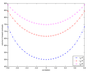
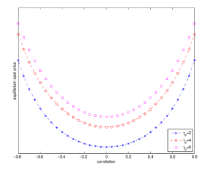
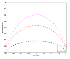
Figure 5.1: Equilibrium storage amount (top-left), volume in forward contracts (top-right), spot price (bottom-left) and forward premium (bottom-right) as a function of correlation for different values of the producers’ risk aversion $\gamma_{p}$.

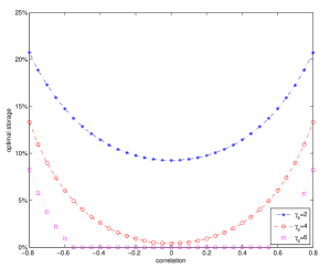
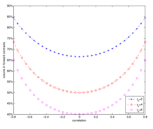
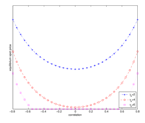
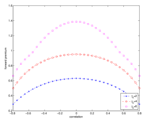
Figure 5.2: Equilibrium storage amount (top-left), volume in forward contracts (top-right), spot price (bottom-left) and forward premium (bottom-right) as a function of correlation for different values of the investors’ risk aversion $\gamma_{s}$.

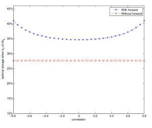
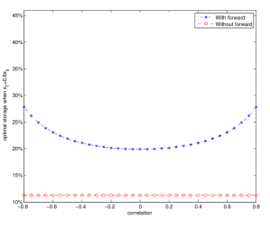
Figure 5.3: Equilibrium storage amount as a function of correlation for a market with and without forward contract. On the left $\pi_{T}=0.3\pi_{0}$ and on the right $\pi_{T}=0.6\pi_{0}$.

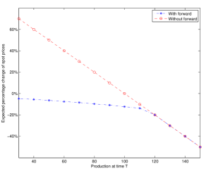
Figure 5.4: Expected percentage price changes $({\mathbb{E}}[\hat{P}_{T}]-\hat{P}_{0})/\hat{P}_{0}$ as a function of the production $\pi_{T}$ (given that $\pi_{0}=100$) with and without forward contract. On the left, the correlation $\rho=0.2$ and on the right $\rho=0.7$.

5.2 A jump-diffusion model

In the next example, the dynamics of the variates that determine the consumers’ demand and the financial market are driven by a Lévy jump-diffusion process, where the Brownian motion represents the ‘normal’ market behavior while the jumps appear simultaneously and represent some ‘shocks’, e.g. news announcements, that affect both the financial asset price and the demand for the commodity. More precisely, the dynamics of the processes $Y$ and $X$ are described by

$$Y_{t}=b_{1}t+\sigma_{1}W_{t}^{1}+\eta_{1}N_{t}\quad\text{ and }\quad X_{t}=b_{2}t+\sigma_{2}W_{t}^{2}+\eta_{2}N_{t},$$ (5.10)

where the drift term equals $b_{i}=\bar{b}_{i}-\lambda\eta_{i}$ with $\bar{b}_{i},\eta_{i}\in\mathbb{R}$ and $\sigma_{i}\in\mathbb{R}_{+}$, $i=1,2$. Furthermore, $W^{1},W^{2}$ are standard Brownian motions with correlation $\rho$, while $N$ is a univariate Poisson process with intensity $\lambda\in\mathbb{R}_{+}$. Hence, the constants $\eta_{1}$ and $\eta_{2}$ represent the effect of a jump in the financial market and the demand for the commodity, respectively.

Moreover, assuming $\bar{b}_{2}=0$ as in the previous example, the expectation of $X_{T}$ equals zero and using (2.8) we get that

$$\mathbb{E}[P_{T}]=\phi_{0}(\pi_{T})-\frac{\alpha(1-\varepsilon)}{m}\quad\text{ and }\quad\operatorname{\mathbb{V}ar}[P_{T}]=\frac{\sigma_{2}^{2}+\lambda\eta^{2}_{2}}{m^{2}}T.$$ (5.11)

Observe that the presence of jumps, either negative or positive, increases the variance of the spot price $P_{T}$ relative to the Brownian motion example. The next result provides an expression for the optimal inventory policy and the optimal investment in the forward contract.

Proposition 5.4.

Assuming the model dynamics provided by (5.10), the optimal strategy $\hat{\alpha},\hat{h}^{p}$ for the producers’ problem is provided by $\hat{\alpha}=(\alpha^{*}\vee 0)\wedge\pi_{0}$ and $\hat{h}^{p}=h^{p,*}(\hat{\alpha})$ where $(\alpha^{*},h^{p,*})$ solve the system of equations

$$\begin{cases}2\mathrm{d}_{1}\alpha+\mathrm{d}_{2}+\mathrm{d}_{3}h^{p}+\frac{\lambda\eta_{2}T(1-\varepsilon)}{m}\mathrm{e}^{-\gamma_{p}\eta_{2}\ell(\alpha,h^{p})}&=0,\\ \mathrm{d}_{3}\alpha+2\mathrm{d}_{4}h^{p}+\mathrm{d}_{5}+\frac{\lambda\eta_{2}T}{m}\mathrm{e}^{-\gamma_{p}\eta_{2}\ell(\alpha,h^{p})}&=0.\end{cases}$$ (5.12)

Here $\mathrm{d}_{1},\dots,\mathrm{d}_{5}$ are given by (A.1) by replacing $\operatorname{\mathbb{V}ar}[P_{T}]$ with $\frac{\sigma_{2}^{2}T}{m^{2}}$. The optimal investment for the investors’ problem $\hat{h}^{s}$ is provided by the solution to the equation

$$\frac{\partial}{\partial h^{s}}\left\{-\frac{T}{\gamma_{s}}\left[\widetilde{\kappa}{s}_{1}(\eta_{*})+\kappa_{2}\left(-\frac{\gamma_{s}h^{s}}{m}\right)\right]\right\}=F-\mathbb{E}[P_{T}],$$ (5.13)

where $\eta_{*}$ is given by (A.31).

The proof of the preceding Proposition is postponed for Appendix A.

Similarly to the previous example, the unique equilibrium forward price $\hat{F}$ is derived endogenously via the clearing condition (2.12), by noting again that $\hat{\alpha},\hat{h}^{p}$ and $\hat{h}^{s}$ depend on $\hat{F}$, and the equilibrium spot price of the commodity at the initial time is again given by (5.5). Therefore, in order to determine the equilibrium we need to solve equations (5.12) and (5.13). To this end, we have used numerical techniques, and have subsequently examined the impact of jumps on equilibrium quantities; see Figure 5.5 and the discussion in subsection 5.3.

Remark 5.5.

Using an independent Brownian motion instead of the Poisson process in (5.10), we can get the same first and second moments for $P_{T}$ as the ones in (5.11). This will also result in higher forward premia. However, jump processes are more appropriate models for the shocks that occur in random times and, in addition, jumps (in contrast to another Brownian motion) allow for asymmetries in the distributions, like fat tails and skewness. See also the discussion in the introduction of Section 4.

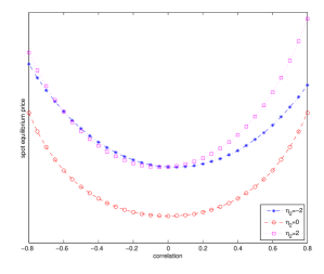
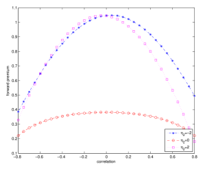
Figure 5.5: Equilibrium spot price (left) and forward premium (right) as a function of correlation for different values of the demand shock effect $\eta_{2}$ (in this example $\eta_{1}=0$).

5.3 Discussion of the results

Producers’ risk aversion and spot/forward prices

We can use the results above to create several figures that illustrate the effect of the model parameters on the equilibrium quantities. We first examine the producers’ side. The quantities that the producers have to consider are provided by $\underline{w}(\alpha,h^{p})$ in (2.1). We may split the terms into deterministic and stochastic ones. The deterministic part consists of the spot revenues from selling $\pi_{0}-\alpha$ units of the commodity at the spot price $P_{0}$, the expected future revenues from selling $\pi_{T}+\alpha(1-\varepsilon)$ units at the price ${\mathbb{E}}[P_{T}]$, and the expected payoff of the short position $h^{p}$ in forward contracts. The stochastic term stems from the randomness of the future price $P_{T}$ and equals $[\alpha(1-\varepsilon)+h^{p}+\pi_{T}]X/m$. One can readily see that the deterministic term is decreasing with respect to $\alpha$. However, the risk in the stochastic term is also reduced for decreasing storage amounts. Assuming that $\mathbb{E}[X]=0$, this risk is minimized when the quantity $\alpha(1-\varepsilon)+h^{p}+\pi_{T}$ vanishes, that is, when all the future sales are hedged. Hence, a large amount of the commodity in storage implies also a large position to be hedged and vice versa (all else equal).

Considering only the deterministic term, and assuming that $\mu$ is sufficiently large, producers have motive to store their production only if $\pi_{T}$ is relatively smaller than $\pi_{0}$ (recall the discussion in Remark 3.6). In any case, storing part of their production now increases the spot price of the commodity. In addition, because producers are risk averse, in order to hedge their future risk exposure, they are willing to share some of their future revenues by taking a short position in the forward contract. Naturally, the higher the risk aversion the larger the short position in the forward contract (see the top-right of Figure 5.1) and the higher the forward premium paid to the investors (see the bottom-right of Figure 5.1). Moreover, a larger position in forward contracts implies an increasing tendency for storage, thus higher risk aversion leads to increased storage amounts (see the top-left of Figure5.1). Summarizing, even when the production levels at time 0 and $T$ are close, producers with higher risk aversion tend to store more of their production when they can hedge the risk of future sales, a result which is consistent with the theory of storage, and this strategy increases the spot price of the commodity (see the bottom-left of Figure 5.1).

This result is further supported by the model without a forward contract in the market, see Remark 5.3. There, we observe that the only motive for the producers to store the commodity stems from the possible uneven productions (i.e. the difference between $\pi_{0}$ and $\pi_{T}$). This motive to store is increased when partial hedging is possible through the trading in forward contracts. In fact, as illustrated in Figure 5.3, the optimal storage is always higher in the model with forward contract, for every level of uneven productions, while for $\pi_{T}$ close to or higher than $\pi_{0}$, the optimal storage without forward contract is zero. Thus, spot prices in the model without forward contract are always lower compared to the model with forward. However, higher storage implies that the future expected spot price decreases (see for instance relation (5.2)), assuming that there is no rolling of the position in the forward contracts. Hence, while forward contracts tend to increase the spot commodity price, they also tend to decrease the future spot price. Therefore, the presence of forward contracts in the commodity market stabilizes prices when the production levels are uneven. This is apparent in Figure 5.4, where the expected price changes $({\mathbb{E}}[\hat{P}_{T}]-\hat{P}_{0})/\hat{P}_{0}$ are illustrated for different values of $\pi_{T}$. In this example, we note that when there is scarcity of the commodity at time $T$, forward contracts serve to stabilize commodity spot prices. On the contrary, when the production at initial time is lower than that at terminal time, then the expected price difference remains the same with and without the forward contract.

Let us also discuss the effect of jumps in the equilibrium quantities. Figure 5.5 illustrates the effect of a possible side shock in the consumers’ demand stemming from a jump. This jump not only increases the risk of the future price but it is also unhedgeable, since it is independent from the evolution of the stock market (we have assumed $\eta_{1}=0$). Therefore, the forward premium paid to the investors is higher, irrespective of the sign of the jump (see the right part of Figure 5.5). Moreover, when the future price is riskier, recalling the discussion above, we conclude that the more risk averse the producers are the more they increase the amount they store and hence they also increase the spot price of the commodity (see the left part of Figure 5.5). In addition, note that the sign of the jump makes little difference in the equilibrium quantities (if the expectation of the future demand shock is kept equal to zero).

The effect of the producers’ risk aversion on market equilibrium can be used to examine how the number of producers affects the equilibrium commodity prices. In the present framework of CARA preferences, the parameter $1/\gamma_{p}$ measures the producers’ aggregate risk tolerance. Therefore, if the number of producers increases, the parameter $\gamma_{p}$ decreases and the analysis above implies that equilibrium spot prices are lower, as expected.

Investors’ risk aversion and spot/forward prices

Let us now examine the investors’ side. When they become more risk averse, they are less willing to undertake the risk of a forward position. This is illustrated in Figure 5.2 (top-right), where the percentage $\hat{h}/(\pi_{T}+\hat{\alpha})$ (i.e. the percentage of forward contracts with respect to the total supply at time $T$) is plotted. Also, as the theory of normal backwardation states, more risk averse investors would require higher forward premium to enter into the forward contract. This premium is usually measured by the fraction $(\mathbb{E}[\hat{P}_{T}]-\hat{F})/\hat{F}$ which is plotted in Figure 5.2 (bottom-right). On the other hand, a higher forward premium implies that hedging is more expensive for the producers, hence they intend to supply more in the spot market and store less; note that the optimal storage amount even equals zero in some cases as the top-left of Figure 5.2 shows). Summarizing, when investors are more risk averse they invest less in forward contracts, which reduces the amount that producers can use for hedging; thus, producers offer more on the spot market, rendering equilibrium spot prices lower (see the bottom-left of Figure 5.2).

Turning our attention to the effect of the correlation between the consumers’ demand and the financial markets’ return, we note that the equilibrium quantities mainly depend on the square of $\rho$; this is basically because investors can go both long and short in the stock market. When $\rho^{2}$ increases, the effective risk aversion of the investors’, which is $\bar{\gamma}_{s}=\gamma_{s}(1-\rho^{2})$, decreases. Therefore, an increase of $\rho^{2}$ is eventually equivalent to a decrease of $\gamma_{s}$. This is expected because when the financial and the commodity markets are correlated, the investors can partially hedge the risk they undertake on a forward commodity contract by adjusting their investment strategy in the stock market accordingly. Hence, they become more risk tolerant. The dependence of the equilibrium quantities on the correlation coefficient $\rho$ is illustrated in Figure 5.2.

The effect of the investors’ risk aversion on market equilibrium can be used to examine how the number of investors affects the equilibrium commodity prices. In the present framework of CARA preferences, the parameter $1/\gamma_{s}$ measures the investors’ aggregate risk tolerance. Hence, if the number of investors increases, the parameter $\gamma_{s}$ considered in the above analysis decreases. As we have seen, the latter implies, among other things, higher equilibrium spot prices. This theoretical result is consistent with the observed comovement of the amounts invested in the commodity forward contracts and the commodity spot prices (see the related discussion in the introduction).

Convenience yield, correlation and uneven productions

As mentioned in the introduction, the convenience yield is a measure of the implicit benefit that inventory holders receive. Positivity of the convenience yield is consistent with the theory of storage. In our model, the convenience yield denoted by $y$ solves the equation

$$F=P_{0}\frac{1+R}{1-\varepsilon}-yP_{0},$$ (5.14)

see e.g. [1]. The relation of the yield with respect to the risk aversion coefficients of the producers and the investors is illustrated in Figure 5.6. As expected, $y$ is increasing with respect to both risk aversion coefficients (all else equal). The relation for the producers’ side follows readily from Figure 5.1, since higher producers’ risk aversion implies higher spot equilibrium price and higher forward premium (and also lower equilibrium forward price). Similarly, as the risk tolerance of the investors decreases, the cost of hedging increases, which makes producers sell more at the spot rather than storing and selling at a future date (see, in particular, the bottom-right of Figure 5.2).

The relation of the yield with respect to the correlation coefficient is more involved. When $\rho^{2}$ increases, there are two effects of opposite directions on the convenience yield. The first is negative and stems from the decrease of the investors’ effective risk aversion, while the second is positive and comes from the corresponding increase of the spot price (see the bottom-left of Figure 5.1). The final outcome depends on the level of the risk aversions and the difference of production levels (see Figures 5.6 and5.7). In particular, assuming that production levels are close to each other, when producers are sufficiently risk averse (tolerant), $y$ is decreasing (increasing) in $\rho^{2}$. Note also that the steep increase of the convenience yield when $\rho$ approaches zero (right graph on Figure 5.6) occurs when the storage is zero (compare with the top-left of Figure 5.2), since in this case only the negative effect of $\rho^{2}$ in the convenience yield occurs (when the storage is zero, the spot price does not increase).

On the other hand, the difference between the production levels $\pi_{0}$ and $\pi_{T}$ could change the monotonicity of the convenience yield with respect to the correlation coefficient. Indeed, when production at time $T$ is sufficiently larger than the initial production, storage is getting lower and hence the negative effect of $\rho$ in the convenience yield prevails. As the difference $\pi_{T}-\pi_{0}$ decreases, the positive effect that stems from the increased spot price is getting more influential, especially when producers are less risk averse (right of Figure 5.7).

Finally and as expected, for any correlation level, scarcity of commodity at initial time implies higher convenience yield (see both sides of Figure 5.7). In particular, when $\pi_{T}$ is sufficiently larger than $\pi_{0}$, the influence of the correlation $\rho$ on the convenience yield increases, a fact that reflects the producers’ benefit from satisfying their increased hedging through the forward contract (the latter is more intense when producers are more risk averse).

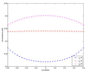
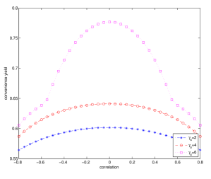
Figure 5.6: Equilibrium convenience yield as a function of correlation for different values of producers’ risk aversion $\gamma_{p}$ (left) and investors’ risk aversion $\gamma_{s}$ (right), when the production levels are equal ($\pi_{0}=\pi_{T}$).

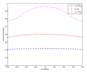
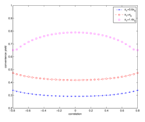
Figure 5.7: Equilibrium convenience yield as a function of correlation for different values of production levels, when producers are more risk averse (left) and less risk averse (right).

Remark 5.6.

In Acharya et al. [1], the authors present an extensive empirical analysis, based on an equilibrium model simpler than the one we have established and developed above. In Section 3 therein, data from spot and future markets of oil and gas is used for testing the predictions of the model. Our model offers a much richer set-up, not only regarding the families of probability distributions, but also because it includes in the analysis the relation of commodity and stock markets. One could apply similar methodology in order to test the predictions of our model, in particular the relation between the correlation of the stock market and the commodity demand with the forward premia, the volume in forward contracts and the optimal storage amount. We leave this interesting task as a subject for future research.

5.4 The effect of an existing hedge from a previous cycle

Aside from uneven production levels, another factor that decreases the producers’ tendency for storing is an already undertaken hedging position from a previous production and trading cycle. In this respect, we consider the situation where a forward contract with maturity $T$ was already issued during the previous cycle, and assume that producers have already taken a long position on it. We then examine how this existing hedge affects the spot and forward equilibrium quantities. More precisely, the total position of the producers’ takes the following form (compare to (2.1))

$$\underline{w}(\alpha,h^{p}) =P_{0}(\pi_{0}-\alpha)(1+R)+P_{T}(\pi_{T}+\alpha(1-\varepsilon))+h^{p}(P_{T}-F)+h^{\prime}(P_{T}-F^{\prime}),$$ (5.15)

where $h^{\prime}$ denotes the position in the forward contract with maturity at time $T$ that was bought with strike price $F^{\prime}$ at the previous cycle. The optimization problem for the producers has again the same form as in (2.3), and in particular for the model of subsection 5.1, it takes the form of the following quadratic programming problem:

$$\Pi^{p}=\underset{h^{p}\in\mathbb{R},\alpha\in[0,\pi_{0}]}{\max}\big{\{}\mathrm{d}_{1}\alpha^{2}+\mathrm{d}_{2}^{\prime}\alpha+\mathrm{d}_{3}\alpha h^{p}+\mathrm{d}_{4}(h^{p})^{2}+\mathrm{d}_{5}^{\prime}h^{p}+\mathrm{d}_{6}\big{\}},$$ (5.16)

where $\mathrm{d}_{1},\mathrm{d}_{3},\mathrm{d}_{4}$ remain the same and are provided by (A.1), while

$$\mathrm{d}_{2}^{\prime} =\frac{2(1+R)\pi_{0}-(1-\varepsilon)(2\pi_{T}+h^{\prime})-(R+\varepsilon)\mu}{m}-\gamma_{p}(1-\varepsilon)(\pi_{T}+h^{\prime})\operatorname{\mathbb{V}ar}[P_{T}]$$

$$\mathrm{d}_{5}^{\prime} =-\Big{(}F-\frac{\mu-\pi_{T}}{m}\Big{)}-\gamma_{p}(\pi_{T}+h^{\prime})\operatorname{\mathbb{V}ar}[P_{T}].$$

We observe that an existing long position in the forward contract, i.e. $h^{\prime}>0$, has the same impact as an increase of future production $\pi_{T}$. Therefore, as in Figures 5.3, positive $h^{\prime}$ implies less storage and hence lower spot equilibrium price. In addition, as in Figure 5.7, when producers have already hedged some of their risk, the convenience yield increases, a fact that reflects better inventory management. Similarly and as expected, a gradual hedging effectively serves to stabilize commodity prices (see Figure 5.4). This is because the tendency to increase spot prices by forward contracts is gradually applied to prices. Intuitively, when producers hedge the future price uncertainty by rolling their position in the forward contract, the effect on the spot prices is spread through time. Note, however, that an intimate analysis on the gradually optimal hedging requires a dynamic version of our equilibrium model, which is left open for future research.

Appendix A Proofs of Section 5

Proof A.1 (Proof of Proposition 5.1).

The model with dynamics (5.1) fits in the framework of Section 4 by considering a 2-dimensional Brownian motion $Z$ whose characteristic triplet has the form

$$b=\left(\begin{array}[]{c}b_{1}\\ 0\end{array}\right),\quad c=\left(\begin{array}[]{cc}\sigma_{1}^{2}&\rho\sigma_{1}\sigma_{2}\\ \rho\sigma_{1}\sigma_{2}&\sigma_{2}^{2}\end{array}\right)\quad\text{ and }\quad\nu\equiv 0,$$ (A.1)

where $b\in\mathbb{R}$, $\sigma_{1},\sigma_{2}\in\mathbb{R}_{+}$ and $\rho\in[-1,1]$, while the vectors $u_{1},u_{2}\in\mathbb{R}^{2}$ have the form

$$u_{1}=\left(\begin{array}[]{c}1\\ 0\\ \end{array}\right)\quad\text{ and }\quad u_{2}=\left(\begin{array}[]{c}0\\ 1\\ \end{array}\right).$$ (A.2)

The cumulant generating functions of $Y_{1}=\left\langle u_{1},Z_{1}\right\rangle$ and $X_{1}=\left\langle u_{2},Z_{1}\right\rangle$ are given by

$$\kappa_{1}(v)=vb_{1}+\frac{v^{2}\sigma_{1}^{2}}{2}\quad\text{ and }\quad\kappa_{2}(v)=\frac{v^{2}\sigma_{2}^{2}}{2}.$$ (A.3)

The set $\mathcal{U}_{Z}$ equals $\mathbb{R}^{2}$, thus Assumption $(\mathbb{EM})$ and (3.27) are trivially satisfied, while the same is true for Assumption $(\mathbb{FE})$ since $\nu\equiv 0$. Assumption $(\mathbb{COE})$ is also satisfied due to $\kappa_{2}$ being quadratic in $u$, while Assumption $(\mathbb{NA}^{\prime})$ is fulfilled since we can construct a martingale measure under which $Z$ remains a Brownian motion.

Starting with the producers’ side, the optimal hedging and storage positions are determined by Proposition 3.3 and (4.10), leading to the following quadratic programming problem:

$$\Pi^{p}=\underset{h^{p}\in\mathbb{R},\alpha\in[0,\pi_{0}]}{\max}\big{\{}\mathrm{d}_{1}\alpha^{2}+\mathrm{d}_{2}\alpha+\mathrm{d}_{3}\alpha h^{p}+\mathrm{d}_{4}(h^{p})^{2}+\mathrm{d}_{5}h^{p}+\mathrm{d}_{6}\big{\}},$$ (A.4)

where

$$\mathrm{d}_{1} =-\left(\frac{1+R+(1-\varepsilon)^{2}}{m}+\frac{\gamma_{p}(1-\varepsilon)^{2}}{2}\operatorname{\mathbb{V}ar}[P_{T}]\right)$$

$$\mathrm{d}_{2} =\frac{2(1+R)\pi_{0}-2(1-\varepsilon)\pi_{T}-(R+\varepsilon)\mu}{m}-\gamma_{p}(1-\varepsilon)\pi_{T}\operatorname{\mathbb{V}ar}[P_{T}]$$

$$\mathrm{d}_{3} =-\frac{1-\varepsilon}{m}-\gamma_{p}(1-\varepsilon)\operatorname{\mathbb{V}ar}[P_{T}]$$ (A.5)

$$\mathrm{d}_{4} =-\frac{\gamma_{p}}{2}\operatorname{\mathbb{V}ar}[P_{T}]$$

$$\mathrm{d}_{5} =-\Big{(}F-\frac{\mu-\pi_{T}}{m}\Big{)}-\gamma_{p}\pi_{T}\operatorname{\mathbb{V}ar}[P_{T}].$$

The first order conditions yield the following solutions

$$h^{p,*}=-\frac{\alpha\mathrm{d}_{3}+\mathrm{d}_{5}}{2\mathrm{d}_{4}}\quad\text{ and }\quad\alpha^{*}=\frac{\mathrm{d}_{3}\mathrm{d}_{5}-2\mathrm{d}_{2}\mathrm{d}_{4}}{4\mathrm{d}_{1}\mathrm{d}_{4}-\mathrm{d}_{3}^{2}}.$$ (A.6)

Therefore, the optimal strategy $(\hat{\alpha},\hat{h}^{p})\in[0,\pi_{0}]\times\mathbb{R}$ for the producers’ problem is provided by

$$\hat{\alpha}=(\alpha^{*}\vee 0)\wedge\pi_{0}\quad\text{ and }\quad\hat{h}^{p}=-\frac{\hat{\alpha}\mathrm{d}_{3}+\mathrm{d}_{5}}{2\mathrm{d}_{4}}.$$ (A.7)

Next, we turn our attention to the investors’ problem and follow the strategy outlined in subsection 4.2. The cumulant generating function of $Z$ under $\mathbb{P}{s}$ is provided by

$$\kappa{s}(v)=\left\langle v-\xi,b\right\rangle+\frac{\left\langle v-\xi,c(v-\xi)\right\rangle}{2},$$ (A.8)

where $\xi=-\frac{\gamma_{s}h^{s}}{m}u_{2}$. In particular, the characteristics of $Y$ under $\mathbb{P}{s}$ are

$$b_{1}{s}=b_{1}-\rho\sigma_{1}\sigma_{2}\frac{\gamma_{s}h^{s}}{m}\quad\text{ and }\quad c_{1}{s}=\sigma_{1}^{2},$$ (A.9)

thus the characteristics of the exponential transform $\widetilde{Y}$ under $\mathbb{P}{s}$ are

$$\widetilde{b}_{1}{s}=b_{1}-\rho\sigma_{1}\sigma_{2}\frac{\gamma_{s}h^{s}}{m}+\frac{\sigma_{1}^{2}}{2}\quad\text{ and }\quad\widetilde{c}_{1}{s}=\sigma_{1}^{2}.$$ (A.10)

The cumulant generating function of $\widetilde{Y}$ simply has the form

$$\widetilde{\kappa}_{1}{s}(v)=v\Big{(}b_{1}-\rho\sigma_{1}\sigma_{2}\frac{\gamma_{s}h^{s}}{m}+\frac{\sigma_{1}^{2}}{2}\Big{)}+\frac{v^{2}\sigma_{1}^{2}}{2},$$ (A.11)

and its derivative obviously equals

$$\frac{\partial}{\partial v}\widetilde{\kappa}_{1}{s}(v)=b_{1}-\rho\sigma_{1}\sigma_{2}\frac{\gamma_{s}h^{s}}{m}+\frac{\sigma_{1}^{2}}{2}+v\sigma_{1}^{2}.$$ (A.12)

Therefore, the solution to equation (4.20) is

$$\eta^{*}=\rho\frac{\sigma_{2}}{\sigma_{1}}\frac{\gamma_{s}h^{s}}{m}-\frac{b_{1}}{\sigma_{1}^{2}}-\frac{1}{2},$$ (A.13)

and the minimal entropy equals

$$\mathcal{H}(\mathbb{P}_{*}|\mathbb{P}{s})=\frac{T}{2}(\eta^{*}\sigma_{1})^{2}=\frac{T}{2}\Big{(}\lambda-\rho\sigma_{2}\frac{\gamma_{s}h^{s}}{m}\Big{)}^{2}.$$ (A.14)

Here $\lambda$ denotes the ‘market price of risk’ for the asset $S$, i.e. $\lambda=\frac{\mu_{1}-r}{\sigma_{1}}$, with $\mu_{1}$ being the expected rate of return of $S$ and $r$ the continuously compounded interest rate, while we have also used that $b_{1}=\mu_{1}-r-\sigma_{1}^{2}/2$.

The investors’ optimal position in the forward contract is determined by (4.28), leading to the following quadratic optimization problem:

$$\Pi^{s}=\max_{h^{s}\in\mathbb{R}}\big{\{}\mathrm{d}_{7}(h^{s})^{2}+\mathrm{d}_{8}h^{s}+\mathrm{d}_{9}\big{\}},$$ (A.15)

where

$$\mathrm{d}_{7} =-\frac{\gamma_{s}}{2}(1-\rho^{2})\operatorname{\mathbb{V}ar}[P_{T}]$$ (A.16)

$$\mathrm{d}_{8} =\mathbb{E}[P_{T}]-F-\lambda\rho\sqrt{T}\sqrt{\operatorname{\mathbb{V}ar}[P_{T}]}.$$ (A.17)

Applying the first order conditions once again, we arrive at the optimal position for the investors

$$\hat{h}^{s}=\frac{\mathbb{E}[P_{T}]-F}{\bar{\gamma}_{s}\operatorname{\mathbb{V}ar}[P_{T}]}-\frac{\lambda\rho\sqrt{T}}{\bar{\gamma}_{s}\sqrt{\operatorname{\mathbb{V}ar}[P_{T}]}},$$ (A.18)

where $\bar{\gamma}_{s}=\gamma_{s}(1-\rho^{2})$.

Proof A.2 (Proof of Proposition 5.4).

The model with dynamics (5.10) fits in the framework of Section 4 by considering a 2-dimensional Lévy process $Z$ whose characteristic triplet has the form

$$b=\left(\begin{array}[]{c}b_{1}\\ b_{2}\end{array}\right),\,\,\,\,c=\left(\begin{array}[]{cc}\sigma_{1}^{2}&\rho\sigma_{1}\sigma_{2}\\ \rho\sigma_{1}\sigma_{2}&\sigma_{2}^{2}\end{array}\right)\,\,\,\,\text{ and }\,\,\,\,\nu(\mathrm{d}x_{1},\mathrm{d}x_{2})=\lambda 1_{\{\eta_{1},\eta_{2}\}}(\mathrm{d}x_{1},\mathrm{d}x_{2}),$$ (A.19)

while the vectors $u_{1},u_{2}\in\mathbb{R}^{2}$ are provided by (A.2). The cumulant generating function of $Y_{1}=\left\langle u_{1},Z_{1}\right\rangle$ and $X_{1}=\left\langle u_{2},Z_{1}\right\rangle$ is given by

$$\kappa_{i}(v) =vb_{i}+\frac{v^{2}\sigma_{i}^{2}}{2}+\lambda\left(\mathrm{e}^{v\eta_{i}}-1\right)\quad i=1,2.$$ (A.20)

The set $\mathcal{U}_{Z}$ equals $\mathbb{R}^{2}$, thus Assumption $(\mathbb{EM})$ and (3.27) are trivially satisfied, while the same is true for Assumption $(\mathbb{FE})$. Assumption $(\mathbb{COE})$ is also satisfied due to $\kappa_{2}$ being quadratic in $v$, while Assumption $(\mathbb{NA}^{\prime})$ is satisfied since we can construct a martingale measure under which $X$ has finite first moment.

Starting with the producers side, the optimal hedging and storage positions are provided by Proposition 3.3 and (4.10), leading to the following optimization problem:

$$\Pi^{p}=\underset{h^{p}\in\mathbb{R},\alpha\in[0,\pi_{0}]}{\max}f(\alpha,h^{p})$$ (A.21)

where

$$f(\alpha,h^{p}):=\mathrm{d}_{1}\alpha^{2}+\mathrm{d}_{2}\alpha+\mathrm{d}_{3}\alpha h^{p}+\mathrm{d}_{4}(h^{p})^{2}+\mathrm{d}_{5}h^{p}+\mathrm{d}_{6}+j(\alpha,h^{p}),$$ (A.22)

with

$$j(\alpha,h^{p}):=-\lambda\left(\mathrm{e}^{-\gamma_{p}\eta_{2}\ell(\alpha,h^{p})}-1\right)\frac{T}{\gamma_{p}}.$$ (A.23)

The coefficients $\mathrm{d}_{1},\dots,\mathrm{d}_{5}$ are provided by (A.1) by replacing $\operatorname{\mathbb{V}ar}[P_{T}]$ with $\frac{\sigma_{2}^{2}T}{m}$. The first order optimality conditions lead to the system of non-linear equations (5.12), i.e.

$$\begin{cases}\frac{\partial}{\partial\alpha}f(\alpha,h^{p})&=2\mathrm{d}_{1}\alpha+\mathrm{d}_{2}+\mathrm{d}_{3}h^{p}+\frac{\lambda\eta_{2}T(1-\varepsilon)}{m}\mathrm{e}^{-\gamma_{p}\eta_{2}\ell(\alpha,h^{p})}=0,\\ \frac{\partial}{\partial h^{p}}f(\alpha,h^{p})&=\mathrm{d}_{3}\alpha+2\mathrm{d}_{4}h^{p}+\mathrm{d}_{5}+\frac{\lambda\eta_{2}T}{m}\mathrm{e}^{-\gamma_{p}\eta_{2}\ell(\alpha,h^{p})}=0,\end{cases}$$ (A.24)

and its solution is denoted by $(\alpha^{*},h^{p,*})$, where the relation of $\alpha^{*}$ and $h^{p,*}$ is given by the following linear equation

$$\alpha^{*}=\frac{2(1-\varepsilon)\mathrm{d}_{4}-\mathrm{d}_{3}}{2\mathrm{d}_{1}-(1-\varepsilon)\mathrm{d}_{3}}h^{p,*}+\frac{(1-\varepsilon)\mathrm{d}_{5}-\mathrm{d}_{2}}{2\mathrm{d}_{1}-(1-\varepsilon)\mathrm{d}_{3}}.$$

Therefore, the optimal strategy $(\hat{\alpha},\hat{h}^{p})\in[0,\pi_{0}]\times\mathbb{R}$ for the producers problem is provided by

$$\hat{\alpha}=(\alpha^{*}\vee 0)\wedge\pi_{0}\quad\text{ and }\quad\hat{h}^{p}=h^{p,*}(\hat{\alpha}).$$ (A.25)

Next, we turn our attention to the investors problem and follow again the strategy of subsection 4.2. The characteristics of $Y$ under $\mathbb{P}{s}$ are provided by Lemma 4.2, thus using (A.19) we get that

$$b_{1}{s} =b_{1}-\rho\sigma_{1}\sigma_{2}\zeta+\lambda\eta_{1}(\mathrm{e}^{-\eta_{2}\zeta}-1)$$

$$c_{1}{s} =\sigma_{1}^{2}$$ (A.26)

$$1_{E}(y)*\nu_{1}{s} =1_{E}(\left\langle u_{1},x\right\rangle)\mathrm{e}^{\left\langle\xi,x\right\rangle}*\nu,$$

where $\zeta:=\frac{\gamma_{s}h^{s}}{m}$, $E\in\mathcal{B}(\mathbb{R})$ and “$*$” denotes integration. Therefore, the cumulant generating function of $Y$ under $\mathbb{P}{s}$ takes the form

$$\kappa_{1}{s}(v)=vb_{1}{s}+\frac{v^{2}\sigma_{1}^{2}}{2}+\lambda(\mathrm{e}^{v\eta_{1}}-1)\mathrm{e}^{-\zeta\eta_{2}}.$$ (A.27)

Moreover, the characteristics of the exponential transform $\widetilde{Y}$ of $Y$ are provided by (4.2), thus we obtain that

$$\widetilde{b}{s}_{1} =\kappa_{1}{s}(1)$$

$$\widetilde{c}_{1}{s} =\sigma_{1}^{2}$$ (A.28)

$$1_{E}(z)*\widetilde{\nu}_{1}{s} =1_{E}(\mathrm{e}^{y}-1)*\nu_{1}{s}.$$

Hence, the cumulant generating function of $\widetilde{Y}$ under $\mathbb{P}{s}$ equals

$$\widetilde{\kappa}{s}_{1}(v) =v\widetilde{b}{s}_{1}+\frac{v^{2}\sigma_{1}^{2}}{2}+\lambda\mathrm{e}^{-\eta_{2}\zeta}\left(\mathrm{e}^{v(\mathrm{e}^{\eta_{1}}-1)}-1\right)$$ (A.29)

and its derivative with respect to $v$ equals

$$\frac{\partial}{\partial v}\widetilde{\kappa}{s}_{1}(v) =\widetilde{b}{s}_{1}+v\sigma_{1}^{2}+\lambda\mathrm{e}^{-\eta_{2}\zeta}\mathrm{e}^{v(\mathrm{e}^{\eta_{1}}-1)}(\mathrm{e}^{\eta_{1}}-1).$$ (A.30)

The minimal entropy martingale measure is determined by the solution $\eta_{*}$ to the non-linear equation

$$\widetilde{b}{s}_{1}+\eta_{*}\sigma_{1}^{2}+\lambda\mathrm{e}^{-\eta_{2}\zeta}\mathrm{e}^{\eta_{*}(\mathrm{e}^{\eta_{1}}-1)}(\mathrm{e}^{\eta_{1}}-1)=0,$$ (A.31)

and then the minimal entropy equals

$$\mathcal{H}(\mathbb{P}_{*}|\mathbb{P}{s})=-\frac{T}{\gamma_{s}}\widetilde{\kappa}{s}_{1}(\eta_{*}).$$ (A.32)

Now, putting the pieces together, the investors optimization problem takes the form

$$\Pi^{s}=\max_{h^{s}}g(h^{s})$$ (A.33)

where

$$g(h^{s}):=-\frac{T}{\gamma_{s}}\left\{\widetilde{\kappa}{s}_{1}(\eta_{*})+\kappa_{2}\left(-\frac{\gamma_{s}h^{s}}{m}\right)\right\}+h^{s}\big{(}{\mathbb{E}}[P_{T}]-F\big{)},$$ (A.34)

and the maximizer is determined by the first order conditions, leading to (5.13).

References

- Acharya et al. [2013] V.V. Acharya, A.L. Lochstoer, and T. Ramadorai. Limits to arbitrage and hedging: Evidence from commodity markets. Journal of Financial Economics, 109:441–465, 2013.
- Anderson and Danthine [1980] R.W. Anderson and J.-P. Danthine. Hedging and joint production: Theory and illustrations. Journal of Finance, 35:487–498, 1980.
- Anderson and Danthine [1983] R.W. Anderson and J.-P. Danthine. Hedger diversity in futures markets. Economic Journal, 93:370–389, 1983.
- Anthropelos and Žitković [2010] M. Anthropelos and G. Žitković. On agent’s agreement and partial-equilibrium pricing in incomplete markets. Mathematical Finance, 20:411–446, 2010.
- Applebaum [2009] D. Applebaum. Lévy Processes and Stochastic Calculus. Cambridge University Press, 2nd edition, 2009.
- Baker [2014] S. D. Baker. The financialization of storable commodities. Preprint, ssrn:2348333, 2014.
- Barrieu and El Karoui [2009] P. Barrieu and N. El Karoui. Pricing, hedging and designing derivatives with risk measures. In R. Carmona, editor, Indifference Pricing: Theory and Applications, pages 77–145. Princeton University Press, 2009.
- Basak and Pavlova [2016] S. Basak and A. Pavlova. A model of financialization of commodities. Journal of Finance, 2016. (forthcoming).
- Brennan [1958] M. Brennan. The supply of storage. American Economic Review, 48:50–72, 1958.
- Buyuksahin and Robe [2014] B. Buyuksahin and M.A. Robe. Speculators, commodities and cross-market linkages. Journal of International Money and Finance, 42:38–70, 2014.
- Caldentey and Haugh [2006] R. Caldentey and M. Haugh. Optimal control and hedging of operations in the presence of financial markets. Mathematics of Operations Research, 31:285–304, 2006.
- Carr et al. [2002] P. Carr, H. Geman, D. B. Madan, and M. Yor. The fine structure of asset returns: An empirical investigation. Journal of Business, 75:305–332, 2002.
- Casassus et al. [2008] J. Casassus, P. Collin-Dufresne, and B. Routledge. Equilibrium commodity prices with irreversible investment and non-linear technologies. NBER Working Paper No. 11864, 2008.
- Cheridito [2013] P. Cheridito. Convex analysis. Lecture notes, Princeton University, 2013.
- Cheridito et al. [2016] P. Cheridito, U. Horst, M. Kupper, and T. Pirvu. Equilibrium pricing in incomplete markets under translation invariant preferences. Mathematics of Operations Research, 41:174–195, 2016.
- Cherny and Shiryaev [2002] A. S. Cherny and A. N. Shiryaev. Change of time and measure for Lévy processes. Lecture Notes, University of Aarhus, 2002.
- Com [2008] Staff Report on Commodity Swap Dealers and Index Traders with Commission Recommendations. Commodity Futures Trading Commission, 2008.
- Cont and Tankov [2004] R. Cont and P. Tankov. Financial Modelling with Jump Processes. Chapman and Hall/CRC Press, 2004.
- Delbaen et al. [2002] F. Delbaen, P. Grandits, T. Rheinländer, D. Samperi, M. Schweizer, and C. Stricker. Exponential hedging and entropic penalties. Mathematical Finance, 12:99–123, 2002.
- Eberlein [2001] E. Eberlein. Application of generalized hyperbolic Lévy motions to finance. In O. E. Barndorff-Nielsen, T. Mikosch, and S. I. Resnick, editors, Lévy Processes: Theory and Applications, pages 319–336. Birkhäuser, 2001.
- Eberlein and Glau [2014] E. Eberlein and K. Glau. Variational solutions of the pricing PIDEs for European options in Lévy models. Applied Mathematical Finance, 21:417–450, 2014.
- Eberlein and Jacod [1997] E. Eberlein and J. Jacod. On the range of options prices. Finance and Stochastics, 1:131–140, 1997.
- Eberlein et al. [2009] E. Eberlein, A. Papapantoleon, and A. N. Shiryaev. Esscher transform and the duality principle for multidimensional semimartingales. Annals of Applied Probability, 19:1944–1971, 2009.
- Ekeland et al. [2014] I. Ekeland, D. Lautier, and B. Villeneuve. Speculation in commodity futures markets: A simple equilibrium model. Working paper, Université Paris-Dauphine, 2014.
- Filipović and Kupper [2008] D. Filipović and M. Kupper. Equilibrium prices for monetary utility functions. International Journal of Theoretical and Applied Finance, 11:325–343, 2008.
- Föllmer and Schied [2004] H. Föllmer and A. Schied. Stochastic Finance. de Gruyter, 2nd edition, 2004.
- Fujiwara [2004] T. Fujiwara. From the minimal entropy martingale measures to the optimal strategies for the exponential utility maximization: the case of geometric Lévy processes. Asia-Pacific Financial Markets, 11:367–391, 2004.
- Fujiwara and Miyahara [2003] T. Fujiwara and Y. Miyahara. The minimal entropy martingale measures for geometric Lévy processes. Finance and Stochastics, 7:509–531, 2003.
- Gorton and Rouwenhorst [2006] G. B. Gorton and K. G. Rouwenhorst. Facts and Fantasies about Commodity Futures. Financial Analysts Journal, 62:47–68, 2006.
- Gorton et al. [2012] G. B. Gorton, F. Hayashi, and K. G. Rouwenhorst. The fundamentals of commodity futures returns. Review of Finance, 17:35–105, 2012.
- Hamilton [2009] J. D. Hamilton. Causes and consequences of the oil shock of 2007–08. Brookings Papers on Economic Activity, 1:215–261, 2009.
- Hamilton and Wu [2015] J. D. Hamilton and C. Wu. Effects of index-fund investing on commodity futures prices. International Economic Review, 56:187–205, 2015.
- Henderson et al. [2015] B.J. Henderson, N.D. Pearson, and L. Wang. New evidence on the financialization of commodity markets. Review of Financial Studies, 28:1285–1311, 2015.
- Hicks [1939] J.R. Hicks. Value and Capital. Oxford University Press, 1939.
- Hirshleifer [1988] D. Hirshleifer. Residual risk, trading costs, and commodity futures risk premiums. Review of Financial Studies, 1:173–193, 1988.
- Hirshleifer [1989] D. Hirshleifer. Futures trading, storage and the division of risk: A multiperiod analysis. Economic Journal, 99:700–719, 1989.
- Horst and Müller [2007] U. Horst and M. Müller. On the spanning property of risk bonds priced by equilibrium. Mathematics of Operations Research, 32:784–807, 2007.
- Hubalek and Sgarra [2006] F. Hubalek and C. Sgarra. Esscher transforms and the minimal entropy martingale measure for exponential Lévy models. Quantitative Finance, 6:125–145, 2006.
- Juvenal and Petrella [2012] L. Juvenal and I. Petrella. Speculation in oil market. Working paper, Federal Reserve Bank of Saint Louis, 2012.
- Kaldor [1939] N. Kaldor. Speculation and economic stability. Review of Economic Studies, 7:1–27, 1939.
- Kallsen and Shiryaev [2002] J. Kallsen and A. N. Shiryaev. The cumulant process and Esscher’s change of measure. Finance and Stochastics, 6:397–428, 2002.
- Karatzas et al. [1990] I. Karatzas, J.P. Lehoczky, and S.E. Shreve. Existence and uniqueness of multi-agent equilibrium in a stochastic, dynamic consumption/investment model. Mathematics of Operations Research, 15:80–128, 1990.
- Keynes [1930] J.M. Keynes. A Treatise on Money, Vol. 2. Macmillan, London, 1930.
- Kilian and Murphy [2014] L. Kilian and D.P. Murphy. The role of inventories and speculative trading in the global market for crude oil. Journal of Applied Econometrics, 29:454–478, 2014.
- Knittel and Pindyck [2013] C. Knittel and R. Pindyck. The simple economics of commodity price speculation. NBER Working Paper No. 18951, 2013.
- Kyprianou [2006] A. E. Kyprianou. Introductory Lectures on Fluctuations of Lévy Processes with Applications. Springer, 2006.
- Laeven and Stadje [2014] R.J.A. Laeven and M. Stadje. Robust portfolio choice and indifference valuation. Mathematics of Operations Research, 39:1109–1141, 2014.
- Leclercq and Praz [2014] E. Leclercq and R. Praz. Equilibirum commodity trading. Preprint, ssrn:2464400, 2014.
- Pirrong [2011] C. Pirrong. Commodity Price Dynamics: A Structural Approach. Cambridge University Press, 2011.
- Rockafellar [1997] R. T. Rockafellar. Convex Analysis. Princeton University Press, 1997.
- Routledge et al. [2000] B.R. Routledge, D.J. Seppi, and C.S. Spatt. Equilibrium forward curves for commodities. Journal of Finance, 60:1297–1338, 2000.
- Rouwenhorst and Tang [2012] K.G. Rouwenhorst and K. Tang. Commodity Investing. Annual Review of Financial Economics, 4:447–467, 2012.
- Sato [1999] K. Sato. Lévy Processes and Infinitely Divisible Distributions. Cambridge University Press, 1999.
- Schoutens [2003] W. Schoutens. Lévy Processes in Finance: Pricing Financial Derivatives. Wiley, 2003.
- Shiryaev [1999] A. N. Shiryaev. Essentials of Stochastic Finance: Facts, Models, Theory. World Scientific, 1999.
- Singleton and Thorp [2013] A. Singleton and S. Thorp. Financialization, crisis and commodity correlation dynamics. Journal of International Financial Markets, Institutions and Money, 24:42–65, 2013.
- Singleton [2014] K. J. Singleton. Investor flows and the 2008 boom/bust in oil prices. Management Science, 60:300–318, 2014.
- Stoll [1979] H. Stoll. Commodity futures and spot price determination and hedging in capital market equilibrium. Journal of Financial and Quantitative Analysis, 14:873–894, 1979.
- Stoll and Whaley [2010] H. Stoll and R. Whaley. Commodity index investing and commodity futures prices. Journal of Applied Finance, 20:7–46, 2010.
- Tang and Xiong [2012] K. Tang and W. Xiong. Index investing and the financialization of commodities. Financial Analysts Journal, 68(6):54–74, 2012.
- Wilson [1968] R. Wilson. The theory of syndicates. Econometrica, 36:119–132, 1968.
- Working [1949] H. Working. The theory of the price of storage. American Economic Review, 39:1254–1262, 1949.