Efficient model-based reinforcement learning for approximate online optimal control

Abstract

In this paper the infinite horizon optimal regulation problem is solved online for a deterministic control-affine nonlinear dynamical system using the state following (StaF) kernel method to approximate the value function. Unlike traditional methods that aim to approximate a function over a large compact set, the StaF kernel method aims to approximate a function in a small neighborhood of a state that travels within a compact set. Simulation results demonstrate that stability and approximate optimality of the control system can be achieved with significantly fewer basis functions than may be required for global approximation methods.

I Introduction

Reinforcement learning (RL) has become a popular tool for determining online solutions of optimal control problems for systems with finite state and action spaces[1, 2, 3]. Due to technical challenges, implementation of RL in systems with continuous state and action spaces has remained an open problem. In recent years, adaptive dynamic programming (ADP) has been successfully used to implement RL in deterministic autonomous control-affine systems to solve optimal control problems via value function approximation [4, 5, 6, 7, 8, 3, 9, 10, 11, 12, 13]. ADP techniques employ parametric function approximation (typically by employing neural networks (NNs)) to approximate the value function. Implementation of function approximation in ADP is challenging because the controller is void of pre-designed stabilizing feedback and is completely defined by the estimated parameters. Hence, the error between the optimal and the estimated value function is required to decay to a sufficiently small bound sufficiently fast to establish closed-loop stability. The size of the error bound is determined by the selected basis functions, and the convergence rate is determined by richness of the data used for learning.

Sufficiently accurate approximation of the value function over a sufficiently large neighborhood often requires a large number of basis functions, and hence, introduces a large number of unknown parameters. One way to achieve accurate function approximation with fewer unknown parameters is to use some knowledge about the system to determine the basis functions. However, for general nonlinear systems, prior knowledge of the features of the optimal value function is generally not available; hence, a large number of generic basis functions is often the only feasible option.

Sufficiently fast approximation of the value function over a sufficiently large neighborhood requires sufficiently rich data to be available for learning. In traditional ADP methods such as [14, 9, 11], richness of data manifests itself as the amount of excitation in the system. In experience replay-based techniques such as [15, 16, 17, 18], richness of data is quantified by eigenvalues of the recorded history stack. In model-based RL techniques such as [19, 20, 21], richness of data corresponds to the eigenvalues of a learning matrix. As the dimension of the system and the number of basis functions increases, the required richness of data increases. In traditional ADP methods, the demand for richer data causes the designer to design increasingly aggressive excitation signals, thereby causing undesirable oscillations. Hence, implementation of traditional ADP techniques such as [4, 5, 6, 7, 8, 3, 14, 9, 10, 11, 12, 13] in high dimensional systems are seldom found in the literature. In experience replay-based ADP methods and in model-based RL, the demand for richer data causes the required amount of data stored in the history stack, and the number of points selected to construct the learning matrix, respectively, to grow exponentially with the dimension of the system. Hence, implementation of data-driven ADP techniques such as [19, 20, 18, 22, 23, 21] are scarcely found in the literature.

The contribution of this paper is the development of a novel model-based RL technique to achieve sufficient excitation without causing undesirable oscillations and expenditure of control effort like traditional ADP techniques and at a lower computational cost than state-of-the-art data-driven ADP techniques. Motivated by the fact that the computational effort required to implement ADP and the data-richness required to achieve convergence decrease with decreasing number of basis functions, this paper focuses on reduction of the number of basis functions used for value function approximation. A key contribution of this paper is the observation that online implementation of an ADP-based approximate optimal controller does not require an estimate of the optimal value function over the entire domain of operation of the system. Instead, only an estimate of the slope of the value function evaluated at the current state is required for feedback. Hence, estimation of the value function over a small neighborhood of the current state should be sufficient to implement an ADP-based approximate optimal controller. Furthermore, it is reasonable to postulate that approximation of the value function over a smaller local domain would require fewer basis functions as opposed to approximation over the entire domain of operation.

In this paper, reduction in the number of basis functions required for value function approximation is achieved via selection of basis functions that travel with the system state (referred to as state-following (StaF) kernels) to achieve accurate approximation of the value function over a small neighborhood of the state. The use of StaF kernel introduces a technical challenge owing to the fact that the ideal values of the unknown parameters corresponding to the StaF kernels are functions of the system state. The Lyapunov-based stability analysis presented in Section IV explicitly incorporates this functional relationship using the result that the ideal weights are continuously differentiable functions of the system state.

Sufficient exploration without the addition of an aggressive excitation signal is achieved via model-based RL based on BE extrapolation [19, 20]. The computational load associated with BE extrapolation is reduced via the selection of a single time-varying extrapolation function instead of a large number of autonomous extrapolation functions used in [19, 20]. Stability and convergence to optimality are obtained under a PE condition on the extrapolated regressor. Intuitively, selection of a single time-varying BE extrapolation function results in virtual excitation. That is, instead of using input-output data from a persistently excited system, the dynamic model is used to simulate persistent excitation to facilitate parameter convergence. Simulation results are included to demonstrate the effectiveness of the developed technique.

II StaF Kernel Functions

The objective in StaF-based function approximation is to maintain good approximation of the target function in a small region of interest in the neighborhood of a point of interest $x\in\mathbb{R}^{n}$. In state-of-the-art online approximate control, the optimal value function is approximated using a linear-in-the-parameters approximation scheme, and the approximate control law drives the system along the steepest negative gradient of the approximated value function. To compute the controller at the current state, only the gradient of the value function evaluated at the current state is required. Hence, in this application, the target function is the optimal value function, and the point of interest is the system state.

Since the system state evolves through the state-space with time, the region of interest for function approximation also evolves through the state-space. The StaF technique aims to maintain a uniform approximation of the value function over a small region around the current system state so that the gradient of the value function at the current state, and hence, the optimal controller at the current state, can be approximated.

To facilitate the theoretical development, this section summarizes key results from [24], where the theory of reproducing kernel Hilbert spaces (RKHSs) is used to establish continuous differentiability of the ideal weights with respect to the system state, and the postulate that approximation of the value function over a small neighborhood of the current state would require fewer basis functions is stated and proved.

To facilitate the discussion, let $H$ be a universal RKHS over a compact set $\chi\subset\mathbb{R}^{n}$ with a continuously differentiable positive definite kernel $k:\chi\times\chi\to\mathbb{R}$. Let $\overline{V}^{*}:\chi\to\mathbb{R}$ be a function such that $\overline{V}^{*}\in H$ . Let $c\triangleq\left[c_{1},c_{2},\cdots c_{L}\right]^{T}\in\chi^{L}$ be a set of distinct centers, and let $\sigma:\chi\times\chi^{L}\to\mathbb{R}^{L}$ be defined as $\sigma\left(x,c\right)=\left[k\left(x,c_{1}\right),\cdots,k\left(x,c_{L}\right)\right]^{T}$. Then, there exists a unique set of weights $W_{H}$ such that

$$W_{H}\left(c\right)=\arg\min_{a\in\mathbb{R}^{L}}\left\|a^{T}\sigma(\cdot,c)-\overline{V}^{*}\right\|_{H},$$

where $\left\|\cdot\right\|_{H}$ denotes the Hilbert space norm.

In the StaF approach, the centers are selected to follow the current state $x,$ i.e., $c\left(x\right)\triangleq\left[c_{1}\left(x\right),c_{2}\left(x\right),\cdots c_{L}\left(x\right)\right]^{T}:\chi\to\chi^{L}.$ Since the system state evolves in time, the ideal weights are not constant. To approximate the ideal weights using gradient-based algorithms, it is essential that the weights change smoothly with respect to the system state.

Let $B_{r}\left(x\right)\subset\chi$ denote a closed ball of radius $r$ centered at the current state $x$. Let $H_{x,r}$ denote the restriction of the Hilbert space $H$ to $B_{r}\left(x\right)$. Then, $H_{x,r}$ is a Hilbert space with the restricted kernel $k_{x,r}:B_{r}\left(x\right)\times B_{r}\left(x\right)\to\mathbb{R}$ defined as $k_{x,r}\left(y,z\right)=k\left(y,z\right),\>\forall\left(y,z\right)\in B_{r}\left(x\right)\times B_{r}\left(x\right)$. The following result, first stated and proved in [24] is stated here to motivate the use of StaF kernels.

Theorem 1.

[24] Let $K(x,y)=e^{x^{T}y}$ be the exponential kernel function, which corresponds to an universal RKHS, and let $\epsilon,r>0$. Then, for each $y\in\chi$, there exists a finite number of centers, $c_{1},c_{2},...,c_{M_{y,\epsilon}}\in B_{r}(y)$ and weights $w_{1},w_{2},...,w_{M_{y,\epsilon}}$ such that

$$\left\|\overline{V}^{*}(x)-\sum_{i=1}^{M_{y,\epsilon}}w_{i}e^{x^{T}c_{i}}\right\|_{B_{r}(y),\infty}<\epsilon.$$

If $p$ is an approximating polynomial that achieves the same approximation over $B_{r}(y)$ with degree $N_{y,\epsilon}$, then an asymptotically similar bound can be found with $M_{y,\epsilon}$ kernel functions, where $M_{y,\epsilon}<{n+N_{y,\epsilon}+S_{y,\epsilon}\choose N_{y,\epsilon}+S_{y,\epsilon}}$ for some constant $S_{y,\epsilon}$. Moreover, $N_{y,\epsilon}$ and $S_{y,\epsilon}$ can be bounded uniformly over $\chi$.

The Weierstrass theorem indicates that as $r$ decreases, the degree $N_{y,\epsilon}$ of the polynomial needed to achieve the same error $\epsilon$ over $B_{r}(y)$ decreases[25]. Hence, by Theorem 1, approximation of a function over a smaller domain requires a smaller number of exponential kernels. Furthermore, provided the region of interest is small enough, the number of kernels required to approximate continuous functions with arbitrary accuracy can be reduced to $n+2$ where $n$ is the state dimension.

The following result, first stated and proved in [24] is stated here to facilitate Lyapunov-based stability analysis of the closed-loop system.

Theorem 2.

[24] Let the kernel function $k$ be such that the functions $k(\cdot,c)$ are $l-$times continuously differentiable for all $c\in\chi$. Let $C$ be an ordered collection of $M$ distinct centers, $C=(c_{1},c_{2},...,c_{M})\in\chi^{M}$, with associated ideal weights

$$W_{H}(C)=\arg\min_{a\in R^{M}}\left\|\sum_{i=1}^{M}a_{i}k(\cdot,c_{i})-V(\cdot)\right\|_{H}.$$

The function $W(C)$ is $l-$times continuously differentiable with respect to each component of $C$.

Thus, if the kernels are selected as functions $c_{i}:\chi\to\chi$ of the state that are $l-$times continuously differentiable, then the ideal weight functions $W:\chi\to\mathbb{R}^{L}$ defined as $W\left(x\right)\triangleq W_{H_{x,r}}\left(c\left(x\right)\right)$ are also $l-$times continuously differentiable.

Theorem 1 motivates the use of StaF kernels for model-based RL, and Theorem 2 facilitates implementation of gradient-based update laws to learn the time-varying ideal weights in real-time. In the following, the StaF-based function approximation approach is used to approximately solve an optimal regulation problem online using exact model knowledge via value function approximation. Selection of an optimal regulation problem and the assumption that the system dynamics are known are motivated by ease of exposition. Using a concurrent learning-based adaptive system identifier and the state augmentation technique developed in [20], the technique developed in this paper can be extended to a class of trajectory tracking problems in the presence of uncertainties in the system drift dynamics. Simulation results in Section V-B demonstrate the performance of such an extension.

III StaF Kernel Functions for Online Approximate Optimal Control

III-A Problem Formulation

Consider a control affine nonlinear dynamical system of the form

$$\dot{x}\left(t\right)=f\left(x\left(t\right)\right)+g\left(x\left(t\right)\right)u\left(t\right),$$ (1)

$t\in\mathbb{R}_{\geq t_{0}}$, where $t_{0}$ denotes the initial time, $x:\mathbb{R}_{\geq t_{0}}\to\mathbb{R}^{n}$ denotes the system state $f:\mathbb{R}^{n}\to\mathbb{R}^{n}$ and $g:\mathbb{R}^{n}\to\mathbb{R}^{n\times m}$ denote the drift dynamics and the control effectiveness, respectively, and $u:\mathbb{R}_{\geq 0}\to\mathbb{R}^{m}$ denotes the control input. The functions $f$ and $g$ are assumed to be locally Lipschitz continuous. Furthermore, $f\left(0\right)=0$ and $\nabla f:\mathbb{R}^{n}\to\mathbb{R}^{n\times n}$ is continuous. In the following, the notation $\phi^{u}\left(t;t_{0},x_{0}\right)$ denotes the trajectory of the system in (1) under the control signal $u$ with the initial condition $x_{0}\in\mathbb{R}^{n}$ and initial time $t_{0}\in\mathbb{R}_{\geq 0}$.

The control objective is to solve the infinite-horizon optimal regulation problem online, i.e., to design a control signal $u$ online to minimize the cost functional

$$J\left(x,u\right)\triangleq\intop_{t_{0}}^{\infty}r\left(x\left(\tau\right),u\left(\tau\right)\right)d\tau,$$ (2)

under the dynamic constraint in (1) while regulating the system state to the origin. In (2), $r:\mathbb{R}^{n}\times\mathbb{R}^{m}\to\mathbb{R}_{\geq 0}$ denotes the instantaneous cost defined as

$$r\left(x^{o},u^{o}\right)\triangleq Q\left(x^{o}\right)+u^{o}{}^{T}Ru^{o},$$ (3)

for all $x^{o}\in\mathbb{R}^{n}$ and $u^{o}\in\mathbb{R}^{m}$, where $Q:\mathbb{R}^{n}\to\mathbb{R}_{\geq 0}$ is a positive definite function and $R\in\mathbb{R}^{m\times m}$ is a constant positive definite symmetric matrix. In (3) and in the reminder of this paper, the notation $\left(\cdot\right)^{o}$ is used to denote a dummy variable.

III-B Exact Solution

It is well known that since the functions $f,$ $g,$ and $Q$ are stationary (time-invariant) and the time-horizon is infinite, the optimal control input is a stationary state-feedback policy $u\left(t\right)=\mbox{$\xi$}\left(x\left(t\right)\right)$ for some function $\xi:\mathbb{R}^{n}\to\mathbb{R}^{m}$. Furthermore, the function that maps each state to the total accumulated cost starting from that state and following a stationary state-feedback policy, i.e., the value function, is also a stationary function. Hence, the optimal value function $V^{*}:\mathbb{R}^{n}\to\mathbb{R}_{\geq 0}$ can be expressed as

$$V^{*}\left(x^{o}\right)\triangleq\inf_{u\left(\tau\right)\mid\tau\in\mathbb{R}_{\geq t}}\intop_{t}^{\infty}r\left(\phi^{u}\left(\tau;t,x^{o}\right),u\left(\tau\right)\right)d\tau,$$ (4)

for all $x^{o}\in\mathbb{R}^{n}$, where $U\subset\mathbb{R}^{m}$ is a compact set. Assuming an optimal controller exists, the optimal value function can be expressed as

$$V^{*}\left(x^{o}\right)\triangleq\min_{u\left(\tau\right)\mid\tau\in\mathbb{R}_{\geq t}}\intop_{t}^{\infty}r\left(\phi^{u}\left(\tau;t,x^{o}\right),u\left(\tau\right)\right)d\tau.$$ (5)

The optimal value function is characterized by the corresponding HJB equation [26]

$$0=\min_{u^{o}\in U}\left(\nabla V\left(x^{o}\right)\left(f\left(x^{o}\right)+g\left(x^{o}\right)u^{o}\right)+r\left(x^{o},u^{o}\right)\right),$$ (6)

for all $x^{o}\in\mathbb{R}^{n},$ with the boundary condition $V\left(0\right)=0.$ Provided the HJB in (6) admits a continuously differentiable solution, it constitutes a necessary and sufficient condition for optimality, i.e., if the optimal value function in (5) is continuously differentiable, then it is the unique solution to the HJB in (6) [27]. In (6) and in the following development, the notation $\nabla f\left(x,y,\cdots\right)$ denotes the partial derivative of $f$ with respect to the first argument. The optimal control policy $u^{*}:\mathbb{R}^{n}\to\mathbb{R}^{m}$ can be determined from (6) as [26]

$$u^{*}\left(x^{o}\right)\triangleq-\frac{1}{2}R^{-1}g^{T}\left(x^{o}\right)\left(\nabla V^{*}\left(x^{o}\right)\right)^{T}.$$ (7)

The HJB in (6) can be expressed in the open-loop form

$$\nabla V^{*}\left(x^{o}\right)\left(f\left(x^{o}\right)+g\left(x^{o}\right)u^{*}\left(x^{o}\right)\right)+r\left(x^{o},u^{*}\left(x^{o}\right)\right)=0,$$ (8)

and using (7), the HJB in (8) can be expressed in the closed-loop form

$$-\frac{1}{4}\nabla V^{*}\left(x^{o}\right)g\left(x^{o}\right)R^{-1}g^{T}\left(x^{o}\right)\left(\nabla V^{*}\left(x^{o}\right)\right)^{T}\\ +\nabla V^{*}\left(x^{o}\right)f\left(x^{o}\right)+Q\left(x^{o}\right)=0.$$ (9)

The optimal policy can now be obtained using (7) if the HJB in (9) can be solved for the optimal value function $V^{*}$.

III-C Value Function Approximation

An analytical solution of the HJB equation is generally infeasible; hence, an approximate solution is sought. In an approximate actor-critic-based solution, the optimal value function $V^{*}\left(x^{o}\right)$ is replaced by a parametric estimate $\hat{V}\left(x^{o},W\right)$, where $W\in\mathbb{R}^{L}$ denotes the vector of ideal parameters. Replacing $V^{*}\left(x^{o}\right)$ by $\hat{V}\left(x^{o},W\right)$ in (7), an approximation to the optimal policy $u^{*}\left(x^{o}\right)$ is obtained as $\hat{u}^{o}\left(x^{o},W\right)$. The objective of the critic is to learn the parameters $W$, and the objective of the actor is to implement a stabilizing controller based on the parameters learned by the critic. Motivated by the stability analysis, the actor and the critic maintain separate estimates $\hat{W}_{a}$ and $\hat{W}_{c}$, respectively, of the ideal parameters $W$. Substituting the estimates $\hat{V}$ and $\hat{u}$ for $V^{*}$ and $u^{*}$ in (8), respectively, a residual error $\delta:\mathbb{R}^{n}\times\mathbb{R}^{L}\times\mathbb{R}^{L}\to\mathbb{R}$, called the Bellman error (BE), is computed as

$$\delta\left(x^{o},\hat{W}_{c},\hat{W}_{a}\right)\triangleq r\left(x^{o},\hat{u}\left(x^{o},\hat{W}_{a}\right)\right)\\ +\nabla\hat{V}\left(x^{o},\hat{W}_{c}\right)\left(f\left(x^{o}\right)+g\left(x^{o}\right)\hat{u}\left(x^{o},\hat{W}_{a}\right)\right).$$

To solve the optimal control problem, the critic aims to find a set of parameters $\hat{W}_{c}$ and the actor aims to find a set of parameters $\hat{W}_{a}$ such that $\delta\left(x^{o},\hat{W}_{c},\hat{W}_{a}\right)=0$, $\forall x^{o}\in\mathbb{R}^{n}$. Since an exact basis for value function approximation is generally not available, an approximate set of parameters that minimizes the BE is sought.

The expression for the optimal policy in (7) indicates that to compute the optimal action when the system is at any given state $x^{o}\in\mathbb{R}^{n}$, one only needs to evaluate the gradient $\nabla V^{*}$ at $x^{o}$. Hence, to compute the optimal policy at any given state $x^{o}$, one only needs to approximate the value function over a small neighborhood around $x^{o}$. As established in Theorem 1, the number of basis functions required to approximate the value function is smaller if the approximation space is smaller in the sense of set containment. Hence, in this result, instead of aiming to obtain a uniform approximation of the value function over the entire operating domain, which might require a computationally intractable number of basis functions, the aim is to obtain a uniform approximation of the value function over a small neighborhood around the current system state.

StaF kernels are employed to achieve the aforementioned objective. To facilitate the development, let $\chi\subset\mathbb{R}^{n}$ be compact. Then, for all $\epsilon>0,$ there exists a function $\overline{V}^{*}=W^{T}\left(x^{o}\right)\sigma\left(x^{o},c\left(x^{o}\right)\right)\in H$ such that $\sup_{x^{o}\in\chi}\left\|V^{*}\left(x^{o}\right)-\overline{V}^{*}\left(x^{o}\right)\right\|<\epsilon$, where $H$ is a universal RKHS, introduced in Section II and $W:\mathbb{R}^{n}\to\mathbb{R}^{L}$ denotes the ideal weight function. In the developed StaF-based method, a small compact set $B_{r}\left(x^{o}\right)$ around the current state $x^{o}$ is selected for value function approximation by selecting the centers $c^{o}$ such that $c^{o}=c\left(x^{o}\right)\in B_{r}\left(x^{o}\right)$ for some function $c:\chi\to\mathbb{R}^{nL}$. The approximate value function $\hat{V}:\chi\times\mathbb{R}^{L}\to\mathbb{R}$ and the approximate policy $\hat{u}:\chi\times\mathbb{R}^{L}\to\mathbb{R}$ can then be expressed as

$$\hat{V}\left(x^{o},\hat{W}_{c}\right) \triangleq\hat{W}_{c}^{T}\sigma\left(x^{o},c\left(x^{o}\right)\right),$$

$$\hat{u}\left(x^{o},\hat{W}_{a}\right) \triangleq-\frac{1}{2}R^{-1}g^{T}\left(x^{o}\right)\nabla\sigma\left(x^{o},c\left(x^{o}\right)\right)^{T}\hat{W}_{a},$$ (10)

where $\sigma:\chi\times\chi^{L}\to\mathbb{R}^{L}$ denotes the vector of basis functions introduced in Section II.

It should be noted that since the centers of the kernel functions change as the system state changes, the ideal weights also change as the system state changes. The state-dependent nature of the ideal weights differentiates this approach from state-of-the-art ADP methods in the sense that the stability analysis needs to account for changing ideal weights. Based on Theorem 2, it can be established that the ideal weight function $W$ defined as

$$W\left(x\right)\triangleq\arg\min_{a\in\mathbb{R}^{L}}\left\|a^{T}\sigma\left(\cdot,c\left(x\right)\right)-\overline{V}^{*}\left(\cdot\right)\right\|_{H_{x,r}},$$

is continuously differentiable with respect to the system state provided the functions $\sigma$ and $c$ are continuously differentiable.

III-D Online Learning Based on Simulation of Experience

To learn the ideal parameters online, the critic evaluates a form $\delta_{t}:\mathbb{R}_{\geq t_{0}}\to\mathbb{R}$ of the BE at each time instance $t$ as

$$\delta_{t}\left(t\right)\triangleq\delta\left(x\left(t\right),\hat{W}_{c}\left(t\right),\hat{W}_{a}\left(t\right)\right),$$ (11)

where $\hat{W}_{a}\left(t\right)$ and $\hat{W}_{c}\left(t\right)$ denote the estimates of the actor and the critic weights, respectively, at time $t$, and the notation $x\left(t\right)$ is used to denote the state the system in (1) at time $t$ when starting from initial time $t_{0}$, initial state $x_{0}$, and under the feedback controller

$$u\left(t\right)=\hat{u}\left(x\left(t\right),\hat{W}_{a}\left(t\right)\right).$$ (12)

Since (8) constitutes a necessary and sufficient condition for optimality, the BE serves as an indirect measure of how close the critic parameter estimates $\hat{W}_{c}$ are to their ideal values; hence, in RL literature, each evaluation of the BE is interpreted as gained experience. Since the BE in (11) is evaluated along the system trajectory, the experience gained is along the system trajectory.

Learning based on simulation of experience is achieved by extrapolating the BE to unexplored areas of the state space. The critic selects a set of functions $\left\{x_{i}:\mathbb{R}^{n}\times\mathbb{R}_{\geq 0}\to\mathbb{R}^{n}\right\}_{i=1}^{N}$ such that each $x_{i}$ maps the current state $x\left(t\right)$ to a point $x_{i}\left(x\left(t\right),t\right)\in B_{r}\left(x\left(t\right)\right)$.

The critic then evaluates a form $\delta_{ti}:\mathbb{R}_{\geq t_{0}}\to\mathbb{R}$ of the BE for each $x_{i}$ as

$$\delta_{ti}\left(t\right)=\hat{W}_{c}^{T}\left(t\right)\omega_{i}\left(t\right)+r\left(x_{i}\left(x\left(t\right),t\right),\hat{u}_{i}\left(t\right)\right),$$ (13)

where

$$\hat{u}_{i}\left(t\right)\triangleq-\frac{1}{2}R^{-1}g^{T}\left(x_{i}\left(x\left(t\right),t\right)\right)\\ \cdot\nabla\sigma\left(x_{i}\left(x\left(t\right),t\right),c\left(x\left(t\right)\right)\right)^{T}\hat{W}_{a}\left(t\right),$$

and

$$\omega_{i}\left(t\right)\triangleq\nabla\sigma\left(x_{i}\left(x\left(t\right),t\right),c\left(x\left(t\right)\right)\right)f\left(x_{i}\left(x\left(t\right),t\right)\right)\\ -\frac{1}{2}\nabla\sigma\left(x_{i}\left(x\left(t\right),t\right),c\left(x\left(t\right)\right)\right)g\left(x_{i}\left(x\left(t\right),t\right)\right)R^{-1}\cdot\\ g^{T}\left(x_{i}\left(x\left(t\right),t\right)\right)\nabla\sigma^{T}\left(x_{i}\left(x\left(t\right),t\right),c\left(x\left(t\right)\right)\right)\hat{W}_{a}\left(t\right).$$

The critic then uses the BEs from (11) and (13) to improve the estimate $\hat{W}_{c}\left(t\right)$ using the recursive least-squares-based update law

$$\dot{\hat{W}}_{c}=-\eta_{c1}\Gamma\left(t\right)\frac{\omega\left(t\right)}{\rho\left(t\right)}\delta_{t}\left(t\right)-\frac{\eta_{c2}}{N}\Gamma\left(t\right)\sum_{i=1}^{N}\frac{\omega_{i}\left(t\right)}{\rho_{i}\left(t\right)}\delta_{ti}\left(t\right),$$ (14)

where

$$\omega\left(t\right)\triangleq\nabla\sigma\left(x\left(t\right),c\left(x\left(t\right)\right)\right)f\left(x\left(t\right)\right)\\ -\frac{1}{2}\nabla\sigma\left(x\left(t\right),c\left(x\left(t\right)\right)\right)g\left(x\left(t\right)\right)R^{-1}g^{T}\left(x\left(t\right)\right)\\ \cdot\nabla\sigma^{T}\left(x\left(t\right),c\left(x\left(t\right)\right)\right)\hat{W}_{a}\left(t\right),$$

$\rho_{i}\left(t\right)\triangleq\sqrt{1+\nu\omega_{i}^{T}\left(t\right)\omega_{i}\left(t\right)}$, $\rho\left(t\right)\triangleq\sqrt{1+\nu\omega^{T}\left(t\right)\omega\left(t\right)}$, $\eta_{c1},\eta_{c2},\nu\in\mathbb{R}_{>0}$ are constant learning gains, and $\Gamma\left(t\right)$ denotes the least-square learning gain matrix updated according to

$$\dot{\Gamma}\left(t\right)=\beta\Gamma\left(t\right)-\eta_{c1}\Gamma\left(t\right)\frac{\omega\left(t\right)\omega^{T}\left(t\right)}{\rho^{2}\left(t\right)}\Gamma\left(t\right)\\ -\frac{\eta_{c2}}{N}\Gamma\left(t\right)\sum_{i=1}^{N}\frac{\omega_{i}\left(t\right)\omega_{i}^{T}\left(t\right)}{\rho_{i}^{2}\left(t\right)}\Gamma\left(t\right),\>\>\Gamma\left(0\right)=\Gamma_{0}.$$ (15)

In (15), $\beta\in\mathbb{R}_{>0}$ is a constant forgetting factor.

Motivated by a Lyapunov-based stability analysis, the actor improves the estimate $\hat{W}_{a}\left(t\right)$ using the update law

$$\dot{\hat{W}}_{a}\left(t\right)=-\eta_{a1}\left(\hat{W}_{a}\left(t\right)-\hat{W}_{c}\left(t\right)\right)-\eta_{a2}\hat{W}_{a}\left(t\right)+\\ \frac{\eta_{c1}G_{\sigma}^{T}\left(t\right)\hat{W}_{a}\left(t\right)\omega\left(t\right)^{T}}{4\rho\left(t\right)}\hat{W}_{c}\left(t\right)\\ +\sum_{i=1}^{N}\frac{\eta_{c2}G_{\sigma i}^{T}\left(t\right)\hat{W}_{a}\left(t\right)\omega_{i}^{T}\left(t\right)}{4N\rho_{i}\left(t\right)}\hat{W}_{c}\left(t\right),$$ (16)

where $\eta_{a1},\eta_{a2}\in\mathbb{R}_{>0}$ are learning gains,

$$G_{\sigma}\left(t\right)\triangleq\nabla\sigma\left(x\left(t\right),c\left(x\left(t\right)\right)\right)g\left(x\left(t\right)\right)R^{-1}g^{T}\left(x\left(t\right)\right)\\ \cdot\nabla\sigma^{T}\left(x\left(t\right),c\left(x\left(t\right)\right)\right),$$

and

$$G_{\sigma i}\left(t\right)\triangleq\nabla\sigma\left(x_{i}\left(x\left(t\right),t\right),c\left(x\left(t\right)\right)\right)g\left(x_{i}\left(x\left(t\right),t\right)\right)R^{-1}\\ \cdot g^{T}\left(x_{i}\left(x\left(t\right),t\right)\right)\nabla\sigma^{T}\left(x_{i}\left(x\left(t\right),t\right),c\left(x\left(t\right)\right)\right).$$

IV Stability Analysis

For notational brevity, time-dependence of all the signals is suppressed hereafter. Let $B_{\zeta}\subset\mathbb{R}^{n+2L}$ denote a closed ball with radius $\zeta$ centered at the origin. Let $B_{\chi}\triangleq B_{\zeta}\cap\mathbb{R}^{n}$. Let the notation $\overline{\left\|\left(\cdot\right)\right\|}$ be defined as $\overline{\left\|h\right\|}\triangleq\sup_{\xi\in B_{\chi}}\left\|h\left(\xi\right)\right\|$, for some continuous function $h:\mathbb{R}^{n}\to\mathbb{R}^{k}$. To facilitate the subsequent stability analysis, the BEs in (11) and (13) are expressed in terms of the weight estimation errors $\tilde{W}_{c}\triangleq W-\hat{W}_{c}$ and $\tilde{W}_{a}=W-\hat{W}_{a}$ as

$$\delta_{t} =-\omega^{T}\tilde{W}_{c}+\frac{1}{4}\tilde{W}_{a}G_{\sigma}\tilde{W}_{a}+\Delta\left(x\right),$$

$$\delta_{ti} =-\omega_{i}^{T}\tilde{W}_{c}+\frac{1}{4}\tilde{W}_{a}^{T}G_{\sigma i}\tilde{W}_{a}+\Delta_{i}\left(x\right).$$ (17)

where the functions $\Delta,\Delta_{i}:\mathbb{R}^{n}\to\mathbb{R}$ are uniformly bounded over $B_{\chi}$ such that the bounds $\overline{\left\|\Delta\right\|}$ and $\overline{\left\|\Delta_{i}\right\|}$ decreases with decreasing $\overline{\left\|\nabla\epsilon\right\|}$. Let a candidate Lyapunov function $V_{L}:\mathbb{R}^{n+2L}\times\mathbb{R}_{\geq 0}\to\mathbb{R}$ be defined as

$$V_{L}\left(Z,t\right)\triangleq V^{*}\left(x\right)+\frac{1}{2}\tilde{W}_{c}^{T}\Gamma^{-1}\left(t\right)\tilde{W}_{c}+\frac{1}{2}\tilde{W}_{a}^{T}\tilde{W}_{a},$$

where $V^{*}$ is the optimal value function, and

$$Z=\left[x^{T},\>\tilde{W}_{c}^{T},\>\tilde{W}_{a}^{T}\right]^{T}.$$

To facilitate learning, the system states $x$ or the selected functions $x_{i}$ are assumed to satisfy the following.

Assumption 1.

There exists a positive constant $T\in\mathbb{R}_{>0}$ and nonnegative constants $\underline{c}_{1},\underline{c}_{2},$ and $\underline{c}_{3}\in\mathbb{R}_{\geq 0}$ such that

$$\underline{c}_{1}I_{L} \leq\intop_{t}^{t+T}\left(\frac{\omega\left(\tau\right)\omega^{T}\left(\tau\right)}{\rho^{2}\left(\tau\right)}\right)d\tau,\>\forall t\in\mathbb{R}_{\geq 0},$$

$$\underline{c}_{2}I_{L} \leq\inf_{t\in\mathbb{R}_{\geq 0}}\left(\frac{1}{N}\sum_{i=1}^{N}\frac{\omega_{i}\left(t\right)\omega_{i}^{T}\left(t\right)}{\rho_{i}^{2}\left(t\right)}\right),$$

$$\underline{c}_{3}I_{L}\leq \frac{1}{N}\intop_{t}^{t+T}\left(\sum_{i=1}^{N}\frac{\omega_{i}\left(\tau\right)\omega_{i}^{T}\left(\tau\right)}{\rho_{i}^{2}\left(\tau\right)}\right)d\tau,\>\forall t\in\mathbb{R}_{\geq 0}.$$

Furthermore, at least one of $\underline{c}_{1},\underline{c}_{2},$ and $\underline{c}_{3}$ is strictly positive.

Remark 1.

Assumption 1 requires either the regressor $\omega$ or the regressor $\omega_{i}$ to be persistently exciting. The regressor $\omega$ is completely determined by the system state $x$, and the weights $\hat{W}_{a}$. Hence, excitation in $\omega$ vanishes as the system states and the weights converge. Hence, in general, it is unlikely that $\underline{c}_{1}>0$. However, the regressor $\omega_{i}$ depends on the functions $x_{i}$, which can be designed independent of the system state $x$. Hence, heuristically, $\underline{c}_{3}$ can be made strictly positive if the signal $x_{i}$ contains enough frequencies, and $\underline{c}_{2}$ can be made strictly positive by selecting a large number of extrapolation functions.

In previous model-based RL results such as [19], stability and convergence of the developed method relied on $\underline{c}_{2}$ being strictly positive. In the simulation example in Section V-A the extrapolation algorithm from [19] is used in the sense that large number of extrapolation functions is selected to make $\underline{c}_{2}$ strictly positive. In this example, the extrapolation algorithm from [19] is rendered computationally feasible by the fact that the value function is a function of only two variables. However, the number of extrapolation functions required to make $\underline{c}_{2}$ strictly positive increases exponentially with increasing state dimension. Hence, implementation of techniques such as [19] is rendered computationally infeasible in higher dimensions. In this paper, the computational efficiency of model-based RL is improved by allowing time-varying extrapolation functions that ensure that $\underline{c}_{3}$ is strictly positive, which can be achieved using a single extrapolation trajectory that contains enough frequencies. The performance of the developed extrapolation method is demonstrated in the simulation example in Section (V-B), where the value function is a function of four variables, and a single time-varying extrapolation point is used to improve computational efficiency instead of a large number of fixed extrapolation functions.

The following Lemma facilitates the stability analysis by establishing upper and lower bound on the eigenvalues of the least-squares learning gain matrix $\Gamma$.

Lemma 1.

Provided Assumption 1 holds and $\lambda_{\min}\left\{\Gamma_{0}^{-1}\right\}>0$, the update law in (15) ensures that the least squares gain matrix satisfies

$$\underline{\Gamma}I_{L}\leq\Gamma\left(t\right)\leq\overline{\Gamma}I_{L},$$ (18)

where $\overline{\Gamma}=\frac{1}{\min\left\{\eta_{c1}\underline{c}_{1}+\eta_{c2}\max\left\{\underline{c}_{2}T,\underline{c}_{3}\right\},\lambda_{\min}\left\{\Gamma_{0}^{-1}\right\}\right\}e^{-\beta T}}$ and $\underline{\Gamma}=\frac{1}{\lambda_{\max}\left\{\Gamma_{0}^{-1}\right\}+\frac{\left(\eta_{c1}+\eta_{c2}\right)}{\beta\nu}}$. Furthermore, $\overline{\Gamma}>0$.

Proof:

The proof closely follows the proof of [28, Corollary 4.3.2]. The update law in (15) implies that $\frac{d}{dt}\Gamma^{-1}\left(t\right)=-\beta\Gamma^{-1}\left(t\right)+\eta_{c1}\frac{\omega\left(t\right)\omega^{T}\left(t\right)}{\rho^{2}\left(t\right)}+\frac{\eta_{c2}}{N}\sum_{i=1}^{N}\frac{\omega_{i}\left(t\right)\omega_{i}^{T}\left(t\right)}{\rho_{i}^{2}\left(t\right)}.$ Hence,

$$\Gamma^{-1}\left(t\right) =e^{-\beta t}\Gamma_{0}^{-1}+\eta_{c1}\intop_{0}^{t}e^{-\beta\left(t-\tau\right)}\frac{\omega\left(\tau\right)\omega^{T}\left(\tau\right)}{\rho^{2}\left(\tau\right)}d\tau$$

$$+\frac{\eta_{c2}}{N}\intop_{0}^{t}e^{-\beta\left(t-\tau\right)}\sum_{i=1}^{N}\frac{\omega_{i}\left(\tau\right)\omega_{i}^{T}\left(\tau\right)}{\rho_{i}^{2}\left(\tau\right)}d\tau$$

To facilitate the proof, let $t<T$. Then,

$$\Gamma^{-1}\left(t\right)\geq e^{-\beta t}\Gamma_{0}^{-1}\geq e^{-\beta T}\Gamma_{0}^{-1}\geq\lambda_{\min}\left\{\Gamma_{0}^{-1}\right\}e^{-\beta T}I_{L}.$$

If $t\geq T,$ then since the integrands are positive, $\Gamma^{-1}$ can be bounded as

$$\Gamma^{-1}\left(t\right) \geq\eta_{c1}\intop_{t-T}^{t}e^{-\beta\left(t-\tau\right)}\frac{\omega\left(\tau\right)\omega^{T}\left(\tau\right)}{\rho^{2}\left(\tau\right)}d\tau$$

$$+\frac{\eta_{c2}}{N}\intop_{t-T}^{t}e^{-\beta\left(t-\tau\right)}\sum_{i=1}^{N}\frac{\omega_{i}\left(\tau\right)\omega_{i}^{T}\left(\tau\right)}{\rho_{i}^{2}\left(\tau\right)}d\tau.$$

Hence,

$$\Gamma^{-1}\left(t\right) \geq\eta_{c1}e^{-\beta T}\intop_{t-T}^{t}\frac{\omega\left(\tau\right)\omega^{T}\left(\tau\right)}{\rho^{2}\left(\tau\right)}d\tau$$

$$+\frac{\eta_{c2}}{N}e^{-\beta T}\intop_{t-T}^{t}\sum_{i=1}^{N}\frac{\omega_{i}\left(\tau\right)\omega_{i}^{T}\left(\tau\right)}{\rho_{i}^{2}\left(\tau\right)}d\tau.$$

Using Assumption 1,

$$\frac{1}{N}\intop_{t-T}^{t}\sum_{i=1}^{N}\frac{\omega_{i}\left(\tau\right)\omega_{i}^{T}\left(\tau\right)}{\rho_{i}^{2}\left(\tau\right)}d\tau \geq\max\left\{\underline{c}_{2}T,\underline{c}_{3}\right\}I_{L},$$

$$\intop_{t-T}^{t}\frac{\omega\left(\tau\right)\omega^{T}\left(\tau\right)}{\rho^{2}\left(\tau\right)}d\tau \geq\underline{c}_{1}I_{L}.$$

Hence a lower bound for $\Gamma^{-1}$ is obtained as,

$$\Gamma^{-1}\left(t\right)\geq\min\Bigl{\{}\eta_{c1}\underline{c}_{1}+\eta_{c2}\max\left\{\underline{c}_{2}T,\underline{c}_{3}\right\},\\ \lambda_{\min}\left\{\Gamma_{0}^{-1}\right\}\Bigr{\}}e^{-\beta T}I_{L}.$$ (19)

Provided Assumption 1 holds, the lower bound in (19) is strictly positive. Furthermore, using the facts that $\frac{\omega\left(t\right)\omega^{T}\left(t\right)}{\rho^{2}\left(t\right)}\leq\frac{1}{\nu}$ and $\frac{\omega_{i}\left(t\right)\omega_{i}^{T}\left(t\right)}{\rho_{i}^{2}\left(t\right)}\leq\frac{1}{\nu}$ for all $t\in\mathbb{R}_{\geq 0}$,

$$\Gamma^{-1}\!\left(t\right) \leq\!e^{-\beta t}\Gamma_{0}^{-1}\!+\!\intop_{0}^{t}e^{-\beta\left(t-\tau\right)}\!\left(\!\eta_{c1}\frac{1}{\nu}+\frac{\eta_{c2}}{N}\sum_{i=1}^{N}\frac{1}{\nu}\!\right)I_{L}d\tau,$$

$$\leq\left(\lambda_{\max}\left\{\Gamma_{0}^{-1}\right\}+\frac{\left(\eta_{c1}+\eta_{c2}\right)}{\beta\nu}\right)I_{L}.$$

Since inverse of the lower and upper bounds on $\Gamma^{-1}$ are the upper and lower bounds on $\Gamma$, respectively, the proof is complete. ∎

Since the optimal value function is positive definite, (18) and [29, Lemma 4.3] can be used to show that the candidate Lyapunov function satisfies the following bounds

$$\underline{v_{l}}\left(\left\|Z^{o}\right\|\right)\leq V_{L}\left(Z^{o},t\right)\leq\overline{v_{l}}\left(\left\|Z^{o}\right\|\right),$$ (20)

for all $t\in\mathbb{R}_{\geq t_{0}}$ and for all $Z^{o}\in\mathbb{R}^{2+2L}$. In (20), $\underline{v_{l}},\overline{v_{l}}:\mathbb{R}_{\geq 0}\rightarrow\mathbb{R}_{\geq 0}$ are class $\mathcal{K}$ functions. To facilitate the analysis, let $\underline{c}\in\mathbb{R}_{>0}$ be a constant defined as

$$\underline{c}\triangleq\frac{\beta}{2\overline{\Gamma}\eta_{c2}}+\frac{\underline{c}_{2}}{2},$$ (21)

and let $\iota\in\mathbb{R}_{>0}$ be a constant defined as

$$\iota \triangleq\frac{3\left(\frac{\left(\eta_{c1}+\eta_{c2}\right)\overline{\left\|\Delta\right\|}}{\sqrt{v}}+\frac{\overline{\left\|\nabla Wf\right\|}}{\underline{\Gamma}}+\frac{\overline{\left\|\Gamma^{-1}G_{W\sigma}W\right\|}}{2}\right)^{2}}{4\eta_{c2}\underline{c}}$$

$$+\frac{1}{\left(\eta_{a1}+\eta_{a2}\right)}\Biggl{(}\frac{\overline{\left\|G_{W\sigma}W\right\|}+\overline{\left\|G_{V\sigma}\right\|}}{2}+\eta_{a2}\overline{\left\|W\right\|}$$

$$+\overline{\left\|\nabla Wf\right\|}+\frac{\left(\eta_{c1}+\eta_{c2}\right)\overline{\left\|G_{\sigma}\right\|}\overline{\left\|W\right\|}^{2}}{4\sqrt{v}}\Biggr{)}^{2}$$

$$+\frac{1}{2}\overline{\left\|G_{V\epsilon}\right\|}.$$

Let $v_{l}:\mathbb{R}_{\geq 0}\to\mathbb{R}_{\geq 0}$ be a class $\mathcal{K}$ function such that

$$v_{l}\left(\left\|Z\right\|\right)\leq\frac{Q\left(x\right)}{2}+\frac{\eta_{c2}\underline{c}}{6}\left\|\tilde{W}_{c}\right\|^{2}+\frac{\left(\eta_{a1}+\eta_{a2}\right)}{8}\left\|\tilde{W}_{a}\right\|^{2}.$$

The sufficient conditions for the subsequent Lyapunov-based stability analysis are given by

$$\frac{\eta_{c2}\underline{c}}{3} \geq\frac{\left(\frac{\overline{\left\|G_{W\sigma}\right\|}}{2\underline{\Gamma}}+\frac{\left(\eta_{c1}+\eta_{c2}\right)\overline{\left\|W^{T}G_{\sigma}\right\|}}{4\sqrt{v}}+\eta_{a1}\right)^{2}}{\left(\eta_{a1}+\eta_{a2}\right)},$$

$$\frac{\left(\eta_{a1}+\eta_{a2}\right)}{4} \geq\left(\frac{\overline{\left\|G_{W\sigma}\right\|}}{2}+\frac{\left(\eta_{c1}+\eta_{c2}\right)\overline{\left\|W\right\|}\overline{\left\|G_{\sigma}\right\|}}{4\sqrt{v}}\right),$$

$$v_{l}^{-1}\left(\iota\right) <\overline{v_{l}}^{-1}\left(\underline{v_{l}}\left(\zeta\right)\right).$$ (22)

Note that the sufficient conditions can be satisfied provided the points for BE extrapolation are selected such that the minimum eigenvalue $\underline{c}$, introduced in (21) is large enough and that the StaF kernels for value function approximation are selected such that $\overline{\left\|\epsilon\right\|}$ and $\overline{\left\|\nabla\epsilon\right\|}$ are small enough. To improve computational efficiency, the size of the domain around the current state where the StaF kernels provide good approximation of the value function is desired to be small. Smaller approximation domain results in almost identical extrapolated points, which in turn, results in smaller $\underline{c}$. Hence, the approximation domain cannot be selected to be arbitrarily small and needs to be large enough to meet the sufficient conditions in (22).

Theorem 3.

Provided Assumption 1 holds and the sufficient gain conditions in (22) are satisfied, the controller in (12) and the update laws in (14) - (16) ensure that the state $x$ and the weight estimation errors $\tilde{W}_{c}$ and $\tilde{W}_{a}$ are ultimately bounded.

Proof:

The time-derivative of the Lyapunov function is given by

$$\dot{V}_{L}=\dot{V}^{*}+\tilde{W}_{c}^{T}\Gamma^{-1}\left(\dot{W}-\dot{\hat{W}}_{c}\right)+\frac{1}{2}\tilde{W}_{c}^{T}\dot{\Gamma}^{-1}\tilde{W}_{c}\\ +\tilde{W}_{a}^{T}\left(\dot{W}-\dot{\hat{W}}_{a}\right).$$

Using Theorem 2, the time derivative of the ideal weights can be expressed as

$$\dot{W}=\nabla W\left(x\right)\left(f\left(x\right)+g\left(x\right)u\right).$$ (23)

Using (14) - (17) and (23), the time derivative of the Lyapunov function is expressed as

$$\dot{V}_{L} =\nabla V^{*}\left(x\right)\left(f\left(x\right)+g\left(x\right)u\right)$$

$$+\tilde{W}_{c}^{T}\Gamma^{-1}\nabla W\left(x\right)\left(f\left(x\right)+g\left(x\right)u\right)$$

$$-\!\tilde{W}_{c}^{T}\Gamma^{-1}\!\left(\!-\eta_{c1}\Gamma\frac{\omega}{\rho}\!\left(\!-\omega^{T}\tilde{W}_{c}\!+\!\frac{1}{4}\tilde{W}_{a}G_{\sigma}\tilde{W}_{a}\!+\!\Delta\!\left(x\right)\!\right)\!\right)$$

$$-\tilde{W}_{c}^{T}\Gamma^{-1}\left(-\frac{\eta_{c2}}{N}\Gamma\sum_{i=1}^{N}\frac{\omega_{i}}{\rho_{i}}\frac{1}{4}\tilde{W}_{a}^{T}G_{\sigma i}\tilde{W}_{a}\right)$$

$$-\tilde{W}_{c}^{T}\Gamma^{-1}\left(-\frac{\eta_{c2}}{N}\Gamma\sum_{i=1}^{N}\frac{\omega_{i}}{\rho_{i}}\left(-\omega_{i}^{T}\tilde{W}_{c}+\Delta_{i}\left(x\right)\right)\right)$$

$$-\frac{1}{2}\tilde{W}_{c}^{T}\Gamma^{-1}\left(\beta\Gamma-\eta_{c1}\Gamma\frac{\omega\omega^{T}}{\rho}\Gamma\right)\Gamma^{-1}\tilde{W}_{c}$$

$$-\frac{1}{2}\tilde{W}_{c}^{T}\Gamma^{-1}\left(-\frac{\eta_{c2}}{N}\Gamma\sum_{i=1}^{N}\frac{\omega_{i}\omega_{i}^{T}}{\rho_{i}}\Gamma\right)\Gamma^{-1}\tilde{W}_{c}$$

$$+\tilde{W}_{a}^{T}\left(\nabla W\left(x\right)\left(f\left(x\right)+g\left(x\right)u\right)-\dot{\hat{W}}_{a}\right).$$

Provided the sufficient conditions in (22) hold, the time derivative of the candidate Lyapunov function can be bounded as

$$\dot{V}_{L}\leq-v_{l}\left(\left\|Z\right\|\right),\quad\forall\zeta>\left\|Z\right\|>v_{l}^{-1}\left(\iota\right).$$ (24)

Using (20), (22), and (24), [29, Theorem 4.18] can be invoked to conclude that $Z$ is ultimately bounded, in the sense that $\lim\sup_{t\to\infty}\left\|Z\left(t\right)\right\|\leq\underline{v_{l}}^{-1}\left(\overline{v_{l}}\left(\iota\right)\right).$ ∎

V Simulation

V-A Optimal regulation problem with exact model knowledge

V-A1 Simulation parameters

To demonstrate the effectiveness of the StaF kernels, simulations are performed on a two-dimensional nonlinear dynamical system. The system dynamics are given by (1), where $x^{o}=[x_{1}^{o},\>x_{2}^{o}]^{T}$,

$$f\left(x^{o}\right)=\left[\begin{array}[]{c}-x_{1}^{o}+x_{2}^{o}\\ -\frac{1}{2}x_{1}^{o}-\frac{1}{2}x_{2}^{o}\left(\cos\left(2x_{1}^{o}\right)+2\right)^{2}\end{array}\right],$$ (27)

$$g\left(x^{o}\right)=\left[\begin{array}[]{c}0\\ \cos\left(2x_{1}^{o}\right)+2\end{array}\right].$$ (30)

The control objective is to minimize the cost

$$\intop_{0}^{\infty}\left(x^{T}\left(\tau\right)x\left(\tau\right)+u^{2}\left(\tau\right)\right)d\tau.$$ (31)

The system in (30) and the cost in (31) are selected because the corresponding optimal control problem has a known analytical solution. The optimal value function is $V^{*}\left(x^{o}\right)=\frac{1}{2}x_{1}^{o2}+x_{2}^{o2}$, and the optimal control policy is $u^{*}(x^{o})=-(cos(2x_{1}^{o})+2)x_{2}^{o}$ (cf. [9]).

To apply the developed technique to this problem, the value function is approximated using three exponential StaF kernels, i.e, $\sigma\left(x^{o},c^{o}\right)=[\sigma_{1}\left(x^{o},c_{1}^{o}\right),\>\sigma_{2}\left(x^{o},c_{2}^{o}\right),\>\sigma_{3}\left(x^{o},c_{3}^{o}\right)]^{T}$. The kernels are selected to be $\sigma_{i}\left(x^{o},c_{i}^{o}\right)=e^{x^{oT}c_{i}^{o}}-1,$ $i=1,\cdots,3$. The centers $c_{i}^{o}$ are selected to be on the vertices of a shrinking equilateral triangle around the current state, i.e., $c_{i}^{o}=x^{o}+d_{i}\left(x^{o}\right),$ $i=1,\cdots,3$, where $d_{1}\left(x^{o}\right)=0.7\nu^{o}\left(x^{o}\right)\cdot[0,\>1]^{T}$, $d_{2}\left(x^{o}\right)=0.7\nu^{o}\left(x^{o}\right)\cdot[0.87,\>-0.5]^{T}$, and $d_{3}\left(x^{o}\right)=0.7\nu^{o}\left(x^{o}\right)\cdot[-0.87,\>-0.5]^{T}$, and $\nu^{o}\left(x^{o}\right)\triangleq\left(\frac{x^{oT}x^{o}+0.01}{1+\nu_{2}x^{oT}x^{o}}\right)$ denotes the shrinking function. The point for BE extrapolation is selected at random from a uniform distribution over a $2.1\nu^{o}\left(x\left(t\right)\right)\times 2.1\nu^{o}\left(x\left(t\right)\right)$ square centered at the current state $x\left(t\right)$ so that the function $x_{i}$ is of the form $x_{i}\left(x^{o},t\right)=x^{o}+a_{i}\left(t\right)$ for some $a_{i}\left(t\right)\in\mathbb{R}^{2}$.

The system is initialized at the initial conditions

$$x\left(0\right)=[-1,\>1]^{T},\>\>\hat{W}_{c}\left(0\right)=0.4\times\mathbf{1}_{3\times 1},$$

$$\Gamma\left(0\right)=500I_{3},\>\>\hat{W}_{a}\left(0\right)=0.7\hat{W}_{c}\left(0\right),$$

where $I_{3}$ denotes a $3\times 3$ identity matrix and $\mathbf{1}_{3\times 1}$ denotes a $3\times 1$ matrix of ones. and the learning gains are selected as

$$\eta_{c1}=0.001,\>\eta_{c2}=0.25,\>\eta_{a1}=1.2,\>\eta_{a2}=0.01,$$

$$\beta=0.003,\>v=0.05,\>\nu_{2}=1.$$

V-A2 Results

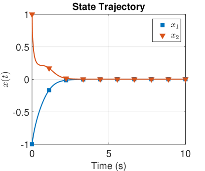
Figure 1: State trajectories generated using StaF kernel-based ADP.

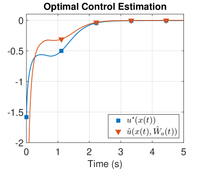
Figure 2: Control trajectory generated using StaF kernel-based ADP compared with the optimal control trajectory.

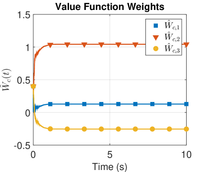
Figure 3: Trajectories of the estimates of the unknown parameters in the value function generated using StaF kernel-based ADP. The ideal weights are unknown and time-varying; hence, the obtained weights can not be compared with their ideal weights.

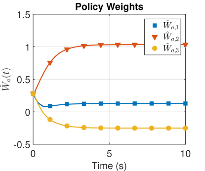
Figure 4: Trajectories of the estimates of the unknown parameters in the policy generated using StaF kernel-based ADP. The ideal weights are unknown and time-varying; hence, the obtained weights can not be compared with their ideal weights.

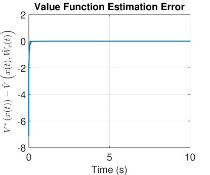
Figure 5: The error between the optimal and the estimated value function.

Figure 1 shows that the developed StaF-based controller drives the system states to the origin while maintaining system stability. Figure 2 shows the implemented control signal compared with the optimal control signal. It is clear that the implemented control converges to the optimal controller. Figure 3 shows that the weight estimates for the StaF-based value function and policy approximation remain bounded and converge as the state converges to the origin. Since the ideal values of the weights are unknown, the weights can not directly be compared with their ideal values. However, since the optimal solution is known, the value function estimate corresponding to the weights in Figure 3 can be compared to the optimal value function at each time $t$. Figure 5 shows that the error between the optimal and the estimated value functions rapidly decays to zero.

V-B Optimal tracking problem with parametric uncertainties in the drift dynamics

V-B1 Simulation parameters

Similar to [20], the developed StaF-based RL technique is extended to solve optimal tracking problems with parametric uncertainties in the drift dynamics. The drift dynamics in the two-dimensional nonlinear dynamical system in (30) are assumed to be linearly parameterized as

$$f\left(x^{o}\right)=\underset{\theta^{T}}{\underbrace{\left[\begin{array}[]{ccc}\theta_{1}&\theta_{2}&\theta_{3}\\ \theta_{4}&\theta_{5}&\theta_{6}\end{array}\right]}}\underset{\sigma_{\theta}\left(x^{o}\right)}{\underbrace{\left[\begin{array}[]{c}x_{1}^{o}\\ x_{2}^{o}\\ x_{2}^{o}\left(cos\left(2x_{1}^{o}\right)+2\right)\end{array}\right]}},$$

where $\theta\in\mathbb{R}^{3\times 2}$ is the matrix of unknown parameters and $\sigma_{\theta}$ is the known vector of basis functions. The ideal values of the unknown parameters are $\theta_{1}=-1$, $\theta_{2}=1$, $\theta_{3}=0$, $\theta_{4}=-0.5$, $\theta_{5}=0$, and $\theta_{6}=-0.5$. Let $\hat{\theta}$ denote an estimate of the unknown matrix $\theta.$ The control objective is to drive the estimate $\hat{\theta}$ to the ideal matrix $\theta$, and to drive the state $x$ to follow a desired trajectory $x_{d}$. The desired trajectory is selected to be solution of the initial value problem

$$\dot{x}_{d}\left(t\right)=\begin{bmatrix}-1&1\\ -2&1\end{bmatrix}x_{d}\left(t\right),\quad x_{d}\left(0\right)=\begin{bmatrix}0\\ 1\end{bmatrix},$$ (32)

and the cost functional is selected to be $\intop_{0}^{\infty}\left(e^{T}\left(t\right)\mbox{diag}\left(10,\>10\right)e\left(t\right)+\left(\mu\left(t\right)\right)^{2}\right)dt$, where $e\left(t\right)=x\left(t\right)-x_{d}\left(t\right),$ $\mu\left(t\right)=u\left(t\right)-g^{+}\left(x_{d}\left(t\right)\right)\left(\begin{bmatrix}-1&1\\ -2&1\end{bmatrix}x_{d}\left(t\right)-f\left(x_{d}\left(t\right)\right)\right)$, and $g^{+}\left(x^{o}\right)$ denotes the pseudoinverse of $g\left(x^{o}\right)$.

The value function is a function of the concatenated state $\zeta\triangleq\begin{bmatrix}e^{T}&x_{d}^{T}\end{bmatrix}^{T}\in\mathbb{R}^{4}$. The value function is approximated using five exponential StaF kernels given by $\sigma_{i}\left(\zeta^{o},c_{i}^{o}\right)$, where the five centers are selected according to $c_{i}^{o}\left(\zeta^{o}\right)=\zeta^{o}+d_{i}\left(\zeta^{o}\right)$ to form a regular five dimensional simplex around the current state with $\nu^{o}\left(\zeta^{o}\right)\equiv 1$. Learning gains for system identification and value function approximation are selected as

$$\mbox{$\eta$}_{c1}=0.001,\>\eta_{c2}=2,\>\eta_{a1}=2,\>\eta_{a2}=0.001,$$

$$\beta=0.01,\>\nu=0.1,\>\nu_{2}=1,\>k=500,$$

$$\mbox{$\Gamma$}_{\theta}=I_{3},\>\Gamma\left(0\right)=50I_{5},\>k_{\theta}=20,$$

To implement BE extrapolation, a single state trajectory $\zeta_{i}$ is selected as $\zeta_{i}\left(\zeta^{o},t\right)=\zeta^{o}+a_{i}\left(t\right)$, where $a_{i}\left(t\right)$ is sampled at each $t$ from a uniform distribution over the a $2.1\times 2.1\times 2.1\times 2.1$ hypercube centered at the origin. The history stack required for CL contains ten points, and is recorded online using a singular value maximizing algorithm (cf. [17]), and the required state derivatives are computed using a fifth order Savitzky-Golay smoothing filter (cf. [30]).

The initial values for the state and the state estimate are selected to be $x\left(0\right)=[0,0]^{T}$ and $\hat{x}\left(0\right)=[0,0]^{T}$, respectively. The initial values for the NN weights for the value function, the policy, and the drift dynamics are selected to be $0.025\times\mathbf{1}_{5}$, $0.025\times\mathbf{1}_{5}$, and $\mathbf{0}_{3\times 2}$, respectively, where $\mathbf{0}_{3\times 2}$ denotes a $3\times 2$ matrix of zeros. Since the system in (30) has no stable equilibria, the initial policy $\hat{\mu}\left(\zeta,\mathbf{0}_{3\times 2}\right)$ is not stabilizing. The stabilization demonstrated in Figure 6 is achieved via fast simultaneous learning of the system dynamics and the value function.

V-B2 Results

Figures 6 and 7 demonstrate that the controller remains bounded and the tracking error is regulated to the origin. The NN weights are functions of the system state $\zeta$. Since $\zeta$ converges to a periodic orbit, the NN weights also converge to a periodic orbit (within the bounds of the excitation introduced by the BE extrapolation signal), as demonstrated in Figures 8 and 9. Figure 10 demonstrates that the unknown parameters in the drift dynamics, represented by solid lines, converge to their ideal values, represented by dashed lines.

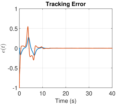
Figure 6: Tracking error trajectories generated using the proposed method for the nonlinear system.

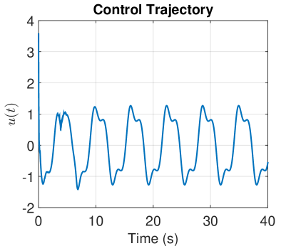
Figure 7: Control signal generated using the proposed method for the nonlinear system.

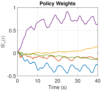
Figure 8: Policy weight trajectories generated using the proposed method for the nonlinear system. The weights do not converge to a steady-state value because the ideal weights are functions of the time-varying system state. Since an analytical solution of the optimal tracking problem is not available, weights cannot be compared against their ideal values

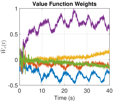
Figure 9: Value function weight trajectories generated using the proposed method for the nonlinear system. The weights do not converge to a steady-state value because the ideal weights are functions of the time-varying system state. Since an analytical solution of the optimal tracking problem is not available, weights cannot be compared against their ideal values

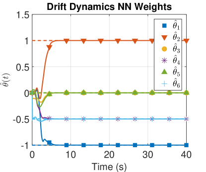
Figure 10: Trajectories of the unknown parameters in the system drift dynamics for the nonlinear system. The dotted lines represent the true values of the parameters.

V-C Comparison

Method	Running time (s)	Total cost	Steady-state RMS error
StaF kernels with single moving extrapolation points	0.95	2.82	$2.5\times 10^{-3}$
Technique developed in [19]	2	1.83	$6.15\times 10^{-6}$

Table I: Regulation simulation running times for the developed technique and the technique in [19]

Method	Running time (s)	Total cost	Steady-state RMS error
StaF kernels with single moving extrapolation points	15	6.38	$2.13\times 10^{-4}$
Technique developed in [20]	103	3.1	$2.7\times 10^{-4}$

Table II: Tracking simulation running times for the developed technique and the technique in [20]

The developed technique is compared with the model-based RL method developed in [19] for regulation and [20] for tracking, respectively. Both the simulations are performed in MATLAB^® SIMULINK^® at 1000 Hz on the same machine. The regulation simulations run for 10 seconds of simulated time, and the tracking simulations run for 40 seconds of simulated time. Tables I and II show that the developed controller requires significantly fewer computational resources than the controllers from [19] and [20].

Since the optimal solution for the regulation problem is known to be quadratic, the model-based RL method from [19] is implemented using three quadratic basis functions. Since the basis used is exact, the method from [19] yields a smaller steady-state error than the developed method, which uses three inexact, but generic StaF kernels. For the tracking problem, the method from [20] is implemented using ten polynomial basis functions selected based on a trial-and-error approach. The developed technique is implemented using five generic StaF kernels. In this case, since the optimal solution is unknown, both the methods use inexact basis functions, resulting in similar steady-state errors.

The two main advantages of StaF kernels are that they are universal, in the sense that they can be used to approximate a large class of value functions, and that they target local approximation, resulting in a smaller number of required basis functions. However, the StaF kernels trade optimality for universality and computational efficiency. The kernels are inexact, and the weight estimates need to be continually adjusted based on the system trajectory. Hence, as shown in Tables I and II, the developed technique results in a higher total cost than state-of-the-art model-based RL techniques.

VI Conclusion

In this paper an infinite horizon optimal control problem is solved using a new approximation methodology called the StaF kernel method. Motivated by the fact that a smaller number of basis functions is required to approximate functions on smaller domains, the StaF kernel method aims to maintain good approximation of the value function over a small neighborhood of the current state. Computational efficiency of model-based RL is improved by allowing selection of fewer time-varying extrapolation trajectories instead of a large number of autonomous extrapolation functions. Simulation results are presented that solve the infinite horizon optimal regulation and tracking problems online for a two state system using only three and five basis functions, respectively, via the StaF kernel method.

State-of-the-art solutions to solve infinite horizon optimal control problems online aim to approximate the value function over the entire operating domain. Since the approximate optimal policy is completely determined by the value function estimate, state-of-the-art solutions generate policies that are valid over the entire state space. Since the StaF kernel method aims at maintaining local approximation of the value function around the current system state, the StaF kernel method lacks memory, in the sense that the information about the ideal weights over a region of interest is lost when the state leaves the region of interest. Thus, unlike existing techniques, the StaF method generates a policy that is near-optimal only over a small neighborhood of the origin. A memory-based modification to the StaF technique that retains and reuses past information is a subject for future research.

References

• [1] R. S. Sutton and A. G. Barto, Reinforcement Learning: An Introduction.   Cambridge, MA, USA: MIT Press, 1998.
• [2] D. Bertsekas, Dynamic Programming and Optimal Control.   Athena Scientific, 2007.
• [3] P. Mehta and S. Meyn, “Q-learning and pontryagin’s minimum principle,” in Proc. IEEE Conf. Decis. Control, Dec. 2009, pp. 3598 –3605.
• [4] K. Doya, “Reinforcement learning in continuous time and space,” Neural Comput., vol. 12, no. 1, pp. 219–245, 2000.
• [5] R. Padhi, N. Unnikrishnan, X. Wang, and S. Balakrishnan, “A single network adaptive critic (SNAC) architecture for optimal control synthesis for a class of nonlinear systems,” Neural Netw., vol. 19, no. 10, pp. 1648–1660, 2006.
• [6] A. Al-Tamimi, F. L. Lewis, and M. Abu-Khalaf, “Discrete-time nonlinear HJB solution using approximate dynamic programming: Convergence proof,” IEEE Trans. Syst. Man Cybern. Part B Cybern., vol. 38, pp. 943–949, 2008.
• [7] F. L. Lewis and D. Vrabie, “Reinforcement learning and adaptive dynamic programming for feedback control,” IEEE Circuits Syst. Mag., vol. 9, no. 3, pp. 32–50, 2009.
• [8] T. Dierks, B. Thumati, and S. Jagannathan, “Optimal control of unknown affine nonlinear discrete-time systems using offline-trained neural networks with proof of convergence,” Neural Netw., vol. 22, no. 5-6, pp. 851–860, 2009.
• [9] K. Vamvoudakis and F. Lewis, “Online actor-critic algorithm to solve the continuous-time infinite horizon optimal control problem,” Automatica, vol. 46, no. 5, pp. 878–888, 2010.
• [10] H. Zhang, L. Cui, X. Zhang, and Y. Luo, “Data-driven robust approximate optimal tracking control for unknown general nonlinear systems using adaptive dynamic programming method,” IEEE Trans. Neural Netw., vol. 22, no. 12, pp. 2226–2236, 2011.
• [11] S. Bhasin, R. Kamalapurkar, M. Johnson, K. Vamvoudakis, F. L. Lewis, and W. Dixon, “A novel actor-critic-identifier architecture for approximate optimal control of uncertain nonlinear systems,” Automatica, vol. 49, no. 1, pp. 89–92, 2013.
• [12] H. Zhang, L. Cui, and Y. Luo, “Near-optimal control for nonzero-sum differential games of continuous-time nonlinear systems using single-network adp,” IEEE Trans. Cybern., vol. 43, no. 1, pp. 206–216, 2013.
• [13] H. Zhang, D. Liu, Y. Luo, and D. Wang, Adaptive Dynamic Programming for Control Algorithms and Stability, ser. Communications and Control Engineering.   London: Springer-Verlag, 2013.
• [14] K. Vamvoudakis and F. Lewis, “Online synchronous policy iteration method for optimal control,” in Recent Advances in Intelligent Control Systems, W. Yu, Ed.   Springer, 2009, pp. 357–374.
• [15] G. Chowdhary, “Concurrent learning adaptive control for convergence without persistencey of excitation,” Ph.D. dissertation, Georgia Institute of Technology, December 2010.
• [16] G. Chowdhary and E. Johnson, “A singular value maximizing data recording algorithm for concurrent learning,” in Proc. American Control Conf., 2011, pp. 3547–3552.
• [17] G. Chowdhary, T. Yucelen, M. Mühlegg, and E. N. Johnson, “Concurrent learning adaptive control of linear systems with exponentially convergent bounds,” Int. J. Adapt. Control Signal Process., vol. 27, no. 4, pp. 280–301, 2013.
• [18] H. Modares, F. L. Lewis, and M.-B. Naghibi-Sistani, “Integral reinforcement learning and experience replay for adaptive optimal control of partially-unknown constrained-input continuous-time systems,” Automatica, vol. 50, no. 1, pp. 193–202, 2014.
• [19] R. Kamalapurkar, P. Walters, and W. E. Dixon, “Concurrent learning-based approximate optimal regulation,” in Proc. IEEE Conf. Decis. Control, Florence, IT, Dec. 2013, pp. 6256–6261.
• [20] R. Kamalapurkar, L. Andrews, P. Walters, and W. E. Dixon, “Model-based reinforcement learning for infinite-horizon approximate optimal tracking,” in Proc. IEEE Conf. Decis. Control, 2014.
• [21] R. Kamalapurkar, J. Klotz, and W. Dixon, “Concurrent learning-based online approximate feedback Nash equilibrium solution of N -player nonzero-sum differential games,” Acta Automatica Sinica, to appear.
• [22] B. Luo, H.-N. Wu, T. Huang, and D. Liu, “Data-based approximate policy iteration for affine nonlinear continuous-time optimal control design,” Automatica, 2014.
• [23] X. Yang, D. Liu, and Q. Wei, “Online approximate optimal control for affine non-linear systems with unknown internal dynamics using adaptive dynamic programming,” IET Control Theory Appl., vol. 8, no. 16, pp. 1676–1688, 2014.
• [24] J. A. Rosenfeld, R. Kamalapurkar, and W. E. Dixon, “State following (StaF) kernel functions for function approximation part i: Theory and motivation,” in Proc. Am. Control Conf., 2015, to appear.
• [25] G. G. Lorentz, Bernstein polynomials, 2nd ed.   Chelsea Publishing Co., New York, 1986.
• [26] D. Kirk, Optimal Control Theory: An Introduction.   Dover, 2004.
• [27] D. Liberzon, Calculus of variations and optimal control theory: a concise introduction.   Princeton University Press, 2012.
• [28] P. Ioannou and J. Sun, Robust Adaptive Control.   Prentice Hall, 1996.
• [29] H. K. Khalil, Nonlinear Systems, 3rd ed.   Upper Saddle River, NJ, USA: Prentice Hall, 2002.
• [30] A. Savitzky and M. J. E. Golay, “Smoothing and differentiation of data by simplified least squares procedures.” Anal. Chem., vol. 36, no. 8, pp. 1627–1639, 1964.