OpTHyLiC: an Optimised Tool for Hybrid Limits Computation

Abstract

A software tool, computing observed and expected upper limits on Poissonian process rates using a hybrid frequentist-Bayesian $CL_{s}$ method, is presented. This tool can be used for simple counting experiments where only signal, background and observed yields are provided or for multi-bin experiments where binned distributions of discriminating variables are provided. It allows the combination of several channels and takes into account statistical and systematic uncertainties, as well as correlations of systematic uncertainties between channels. It has been validated against other software tools and analytical calculations, for several realistic cases.

1 Introduction

In a physics experiment, the result must sometimes be interpreted in terms of upper limits on the rate of a particular physical process of interest, dubbed signal. OpTHyLiC offers an easy-to-use hybrid frequentist-Bayesian solution to set upper limits for an arbitrary number of channels and backgrounds, using the $CL_{s}$ method. It can be used for simple counting experiments where only signal, background and observed yields are provided as well as for multi-bin experiments where binned distributions of discriminating variables are provided. Statistical and systematic uncertainties are taken into account in a Bayesian way, and correlations of systematic uncertainties across backgrounds and channels are properly accounted for. OpTHyLiC can be downloaded from [1].

Other tools such as McLimit [2] or RooStats [3] provide the ability to compute limits using the hybrid method. However, OpTHyLiC was specifically optimized for this method: it is lightweight, simple and faster than the tools most often used currently (even in complex cases with many backgrounds, channels and nuisance parameters, limits are typically computed in one minute or less). Furthermore, it provides several options to configure the treatment of statistical and systematic uncertainties. OpTHyLiC does not support profiling of uncertainties; the motivations for this choice are discussed in the next section.

The document is organized as follows. Typical situations in which OpTHyLiC can be used are described in Sec. 2. The notations used in this paper are introduced in Sec. 3. The statistical method implemented in OpTHyLiC is described in Sec. 4. The software is described in Sec. 5 and its validation in Sec. 6.

2 Purpose of the software

The OpTHyLiC software was written in order to provide users with a lightweight, simple and fast tool to compute upper limits. It should be seen as a complementary tool to the several existing ones. Because of the absence of profiling, it does not provide the best upper limits in cases where data capable of strongly constraining nuisance parameters exist. In such cases, users should prefer other tools like pure frequentist ones (which implement profiling of uncertainties) or pure Bayesian ones. OpTHyLiC is more specifically dedicated to situations where no such data exist or to situations where pure frequentist or pure Bayesian tools are too slow for the users’ needs. In the former situation, it is often observed that pure frequentist, pure Bayesian and hybrid approaches yield similar limits. It can therefore be advantageous to use OpTHyLiC rather than tools that are more complicated to handle and slower. The latter situation occurs for example when the expected number of events is small and asymptotic properties of the profile likelihood ratio can’t be used to speed up pure frequentist calculations (in this case pseudo-experiments must be drawn in order to perform the hypothesis tests which can be very time consuming when profiling a large number uncertainties). It can also occur when the aim is rather to perform an optimisation of the analysis (to determine the best event selection criteria or the best histogram binning for instance) than to compute final limits. Such optimisation studies often do not require high accuracy and can be extremely time consuming or even impossible to do with profiling.

OpTHyLiC can be used by physicists needing a tool relatively easy to master that provides reliable results taking into account several analysis channels and/or systematic uncertainties. It can for example be useful to perform phenomenological sensitivity studies or to recast published searches with newer theoretical models.

OpTHyLiC can also be used by beginners in statistics willing to perform limit calculations in realistic cases for the first time without having to understand first all the details and subtleties of profiling in pure frequentist calculations. Those aiming at understanding the details and subtleties of pure frequentist calculations can also use OpTHyLiC as an intermediate step towards that final objective. Many of the quantities, definitions and concepts presented in this paper and used in OpTHyLiC are indeed also used by tools like HistFactory and RooStats to perform pure frequentist calculations. Even though OpTHyLiC was originally designed for high energy physics it can also be used in other fields such as nuclear measurements or medical physics. Many measurements performed in such fields are poissonian and can be modelled with the OpTHyLiC statistical model. OpTHyLiC can therefore be used to perform statistical inference and gain valuable informations about physics parameters relevant in those fields too.

3 Notations and definitions

The following notations will be used throughout the document:

• $\mu$: signal strength modifier, defined as the tested signal rate divided by a fixed reference signal rate value (such as obtained from a theoretical prediction);

• $\mu_{\text{up}}$: upper limit on the signal strength modifier;

• $n$: number of channels;

• $s_{c\theta}$: event yield for signal process in channel $c$ ($c\in[1,n]$) and bin $\theta$;

• $s_{c\theta}^{\text{nom}}$: nominal reference event yield for signal process in channel $c$ and bin $\theta$;

• $\sigma_{cl}$: absolute systematic uncertainty for signal process in channel $c$ and bin $\theta$, due to the finite size of the control sample;

• $b_{ci\theta}$: event yield for type $i$ background process in channel $c$ and bin $\theta$;

• $b_{ci\theta}^{\text{nom}}$: nominal event yield for type $i$ background process in channel $c$ and bin $\theta$;

• $b_{c\theta}^{\text{nom}}=\sum\limits_{i\in\mathrm{backgrounds}}b_{ci\theta}^{\text{nom}}$: total nominal yield for background processes in channel $c$ and bin $\theta$;

• $\sigma_{ci\theta}$: absolute systematic uncertainty for type $i$ background process in channel $c$ and bin $\theta$, due to the finite size of the control sample;

• $N_{c\theta}$: event yield in channel $c$ and bin $\theta$;

• $N^{\text{obs}}_{c\theta}$: event yield actually observed in the data or the pseudo-data in channel $c$ and bin $\theta$.

A channel corresponds to a region enriched in signal events (also called signal region). In the case of multi-bin experiments, the user must provide binned distributions (or histograms) for each channel, background and signal. Bins of these distributions are referred to by the index $\theta$. For counting experiments, only yields for each background and signal in each channel are needed. In this case, the index $\theta$ is irrelevant and is discarded.

4 Method description

OpTHyLiC implements the $CL_{s}$ method [4]. Pseudo-experiments are generated and the distribution of a test statistic is determined under both signal plus background and background only hypotheses. From these distributions, $CL_{s}$ is computed and the upper limit on the signal strength modifier $\mu_{\text{up}}$ is found by solving the equation

$$CL_{s}\left(\mu\right)=\alpha,$$ (1)

for a fixed value of $\alpha$ which is set depending on the chosen confidence level $1-\alpha$. For 95% confidence level upper limits, $\alpha=0.05$. The test statistic used is the ratio of likelihoods under signal plus background and background only hypotheses:

$$q_{\mu}=-2\ln\frac{{{\cal L}}(\mu)}{{\cal L}(\mu=0)}.$$ (2)

The general form of the likelihood is discussed in Sec. 4.1. The statistical and systematic uncertainties are included by the use of nuisance parameters, as detailed in Sec. 4.2 and 4.3, respectively. These uncertainties are accounted for in a Bayesian way: the inference of the observed upper limit is performed from pseudo-experiments using the distribution of the likelihood marginalised over the nuisance parameters, as explained in Sec. 4.4. The procedure for calculating the expected limits is summarised in Sec. 4.5.

4.1 Statistical model

The full likelihood, including all nuisance parameters, is given by:

$$\begin{array}[]{rl}{\cal L}(\mu,\{s_{c\theta}^{\prime},b_{ci\theta}^{\prime},\eta_{j}\})=\prod\limits_{c,\theta}&\left[\frac{\left(\mu s_{c\theta}+b_{c\theta}\right)^{N_{c\theta}}}{N_{c\theta}!}e^{-\left(\mu s_{c\theta}+b_{c\theta}\right)}\right.\\ &\times f\left(s_{c\theta}^{\prime};s_{c\theta}^{\text{nom}},\sigma_{c\theta}\right)\prod\limits_{i}f\left(b_{ci\theta}^{\prime};b_{ci\theta}^{\text{nom}},\sigma_{ci\theta}\right)\left.\vphantom{\frac{\left(\mu s_{c\theta}+b_{c\theta}\right)^{N_{c\theta}}}{N_{c\theta}!}}\right]\prod\limits_{j}g\left(\eta_{j}\right),\\ \end{array}$$ (3)

where:

• the index $c$ runs over the channels;

• the index $i$ runs over the backgrounds;

• the index $\theta$ runs over the bins;

• the index $j$ runs over the systematic uncertainties;

• $s_{c\theta}=s_{c\theta}^{\prime}\times k_{c\theta}^{\text{syst}}\left(\{\eta_{j}\}\right)$;

• $b_{c\theta}=\sum\limits_{i\in\text{backgrounds}}b_{ci\theta}=\sum\limits_{i\in\text{backgrounds}}b_{ci\theta}^{\prime}\times k_{ci\theta}^{\text{syst}}\left(\{\eta_{j}\}\right)$.

In OpTHyLiC, the signal always adds to the background ($\mu s_{c\theta}$ is always positive). Cases where the searched signal causes a deficit of events with respect to the background only hypothesis therefore can’t be treated with OpTHyLiC.

The set of nuisance parameters $\{s_{c\theta}^{\prime},b_{ci\theta}^{\prime},\eta_{j}\}$ can be divided into two categories. The first ones, $\{s_{c\theta}^{\prime},b_{ci\theta}^{\prime}\}$, account for the systematic uncertainties due to the finite size of the control samples used to estimate the signal and background nominal yields $s_{c\theta}^{\text{nom}}$ and $b_{ci\theta}^{\text{nom}}$, respectively. Such uncertainties are referred to as “statistical uncertainties” in this paper. These nuisance parameters are constrained by the functions $f$. The second ones, $\{\eta_{j}\}$, account for the systematic uncertainties. They are constrained by the functions $g$. The variation of the signal and background yields under the effect of the systematic uncertainties are described by the functions $k_{c\theta}^{\text{syst}}\left(\{\eta_{j}\}\right)$ and $k_{ci\theta}^{\text{syst}}\left(\{\eta_{j}\}\right)$, respectively.

Bins of discriminating variable histograms are treated as channels: the drawing of Poisson random numbers and the statistical uncertainties on the yield of each process in each bin are independent, but a given systematic uncertainty may affect the yields in a correlated way. It is therefore equivalent to run a counting experiment with $N$ channels and a binned experiment with $N$ bins where the yields and uncertainties in each bin match those in the channels.

4.2 Treatment of statistical uncertainties

The nuisance parameters $s_{c}^{\prime}$ and $b_{ci}^{\prime}$, accounting for the statistical uncertainties on the nominal signal and background yields, are constrained by probability density functions (p. d. f.) $f$ of the form:

$$f(y;y^{\text{nom}},\sigma),$$ (4)

where $y$ is the nuisance parameter, $y^{\text{nom}}$ the nominal yield and $\sigma$ the statistical uncertainty, which can be the square root of summed squared weights (e.g. when $y^{\text{nom}}$ is estimated from a mixture of normalised simulated samples).

In OpTHyLiC, five different p. d. f. can be used as constraints: a normal distribution, a log-normal distribution, or three different types of gamma distributions.

4.2.1 Normal and log-normal constraints

The parameters of the normal and log-normal p. d. f. are chosen so that the average and the standard deviation of these distributions are equal to $y^{\text{nom}}$ and $\sigma$, respectively. The normal distribution has the form:

$$f_{\text{N}}(y;y^{\text{nom}},\sigma)=\frac{1}{\sigma\sqrt{2\pi}}\exp\left(-\frac{(y-y^{\text{nom}})^{2}}{2\sigma^{2}}\right),$$ (5)

and the log-normal distribution has the form:

$$f_{\text{L}}(y;y^{\text{nom}},\sigma)=\frac{1}{y\ b\sqrt{2\pi}}\exp\left(-\frac{(\ln y-a)^{2}}{2b^{2}}\right),$$ (6)

with:

$$a=\ln\left(\frac{\left(y^{\text{nom}}\right)^{2}}{\sqrt{\left(y^{\text{nom}}\right)^{2}+\sigma^{2}}}\right)\text{and}\ b=\sqrt{\ln\left(1+\frac{\sigma^{2}}{\left(y^{\text{nom}}\right)^{2}}\right)}.$$ (7)

The normal distribution can be defined for any real $y$ values, including non-physical negative event yields. On the contrary, the log-normal distribution is defined only for $y>0$.

In the log-normal case, the nominal yield $y^{\text{nom}}$ and statistical uncertainty $\sigma$ estimated by users are interpreted as the average and standard deviation of the distribution, respectively. However, a different interpretation is possible. For example, if the statistical uncertainty results from a maximum likelihood estimate on some auxiliary dataset, $y^{\text{nom}}$ corresponds to the mode of the likelihood and $\sigma$ to the uncertainty as measured from the curvature of the log-likelihood around the mode ($\sigma=-1/\sqrt{\left(\ln f_{\text{L}}\right)^{{}^{\prime\prime}}\left(y=y^{\text{nom}}\right)}$). The parameters $a$ and $b$ of the log-normal distribution should therefore be equal to:

$$a=\frac{\sigma^{2}}{\left(y^{\text{nom}}\right)^{2}}+\ln\left(y^{\text{nom}}\right)\text{and}\ b=\frac{\sigma}{y^{\text{nom}}}.$$ (8)

This can be achieved in OpTHyLiC by setting input parameters to:

$$e^{a+\frac{b^{2}}{2}}~{}\text{and}\ e^{a+\frac{b^{2}}{2}}\sqrt{e^{b^{2}}-1}~{}\text{,}$$ (9)

with $a$ and $b$ given by Eq. 8, rather than to $y^{\text{nom}}$ and $\sigma$, respectively.

4.2.2 Gamma constraints

Three gamma p. d. f. are implemented in OpTHyLiC. They have the general form:

$$f_{\text{G}}(y;a,b)=\frac{a\left(ay\right)^{b-1}e^{-ay}}{\Gamma\left(b\right)},$$ (10)

where $a$ and $b$ are the rate and shape parameters respectively. As for the log-normal, the gamma distributions are defined for any strictly positive value of $y$.

This p. d. f. can be seen as the posterior distribution obtained from an auxiliary measurement accounting for the Poissonian nature of the statistical uncertainty. Accounting for this nature is not straightforward since events are in general weighted. A popular approach (used for example in HistFactory [5]) is to consider an imaginary auxiliary measurement in which all events have unit weight (which can therefore be described by a Poisson distribution) and in which the relative statistical uncertainty is equal to that used in the main measurement ($\sigma/y^{\text{nom}}$).

Let $N_{\text{aux}}$ be the number of events observed in this auxiliary measurement. The auxiliary measurement likelihood is:

$$P(N_{\text{aux}};\lambda)=\frac{\lambda^{N_{\text{aux}}}}{\Gamma\left(N_{\text{aux}}+1\right)}e^{-\lambda},$$ (11)

where $\lambda$ is the (unknown) nuisance parameter. It can be written as:

$$\lambda=\gamma\ N_{\text{aux}}^{\text{nom}},$$ (12)

where $N_{\text{aux}}^{\text{nom}}$ is the nominal value of $N_{\text{aux}}$ and $\gamma$ the nuisance parameter affecting the yield in the main measurement – the product of Poisson terms in Eq. 3 – in a multiplicative way: $y=\gamma\ y^{\text{nom}}$. $N_{\text{aux}}^{\text{nom}}$ is found by imposing that the relative statistical uncertainty is the same in the auxiliary and main measurements:

$$N_{\text{aux}}^{\text{nom}}=\left(\frac{y^{\text{nom}}}{\sigma}\right)^{2}.$$ (13)

The auxiliary measurement likelihood can then be written as follows:

$$P(N_{\text{aux}};\gamma)=\frac{\left(\gamma\left(y^{\text{nom}}/\sigma\right)^{2}\right)^{N_{\text{aux}}}}{\Gamma\left(N_{\text{aux}}+1\right)}e^{-\gamma\left(y^{\text{nom}}/\sigma\right)^{2}}.$$ (14)

From this likelihood, posterior distributions for $\gamma$ can be determined for various prior distributions $\pi\left(\gamma\right)$:

$$g\left(\gamma\right)=\frac{P(N_{\text{aux}}=N_{\text{aux}}^{\text{nom}};\gamma)\pi\left(\gamma\right)}{\displaystyle\int P(N_{\text{aux}}=N_{\text{aux}}^{\text{nom}};\gamma)\pi\left(\gamma\right){\rm d}\gamma}.$$ (15)

These posterior distributions can then be translated into posterior distributions for the yield $y$ (hereafter denoted as $f(y;y^{\text{nom}},\sigma)$, using the same notation as in Eq. 4).

Three prior distributions are considered; in each case, the posterior distribution for $y$ is a gamma distribution with the general form given by Eq. 10:

• $\pi\left(\gamma\right)\propto 1$ (uniform prior); in this case, the posterior distribution is:

  $$f(y;y^{\text{nom}},\sigma)=f_{\text{G}}\left(y;a=y^{\text{nom}}/\sigma^{2},b=\left(y^{\text{nom}}/\sigma\right)^{2}+1\right);$$ (16a)

• $\pi\left(\gamma\right)\propto 1/\sqrt{\gamma}$ (Jeffreys prior); in this case, the posterior distribution is:

  $$f(y;y^{\text{nom}},\sigma)=f_{\text{G}}\left(y;a=y^{\text{nom}}/\sigma^{2},b=\left(y^{\text{nom}}/\sigma\right)^{2}+1/2\right);$$ (16b)

• $\pi\left(\gamma\right)\propto 1/\gamma$ (hyperbolic prior); in this case, the posterior distribution is:

  $$f(y;y^{\text{nom}},\sigma)=f_{\text{G}}\left(y;a=y^{\text{nom}}/\sigma^{2},b=\left(y^{\text{nom}}/\sigma\right)^{2}\right).$$ (16c)

The three gamma constraints available in OpTHyLiC correspond to the three posteriors given in Eq. 16a, 16b and 16c. Their parameters are summarized in Tab. 1.

prior	posterior parameters
	$a$	$b$
$\pi\left(\gamma\right)\propto 1$	$y^{\text{nom}}/\sigma^{2}$	$\left(y^{\text{nom}}/\sigma\right)^{2}+1$
$\pi\left(\gamma\right)\propto 1/\sqrt{\gamma}$	$y^{\text{nom}}/\sigma^{2}$	$\left(y^{\text{nom}}/\sigma\right)^{2}+1/2$
$\pi\left(\gamma\right)\propto 1/\gamma$	$y^{\text{nom}}/\sigma^{2}$	$\left(y^{\text{nom}}/\sigma\right)^{2}$

Table 1: Summary of the three gamma constraints available in OpTHyLiC. The constants $a$ and $b$ are parameters of the posterior distribution whose general form is given in Eq. 10.

4.2.3 Comparison of the constraint functions

The five available constraint functions – normal, log-normal and the three gamma distributions – are compared for three different values of $y^{\text{nom}}$ and $\sigma$ in Fig. 1. When $\sigma$ is small with respect to $y^{\text{nom}}$, the distributions are very close to each other. Otherwise, the differences between the distributions can be significant.

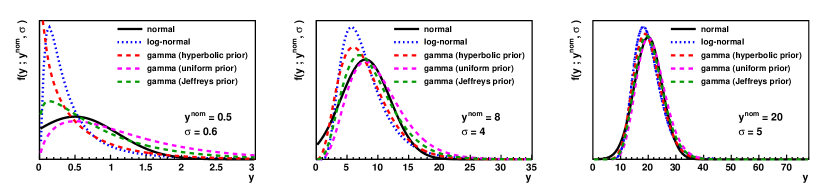
Figure 1: Comparison of normal, log-normal and gamma probability density functions used for statistical uncertainties for three values of $y^{\text{nom}}$ and $\sigma$.

Table 2 compares the mode, the expectation and standard deviation for the five available constraint functions. For the normal and log-normal distribution, the expectation and standard deviation are equal to the nominal yield and statistical uncertainty (see Sec. 4.2.1). For the gamma distributions the expectation and standard deviation are equal to the nominal yield and statistical uncertainty only for the hyperbolic prior $\pi\left(\gamma\right)\propto 1/\gamma$. For the gamma constraints with the uniform and Jeffreys priors, it is not the case, but the difference vanishes in the asymptotic limit.

distribution	mode	$\mathbb{E}\left[y\right]$	${\rm var}\left[y\right]$
normal	$y^{\text{nom}}$	$y^{\text{nom}}$	$\sigma^{2}$
log-normal	$y^{\text{nom}}\left(1+\left(\frac{\sigma}{y^{\text{nom}}}\right)^{2}\right)^{-3/2}$	$y^{\text{nom}}$	$\sigma^{2}$
gamma	$y^{\text{nom}}$	$y^{\text{nom}}\left(1+\left(\frac{\sigma}{y^{\text{nom}}}\right)^{2}\right)$	$\sigma^{2}\left(1+\left(\frac{\sigma}{y^{\text{nom}}}\right)^{2}\right)$
(uniform prior)
gamma	$y^{\text{nom}}\left(1-\frac{1}{2}\left(\frac{\sigma}{y^{\text{nom}}}\right)^{2}\right)$	$y^{\text{nom}}\left(1+\frac{1}{2}\left(\frac{\sigma}{y^{\text{nom}}}\right)^{2}\right)$	$\sigma^{2}\left(1+\frac{1}{2}\left(\frac{\sigma}{y^{\text{nom}}}\right)^{2}\right)$
(Jeffreys prior)
gamma	$y^{\text{nom}}\left(1-\left(\frac{\sigma}{y^{\text{nom}}}\right)^{2}\right)$	$y^{\text{nom}}$	$\sigma^{2}$
(hyperbolic prior)

Table 2: Comparison of the mode, expectation, and standard deviation for the five constraints available in OpTHyLiC.

Care should be taken when statistical uncertainties are large compared with the nominal yields or when nominal yields are equal to zero. When statistical uncertainties are large, constraint p. d. f. can be truncated at zero in the normal case. In such cases, log-normal and gamma should be preferred. When nominal yields are equal to zero, log-normal and gamma are undefined. In such cases, OpTHyLiC automatically selects a normal constraint truncated at zero. In general, users are encouraged to study the stability of the limit calculations depending on the assumptions made in such circumstances.

4.3 Treatment of systematic uncertainties

Systematic uncertainties on nominal yields $s_{c\theta}^{\text{nom}}$ and $b_{ci\theta}^{\text{nom}}$ are accounted for by including the set of nuisance parameters $\{\eta_{j}\}$. They are assumed to be either 100% correlated or completely uncorrelated. The total number of nuisance parameters is therefore equal to the total number of independent systematic uncertainties, including all channels, backgrounds and signals. The correlation factor between two nuisance parameters $\eta_{j}$ and $\eta_{k}$ is given by the Kronecker symbol $\delta_{jk}$. The term constraining nuisance parameters in the likelihood can thus be factorized into the product of individual constraint terms. In Eq. 3, the nuisance parameter for each systematic uncertainty of index $j$ is constrained by a standard normal p. d. f. $g$ of the form:

$$g\left(\eta_{j}\right)=\frac{1}{\sqrt{2\pi}}e^{-\frac{\eta_{j}^{2}}{2}}.$$ (17)

As stated in Sec. 4.1, the effect of systematic uncertainties on the yield is described by relations of the form:

$$y=y^{\text{nom}}\times k^{\text{syst}}\left(\{\eta_{j}\}\right),$$ (18)

where $y$ is the varied yield, $y^{\text{nom}}$ the nominal yield and $k^{\text{syst}}\left(\{\eta_{j}\}\right)$ the function describing the variation of the yield with the set of nuisance parameters $\{\eta_{j}\}$. OpTHyLiC provides two different solutions for combining the effect of multiple nuisance parameters:

• additive:

  $$k^{\text{syst}}\left(\{\eta_{j}\}\right)-1=\sum\limits_{j\in\text{systematics}}\left[h^{\text{syst}}_{j}\left(\eta_{j}\right)-1\right];$$ (19a)

• multiplicative:

  $$k^{\text{syst}}\left(\{\eta_{j}\}\right)=\prod\limits_{j\in\text{systematics}}h^{\text{syst}}_{j}\left(\eta_{j}\right).$$ (19b)

In Eq. 19a and 19b, $h^{\text{syst}}_{j}\left(\eta_{j}\right)$ is the function describing the variation of the yield with nuisance parameter $j$. In both cases, when the effect of only one nuisance parameter is considered, $k^{\text{syst}}\left(\eta_{j}\right)=h^{\text{syst}}_{j}\left(\eta_{j}\right)$ as it should.

For each systematic uncertainty $j$, the corresponding nuisance parameter $\eta_{j}$ is chosen such that $\eta_{j}=0$ corresponds to no variation, $\eta_{j}=+1$ to a $+1\sigma$ variation, and $\eta_{j}=-1$ to a $-1\sigma$ variation. The main issue associated to systematic uncertainties is the choice of the function $h^{\text{syst}}_{j}\left(\eta_{j}\right)$ that relates the effect of the systematic uncertainty to its associated nuisance parameter. Usually, $h^{\text{syst}}_{j}$ is known, for each systematic, for $\eta_{j}=0,-1$ and $+1$. The value of $h_{j}^{\mathrm{sys}}$ for $\eta_{j}=0$ is by definition equal to 1: it corresponds to the case $y=y^{\text{nom}}$. Let $h^{\uparrow}_{j}$ ($h^{\downarrow}_{j}$) be the relative variation of the yield when systematic $j$ is varied by $+1$ ($-1$) $\sigma$. Thus, for all $j$:

$$h^{\text{syst}}_{j}\left(\eta_{j}=0\right)=1;$$ (20a)

$$h^{\uparrow}_{j}=h^{\text{syst}}_{j}\left(\eta_{j}=+1\right)-1;$$ (20b)

$$h^{\downarrow}_{j}=h^{\text{syst}}_{j}\left(\eta_{j}=-1\right)-1.$$ (20c)

The problem consists in finding continuous functions $h^{\text{syst}}_{j}\left(\eta_{j}\right)$, interpolating for $\eta_{j}\in\left[-1,+1\right]$ and extrapolating for $\eta_{j}>+1$ and $\eta_{j}<-1$, and such that Eqs. 20 are satisfied – at least approximately. Four choices are currently available in OpTHyLiC, and are represented in Fig. 2:

• piece-wise linear interpolation and extrapolation, defined in Sec. 4.3.1;

• piece-wise exponential interpolation and extrapolation, defined in Sec. 4.3.2;

• polynomial interpolation and exponential extrapolation, defined in Sec. 4.3.3;

• “McLimit” interpolation and extrapolation, defined in Sec. 4.3.4 and corresponding to the choice followed in the McLimit program.

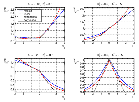
Figure 2: Illustration of interpolation and extrapolation functions implemented in OpTHyLiC for $h^{\downarrow}_{j}=-0.03$ and $h^{\uparrow}_{j}=0.5$ (top left), $h^{\downarrow}_{j}=-0.5$ and $h^{\uparrow}_{j}=0.5$ (top right), $h^{\downarrow}_{j}=0.2$ and $h^{\uparrow}_{j}=-0.5$ (bottom left) and $h^{\downarrow}_{j}=-0.5$ and $h^{\uparrow}_{j}=-0.5$ (bottom right).

4.3.1 Piece-wise linear interpolation and extrapolation

The piece-wise linear interpolation and extrapolation is defined as follows:

$$h^{\text{syst}}_{j}\left(\eta_{j}\right)=\left\{\begin{matrix}1+\eta_{j}h^{\uparrow}_{j}\quad\text{if $\eta_{j}$ is positive};\vspace*{0.15cm}\\ 1-\eta_{j}h^{\downarrow}_{j}\quad\text{if $\eta_{j}$ is negative}.\end{matrix}\right.$$ (21)

From this definition, it appears that $h^{\text{syst}}_{j}$ can be negative if $h^{\uparrow}_{j}$ or $h^{\downarrow}_{j}$ is negative. This unphysical behaviour is dealt with in OpTHyLiC by setting $h^{\text{syst}}_{j}$ to zero when it occurs.

4.3.2 Piece-wise exponential interpolation and extrapolation

The piece-wise exponential interpolation and extrapolation is defined as follows:

$$h^{\text{syst}}_{j}\left(\eta_{j}\right)=\left\{\begin{matrix}\left(1+h^{\uparrow}_{j}\right)^{\eta_{j}}\quad\text{if $\eta_{j}$ is positive},\vspace*{0.15cm}\\ \left(1+h^{\downarrow}_{j}\right)^{-\eta_{j}}\quad\text{if $\eta_{j}$ is negative}.\end{matrix}\right.$$ (22)

From this definition, it appears that $h^{\text{syst}}_{j}$ can be negative if $h^{\uparrow}_{j}$ or $h^{\downarrow}_{j}$ is lower than -1. This unphysical behaviour is dealt with in OpTHyLiC by applying a linear interpolation and extrapolation instead (see Sec. 4.3.1) when it occurs. If both $h^{\uparrow}_{j}$ and $h^{\downarrow}_{j}$ are greater than -1, $h^{\text{syst}}_{j}$ is positive for all $\eta_{j}$ values.

4.3.3 Polynomial interpolation and exponential extrapolation

The polynomial interpolation and exponential extrapolation is defined as follows:

$$h^{\text{syst}}_{j}\left(\eta_{j}\right)=\left\{\begin{matrix}\left(1+h^{\uparrow}_{j}\right)^{\eta_{j}}\quad\text{if $\eta_{j}\geq 1$},\vspace*{0.15cm}\\ 1+\sum\limits_{i=1}^{6}a_{i}\eta_{j}^{i}\quad\text{if $-1<\eta_{j}<1$},\vspace*{0.15cm}\\ \left(1+h^{\downarrow}_{j}\right)^{-\eta_{j}}\quad\text{if $\eta_{j}\leq-1$},\end{matrix}\right.$$ (23)

where the coefficients $a_{i}$ are chosen such that $h^{\text{syst}}_{j}\left(\eta_{j}\right)$ and its first and second derivatives are continuous at $|\eta_{j}|=1$ and $\eta_{j}=0$.

4.3.4 “McLimit” interpolation and extrapolation

The “McLimit” interpolation and extrapolation is defined as follows:

$$h^{\text{syst}}_{j}\left(\eta_{j}\right)=\left\{\begin{matrix}1+B\quad\text{if $B\geq 0$},\vspace*{0.15cm}\\ e^{B}\quad\text{if $B<0$},\end{matrix}\right.$$ (24)

where:

$$B=\left\{\begin{matrix}\eta_{j}h^{\uparrow}_{j}\left(1-R\right)+RQ\quad\text{if $\eta_{j}$ is positive},\vspace*{0.15cm}\\ -\eta_{j}h^{\downarrow}_{j}\left(1-R\right)+RQ\quad\text{if $\eta_{j}$ is negative},\end{matrix}\right.$$ (25)

$$Q=\eta_{j}\frac{h^{\uparrow}_{j}-h^{\downarrow}_{j}}{2}+\eta_{j}^{2}\frac{h^{\uparrow}_{j}+h^{\downarrow}_{j}}{2}\quad\text{and}\quad R=\frac{1}{1+3|\eta_{j}|}.$$ (26)

This definition ensures that the first derivative of $h^{\text{syst}}_{j}$ at $\eta_{j}=0$ is continuous and that $h^{\text{syst}}_{j}>0$ for all $\eta_{j}$ values. Equation 20b (20c) is exactly satisfied when $h^{\uparrow}_{j}>0$ ($h^{\downarrow}_{j}>0$) but only to first order when $h^{\uparrow}_{j}<0$ ($h^{\downarrow}_{j}<0$). Indeed, the following relations hold:

$$h^{\text{syst}}_{j}\left(\eta_{j}=+1\right)=\left\{\begin{matrix}e^{h^{\uparrow}_{j}}\quad\text{if}\quad h^{\uparrow}_{j}<0,\vspace*{0.15cm}\\ 1+h^{\uparrow}_{j}\quad\text{if}\quad h^{\uparrow}_{j}\geq 0,\end{matrix}\right.$$ (27)

$$h^{\text{syst}}_{j}\left(\eta_{j}=-1\right)=\left\{\begin{matrix}e^{h^{\downarrow}_{j}}\quad\text{if}\quad h^{\downarrow}_{j}<0,\vspace*{0.15cm}\\ 1+h^{\downarrow}_{j}\quad\text{if}\quad h^{\downarrow}_{j}\geq 0.\end{matrix}\right.$$ (28)

Also, when the effect of the considered uncertainty is symmetric ($h^{\uparrow}_{j}=-h^{\downarrow}_{j}$), this interpolation/extrapolation scheme is equivalent to the piece-wise linear one (see Sec. 4.3.1) for $\eta_{j}>0$ if $h^{\uparrow}\geq 0$ or $\eta_{j}<0$ if $h^{\downarrow}\geq 0$.

4.4 Inference of observed upper limit $\mu_{\text{up}}$

The observed upper limit on the signal strength $\mu_{\text{up}}$ is derived from the $CL_{s}$ method using $q_{\mu}$ (Eq. 2) as test statistic. $q_{\mu}$ is computed using the nominal likelihood:

$${\cal L}(\mu)={\cal L}(\mu,\{s_{c\theta}^{\prime}\}=\{s_{c\theta}^{\text{nom}}\},\{b_{ci\theta}^{\prime}\}=\{b_{ci\theta}^{\text{nom}}\},\{\eta_{j}\}=0).$$ (29)

It thus reduces to the following simple form:

$$q_{\mu}=\sum\limits_{c,\theta}q_{\mu}^{c\theta},$$ (30)

where $q_{\mu}^{c\theta}$ is the test for channel $c$ and bin $\theta$ given by:

$$q_{\mu}^{c\theta}=2\left(\mu s_{c\theta}^{\text{nom}}-N_{c\theta}\ln\frac{\mu s_{c\theta}^{\text{nom}}+b_{c\theta}^{\text{nom}}}{b_{c\theta}^{\text{nom}}}\right).$$ (31)

The distributions of $q_{\mu}$ under signal plus background and background only hypotheses (hereafter denoted as $p(q_{\mu}|\mu)$ and $p(q_{\mu}|0)$ respectively) are determined by generating pseudo-experiments from the marginal likelihood:

$${\cal L}_{\text{m}}\left(\mu\right)=\displaystyle\int{\cal L}(\mu,\{s_{c\theta}^{\prime},b_{ci\theta}^{\prime},\eta_{j}\})~{}\prod\limits_{j}{\rm d}\eta_{j}\prod\limits_{c,\theta}{\rm d}s_{c\theta}^{\prime}\prod\limits_{i}{\rm d}b_{ci\theta}^{\prime}.$$ (32)

In practice, this is done by first generating nuisance parameter values from their constraint p. d. f. and by then generating $N_{c\theta}$ using the nuisance parameter values obtained in the first step. Typical distributions produced by OpTHyLiC are shown in Fig. 3.

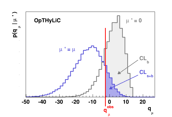
Figure 3: Example of distributions of $q_{\mu}$ under signal+background ($\mu^{\prime}=\mu$) and background only hypotheses ($\mu^{\prime}=0$).

Once $p(q_{\mu}|\mu)$ and $p(q_{\mu}|0)$ have been determined, $CL_{s}$ is computed by using:

$$CL_{s}\left(\mu\right)=\frac{CL_{s+b}}{CL_{b}}=\frac{\sum\limits_{q_{\mu}=q_{\mu}^{\text{obs}}}^{\infty}p(q_{\mu}|\mu)}{\sum\limits_{q_{\mu}=q_{\mu}^{\text{obs}}}^{\infty}p(q_{\mu}|0)},$$ (33)

where $q_{\mu}^{\text{obs}}$ is the observed value of the test ($q_{\mu}^{\text{obs}}=q_{\mu}\left(\{N_{c\theta}\}=\{N^{\text{obs}}_{c\theta}\}\right)$). The upper limit is found by searching $\mu$ such that $CL_{s}(\mu)$ is equal to $\alpha$ (see Eq. 1).

4.5 Computation of expected limits

OpTHyLiC can also be used to compute expected limits on the signal strength, under the background only hypothesis. Five expected limit quantiles are available: median, $-2\sigma$, $-1\sigma$, $+1\sigma$ and $+2\sigma$. The last four ones are defined using the standard normal distribution. Denoting these quantiles by $Z$ and the corresponding probability by $p$, one has:

$$Z=\Phi^{-1}\left(p\right),$$ (34)

where $\Phi$ is the cumulative distribution function of the standard normal distribution. The values of probabilities for the quantiles available in OpTHyLiC are given in Tab. 3.

$Z$	-2	-1	0 (median)	+1	+2
$p$	0.0228	0.1587	0.5	0.8413	0.9772

Table 3: Values of probabilities associated to the quantiles available in OpTHyLiC for the calculation of expected limits.

Two methods are provided to compute expected limits. In the first one, the distribution of $\mu_{\text{up}}$ is determined by generating pseudo-experiments under the background-only hypothesis. Expected limits are then given by the quantiles (as defined above) of this distribution. In the second one, expected limits are calculated in the same way as observed ones (see Sec. 4.4) replacing the observed $CL_{s}$ by median, $-2\sigma$, $-1\sigma$, $+1\sigma$ and $+2\sigma$ quantiles of the $CL_{s}$ distribution under background only hypothesis.

Both methods are equivalent from the statistical point of view but different in terms of implementation and computing time. In most cases, the second method performs much faster than the first one and should therefore be preferred. The first method can be used for cross-checks or if the distribution of $\mu_{\text{up}}$ is needed.

However, when using the second method, quantiles are not computed from a single distribution as in the first method: each quantile is computed in a separate job. Therefore, due to statistical fluctuations, the expected values may not be sorted as they should (for example, the $-2\sigma$ expected value can be higher than the $-1\sigma$ expected value). In such cases it is recommended to increase the number of pseudo-experiments.

5 Software description

5.1 Structure and prerequisites

OpTHyLiC is written in C++ and uses the ROOT library [6]. The code is separated in different classes. Their definitions and implementations are separated into different files which are placed in the main OpTHyLiC directory. Once compiled, the libraries can either be used dynamically by using a macro interpreted with the ROOT interpreter (CINT and CLING for version 5 and 6 of ROOT, respectively), or by using a C++ program compiled into an executable with a software like gcc. Two simple examples, working for both cases, are available in the examples sub-directory.

As the statistical method relies on pseudo-experiments, pseudo-random number generators are used. ROOT provides in its TRandom3 class an implementation of the MT19937 Mersenne twister [7]. The C++ standard library in its recent C++11 standard [8] also provides various pseudo-random number engines, which generate numbers distributed with the various probability distributions mentioned in this paper. Therefore, if the available compiler or ROOT version makes the use of the C++11 standard possible, the user has the possibility to chose these pseudo-random engines instead of the TRandom3 class. Thanks to relevant preprocessor directives, the portions of the code specific to the C++11 standard are ignored, either by the interpreter or by the compiler, when its use is not possible.

If used as a compiled executable, the examples have been tested to be fully functional with gcc version $4.8.2$ ($4.3.0$) or newer, with ROOT version $5.28/00\text{b}$, when C++11 features are (are not) used. If used as interpreted macros, the examples have been tested to be fully functional with ROOT versions as old as $6.02/03$ ($5.28/00\text{b}$), when C++11 features are (are not) used. Older versions of gcc and ROOT may also be used but have not been tested. Other compilers than gcc could also have been chosen, but have not been considered in the installation procedure described below.

The usage instructions given below corresponds to version $2.00$ of OpTHyLiC.

5.2 Installation and examples

OpTHyLiC is installed in three steps:

1. running the INSTALL script to prepare the compilation by creating a Makefile which structure depends on how OpTHyLiC is intended to be used;

2. running make to compile the shared libraries according to the Makefile;

3. running the setup.[c]sh script created in the first step, to update the LD_LIBRARY_PATH environment variable with the directory where the shared libraries are available.

The INSTALL shell script is in the main directory. Using INSTALL --help (or INSTALL -h) displays a help detailing the different options, which allows the user to configure the Makefile:

• --executable (or -e) to compile executables with gcc; if this option is not used, two ROOT macros, Compile.C and examples/load.C, needed for the compilation and for loading the shared libraries, are created in addition to the Makefile;

• --C++11 (or -C) to enable the C++11 features; in this case, the script checks if the gcc or ROOT versions are recent enough to do so;

• --permissive to override the check of the gcc or ROOT versions when using the previous option.

If no option is used, the libraries will be compiled by ROOT to be used with an interpreted macro, without the C++11 features. Once installed, OpTHyLiC can be used from any location when opening a new shell, by running the script setup.[c]sh.

Two examples of programs using OpTHyLiC, runLimits.C and runSignificance.C, are provided in the examples sub-directory, together with examples of input files "input1.dat", "input2.dat", "inputHistos.dat" and "inputHistosAlternativeSyntax.dat", the syntax of which is detailed in Sec. 5.3 ("input1.dat" and "input2.dat" illustrate the syntax for counting experiments and "inputHistos.dat" and "inputHistosAlternativeSyntax.dat" for multi-bin experiments). The example runLimits.C illustrates the calculation of expected and observed limits, while runSignificance.C shows how to plot the test statistic distribution under the background only and signal plus background hypotheses and calculate the observed and expected p-values and significances. The syntax of the main functions used in both examples is explained in Sec. 5.4.

These example programs can be run using the following syntax:

• root -l load.C ’runLimits.C("input1.dat",
"input2.dat")’
  when used as a ROOT macro;

• ./runLimits.exe --files input1.dat
input2.dat
  when used as an executable.

Here, files for counting experiments are provided. Files for multi-bin experiments are provided using exactly the same syntax (OpTHyLiC automatically recognises what type of input files are provided by the user and applies the right treatment in each case). The input files don’t have to be of the same type. For example, it is possible to provide one file using the counting experiment syntax and another file using the multi-bin experiment syntax :

• root -l load.C ’runLimits.C("input1.dat",
"inputHistosAlternativeSyntax.dat")’ ;

• ./runLimits.exe --files input1.dat
inputHistosAlternativeSyntax.dat

In these examples, preprocessor directives are used to allow their use in both modes, or to enable the C++11 features. In the first mode, these examples can also be run from any location, if the load.C macro written to load the shared libraries is run before. In the second mode, the executable can be moved to any location; furthermore, any program located in the examples sub-directory would be compiled when running the make command, as long as its name is of the form run*.C.

5.3 Input file format

The input file format depends on the type of experiment. The format for counting experiments is described in Sec. 5.3.1 and the one for multi-bin experiments is described in Sec. 5.3.2. In both cases, users must create one input file per channel.

5.3.1 Counting experiment

The general structure of the files is shown if Fig. 4.

+sig <sig_name> <yield> <stat> .syst <sys1_name> <up> <down> .syst <sys2_name> <up> <down> +bg <bkg1_name> <yield> <stat> .syst <sys1_name> <up> <down> .syst <sys2_name> <up> <down> +bg <bkg1_name> <yield> <stat> .syst <sys1_name> <up> <down> .syst <sys2_name> <up> <down> # ... # add as many backgrounds as needed # ... +data <yield>

Figure 4: General structure of OpTHyLiC’s input files for counting experiments.

The block starting with the +sig tag defines the signal sample. Blocks starting with the +bg tag define the background samples. Finally, the observation is defined with the +data tag. Systematic uncertainties are declared using the .syst tag. Fields <name> define the names for signal, backgrounds and systematic uncertainties. Fields <yield> define the nominal yields for signal and backgrounds and the observed yield for data. Fields <stat> define the absolute statistical uncertainty for signal and backgrounds. Fields <up> and <down> define $h^{\uparrow}$ and $h^{\downarrow}$ for each systematic uncertainty. When systematics for different samples (signal or backgrounds) or different channels have the same name they are supposed 100% correlated (i.e. they are described by a unique nuisance parameter $\eta_{j}$). Otherwise they are treated as uncorrelated. Lines starting with # are not interpreted. The order in which the signal, background and data block appear does not matter.

LaTeX tables summarizing yields and uncertainties can be produced (see Sec. 5.4.2 for instructions on how to do this). By default, the sample and systematic names used in these tables are the ones specified in the input files in the <name> fields. The user can change background sample names by adding .nameLaTeX tags in background sample blocks. Systematic names can be changed by creating a dictionnary file mapping names as specified in the <name> fields to names used for LaTeX tables. Channel names used for LaTeX tables can also be specified by adding +nameLaTeX tags in the input files.

Fig. 5 and 6 show an example of what could be the two files in an analysis combining two channels and the dictionnary file defining systematic names for LaTeX tables.

+nameLaTeX $e\mu$ +bg Bkg1 0.8 0.1 .nameLaTeX $t\bar{t}$ .syst Syst1 -0.05 0.12 .syst Syst2 0.04 -0.04 +sig Sig 2.5 0.6 .syst Syst1 0.21 -0.13 +data 1     +nameLaTeX $\mu\mu$ +bg Bkg2 2.3 0.4 .nameLaTeX $t\bar{t}+W/Z$ .syst Syst3 0.01 0.01 +sig Sig 2.8 1.1 .syst Syst1 0.05 -0.13 .syst Syst4 -0.02 -0.09 +data 3

Figure 5: Example of input text files for a two channels combination.

Syst1 JES Syst2 $b$-tagging Syst3 $E_{T}^{\rm miss}$ Syst4 norm

Figure 6: Example of dictionnary file defining systematic names for LaTeX tables.

In this example, all backgrounds and signals have non-zero statistical uncertainty. The total number of systematic uncertainties (and thus of nuisance parameters $\eta_{j}$) is 4. The one called Syst1 in the input files (JES in the LaTeX tables) affects the background yield of the first channel and signal yields of the two channels. LaTeX tables produced by OpTHyLiC for this example are shown in Tab. 4, 5, 6 and 7, including captions that are generated automatically. Tab. 4 gives the observed yields in all channels. Expected nominal yields together with their statistical and total systematic uncertainties for all samples are also given. Expected nominal yields and statistical uncertainties are those given by the user in the input files. The total systematic uncertainties are given by the squared sum of the systematic uncertainties provided by the user in the input files. Table. 5 also gives observed and expected yields with uncertainties for all samples in all channels. However, expected yields and their uncertainties are now computed from quantiles of the marginal distribution of the yield (where the marginalization is performed over all nuisance parameters, statistical and systematic). The expected yields are given by the medians of the marginal distributions and the intervals between the lower and upper uncertainty are the $1\sigma$ confidence level interval.

Sample	$e\mu$	$\mu\mu$
$t\bar{t}$	$0.80\pm 0.10^{+0.10}_{-0.05}$	—
$t\bar{t}+W/Z$	—	$2.30\pm 0.40^{+0.02}_{-0.00}$
Total bkg.	$0.80\pm 0.10^{+0.10}_{-0.05}$	$2.30\pm 0.40^{+0.02}_{-0.00}$
Data	1	3
Signal	$2.50\pm 0.60^{+0.53}_{-0.33}$	$2.8\pm 1.1^{+0.1}_{-0.4}$

Table 4: Observed yields and nominal expected yields. For each nominal expected yield, the first quoted uncertainty represent the statistical uncertainty, while the second is an approximation of the total systematic uncertainty, without taking into account the correlations between them.

Sample	$e\mu$	$\mu\mu$
$t\bar{t}$	$0.81^{+0.14}_{-0.12}$	—
$t\bar{t}+W/Z$	—	$2.28^{+0.42}_{-0.38}$
Total bkg.	$0.81^{+0.14}_{-0.12}$	$2.28^{+0.42}_{-0.38}$
Data	1	3
Signal	$2.47^{+0.84}_{-0.63}$	$2.4^{+1.2}_{-0.9}$

Table 5: Observed yields and median expected yields. For each median expected yield, derived with pseudo-experiments, the quoted uncertainty is a combination of the statistical and systematic uncertainties, taking into account the correlations between systematics.

Uncertainty	$t\bar{t}$	Signal
JES	${}_{+12.00}^{-5.00}$	${}_{-13.00}^{+21.00}$
$b$-tagging	$\pm 4.00$	—
$E_{T}^{\rm miss}$	—	—
norm	—	—
Total	${}_{-6.40}^{+12.65}$	${}_{-13.00}^{+21.00}$

Table 6: List of relative systematic uncertainties (in %) for channel $e\mu$.

Uncertainty	$t\bar{t}+W/Z$	Signal
JES	—	${}_{-13.00}^{+5.00}$
$b$-tagging	—	—
$E_{T}^{\rm miss}$	${}_{+1.00}^{+1.00}$	—
norm	—	${}_{-9.00}^{-2.00}$
Total	${}_{+0.00}^{+1.00}$	${}_{-15.81}^{+5.00}$

Table 7: List of relative systematic uncertainties (in %) for channel $\mu\mu$.

5.3.2 Multi-bin experiment

Two syntaxes can be used. Both are similar to that for counting experiments, except that ROOT files containing histograms are provided instead of numbers. Only differences with respect to the syntax described in Sec. 5.3.1 are therefore described.

Syntax 1:

This syntax can be used only if all ROOT files are in the same directory and all histograms inside them have the same name. The general structure of the files is shown in Fig. 7. An example of such a file is "inputHistos.dat" in the examples sub-directory.

+setup .directory <dir> .histoName <hname> +sig <sig_name> <root-file> .syst <sys1_name> <root-file up> <root-file down> .syst <sys2_name> <root-file up> <root-file down> +bg <bkg1_name> <root-file> .syst <sys1_name> <root-file up> <root-file down> .syst <sys2_name> <root-file up> <root-file down> +bg <bkg2_name> <root-file> .syst <sys1_name> <root-file up> <root-file down> .syst <sys2_name> <root-file up> <root-file down> # ... # add as many backgrounds as needed # ... +data <root file>

Figure 7: General structure of OpTHyLiC’s input files for multi-bin experiments using syntax 1.

The block starting with the +setup tag defines the fields that are common to all samples declared in the file (signal, backgrounds and data). Field <dir> defines the directory containing all the ROOT files. Field <hname> defines the name of the histograms inside the ROOT files. Fields <root-file> define the names of the ROOT files located in the <dir> directory containing the nominal histograms. Bin uncertainties are used for absolute statistical uncertainties. Therefore, care must be taken in the case of histograms filled with weighted entries. Fields <root-file up> and <root-file down> define the names of the ROOT files located in the <dir> directory containing the varied histograms when systematic uncertainties are shifted by $+1\sigma$ and $-1\sigma$ respectively. These histograms must contain yields in each bin (that is, as opposed to the counting experiment case, yields after systematic variation are provided rather than relative variations). In addition, bin uncertainties for systematic histograms are not used and can be set to $0$ or any other value.

Syntax 2:

This syntax can be used in all cases, even if all ROOT files aren’t in the same directory and all histograms inside them don’t have the same name. The general structure of the files is shown in Fig. 8. An example of such file is "inputHistosAlternativeSyntax.dat" in the examples sub-directory.

+sig <sig_name> <root-file>(<hname>) .syst <sys1_name> <root-file up>(<hname>) <root-file down>(<hname>) .syst <sys2_name> <root-file up>(<hname>) <root-file down>(<hname>) +bg <bkg1_name> <root-file>(<hname>) .syst <sys1_name> <root-file up>(<hname>) <root-file down>(<hname>) .syst <sys2_name> <root-file up>(<hname>) <root-file down>(<hname>) +bg <bkg2_name> <root-file>(<hname>) .syst <sys1_name> <root-file up>(<hname>) <root-file down>(<hname>) .syst <sys2_name> <root-file up>(<hname>) <root-file down>(<hname>) # ... # add as many backgrounds as needed # ... +data <root file>(<hname>)

Figure 8: General structure of OpTHyLiC’s input files for multi-bin experiments using syntax 2.

Fields <root-file>, <root-file up> and <root-file down> define the full path names of the ROOT files containing the nominal and varied histograms. Fields <hname> define the names of the histograms inside the ROOT files. They must be between parentheses with no blank space between the left parenthesis and the ROOT file name.

5.4 Running the software

5.4.1 Configuration

In order to use the software, users need to load the OpTHyLiC library, instantiate an object of type OpTHyLiC and add channels. This can be done interactively in a ROOT session as follows:

  gSystem->Load("OpTHyLiC_C");
  OpTHyLiC oth(OTH::SystMclimit,
    OTH::StatNormal,OTH::TR3,0,
    OTH::CombAutomatic);
  oth.addChannel("channel 1 name",file1);
  oth.addChannel("channel 2 name",file2);
  ...

The constructor requires at least two parameters. The first one is the interpolation/extrapolation method: the possible values are OTH::SystLinear, OTH::SystExpo, OTH::SystPolyexpo, and OTH::SystMclimit, corresponding to the four possibilities described in Sec. 4.3. The second one is the type of constraint for statistical uncertainties: the possible values are OTH::StatNormal, OTH::StatLogN, OTH::StatGammaHyper, OTH::StatGammaUni, and OTH::StatGammaJeffreys, corresponding to the five possibilities described in Sec. 4.2.

In addition, three optional parameters can be provided. The first one is the type of pseudo-random number engine: the possible values are OTH::TR3 (used by default), and, if C++11 features are available, OTH::STD_ followed by the name of one of the nine engines implemented in the C++11 standard library (mt19937, mt19937_64, minstd_rand, minstd_rand0, ranlux24_base, ranlux48_base, ranlux24, ranlux48, knuth_b). The second one is the seed of this engine; the default value 0 has the effect of setting a randomly generated seed. The third one is the chosen solution for the combination of systematic uncertainties, as described in Sec. 4.3: the possible values are OTH::CombAdditive, OTH::CombMultiplicative, or OTH::CombAutomatic (used by default), the latter requesting additive (multiplicative) combination when the OTH::SystLinear or OTH::SystMclimit (OTH::SystExpo or OTH::SystPolyexpo) options is used for the interpolation/extrapolation method.

The addChannel member function takes three parameters. The first two ones are of std::string type and correspond to the name of the channel and the name of the input file (see Sec. 5.3) respectively. The third one, used only in the case of multi-bin experiments, is a boolean set by default to true. In the case of multi-bin experiments, OpTHyLiC converts the input file and ROOT files provided by the user into multiple counting experiment files (written using the syntax described in Sec. 5.3.1). More precisely, OpTHyLiC creates one counting experiment file per bin of discriminating variable (only bins containing either a non-zero yield or a non-zero statistical uncertainty for the signal and total background are considered). If the third parameter is set to false, counting experiment files created by OpTHyLiC are dumped on disk, in the same directory as the input file. Their names are of the form fileName_bin$\theta$.ext, where fileName is the name of the input file, ext its extension and $\theta$ is the bin index. These files can be useful for debugging or for running OpTHyLiC over a subset of bins.

As mentioned in Sec. 4.1, for multi-bin experiments the histogram bins are treated in the same way as channels in counting experiments. Therefore, in the rest of this paper the term “channel” refers in such case to a bin of the discriminating variable distribution in one channel, reflecting the software structure.

5.4.2 LaTeX tables production

LaTeX tables are produced as follows:

  ofstream ofs(filename);
  int precision = -1;
  int NpseudoExps = 1000000;
  oth.createInputYieldTable(ofs,precision);
  oth.createGeneratedYieldTable(ofs,
    precision,NpseudoExps);
  oth.createSysteTables(ofs,"systDict.txt",
    precision);

These three methods take as first parameter an output stream, which can be the standard output (std::cout).

The functions createInputYieldTable and createGeneratedYieldTable produce tables of expected and observed yields. In the first case, the total uncertainty for each process is evaluated by summing in quadrature all uncertainties without taking into account the correlations, while in the second case the total uncertainty is assessed by using pseudo-experiments (the number of pseudo-experiments is given as the facultative third parameter). An example of such tables are shown in Tab. 4 and 5. The precision of the numbers in these tables can be adjusted to a fixed value (given as the second parameter) or to be automatically adjusted depending on the size of the uncertainties (when the precision parameter is set to -1, which is the default value).

The function createSysteTables creates one table for each channel which summarises all the systematic uncertainties. Examples of such tables are shown in Tab. 6 and 7. The second parameter of createSysteTables is a string specifying the dictionary file. An example of such a file is given in Fig. 6.

5.4.3 Observed limit computation

Observed limits are computed as follows:

  double cls;
  double limit=oth.sigStrengthExclusion(
    OTH::LimObserved,nbExp,cls);

The first parameter of function sigStrengthExclusion defines the limit type (here observed). Other types can be used for expected limits (see Sec. 5.4.4). The second parameter (nbExp) is the number of pseudo-experiments and the third parameter the final $CL_{s}$ value (corresponding to the exclusion). An optional fourth parameter may be provided and corresponds to a hint of the observed limit. This value does not affect the result of the computation but only its speed: giving a hint that is rather close to the final value would most probably speed up the process. Finally, an optional fifth parameter may be used to determine which method to use for the computation. The default value (OTH::MethDichotomy) is the most accurate one. The other possibility is to use an extrapolation method (OTH::MethExtrapol) that is faster but sometimes less accurate.

By default, the computed limits are for a 95% confidence level. It is possible to modify this confidence level as follows:

  oth.setConfLevel(0.9);

for example for a 90% confidence level.

5.4.4 Expected limits computation

Two methods are provided to compute expected limits as described in Sec. 4.5.

With the main method, a single expected (median, $-2\sigma$, $-1\sigma$, $+1\sigma$ or $+2\sigma$) limit is computed as the observed one (see Sec. 5.4.3) changing the first parameter to OTH::LimExpectedM2sig, OTH::LimExpectedM1sig, OTH::LimExpectedMed, OTH::LimExpectedP1sig or OTH::LimExpectedP2sig depending on the limit type. For example, the expected median limit is computed using:

  double limit=oth.sigStrengthExclusion(
    OTH::LimExpectedMed,nbExp,cls);

Like in Sec. 5.4.3, it is possible to provide a hint of the expected limit and to use the extrapolation method when speed is preferred to accuracy.

With the alternative method, all expected (median, $-2\sigma$, $-1\sigma$, $+1\sigma$ and $+2\sigma$) limits are computed at the same time using:

  oth.expectedSigStrengthExclusion(nbMu,nbExp);

where nbMu and nbExp are the number of entries in the $\mu_{\text{up}}$ distribution (see Sec. 4.5) and the number of pseudo-experiments, respectively.

5.4.5 Scan of $CL_{s}$ as a function of the signal strength

It is possible to perform a scan of the $CL_{s}$ value for several values of the signal strength, using:

  oth.scanCLsVsMu(min,max,steps,nbExp,
    OTH::LimExpectedMed);
  oth.getCLsVsMu()->Draw("alp");

The first three parameters define the signal strength range to be scanned, steps being the number of values to be scanned. The parameter nbExp is the number of pseudo-experiments to compute each $CL_{s}$. The last parameter defines the type of observed value to be used, within the list OTH::LimExpectedM2sig, OTH::LimExpectedM1sig, OTH::LimExpectedMed, OTH::LimExpectedP1sig or OTH::LimExpectedP2sig and OTH::LimObserved.

By fitting the returned graph, the user may compute the corresponding limit, alternatively to the methods presented in Sec. 5.4.3 and 5.4.4.

5.4.6 Significance computation

In addition to observed and expected upper limits, OpTHyLiC can be used to compute the significance of an observation using:

  std::pair<double, double> r
    = oth.significance(type,nbExp,mu);

where type is the type of significance, nbExp the number of pseudo-experiments and mu the signal strength (set by default to $1$ if not specified). The possible values for type are OTH::SignifObserved, OTH::SignifExpectedP2sig, OTH::SignifExpectedP1sig, OTH::SignifExpectedMed, OTH::SignifExpectedM1sig, OTH::SignifExpectedM2sig. If OTH::SignifObserved is used, the observed significance is computed. Otherwise, expected significances under the signal plus background hypothesis are computed.

The significance method returns a std::pair<double, double>. The first element of the pair corresponds to the p-value given by:

$$\text{p-value}=\sum\limits_{q_{\mu}=0}^{q_{\mu}^{\text{obs}}}p(q_{\mu}|0)$$ (35)

and the second one to the significance $z$ in units of normal distribution standard deviation. It is given by:

$$\text{p-value}=\displaystyle\int_{z}^{\infty}\frac{1}{\sqrt{2\pi}}e^{-\frac{x^{2}}{2}}{\rm d}x$$ (36)

5.4.7 Access to histograms

During the limit computation, several histograms are produced. After the computation, some of these histograms are available.

The final $q_{\mu}$ distributions can be accessed using the following commands:

  oth.getHistoLLRb()->Draw();
  oth.getHistoLLRsb()->Draw("same");

In the case of the alternative expected limit computation, the $q_{\mu}$ distributions are not accessible but two other histograms are available:

  oth.getDistrExpMu()->Draw();
  oth.getDistrCLs()->Draw();

where the first one is the expected distribution of $\mu_{\text{up}}$ from which the expected limits are derived and the last one is the full distribution of computed $CL_{s}$ (that should peak at 1-confidence level).

Other interesting distributions are channel dependent, therefore the user must first access a specific channel. There are two ways to do so:

• oth.getChannel("name") where name is the name of the channel,

• oth.getChannel(index) where index is the index of the channel returned by the addChannel function.

In the case of multi-bin experiment, "name" should be of the form channelName_bin$\theta$, where channelName is the name of the channel specified by the user (first parameter of the addChannel method) and $\theta$ is the bin index. The final $q_{\mu}$ distributions for a single channel can be accessed using the following commands:

  oth.getChannel(index)
    ->getHistoLLRb()->Draw();
  oth.getChannel(index)
    ->getHistoLLRsb()->Draw("same");

as well as the distributions of number of events:

  oth.getChannel(index)
    ->getHisto(OTH::Channel::hDistrBg)
    ->Draw();
  oth.getChannel(index)
    ->getHisto(OTH::Channel::hDistrSB)
    ->Draw("same");

Other interesting histograms are the distributions of the systematic uncertainties, for example:

  oth.getChannel(index)
    ->getSigSystDistr("Syst1")
    ->Draw();
  oth.getChannel(index)
    ->getBkgSystDistr("Bkg","Syst2")
    ->Draw();

where the last parameter is the name of the systematic uncertainty and the first parameter of the getBkgSystDistr function is the name of the background.

5.4.8 Single channel computations

To compute the limits for a single channel, not combining with the others, the following function is available:

  double limit=oth.getChannel(index)
    ->sigStrengthExclusion(OTH::LimObserved,
    nbExp,cls);

After this call, channel dependent histograms (as described in the previous section) are available.

For the alternative expected limit computation, the following function may be invoked:

  double limit=oth.getChannel(index)
    ->expectedSigStrengthExclusion(nbMu,nbExp);

In this case, all previous histograms are available as well as a few more:

  oth.getChannel(index)
    ->getDistrExpMu()->Draw();
  oth.getChannel(index)
    ->getExpMuVsObs()->Draw("alp");
  oth.getChannel(index)
    ->getDistrCLs()->Draw();

where the second one is the expected $\mu_{\text{up}}$ as a function of the number of observed events.

It is also possible to study the distribution of the yields after the statistical and systematic variations. In order to generate these distributions, the following function must be called:

  oth.getChannel(index)
    ->generateDistrYield(nbExp);

then, the generated distributions are available:

  oth.getChannel(index)
    ->getSigYieldDistr()
    ->Draw();
  oth.getChannel(index)
    ->getBkgYieldDistr("Bkg")
    ->Draw();
  oth.getChannel(index)
    ->getHisto(OTH::Channel::hYieldBg)
    ->Draw();

where the first function gives the distribution for the signal, the second one for a single background sample, and the third one is the distribution for the total background. These distributions are also available after a call to createGeneratedYieldTable.

5.4.9 Test statistic distribution and derived quantities

The test statistic distributions under background and signal plus background hypotheses for a desired value of the signal strength $\mu$ can be computed as follows:

  oth.setSigStrength(mu);
  oth.generateDistrLLR(nbExp);

where mu is the desired $\mu$ value and nbExp is the number of pseudo-experiments. Once this is done, distributions can be accessed as described in Sec. 5.4.7. The p-value of the observation under the background hypothesis and the $CL_{s}$ can be computed as follows:

  double pvalue=oth.pValueData();
  double cls=oth.computeCLsData();

The p-value under the background hypothesis and the $CL_{s}$ for a single channel can be computed using:

  double pvalue=oth.getChannel(index)
    ->pValue(nObs);
  double cls=oth.getChannel(index)
    ->computeCLs(nObs);

where nObs is the observed yield. For a single channel, the user can also compute the excluded yield for the chosen $\mu$ value using:

  int yield=oth.getChannel(index)
    ->findObsExclusion();

5.5 Improvement of the software performance

Thanks to the absence of profiling, the computation of the pseudo-experiments could be optimised to minimise the number of random numbers that need to be drawn. Moreover, when searching for the signal strength that corresponds to a given $CL_{s}$, it is possible to use a simple extrapolation from two pairs of ($CL_{s}$,$\mu$) values, that is much faster than a real scan, but has a larger uncertainty on the result. For a more precise but slower result, dichotomy is used, optimised by taking into account the logarithmic dependence between the $CL_{s}$ and the signal strength.

As will be shown in Sec. 6.2, even with the dichotomy choice, observed and expected limits are in general computed very fast with OpTHyLiC compared to other software tools. Speedups well over a factor of 10 have for example been achieved with respect to McLimit.

6 Software validation

The computation of upper limits and observation significances with OpTHyLiC involves many calculations of different types: generation of random numbers, calculation of p-values ($CL_{s+b}$ and $CL_{b}$), scanning over $\mu$ values to solve Eq. 1, combination of channels, interpolation and extrapolation of systematic uncertainties, marginalization of statistical and systematic uncertainties, calculation of quantiles for expected limits, etc. Several studies have been performed in order to validate these calculations. OpTHyLiC is compared either to a theoretical solution in situations where such a solution exists, to Bayesian calculations in situations where they are equivalent to the hybrid $CL_{s}$ under interest or to results obtained with the McLimit software which is equivalent to OpTHyLiC when specific choices for the interpolation/extrapolation of systematics and constraints for statistical uncertainties are made. These studies are summarized in the following sections.

6.1 Validation of calculations without uncertainties

OpTHyLiC has first been validated in the simplest situation where signal and background yields have no uncertainties (neither systematic nor statistical), both in the single and multiple channels cases.

In the single channel case, an analytical solution for $\mu_{\text{up}}$ exists. Indeed, $CL_{s+b}$ and $CL_{b}$ are given by:

$$\begin{array}[]{rl}CL_{s+b}=&\sum\limits_{N=0}^{N^{\text{obs}}}\frac{\left(\mu s^{\text{nom}}+b^{\text{nom}}\right)^{N}}{N!}e^{-\left(\mu s^{\text{nom}}+b^{\text{nom}}\right)}\\ &\\ =&1-F_{\chi^{2}}\left(2\left(\mu s^{\text{nom}}+b^{\text{nom}}\right);2\left(N^{\text{obs}}+1\right)\right)\\ \end{array}$$ (37)

and:

$$CL_{b}=\sum\limits_{N=0}^{N^{\text{obs}}}\frac{\left(b^{\text{nom}}\right)^{N}}{N!}e^{-b^{\text{nom}}}=1-F_{\chi^{2}}\left(2b^{\text{nom}};2\left(N^{\text{obs}}+1\right)\right),$$ (38)

where $F_{\chi^{2}}\left(x;d\right)$ is the cumulative distribution function of the chi-squared distribution with $d$ degrees of freedom at $x$. Eq. 1 then yields:

$$\mu_{\text{up}}=\frac{0.5\times F_{\chi^{2}}^{-1}\left(1-\alpha\left[1-F_{\chi^{2}}\left(2b^{\text{nom}};2\left(N^{\text{obs}}+1\right)\right)\right];2\left(N^{\text{obs}}+1\right)\right)-b^{\text{nom}}}{s^{\text{nom}}}$$ (39)

Fig. 9 shows a comparison between this analytical result and OpTHyLiC for $b^{\text{nom}}=0.82\times L$, $s^{\text{nom}}=2.49\times L$ and $N^{\text{obs}}=1\times L$, with $L=1,\ldots,7$. Excellent agreement is found. Other tests have been performed with other values of $b^{\text{nom}}$, $s^{\text{nom}}$ and $N^{\text{obs}}$, always leading to the same conclusion.

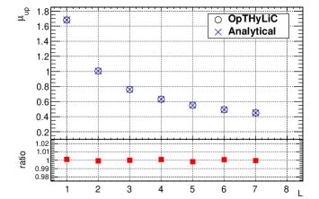
Figure 9: Upper limit $\mu_{\text{up}}$ as a function of $L$ computed with OpTHyLiC and from the analytical result (Eq. 39) for $b^{\text{nom}}=0.82\times L$, $s^{\text{nom}}=2.49\times L$ and $N^{\text{obs}}=1\times L$.

In the multiple channels case, two validations were made. In the first one, upper limits calculated with several channels were compared to upper limits calculated with a single channel in situations where the two are expected to give identical results. Such situations occur when yields in the various channels are related to each other by a simple multiplicative factor. For example, the same limits should be obtained in these two cases:

• $n$ channels each with:

  • background yield=$b^{\text{nom}}/n$

  • signal yield=$s^{\text{nom}}/n$

  • observed yield=$N^{\text{obs}}/n$

• a single channel with:

  • background yield=$b^{\text{nom}}$

  • signal yield=$s^{\text{nom}}$

  • observed yield=$N^{\text{obs}}$

It has been checked for several values of $s^{\text{nom}}$, $b^{\text{nom}}$, $N^{\text{obs}}$ and $n$ that OpTHyLiC indeed finds the same limits in both cases. In the second one, the general case where yields in the various channels can’t be related to each other by a simple multiplicative factor has been considered. It can be seen from Eq. 30 and Eq. 31 that the upper limit can be computed using the following test:

$$N_{\text{eff}}=\sum\limits_{c}N_{c}\beta_{c}\quad\text{with}\quad\beta_{c}=\ln\frac{\mu s_{c}^{\text{nom}}+b_{c}^{\text{nom}}}{b_{c}^{\text{nom}}}.$$ (40)

In the asymptotic limit, $N_{c}$ is normally distributed. Thus:

$$N_{\text{eff}}\sim{\cal N}\left(\sum\limits_{c}\beta_{c}\left(\mu s_{c}^{\text{nom}}+b_{c}^{\text{nom}}\right),\sum\limits_{c}\beta_{c}^{2}\left(\mu s_{c}^{\text{nom}}+b_{c}^{\text{nom}}\right)\right),$$ (41)

under the signal plus background hypothesis and:

$$N_{\text{eff}}\sim{\cal N}\left(\sum\limits_{c}\beta_{c}b_{c}^{\text{nom}},\sum\limits_{c}\beta_{c}^{2}b_{c}^{\text{nom}}\right),$$ (42)

under the background only hypothesis (${\cal N}\left(a,b\right)$ is the normal distribution with mean $a$ and variance $b$). $CL_{s}$ is therefore given by:

$$CL_{s}=\frac{\Phi\left(\frac{N^{\text{obs}}_{\text{eff}}\left(\mu\right)-\sum\limits_{c}\beta_{c}\left(\mu s_{c}^{\text{nom}}+b_{c}^{\text{nom}}\right)}{\sqrt{\sum\limits_{c}\beta_{c}^{2}\left(\mu s_{c}^{\text{nom}}+b_{c}^{\text{nom}}\right)}}\right)}{\Phi\left(\frac{N^{\text{obs}}_{\text{eff}}\left(\mu\right)-\sum\limits_{c}\beta_{c}b_{c}^{\text{nom}}}{\sqrt{\sum\limits_{c}\beta_{c}^{2}b_{c}^{\text{nom}}}}\right)},$$ (43)

where $\Phi$ is the cumulative distribution function of the standard normal distribution. Eq. 1 with Eq. 43 can easily be solved by dichotomy. This result has been used to validate the channel combination procedure implemented in OpTHyLiC against the asymptotic limit. Fig. 10 shows a comparison of this asymptotic result with OpTHyLiC in the three channels example defined by

• channel 1: $s^{\text{nom}}=5.18\times L$, $b^{\text{nom}}=2.22\times L$ and $N^{\text{obs}}=3\times L$

• channel 2: $s^{\text{nom}}=3.05\times L$, $b^{\text{nom}}=1.61\times L$ and $N^{\text{obs}}=4\times L$

• channel 3: $s^{\text{nom}}=4.45\times L$, $b^{\text{nom}}=2.95\times L$ and $N^{\text{obs}}=2\times L$

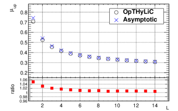
Figure 10: Upper limit $\mu_{\text{up}}$ as a function of $L$ computed with OpTHyLiC and from the asymptotic result (Eq. 43) for the three channels example defined in the text.

As can be seen from Fig. 10, OpTHyLiC converges, as expected, to the asymptotic result as the number of events increases.

6.2 Validation of calculations with statistical and systematic uncertainties

Several other studies have been performed in order to validate the treatment of statistical and systematic uncertainties in OpTHyLiC. As already explained, OpTHyLiC treats uncertainties in a Bayesian way by marginalizing the likelihood. A simple check of the marginalization procedure has been performed in the single channel case by comparing marginal distributions of the yield as computed by OpTHyLiC to analytical distributions in the case where a single background affected by a statistical uncertainty constrained with a gamma p. d. f. contributes to the expected yield. Indeed, it is known that, in this case, the marginal distribution of the yield, given by the compound of a Poisson and a gamma distribution, is negative binomial:

$$\begin{array}[]{rl}P(N=n|b^{\text{nom}},\sigma)=&\displaystyle\int_{0}^{\infty}P(N=n|b)\times f(b;b^{\text{nom}},\sigma){\rm d}b\\ &\\ =&\frac{\Gamma\left(N+\left(\frac{b^{\text{nom}}}{\sigma}\right)^{2}\right)}{N!\Gamma\left(\left(\frac{b^{\text{nom}}}{\sigma}\right)^{2}\right)}\left(\frac{b^{\text{nom}}}{b^{\text{nom}}+\sigma^{2}}\right)^{\left(b^{\text{nom}}/\sigma\right)^{2}}\left(\frac{\sigma^{2}}{b^{\text{nom}}+\sigma^{2}}\right)^{N},\\ \end{array}$$ (44)

where $N$ is the observed yield, $b$ is the background yield, $b^{\text{nom}}$ its nominal value, $\sigma$ its statistical uncertainty, $P(N=n|b)$ the Poisson distribution with parameter $b$, $f(b;b^{\text{nom}},\sigma)$ the gamma distribution for $b$ with mean $b^{\text{nom}}$ and standard deviation $\sigma$ (given by Eq. 16c) and $P(N=n|b^{\text{nom}},\sigma)$ the marginal (negative binomial) distribution of the yield $N$. Fig. 11 shows that the agreement between Eq. 44 and marginal distributions calculated by OpTHyLiC is very good. Excellent agreement has also been observed for the two other gamma definitions available in OpTHyLiC (Eq. 16a and 16b).

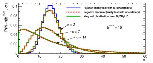
Figure 11: Marginal distribution of the yield under the background only hypothesis in the case where the background has a statistical uncertainty constrained by a gamma p. d. f. with mean $b^{\text{nom}}=15$ and three different values of standard deviation: $\sigma=2,7$ and 14.

In order to validate not only the treatment of statistical uncertainties but also that of systematic uncertainties, upper limits calculated with OpTHyLiC have been compared to upper limits calculated using a Bayesian method. It can indeed be shown that, in the single channel case, the hybrid $CL_{s}$ method implemented in OpTHyLiC is equivalent to the Bayesian method when a uniform prior on the signal strength $\mu$ is used and when the signal has no uncertainties (neither statistical nor systematic) associated to it [9]. This equivalence holds for any number of background sources, any number of statistical and systematic uncertainties associated to them and any type of correlation between systematic uncertainties across background sources. This result is used to complete the validation of the treatment of statistical uncertainties and to validate the treatment of systematic uncertainties. In order to perform this validation, an independent Bayesian software, based on RooStats, has been developed. This software implements exactly the same likelihood as OpTHyLiC and takes as input the same files, hence allowing direct comparison to OpTHyLiC. Several comparisons between OpTHyLiC and Bayesian results have been performed by changing the number of background sources and the number of systematic and statistical uncertainties. One such comparison has been performed using the configuration given in Fig. 12, with $L=1,\ldots,7$. The result is shown in Fig. 13.

+bg Bkg1 25*L 7. .syst Syst1 0.1 -0.3 .syst Syst2 0.3 -0.2 +bg Bkg2 25*L 12 .syst Syst1 0.2 -0.05 .syst Syst3 -0.06 0.15 +bg Bkg3 33.33*L 3.5 .syst Syst2 -0.1 0.3 .syst Syst3 0.15 -0.15 .syst Syst4 -0.6 0.6 +bg Bkg4 16.67*L 5 .syst Syst5 -0.3 0.25 +sig Sig 5*L +data 90*L

Figure 12: One of the examples used to validate the treatment of uncertainties in OpTHyLiC.

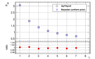
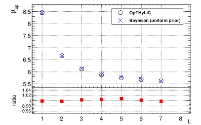
Figure 13: Upper limit $\mu_{\text{up}}$ as a function of $L$ without (left) and with (right) statistical and systematic uncertainties. It has been computed using exponential interpolation and extrapolation for systematic uncertainties and normal constraint terms for statistical uncertainty.

This example has been chosen because uncertainties are large and their effect on upper limits is very pronounced (as can be seen by comparing plots on the left and right of Fig. 13). Thus, any mis-treatment of uncertainties in OpTHyLiC should be visible. Very good agreement between OpTHyLiC and the Bayesian calculation with uniform prior is found for this example. Similar agreements are found in other cases. Rigorously, these comparisons validate only the treatment of statistical and systematic uncertaintes for backgrounds. However, signal uncertainties are treated by the same code as background uncertainties. Signal uncertainties are therefore expected to be treated properly. As will be seen below, the comparison between McLimit and OpTHyLiC gives confidence that signal uncertainties are indeed treated properly.

The last validation compares observed and expected (-2$\sigma$, -1$\sigma$, median, +1$\sigma$ and +2$\sigma$) upper limits calculated with OpTHyLiC to upper limits calculated with McLimit. McLimit, as OpTHyLiC, is a hybrid frequentist-Bayesian tool, using the interpolation/extrapolation described in Sec. 4.3.4 and normal constraints for statistical uncertainties. When configured appropriately, OpTHyLiC is therefore expected to give the same upper limits as McLimit. For this comparison, typical inputs from high energy physics analysis have been used. Fig. 14 shows a comparison of upper limits

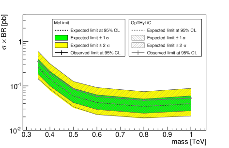
Figure 14: Comparison of observed and expected upper limits calculated with McLimit and OpTHyLiC in a realistic case (see text).

as a function of the mass of a hypothetical new particle obtained by combining three channels. Six mass points have been considered and seven background processes contribute to the yield in each channel. Signal and background processes are all affected by statistical and systematic uncertainties. For each mass, the total number of nuisance parameters is 51 (27 are associated to systematic uncertainties and 24 to statistical uncertainties). In both cases, 50 000 pseudo-experiments are used. Limits found with OpTHyLiC are in good agreement with those found with McLimit. The main difference between the two programs is the computing time. For example, on the same computer, it took 25 minutes (8 seconds) to calculate the observed limit for the 1 TeV point with McLimit (OpTHyLiC). The full plot is produced in less than 6 minutes with OpTHyLiC while it takes several hours with McLimit.

7 Conclusion

A tool computing observed and expected limits has been presented. This tool, named OpTHyLiC, is written in C++ and uses the ROOT library. It implements the hybrid frequentist-Bayesian $CL_{s}$ method for hypothesis testing. It can be used with an arbitrary number of channels and both for counting and multi-bin experiments. Statistical and systematic uncertainties are accounted for as well as correlations between systematic uncertainties. Several types of interpolation/extrapolation for systematic uncertainties and constraint terms for statistical uncertainties are provided. OpTHyLiC has been validated by comparing it to known analytical and Bayesian results and to McLimit in situations where they are expected to give identical limits. Very good agreement has been found in all cases, hence validating the software.

One of the main advantages of OpTHyLiC is its speed. Even in realistic cases with dozens of nuisance parameters and several channels and bins, the duration of limits computation remains of the order a few minutes or less.

References

References

-
[1]
OpTHyLiC webpage.
URL http://opthylic.in2p3.fr -
[2]
McLimit webpage.
URL http://www-cdf.fnal.gov/{̃}trj/mclimit/production/mclimit.html -
[3]
RooStats
webpage.
URL http://twiki.cern.ch/twiki/bin/view/RooStats - [4] A. L. Read, Presentation of search results: The technique, J. Phys. G 28 (2002) 2693–2704. doi:10.1088/0954-3899/28/10/313.
-
[5]
K. Cranmer, G. Lewis, L. Moneta, A. Shibata, W. Verkerke,
Histfactory: A tool for creating
statistical models for use with roofit and roostat.
URL http://cds.cern.ch/record/1456844/ -
[6]
ROOT webpage.
URL http://root.cern.ch - [7] M. Matsumoto, T. Nishimura, Mersenne twister: A 623-dimensionally equidistributed uniform pseudo-random number generator, ACM Trans. Model. Comput. Simul. 8 (1) (1998) 3–30. doi:10.1145/272991.272995.
-
[8]
B. Stroustrup, The C++ Programming
Language, 4th edition, Addison-Wesley, 2013.
URL http://www.stroustrup.com/4th.html - [9] E. Busato, Equivalence between hybrid and Bayesian methods for limit setting. arXiv:1404.1340.