Projected Nesterov’s Proximal-Gradient Algorithm for Sparse Signal Reconstruction with a Convex Constraint

Abstract

We develop a projected Nesterov’s proximal-gradient (PNPG) approach for sparse signal reconstruction that combines adaptive step size with Nesterov’s momentum acceleration. The objective function that we wish to minimize is the sum of a convex differentiable data-fidelity (negative log-likelihood (NLL)) term and a convex regularization term. We apply sparse signal regularization where the signal belongs to a closed convex set within the closure of the domain of the NLL; the convex-set constraint facilitates flexible NLL domains and accurate signal recovery. Signal sparsity is imposed using the $\boldsymbol{\ell}_{1}$-norm penalty on the signal’s linear transform coefficients or gradient map, respectively. The PNPG approach employs projected Nesterov’s acceleration step with restart and an inner iteration to compute the proximal mapping. We propose an adaptive step-size selection scheme to obtain a good local majorizing function of the NLL and reduce the time spent backtracking. Thanks to step-size adaptation, PNPG does not require Lipschitz continuity of the gradient of the NLL. We present an integrated derivation of the momentum acceleration and its $\boldsymbol{\mathcal{O}(k^{-2})}$ convergence-rate and iterate convergence proofs, which account for adaptive step-size selection, inexactness of the iterative proximal mapping, and the convex-set constraint. The tuning of PNPG is largely application-independent. Tomographic and compressed-sensing reconstruction experiments with Poisson generalized linear and Gaussian linear measurement models demonstrate the performance of the proposed approach.

I Introduction

Most natural signals are well described by only a few significant coefficients in an appropriate transform domain, with the number of significant coefficients much smaller than the signal size. Therefore, for a vector ${\boldsymbol{x}}\in\mathamsbb{R}^{p\times 1}$ that represents the signal and an appropriate sparsifying transform $\boldsymbol{\psi}(\cdot)\mathrel{\mathop{\mathchar 58\relax}}\mathamsbb{R}^{p}\mapsto\mathamsbb{R}^{p^{\prime}}$, $\boldsymbol{\psi}({\boldsymbol{x}})$ is a signal transform-coefficient vector with most elements having negligible magnitudes. The idea behind compressed sensing [1] is to sense the significant components of $\boldsymbol{\psi}({\boldsymbol{x}})$ using a small number of measurements. Define the noiseless measurement vector $\boldsymbol{\phi}({\boldsymbol{x}})$, where $\boldsymbol{\phi}(\cdot)\mathrel{\mathop{\mathchar 58\relax}}\mathamsbb{R}^{p}\mapsto\mathamsbb{R}^{N}$ and $N\leq p$. Most effort in compressed sensing has focused on the linear sparsifying transform and noiseless measurement models with

$$\boldsymbol{\psi}({\boldsymbol{x}})=\Psi^{T}{\boldsymbol{x}}$$ (1a)

$$\boldsymbol{\phi}({\boldsymbol{x}})=\Phi{\boldsymbol{x}}$$ (1b)

where $\Psi\in\mathamsbb{R}^{p\times p^{\prime}}$ and $\Phi\in\mathamsbb{R}^{N\times p}$ are known sparsifying dictionary and sensing matrices. Here, we consider signals ${\boldsymbol{x}}$ that belong to a closed convex set $C$ in addition to their sparsity in the transform domain. The nonnegative signal scenario with

$$C=\mathamsbb{R}_{+}^{p}$$ (2)

is of significant practical interest and applicable to X-ray computed tomography (CT), single photon emission computed tomography (SPECT), positron emission tomography (PET), and magnetic resonance imaging (MRI), where the pixel values correspond to inherently nonnegative density or concentration maps [2]. [3] consider such a nonnegative sparse signal model and develop in [3] and [4] a convex-relaxation sparse Poisson-intensity reconstruction algorithm (SPIRAL) and a linearly constrained gradient projection method for Poisson and Gaussian linear measurements, respectively. In addition to signal nonnegativity, other convex-set constraints have been considered in the literature, such as prescribed value in the Fourier domain; box, geometric, and total-energy constraints; and intersections of these sets [5, 6].

We adopt the analysis regularization framework and minimize

$$f({\boldsymbol{x}})=\mathcal{L}({\boldsymbol{x}})+ur({\boldsymbol{x}})$$ (3a)

with respect to the signal $${\boldsymbol{x}} \mathcal{L}({\boldsymbol{x}}) u>0 r({\boldsymbol{x}})$$, where is a convex differentiable data-fidelity (negative log-likelihood (NLL)) term, is a scalar tuning constant that quantifies the weight of the convex regularization term that imposes signal sparsity and the convex-set constraint:

$$r({\boldsymbol{x}})=\lVert\boldsymbol{\psi}({\boldsymbol{x}})\rVert_{1}+\mathamsbb{I}_{C}({\boldsymbol{x}})$$ (3b)

and $\mathamsbb{I}_{C}({\boldsymbol{a}})\triangleq\begin{cases}0,&{\boldsymbol{a}}\in C\\ +\infty,&\text{otherwise}\end{cases}$ is the indicator function. Common choices for the signal sparsifying transform are the linear map in (1a), isotropic gradient map

$$\left[\boldsymbol{\psi}({\boldsymbol{x}})\right]_{i=1}^{p^{\prime}}\triangleq\sqrt{\sum_{j\in\mathcal{N}_{i}}(x_{i}-x_{j})^{2}}$$ (4)

and their combinations; here, $\mathcal{N}_{i}$ is the index set of neighbors of $x_{i}$ in an appropriate (e.g., 2D) arrangement. Summing (4) over $i$ leads to the isotropic total-variation (TV) penalty [7, 3, 8]; in the 2D case, anisotropic TV penalty is slightly different and easy to accommodate as well. Assume

$$C\subseteq\operatorname{cl}(\operatorname{dom}\mathcal{L}({\boldsymbol{x}}))$$ (5)

which ensures that $\mathcal{L}({\boldsymbol{x}})$ is computable for all ${\boldsymbol{x}}\in\operatorname{int}C$ and closure ensures that points in $\operatorname{dom}\mathcal{L}$ but close to its open boundary, if there is any, will not be excluded upon projecting onto the closed set $C$. If $C\setminus\operatorname{dom}\mathcal{L}=C\cap\bigl{[}\operatorname{cl}(\operatorname{dom}\mathcal{L}({\boldsymbol{x}}))\setminus\operatorname{dom}\mathcal{L}\bigr{]}$ is not empty, then $\mathcal{L}({\boldsymbol{x}})$ is not computable in it, which needs special attention; see Section III.

Define the proximal operator for a function $r({\boldsymbol{x}})$ scaled by $\lambda$:

$$\operatorname{prox}_{\lambda r}{\boldsymbol{a}}=\arg\min_{{\boldsymbol{x}}}\tfrac{1}{2}\lVert{\boldsymbol{x}}-{\boldsymbol{a}}\rVert_{2}^{2}+\lambda r({\boldsymbol{x}}).$$ (6)

References [9, 10, 11] view (3a) as a sum of three terms, $\mathcal{L}({\boldsymbol{x}})$, $\lVert\boldsymbol{\psi}({\boldsymbol{x}})\rVert_{1}$, and $\mathamsbb{I}_{C}({\boldsymbol{x}})$, and minimize it by splitting schemes, such as forward-backward, Douglas-Rachford, and primal-dual. A potential benefit of splitting schemes is that they apply proximal operations on individual summands rather than on their combination, which is useful if all individual proximal operators are easy to compute. However, [9] requires the proximal operator of $\mathcal{L}({\boldsymbol{x}})$, which is difficult in general and needs an inner iteration. Both [9] and generalized forward-backward (GFB) splitting [10] require inner iterations for solving $\operatorname{prox}_{\lambda\lVert\Psi^{T}\cdot\rVert_{1}}{\boldsymbol{a}}$ (see (1a) and (6)) in the general case where the sparsifying matrix $\Psi$ is not orthogonal. The elegant primal-dual splitting (PDS) method in [11, 12] does not require inner iterations. The convergence rate of both GFB and PDS methods can be upper-bounded by $C/k$ where $k$ is the number of iterations and the constant $C$ is determined by values of the tuning proximal and relaxation constants [13, 14].

In this paper, we develop a projected Nesterov’s proximal-gradient (PNPG) method whose momentum acceleration accommodates (increasing) adaptive step size selection (see also [7, 15, 16]) and convex-set constraint on the signal ${\boldsymbol{x}}$. PNPG needs an inner iteration to compute the proximal operator with respect to $r({\boldsymbol{x}})$, which implies inexact proximal operation. We account for this inexactness and establish ${\mathcal{O}(k^{-2})}$ convergence rate of the PNPG method as well as convergence of its iterates; the obtained convergence conditions motivate our selection of convergence criteria for proximal-mapping iterations. We modify the original Nesterov’s acceleration [17, 18] so that we can establish these convergence results when the step size is adaptive and adjusts to the local curvature of the NLL. Thanks to the step-size adaptation, PNPG does not require Lipschitz continuity of the gradient of the NLL and applies to the Poisson compressed-sensing scenario described in Section II-A. Our integration of the adaptive step size and convex-set constraint extends the application of the Nesterov-type acceleration to more general measurement models than those used previously. Furthermore, a convex-set constraint can bring significant improvement to signal reconstructions compared with imposing signal sparsity only, as illustrated in Section V-B. See Section IV-A for discussion of other ${\mathcal{O}(k^{-2})}$ acceleration approaches: Auslender-Teboulle (AT) [19, 20] and [21] [21]. Proximal Quasi-Newton type methods with problem-specific diagonal Hessian approximations have been considered in [21, 22]; [22] applies step-size adaptation and accounts for inaccurate proximal operator, but does not employ acceleration or provide fast convergence-rate guarantees.

PNPG code is easy to maintain: for example, the proximal-mapping computation can be easily replaced as a module by the latest state-of-the-art solver. Furthermore, PNPG requires minimal application-independent tuning; indeed, we use the same set of tuning parameters in two different application examples. This is in contrast with the existing splitting methods, which require problem-dependent (NLL-dependent) design and tuning.

We introduce the notation: $\boldsymbol{0}$, $\boldsymbol{1}$, $I$, denote the vectors of zeros and ones and identity matrix, respectively; “$\succeq$” is the elementwise version of “$\geq$”. For a vector $\boldsymbol{a}=(a_{i})_{i=1}^{N}\in\mathamsbb{R}^{N\times 1}$, define the projection and soft-thresholding operators:

$$P_{C}({\boldsymbol{a}}) = \arg\min_{{\boldsymbol{x}}\in C}\lVert{\boldsymbol{x}}-{\boldsymbol{a}}\rVert_{2}^{2}$$ (7a)

$$\left[\operatorname{\mathcal{T}}_{\lambda}({\boldsymbol{a}})\right]_{i} = \operatorname{sgn}(a_{i})\max\left({\lvert a_{i}\rvert-\lambda,0}\right)$$ (7b)

and the elementwise logarithm and exponential functions $$[\ln_{\circ}{\boldsymbol{a}}]_{i}=\ln a_{i} [\exp_{\circ}{\boldsymbol{a}}]_{i}=\exp a_{i} \mathamsbb{R}_{+}^{N} \ell_{1} \|{\boldsymbol{x}}\|_{1}$$ and . The projection onto and the proximal operator (6) for the -norm can be computed in closed form:

$$\bigl{[}P_{\mathamsbb{R}_{+}^{N}}({\boldsymbol{a}})\bigr{]}_{i}=\max(a_{i},0), \operatorname{prox}_{\lambda\lVert\cdot\rVert_{1}}{\boldsymbol{a}}=\operatorname{\mathcal{T}}_{\lambda}({\boldsymbol{a}}).$$ (7c)

Define the $\varepsilon$-subgradient [23, Sec. 23]:

$$\partial_{\varepsilon}r({\boldsymbol{x}}) \triangleq \bigl{\{}\boldsymbol{g}\in\mathamsbb{R}^{p}\mid r(\boldsymbol{z})\geq r({\boldsymbol{x}})+(\boldsymbol{z}-{\boldsymbol{x}})^{T}\boldsymbol{g}-\varepsilon,\forall\boldsymbol{z}\in\mathamsbb{R}^{p}\bigr{\}}$$

and an inexact proximal operator:

Definition 1

We say that ${\boldsymbol{x}}$ is an approximation of $\operatorname{prox}_{ur}\!\left({{\boldsymbol{a}}}\right)$ with $\varepsilon$-precision [24], denoted

$${\boldsymbol{x}}\approxeq_{\varepsilon}\operatorname{prox}_{ur}{\boldsymbol{a}}$$ (9a)

if

$$\frac{{\boldsymbol{a}}-{\boldsymbol{x}}}{u}\in\partial_{\frac{\varepsilon^{2}}{2u}}r({\boldsymbol{x}}).$$ (9b)

Note that (9a) implies

$$\lVert{\boldsymbol{x}}-\operatorname{prox}_{ur}{\boldsymbol{a}}\rVert_{2}^{2}\leq\varepsilon^{2}.$$ (10)

We introduce representative NLL functions in Section II, describe the proposed PNPG reconstruction algorithm in Section III, establish its convergence properties (Section IV), present numerical examples (Section V), and make concluding remarks (Section VI).

II Probabilistic Measurement Models

For numerical stability, we normalize the likelihood function so that the corresponding NLL $\mathcal{L}({\boldsymbol{x}})$ is lower-bounded by zero. For NLLs that correspond to discrete generalized linear models (GLMs), this normalization corresponds to the generalized Kullback-Leibler divergence form of the NLL and is also closely related to the Bregman divergence [25].

II-A Poisson Generalized Linear Model

GLMs with Poisson observations are often adopted in astronomic, optical, hyperspectral, and tomographic imaging [26, 2, 27, 28] and used to model event counts, e.g., numbers of particles hitting a detector. Assume that the measurements $\boldsymbol{y}=(y_{n})_{n=1}^{N}\in\mathamsbb{N}_{0}^{N}$ are independent Poisson-distributed with means $[\boldsymbol{\phi}({\boldsymbol{x}})]_{n}$.

Upon ignoring constant terms and normalization, we obtain the generalized Kullback-Leibler divergence form [29] of the NLL

$$\mathcal{L}({\boldsymbol{x}})=\boldsymbol{1}^{T}[\boldsymbol{\phi}({\boldsymbol{x}})-\boldsymbol{y}]+\sum_{n,y_{n}\neq 0}y_{n}\ln\frac{y_{n}}{[\boldsymbol{\phi}({\boldsymbol{x}})]_{n}}.$$ (11a)

The NLL $$\mathcal{L}({\boldsymbol{x}})\mathrel{\mathop{\mathchar 58\relax}}\mathamsbb{R}^{p}\mapsto\mathamsbb{R}_{+} {\boldsymbol{x}} \Phi{\boldsymbol{x}} \boldsymbol{\phi}({\boldsymbol{x}}) \boldsymbol{y} \boldsymbol{g}(\cdot)\mathrel{\mathop{\mathchar 58\relax}}\mathamsbb{R}^{N}\mapsto\mathamsbb{R}^{N}$$ is a convex function of the signal . Here, the relationship between the linear predictor and the expected value of the measurements is summarized by the link function [30]:

$$\operatorname{E}(\boldsymbol{y})=\boldsymbol{\phi}({\boldsymbol{x}})=\boldsymbol{g}^{-1}(\Phi{\boldsymbol{x}}).$$ (11b)

Note that $\operatorname{cl}(\operatorname{dom}\mathcal{L})=\{{\boldsymbol{x}}\in\mathamsbb{R}^{p}\mid\boldsymbol{\phi}({\boldsymbol{x}})\succeq\boldsymbol{0}\}$.

Two typical link functions in the Poisson GLM are log and identity, described in the following:

II-A1 Identity link

The identity link function with

$$\boldsymbol{g}(\boldsymbol{\mu})=\boldsymbol{\mu}-{\boldsymbol{b}}, \,\boldsymbol{\phi}({\boldsymbol{x}})=\Phi{\boldsymbol{x}}+{\boldsymbol{b}}$$ (12)

is used for modeling the photon count in optical imaging [28] and radiation activity in emission tomography [2, Ch. 9.2], as well as for astronomical image deconvolution [27, Sec. 3.5.4]. Here, $\Phi=\in\mathamsbb{R}_{+}^{N\times p}$ and ${\boldsymbol{b}}\in\mathamsbb{R}_{+}^{N\times 1}$ are the known sensing matrix and intercept term, respectively; the intercept ${\boldsymbol{b}}$ models background radiation and scattering determined, e.g., by calibration before the measurements $\boldsymbol{y}$ have been collected. The nonnegative set $C$ in (2) satisfies (5), where we have used the fact that the elements of $\Phi$ are nonnegative. If ${\boldsymbol{b}}$ has zero components, $C\setminus\operatorname{dom}\mathcal{L}$ is not empty and the NLL does not have a Lipschitz-continuous gradient.

Setting ${\boldsymbol{b}}=\boldsymbol{0}$ leads to the identity link without intercept used, e.g., in [28, 27, 3].

II-A2 Log link

The log-link function

$$\boldsymbol{g}(\boldsymbol{\mu})=-{\ln_{\circ}({\boldsymbol{\mu}}/{\mathcal{I}_{0}})}, \boldsymbol{\phi}({\boldsymbol{x}})=\mathcal{I}_{0}\exp_{\circ}(-\Phi{\boldsymbol{x}})$$ (13)

has been used to account for the exponential attenuation of particles (e.g., in tomographic imaging), where $\mathcal{I}_{0}$ is the incident energy before attenuation. The intercept term $\mathcal{I}_{0}$ is often assumed known [31, Sec. 8.10]. The Poisson GLM with log link function is referred to as the log-linear model in [30, Ch. 6], which treats known and unknown $\mathcal{I}_{0}$ as the same model.

Log link with unknown intercept. For unknown $\mathcal{I}_{0}$, (11a) does not hold because the underlying NLL is a function of both ${\boldsymbol{x}}$ and $\mathcal{I}_{0}$. Substituting (13) into the NLL function, concentrating it with respect to $\mathcal{I}_{0}$, and ignoring constant terms yields the following convex concentrated (profile) NLL:

$$\mathcal{L}_{\textup{c}}({\boldsymbol{x}})=\boldsymbol{1}^{T}\boldsymbol{y}\ln\bigl{[}\boldsymbol{1}^{T}\exp_{\circ}(-\Phi{\boldsymbol{x}})\bigr{]}+\boldsymbol{y}^{T}\Phi{\boldsymbol{x}}$$ (14)

see [16, App. LABEL:report-app:derconcentratednllpoisson], where we also derive the Hessian of (14). Note that $\operatorname{dom}\mathcal{L}_{\textup{c}}({\boldsymbol{x}})=\mathamsbb{R}^{p}$; hence, any closed convex $C$ satisfies (5).

II-B Linear Model with Gaussian Noise

Linear measurement model (1b) with zero-mean additive white Gaussian noise (AWGN) leads to the following scaled NLL:

$$\mathcal{L}({\boldsymbol{x}})=\frac{1}{2}\|\boldsymbol{y}-\Phi{\boldsymbol{x}}\|_{2}^{2}$$ (15)

where $\boldsymbol{y}\in\mathamsbb{R}^{N}$ is the measurement vector and constant terms (not functions of ${\boldsymbol{x}}$) have been ignored. This NLL belongs to the Gaussian GLM with identity link without intercept: $\boldsymbol{g}(\boldsymbol{\mu})=\boldsymbol{\mu}$. Here, $\operatorname{dom}\mathcal{L}({\boldsymbol{x}})=\mathamsbb{R}^{p}$, any closed convex $C$ satisfies (5), and the set $C\setminus\operatorname{dom}\mathcal{L}$ is empty.

Minimization of the objective function (3a) with penalty (3b) and Gaussian NLL (15) can be thought of as an analysis basis pursuit denoising (BPDN) problem with a convex signal constraint; see also [16, 15] which use the nonnegative $C$ in (2). A synthesis BPDN problem with a convex signal constraint was considered in [32].

III Reconstruction Algorithm

We propose a PNPG approach for minimizing (3a) that combines convex-set projection with Nesterov acceleration [17, 18] and applies adaptive step size to adapt to the local curvature of the NLL and restart to ensure monotonicity of the resulting iteration. The pseudo code in Algorithm 1 summarizes our PNPG method.

Input: ${\boldsymbol{x}}^{(0)}$, $u$, $\gamma$, $b$, $\mathbb{n}$, $\mathbb{m}$, $\xi$, $\eta$, and threshold $\epsilon$

Output: $\arg\min_{\boldsymbol{x}}f({\boldsymbol{x}})$

Initialization: ${\boldsymbol{x}}^{(-1)}\leftarrow\boldsymbol{0}$, $i\leftarrow 0$, $\kappa\leftarrow 0$, $\beta^{(1)}$ by the BB method

repeat

       $i\leftarrow i+1$ and $\kappa\leftarrow\kappa+1$

       while true do // backtracking search

             evaluate (17a) to (17d)

             if ${\overline{{\boldsymbol{x}}}}^{(i)}\notin\operatorname{dom}\mathcal{L}$ then // domain restart

                   $\theta^{(i-1)}\leftarrow 1$ and continue

                  

            solve the proximal-mapping step (17e)

             if majorization condition (18) holds then

                   break

                  

            else

                   if $\beta^{(i)}>\beta^{(i-1)}$ then // increase $\mathbb{n}$

                         $\mathbb{n}\leftarrow\mathbb{n}+\mathbb{m}$

                  $\beta^{(i)}\leftarrow\xi\beta^{(i)}$ and $\kappa\leftarrow 0$

                  

            

      if $i>1$ and $f\bigl{(}{\boldsymbol{x}}^{(i)}\bigr{)}>f\bigl{(}{\boldsymbol{x}}^{(i-1)}\bigr{)}$ then // restart

             $\theta^{(i-1)}\leftarrow 1$, $i\leftarrow i-1$, and continue

      if convergence condition (29) holds with threshold $\epsilon$  then

             declare convergence

      if $\kappa\geq\mathbb{n}$ then // adapt step size

             $\kappa\leftarrow 0$ and $\beta^{(i+1)}\leftarrow{\beta^{(i)}}/{\xi}$

      else

             $\beta^{(i+1)}\leftarrow\beta^{(i)}$

      

until  convergence declared or maximum number of iterations exceeded

Algorithm 1 PNPG iteration

Define the quadratic approximation of the NLL $\mathcal{L}({\boldsymbol{x}})$:

$$Q_{\beta}({\boldsymbol{x}}\mid{\overline{{\boldsymbol{x}}}})=\mathcal{L}({\overline{{\boldsymbol{x}}}})+({\boldsymbol{x}}-{\overline{{\boldsymbol{x}}}})^{T}\nabla\mathcal{L}({\overline{{\boldsymbol{x}}}})+\frac{1}{2\beta}\lVert{\boldsymbol{x}}-{\overline{{\boldsymbol{x}}}}\rVert_{2}^{2}$$ (16)

with $\beta$ chosen so that (16) majorizes $\mathcal{L}({\boldsymbol{x}})$ in the neighborhood of ${\boldsymbol{x}}={\overline{{\boldsymbol{x}}}}$. Iteration $i$ of the PNPG method proceeds as follows:

$$B^{(i)} = {\beta^{(i-1)}}/{\beta^{(i)}}$$ (17a)

$$\theta^{(i)} = \begin{cases}1,&i\leq 1\\ \frac{1}{\gamma}+\sqrt{{b}+B^{(i)}(\theta^{(i-1)})^{2}},&i>1\end{cases}$$ (17b)

$$\Theta^{(i)} = \bigl{(}\theta^{(i-1)}-1\bigr{)}/{\theta^{(i)}}$$ (17c)

$${\overline{{\boldsymbol{x}}}}^{(i)} = P_{C}\Bigl{(}{\boldsymbol{x}}^{(i-1)}+\Theta^{(i)}\bigl{(}{\boldsymbol{x}}^{(i-1)}-{\boldsymbol{x}}^{(i-2)}\bigr{)}\Bigr{)}$$ (17d)

$${\boldsymbol{x}}^{(i)} = \operatorname{prox}_{\beta^{(i)}ur}\!\bigl{(}{\overline{{\boldsymbol{x}}}}^{(i)}-\beta^{(i)}\nabla\mathcal{L}({\overline{{\boldsymbol{x}}}}^{(i)})\bigr{)}$$ (17e)

where $\beta^{(i)}>0$ is an adaptive step size chosen to satisfy the majorization condition

$$\mathcal{L}({\boldsymbol{x}}^{(i)}) \leq Q_{\beta^{(i)}}({\boldsymbol{x}}^{(i)}\mid{{\overline{{\boldsymbol{x}}}}}^{(i)})$$ (18)

using a simple adaptation scheme that aims at keeping $\beta^{(i)}$ as large as possible, described in Section III-B; see also Algorithm 1. Here,

$$\gamma\geq 2, b\in[0,1/4]$$ (19)

in (17b) are momentum tuning constants and $\gamma$ controls the rate of increase of the extrapolation term $\theta^{(i)}$. We will denote $\theta^{(i)}$ as $\theta_{\gamma,b}^{(i)}$ when we wish to emphasize its dependence on $\gamma$ and $b$.

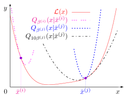
Figure 1: Local and global majorizing functions.

Note that $Q_{\beta}({\boldsymbol{x}}\mid{\overline{{\boldsymbol{x}}}})$ is a local majorizer of $\mathcal{L}({\boldsymbol{x}})$ in the neighborhood of ${\overline{{\boldsymbol{x}}}}$: unlike most existing work, we require (18) to hold only for ${\boldsymbol{x}}^{(i)}$, i.e., $\mathcal{L}({\boldsymbol{x}})\nleq Q_{\beta^{(i)}}({\boldsymbol{x}}\mid{{\overline{{\boldsymbol{x}}}}}^{(i)})$ in general, which violates the conventional textbook definitions of majorizing functions that require global, rather than local, majorization; see also Fig. 1 and [33, Sec. 5.8 and Fig. 5.10]. By relaxing the global majorization requirement, we aim to obtain a local majorizer such as $Q_{10\beta^{(j)}}$, which approximates the NLL function better in the neighborhood of $\bar{{\boldsymbol{x}}}^{(j)}$ than the global majorizer and also provides the same monotonicity guarantees as the global majorizer as long as the majorization condition holds at the new iterate to which we move next.

For $\boldsymbol{\psi}(\cdot)$ in (1a) and (4), we compute the proximal mapping (17e) using the alternating direction method of multipliers (ADMM) in Section III-C and TV-based denoising method in [8], respectively. Because of its iterative nature, (17e) is inexact; this inexactness can be modeled as

$${\boldsymbol{x}}^{(i)}\approxeq_{\varepsilon^{(i)}}\operatorname{prox}_{\beta^{(i)}ur}\!\bigl{(}{\overline{{\boldsymbol{x}}}}^{(i)}-\beta^{(i)}\nabla\mathcal{L}({\overline{{\boldsymbol{x}}}}^{(i)})\bigr{)}$$ (20)

where $\varepsilon^{(i)}$ quantifies the precision of the proximal-gradient (PG) step in Iteration $i$.

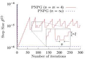
(a) Poisson model with identity link.

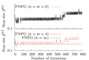
(b) Gaussian linear model.

Figure 2: Step sizes $\beta^{(i)}$ as functions of the number of iterations for Poisson and Gaussian linear models.

The acceleration step (17d) extrapolates the two latest iteration points in the direction of their difference ${\boldsymbol{x}}^{(i)}-{\boldsymbol{x}}^{(i-1)}$, followed by the projection onto the convex set $C$. For nonnegative $C$ in (2), this projection has closed form, see (7c). If $C$ is an intersection of convex sets with simple individual projection operator for each, we can apply projections onto convex sets (POCS) [5].

If we remove the signal-sparsity penalty term by setting $\boldsymbol{\psi}(\cdot)=\boldsymbol{0}$, the proximal mapping in (17e) reduces to the projection onto $C$ and the iteration (17) becomes a projected Nesterov’s projected gradient method: an approach to accelerate projected gradient methods that ensures that the gradient of the NLL is computable at the extrapolated value ${\overline{{\boldsymbol{x}}}}^{(i)}$. When projection onto $C$ is simple, a suboptimal ad hoc approach that avoids inner proximal-mapping iteration can be constructed as follows: replace the first summand in (3b) with a differentiable approximation and then append the resulting approximate term to the NLL term, thus leaving $r({\boldsymbol{x}})$ with the indicator function only, which leads to the projected Nesterov’s projected gradient method. A similar approach has been used in [21] in its Poisson image deblurring numerical example.

If we remove the convex-set constraint by setting $C=\mathamsbb{R}^{p}$, iteration (17a)–(17e) reduces to the Nesterov’s proximal-gradient iteration with adaptive step size that imposes signal sparsity only in the analysis form (termed NPG${}_{\text{S}}$); see also Section V-B for an illustrative comparison of NPG${}_{\text{S}}$ and PNPG.

We now extend [18, Lemma 2.3] to the inexact proximal operation:

Lemma 1

Assume convex and differentiable NLL $\mathcal{L}({\boldsymbol{x}})$ and convex $r({\boldsymbol{x}})$ and consider an inexact PG step (20) with step size $\beta^{(i)}$ that satisfies the majorization condition (18). Then,

$$f({\boldsymbol{x}})-f({\boldsymbol{x}}^{(i)}) \geq \frac{1}{2\beta^{(i)}}\bigl{[}\lVert{\boldsymbol{x}}^{(i)}-{\boldsymbol{x}}\rVert_{2}^{2}-\lVert{\overline{{\boldsymbol{x}}}}^{(i)}-{\boldsymbol{x}}\rVert_{2}^{2}-(\varepsilon^{(i)})^{2}\bigr{]}$$

for all $i\geq 1$ and any ${\boldsymbol{x}}\in\mathamsbb{R}^{p}$.

Proof:

See Appendix A. ∎

Lemma 1 is general and algorithm-independent because ${\overline{{\boldsymbol{x}}}}^{(i)}$ can be any value in $\operatorname{dom}\mathcal{L}$, the regularization term $r({\boldsymbol{x}})$ can be any convex function, and we have used only the fact that step size $\beta^{(i)}$ satisfies the majorization condition (18), rather than specific details of the step-size selection. We will use this result to establish the monotonicity property in Remark 1 and as the starting point for deriving and analyzing our accelerated PG scheme.

III-A Restart and Monotonicity

If $f({\boldsymbol{x}}^{(i)})>f({\boldsymbol{x}}^{(i-1)})$ or ${\overline{{\boldsymbol{x}}}}^{(i)}\in C\setminus\operatorname{dom}\mathcal{L}$, set

$$\theta^{(i-1)}=1 (restart)$$ (22)

and refer to this action as function restart [34] or domain restart respectively; see Algorithm 1. The goal of function and domain restarts is to ensure that the PNPG iteration is monotonic and ${\overline{{\boldsymbol{x}}}}^{(i)}$ remains within $\operatorname{dom}f$ as long as the projected initial value is within $\operatorname{dom}f$: $f\bigl{(}P_{C}({\boldsymbol{x}}^{(0)})\bigr{)}<+\infty$.

The majorization condition (18) ensures that the iterate ${\boldsymbol{x}}^{(i)}$ attains lower (or equal) objective function than the intermediate signal $\overline{{\boldsymbol{x}}}^{(i)}$ (see Lemma 1 with ${\overline{{\boldsymbol{x}}}}^{(i)}$ in place of ${\boldsymbol{x}}$)

$$f({\boldsymbol{x}}^{(i)})\leq f(\overline{{\boldsymbol{x}}}^{(i)})-\frac{1}{2\beta^{(i)}}\bigl{[}\lVert{\boldsymbol{x}}^{(i)}-\overline{{\boldsymbol{x}}}^{(i)}\rVert^{2}_{2}-(\varepsilon^{(i)})^{2}\bigr{]}$$ (23)

provided that proximal-mapping approximation error term $(\varepsilon^{(i)})^{2}$ is sufficiently small. However, (23) does not guarantee monotonicity of the PNPG iteration: we apply the function restart to restore the monotonicity and improve convergence of the PNPG iteration; see Algorithm 1.

Define the local variation of signal iterates

$$\delta^{(i)}\triangleq\lVert{\boldsymbol{x}}^{(i)}-{\boldsymbol{x}}^{(i-1)}\rVert_{2}^{2}.$$ (24)

Remark 1 (Monotonicity)

The PNPG iteration with restart and inexact PG steps (20) is non-increasing:

$$f({\boldsymbol{x}}^{(i)})\leq f({\boldsymbol{x}}^{(i-1)})$$ (25a)

for all $$i$$ if the inexact PG steps are sufficiently accurate and satisfy

$$\varepsilon^{(i)}\leq\sqrt{\delta^{(i)}}.$$ (25b)

Proof:

If there is no restart in Iteration $i$, the objective function has not increased. If there is a restart, $\theta^{(i-1)}=1$ and (17d) simplifies to ${\overline{{\boldsymbol{x}}}}^{(i)}=P_{C}\bigl{(}{\boldsymbol{x}}^{(i-1)}\bigr{)}={\boldsymbol{x}}^{(i-1)}$, and monotonicity follows upon substituting ${\overline{{\boldsymbol{x}}}}^{(i)}={\boldsymbol{x}}^{(i-1)}$ into (23).∎

To establish the monotonicity in Remark 1, we only need the step size $\beta^{(i)}$ to satisfy the majorization condition (18). Small $\varepsilon^{(i)}$ can be achieved by selecting the inner-iteration convergence criteria appropriately; see Section III-D.

The condition (25b) motivates us to incorporate $\delta^{(i-1)}$ into the convergence criteria for proximal-step computation, see Section III-D.

III-B Adaptive Step Size

Now, we present an adaptive scheme for selecting $\beta^{(i)}$:

1. • if there have been no step-size backtracking events or increase attempts for $\mathbb{n}$ consecutive iterations ($i-\mathbb{n}$ to $i-1$), start with a larger step size

     $$\overline{\beta}^{(i)}={\beta^{(i-1)}}/{\xi} (increaseattempt)$$ (26a)

     where

     $$\xi\in(0,1)$$ (26b)

     is a step-size adaptation parameter;

   • otherwise start with

     $$\overline{\beta}^{(i)}=\beta^{(i-1)};$$ (26c)

2. (backtracking search) select

   $$\beta^{(i)}=\xi^{t_{i}}\overline{\beta}^{(i)}$$ (26d)

   where $t_{i}\geq 0$ is the smallest integer such that (26d) satisfies the majorization condition (18); backtracking event corresponds to $t_{i}>0$.

3. if $\max(\beta^{(i)},\beta^{(i-1)})<\overline{\beta}^{(i)}$, increase $\mathbb{n}$ by a nonnegative integer $\mathbb{m}$:

   $$\mathbb{n}\leftarrow\mathbb{n}+\mathbb{m}.$$ (26e)

We select the initial step size $\overline{\beta}^{(1)}$ using the Barzilai-Borwein (BB) method [35].

If there has been an attempt to change the step size in any of the previous $\mathbb{n}$ consecutive iterations, we start the backtracking search ii) with the step size from the latest completed iteration. Consequently, the step size will be approximately piecewise-constant as a function of the iteration index $i$; see Fig. 2, which shows the evolutions of the adaptive step size $\beta^{(i)}$ for measurements following the Poisson generalized linear and Gaussian linear models corresponding to Figs. 5(a) and 8(b); see Sections V-A and V-B for details of the two simulation scenarios. Here, $\mathbb{n}$ controls the size of the neighborhood around ${\overline{{\boldsymbol{x}}}}^{(i)}$ over which $Q_{\beta^{(i)}}\bigl{(}{\boldsymbol{x}}\mid{{\overline{{\boldsymbol{x}}}}}^{(i)}\bigr{)}$ majorizes $\mathcal{L}({\boldsymbol{x}})$ and also the time spent backtracking: larger $\mathbb{n}$ yields a larger neighborhood and leads to less backtracking. To reduce sensitivity to the choice of the tuning constant $\mathbb{n}$, we adapt it by increasing its value by $\mathbb{m}$ if there is a failed attempt to increase the step size in Iteration $i$, i.e., $\overline{\beta}^{(i)}>\beta^{(i-1)}$ and $\beta^{(i)}<\overline{\beta}^{(i)}$.

The adaptive step-size strategy keeps $\beta^{(i)}$ as large as possible subject to (18), which is important not only because the signal iterate may reach regions of $\mathcal{L}({\boldsymbol{x}})$ with different local Lipschitz constants, but also due to the varying curvature of $\mathcal{L}({\boldsymbol{x}})$ in different updating direction. For example, a (backtracking-only) PG-type algorithm with non-adaptive step size would fail or converge very slowly if the local Lipschitz constant of $\nabla\mathcal{L}({\boldsymbol{x}})$ decreases as the algorithm iterates because the step size will not be able to adjust and track this decrease; see also Section V where the benefits of step-size adaptation are demonstrated by numerical examples.

Setting $\mathbb{n}=+\infty$ corresponds to step-size backtracking only, which aims at finding $\beta^{(i)}/\xi$ upper bounding the inverse of the (global) Lipschitz constant of $\nabla\mathcal{L}({\boldsymbol{x}})$. A step-size adaptation scheme with $\mathbb{n}=\mathbb{m}=0$ initializes the step-size search aggressively, with an increase attempt (26a) in each iteration.

III-C ADMM Proximal Mapping for $\ell_{1}$-Norm Penalty with Linear Transform Coefficients

We present an ADMM scheme for computing the proximal operator (6) with $\boldsymbol{\psi}({\boldsymbol{x}})$ in (1a):

$$\bar{{\boldsymbol{a}}}^{(i)} = \bigl{(}I+\rho\Psi\Psi^{T}\bigr{)}^{-1}\bigl{[}{\boldsymbol{a}}+\rho\Psi(\boldsymbol{s}^{(j-1)}+\boldsymbol{\upsilon}^{(j-1)})\bigr{]}$$ (27a)

$${\boldsymbol{\alpha}}^{(j)} = \arg\min_{{\boldsymbol{\alpha}}\in C}\bigl{\|}{\boldsymbol{\alpha}}-\bar{{\boldsymbol{a}}}^{(i)}\bigr{\|}_{I+\rho\Psi\Psi^{T}}^{2}$$ (27b)

$$\boldsymbol{s}^{(j)} = \mathcal{T}_{{\lambda}/{\rho}}\bigl{(}\Psi^{T}{\boldsymbol{\alpha}}^{(j)}-\boldsymbol{\upsilon}^{(j-1)}\bigr{)}$$ (27c)

$$\boldsymbol{\upsilon}^{(j)} = \boldsymbol{\upsilon}^{(j-1)}+\boldsymbol{s}^{(j)}-\Psi^{T}{\boldsymbol{\alpha}}^{(j)}$$ (27d)

where $j$ is the ADMM iteration index and $\rho>0$ is a penalty parameter. We obtain (27) by decomposing (6) into the sum of $\frac{1}{2}\left\lVert{\boldsymbol{\alpha}}-{\boldsymbol{a}}\right\rVert_{2}^{2}+\mathamsbb{I}_{C}({\boldsymbol{\alpha}})$ and $\lambda\lVert\boldsymbol{s}\rVert_{1}$ with equality constraints $\Psi^{T}{\boldsymbol{\alpha}}=\boldsymbol{s}$ [36]. We initialize $\rho$ by 1 and adaptively adjust its value thereafter using the scheme in [36, Sec. 3.4.1]. We also set $\boldsymbol{\upsilon}^{(0)}=\boldsymbol{0}_{p^{\prime}\times 1}$. The signal estimate ${\boldsymbol{\alpha}}^{(j)}$ is returned upon convergence.

To apply the iteration (27b)–(27d) in large-scale problems, we need a computationally efficient solution to the linear system in (27b); for example, we may exploit a special structure of $\Psi\Psi^{T}$ or use its accurate (block)-diagonal approximation. In the absence of efficient or accurate approximate solutions, we can replace the full iterative solver of this linear system with its single step [37, Sec. 4.4.2]. In many applications, the rows of $\Psi$ are orthonormal:

$$\Psi\Psi^{T}=I$$ (28)

and (27b) simplifies greatly because $(I+\rho\Psi\Psi^{T})^{-1}$ can be replaced with the scalar term $1/(1+\rho)$. For comparison, SPIRAL [3] requires orthogonal $\Psi$: $\Psi\Psi^{T}=\Psi^{T}\Psi=I$, which is more restrictive than (28).

III-C1 Inner ADMM Iteration

When computing the proximal operator in (17e), we start the inner iteration (27) for the $i$th outer iteration by $\boldsymbol{s}^{(i,0)}=\Psi^{T}{\boldsymbol{x}}^{(i-1)}$. Here and in the following section, we denote (27b) and (27c) using ${\boldsymbol{\alpha}}^{(i,j)}$ and $\boldsymbol{s}^{(i,j)}$ to emphasize their dependence on the outer iteration index $i$. Although ADMM may converge slowly to a very accurate point, it can reach sufficient accuracy within tens of iterations [36, Sec. 3.2.2]. As an inner iteration, ADMM does not need to solve the PG step with high accuracy. Indeed, Theorem 1 in Section IV provides fast overall convergence guarantees for PNPG iteration even when using inexact proximal operators. We use this insight to select the inner-iteration convergence criterion (30b) that becomes gradually more stringent as the iteration proceeds; see Section III-D.

III-D Convergence Criteria

The outer- and inner-iteration convergence criteria are

$$\sqrt{\delta^{(i)}}\leq\epsilon{\lVert{\boldsymbol{x}}^{(i)}\rVert}_{2}$$ (29)

and

$$TV\mathrel{\mathop{\mathchar 58\relax}} \lVert{\boldsymbol{x}}^{(i,j)}-{\boldsymbol{x}}^{(i,j-1)}\rVert_{2} \leq$$ ηδ^(i-1) (30a)

ℓ_1$$\mathrel{\mathop{\mathchar 58\relax}} \IEEEeqnarraymulticol{3}{l}{\max\bigl{(}\lVert\boldsymbol{s}^{(i,j)}-\Psi^{T}{\boldsymbol{\alpha}}^{(i,j)}\rVert_{2},\lVert\boldsymbol{s}^{(i,j)}-\boldsymbol{s}^{(i,j-1)}\rVert_{2}\bigr{)}}$$ (30b)

$$\leq {\boldsymbol{x}}^{(i-1)} {\boldsymbol{x}}^{(i-2)}$$ η∥Ψ^T(-) ∥_2

where $\epsilon>0$ is the convergence threshold, $\eta\in(0,1)$ is the inner-iteration convergence tuning constant, and $i$ and $j$ are the outer and inner iteration indices. In practice, the convergence threshold on the right-hand side of (30b) can be relaxed to $\eta\lVert\Psi\rVert_{2}\sqrt{\delta^{(i-1)}}$ when the spectral norm $\lVert\Psi\rVert_{2}$ is known.

The convergence tuning constant $\eta$ is chosen to trade off the accuracy and speed of the inner iterations and provide sufficiently accurate solutions to (17e). Here, $\boldsymbol{s}^{(i,j)}$ in (30b) is the dual variable in our ADMM iteration and the criterion (30b) applies to the larger of the primal and dual residuals $\|\boldsymbol{s}^{(i,j)}-\Psi^{T}{\boldsymbol{\alpha}}^{(i,j)}\|_{2}$ and $\|\boldsymbol{s}^{(i,j)}-\boldsymbol{s}^{(i,j-1)}\|_{2}$ [36, Sec. 3.3].

The monotonicity of the PNPG iteration with inexact PG steps in Remark 1 is guaranteed if the PG steps are sufficiently accurate, i.e., (25b) holds. We now describe our adjustment of the inner-iteration convergence tuning constant $\eta$ in (30b) that ensures monotonicity of this iteration. According to Remark 1, $f({\boldsymbol{x}}^{(i)})>f({\boldsymbol{x}}^{(i-1)})$ implies $\varepsilon^{(i)}>\sqrt{\delta^{(i)}}$, i.e., ${\boldsymbol{x}}^{(i)}$ is not sufficiently accurate. So, we decrease $\eta$ 10 times and re-evaluate (17a)–(17e) when the objective function increases in the step following a function restart, thus necessitating a consecutive function restart. Hence, $\eta$ is decreased only in the rare event of multiple consecutive restarts. This adjustment reduces the dependence of the algorithm on the initial value of $\eta$.

IV Convergence Analysis

We now bound the convergence rate of the PNPG method without restart.

Theorem 1 (Convergence of the Objective Function)

Assume that the NLL $\mathcal{L}({\boldsymbol{x}})$ is convex and differentiable, $r({\boldsymbol{x}})$ is convex, the closed convex set $C$ satisfies

$$C\subseteq\operatorname{dom}\mathcal{L}$$ (31)

(implying no need for domain restart) and (19) holds. Consider the PNPG iteration without restart where (17e) in Iteration $i$ is replaced with the inexact PG step in (20). The convergence rate of the PNPG iteration is bounded as follows: for $k\geq 1$,

$$\Delta^{(k)} \leq \frac{\lVert{\boldsymbol{x}}^{(0)}-{\boldsymbol{x}}^{\star}\rVert^{2}_{2}+\mathcal{E}^{(k)}}{2\beta^{(k)}(\theta^{(k)})^{2}}$$ (32a)

$$\leq \gamma^{2}\frac{\lVert{\boldsymbol{x}}^{(0)}-{\boldsymbol{x}}^{\star}\rVert^{2}_{2}+\mathcal{E}^{(k)}}{2\bigl{(}\sqrt{\beta^{(1)}}+\sum_{i=1}^{k}\sqrt{{\beta^{(i)}}}\bigr{)}^{2}}$$ (32b)

where

$${\boldsymbol{x}}^{\star} = \arg\min_{{\boldsymbol{x}}}f({\boldsymbol{x}})$$ (33a)

$$\Delta^{(k)} \triangleq f({\boldsymbol{x}}^{(k)})-f({\boldsymbol{x}}^{\star})$$ (33b)

$$\mathcal{E}^{(k)} \triangleq \sum_{i=1}^{k}\bigl{(}\theta^{(i)}\varepsilon^{(i)}\bigr{)}^{2}$$ (33c)

are the minimum point of $f({\boldsymbol{x}})$, centered objective function and cumulative error term that accounts for the inexact PG steps (20).

Proof:

We outline the main steps of the proof; see Appendix A for details. The proof and derivation of the projected Nesterov’s acceleration step (17d) are inspired by but more general than [18]: we start from (LABEL:eq:lem23) with ${\boldsymbol{x}}$ replaced by ${\boldsymbol{x}}={\boldsymbol{x}}^{\star}$ and ${\boldsymbol{x}}={\boldsymbol{x}}^{(i-1)}$,

$$-\Delta^{(i)} \geq \frac{\lVert{\boldsymbol{x}}^{(i)}-{\boldsymbol{x}}^{\star}\rVert_{2}^{2}-\lVert{\overline{{\boldsymbol{x}}}}^{(i)}-{\boldsymbol{x}}^{\star}\rVert_{2}^{2}-(\varepsilon^{(i)})^{2}}{2\beta^{(i)}}$$ (34a)

$$\Delta^{(i-1)}-\Delta^{(i)} \geq \frac{\delta^{(i)}-\lVert{\overline{{\boldsymbol{x}}}}^{(i)}-{\boldsymbol{x}}^{(i-1)}\rVert_{2}^{2}-(\varepsilon^{(i)})^{2}}{2\beta^{(i)}}$$ (34b)

and design two coefficient sequences that multiply (34a) and (34b), respectively, which ultimately leads to (17a)–(17d) and the convergence-rate guarantee in (32a). One set of boundary conditions on the coefficient sequences leads to the projected momentum acceleration step (17d) and a second set of conditions leads to the following inequality involving the momentum terms $\theta^{(i-1)},\theta^{(i)}$ and step sizes $\beta^{(i-1)},\beta^{(i)}$ for $i>1$:

$$\beta^{(i-1)}{(\theta^{(i-1)})^{2}}\geq\beta^{(i)}\bigl{[}(\theta^{(i)})^{2}-\theta^{(i)}\bigr{]}$$ (35a)

which implies

$$\theta^{(i)} \leq \tfrac{1}{2}+\sqrt{\tfrac{1}{4}+B^{(i)}(\theta^{(i-1)})^{2}}$$ (35b)

and allows us to construct the recursive update of $\theta^{(i)}$ in (17b), see Appendix A-I. Comparing (17b) with (35b) justifies the constraints in (19). We handle the projection onto the closed convex set $C$ by using the nonexpansiveness of the convex-set projection. Finally, (32b) follows from (32a) by using

$$\theta^{(k)}\sqrt{\beta^{(k)}} \geq \frac{1}{\gamma}\sqrt{\beta^{(k)}}+\theta^{(k-1)}\sqrt{\beta^{(k-1)}}$$ (36a)

$$\geq \frac{1}{\gamma}\sum_{i=2}^{k}\sqrt{\beta^{(i)}}+\theta^{(1)}\sqrt{\beta^{(1)}}$$ (36b)

for all $$k>1 B^{(k)} \theta^{(k)} k k-1,k-2,\ldots,2$$, where (36a) follows from the definitions of and in (17a) and (17b), and (36b) follows by repeated application of the inequality (36a) with replaced by .

∎

Theorem 1 shows that better initialization, smaller proximal-mapping approximation error, and larger step sizes $(\beta^{(i)})_{i=1}^{k}$ help lower the convergence-rate upper bounds in (32). This result motivates our step-size adaptation with goal to maintain large $(\beta^{(i)})_{i=1}^{k}$, see Section III-B.

The assumptions of Theorem 1 are more general than those in Section I; indeed the regularization term $r({\boldsymbol{x}})$ can be any convex function. To derive this theorem, we have used only the fact that step size $\beta^{(i)}$ satisfies the majorization condition (18), rather than specific details of step-size selection.

To minimize the upper bound in (32a), we can select $\theta^{(i)}$ to satisfy (35b) with equality, which corresponds to $\theta_{2,1/4}^{(i)}$ in (17b), on the boundary of the feasible region in (19). By (36a), $\sqrt{\beta^{(k)}}\theta^{(k)}$ and the denominator of the bound in (32a) are strictly increasing sequences. The upper bound in (32b) is not a function of $b$ and is minimized with respect to $\gamma$ for $\gamma=2$ given the fixed step sizes $(\beta^{(i)})_{i=0}^{+\infty}$; it also decreases at the rate $\mathcal{O}(k^{-2})$:

Corollary 1

Under the assumptions of Theorem 1, the convergence of PNPG iterates ${\boldsymbol{x}}^{(k)}$ without restart is bounded as follows:

$$\Delta^{(k)}\leq\gamma^{2}\frac{\lVert{\boldsymbol{x}}^{(0)}-{\boldsymbol{x}}^{\star}\rVert^{2}_{2}+\mathcal{E}^{(k)}}{2(k+1)^{2}\beta_{\textup{min}}}$$ (37a)

for $$k\geq 1$$, provided that

$$\beta_{\textup{min}}\triangleq\min_{k=1}^{+\infty}\beta^{(i)}>0.$$ (37b)

Proof:

Use (32b) and the fact $\sqrt{{\beta^{(1)}}}+\sum_{i=1}^{k}\sqrt{{\beta^{(i)}}}\geq(k+1)\sqrt{\beta_{\textup{min}}}$. ∎

The assumption (37b) that the step-size sequence is lower-bounded by a strictly positive quantity is weaker than Lipschitz continuity of $\nabla\mathcal{L}({\boldsymbol{x}})$ because it is guaranteed to have $\beta_{\textup{min}}>\xi/L$ if $\nabla\mathcal{L}({\boldsymbol{x}})$ has a Lipschitz constant $L$.

According to Corollary 1, the PNPG iteration attains $\mathcal{O}(k^{-2})$ convergence rate as long as the cumulative error term (33c) converges:

$$\mathcal{E}^{(+\infty)}\triangleq\lim_{k\rightarrow+\infty}\mathcal{E}^{(k)}<+\infty$$ (38)

which requires that $\theta^{(k)}\varepsilon^{(k)}$ decreases at a rate of $\mathcal{O}\bigl{(}k^{-q}\bigr{)}$ with $q>0.5$. This condition, also key for establishing convergence of iterates in Theorem 2, motivates us to use decreasing convergence criteria (30) for the inner proximal-mapping iterations. If the PG steps in our PNPG iteration are exact, then $\varepsilon^{(i)}=0$ for all $i$, thus $\mathcal{E}^{(k)}=0$ for all $k$, and the bound in (37a) clearly ensures $\mathcal{O}(k^{-2})$ convergence rate.

We now contrast our result in Theorem 1 with existing work on accommodating inexact proximal mappings in PG schemes. By recursively generating a function sequence that approximates the objective function, [24] gives an asymptotic analysis of the effect of $\varepsilon^{(i)}$ on the convergence rate of accelerated PG methods with inexact proximal mapping. However, no explicit upper bound is provided for $\Delta^{(k)}$. [38] [38] provide convergence-rate analysis and upper bound on $\Delta^{(k)}$ but this analysis does not apply here because it relies on fixed step-size assumption, uses different form of acceleration [38, Prop. 2], and has no convex-set constraint. [22] [22] also provide analysis of the inexactness of proximal mapping but for PG methods without acceleration. The step size is decreasing from 1 for each iteration. Note that [22] is able to catch the local curvature by using a scaling matrix in addition to its Armijo-style line search. [39] provides analysis on both the convergence of the objective function and the iterates with inexact proximal operator for the cases with $B^{(1)}=1$ and $\mathbb{n}=\infty$, i.e., with decreasing step size only; see also Section IV-B for the connection to fast iterative shrinkage-thresholding algorithm (FISTA). In the following, we introduce the convergence of iterates analysis with adaptive step size:

Theorem 2 (Convergence of Iterates)

Assume that

1. the conditions of Theorem 1 hold,

2. $\mathcal{E}^{(+\infty)}$ exists: (38) holds,

3. the momentum tuning constants $(\gamma,b)$ satisfy

   $$\gamma>2, b\in[0,1/\gamma^{2}],$$ (39)

4. the step-size sequence $(\beta^{(i)})_{i=1}^{+\infty}$ is bounded within the range $[\beta_{\textup{min}},\beta_{\textup{max}}],\,(\beta_{\textup{min}}>0)$.

Consider the PNPG iteration without restart where (17e) in Iteration $i$ is replaced with the inexact PG step in (20). Then, the sequence of PNPG iterates ${\boldsymbol{x}}^{(i)}$ converges weakly to a minimizer of $f({\boldsymbol{x}})$.

Proof:

See Appendix B. ∎

Observe that Assumption 3) requires a narrower range of $(\gamma,b)$ than (19): indeed (39) is a strict subset of (19). The intuition is to leave a sufficient gap between the two sides of (35a) so that their difference becomes a quantity that is roughly proportional to the growth of $\theta^{(i)}$, which is important for proving the convergence of signal iterates [40]. Although the momentum term (17b) with $\gamma=2$ is optimal in terms of minimizing the upper bound on the convergence rate (see Theorem 1), it appears difficult or impossible to prove convergence of the signal iterates ${\boldsymbol{x}}^{(i)}$ for this choice of $\gamma$ [40], because the gap between the two sides of (35a) is upper-bounded by a constant.

The lemmas and proof of Theorem 2 in Appendix B are developed for the step-size adaptation scheme in Section III-B: in particular, we use the adaptation parameter $\xi$ to constrain the rate of step-size increase, see (26). However, this rate can also be trivially constrained using $\beta_{\textup{min}}$ and $\beta_{\textup{max}}$ from Assumption 4) of Theorem 2, allowing us to establish convergence of iterates for general step-size selection rather than that in Section III-B. We prefer to bound the rate of step-size increase using $\xi$, which is more general than than the crude choice based on Assumption 4).

[21] [21] use a projected acceleration, with a scaling matrix instead of the adaptive step size to capture the local curvature. Inspired by [40], [21] establishes convergence of iterates, but does not provide analysis of inaccurate proximal steps. Both [40] and [21] require non-increasing step-size sequence.

IV-A $\mathcal{O}(k^{-2})$ Convergence Acceleration Approaches

There exist a few variants of acceleration of the PG method that achieve $\mathcal{O}(k^{-2})$ convergence rate [20, Sec. 5.2]. One competitor proposed by [19] in [19] and restated in [20] where it was referred to as AT, replaces (17d)–(17e) with

$$\overline{{\boldsymbol{x}}}^{(i)} = \Bigl{(}1-\frac{1}{\theta^{(i)}}\Bigr{)}{\boldsymbol{x}}^{(i-1)}+\frac{1}{\theta^{(i)}}\widetilde{{\boldsymbol{x}}}^{(i-1)}$$ (40a)

$$\widetilde{{\boldsymbol{x}}}^{(i)} = \operatorname{prox}_{\theta^{(i)}\beta^{(i)}ur}\!\bigl{(}\widetilde{{\boldsymbol{x}}}^{(i-1)}-\theta^{(i)}\beta^{(i)}\nabla\mathcal{L}(\overline{{\boldsymbol{x}}}^{(i)})\bigr{)}$$ (40b)

$${\boldsymbol{x}}^{(i)} = \Bigl{(}1-\frac{1}{\theta^{(i)}}\Bigr{)}{\boldsymbol{x}}^{(i-1)}+\frac{1}{\theta^{(i)}}\widetilde{{\boldsymbol{x}}}^{(i)}$$ (40c)

where $\theta^{(i)}=\theta_{2,1/4}^{(i)}$ in (17b). Here, $\beta^{(i)}$ in the templates for first-order conic solvers (TFOCS) implementation [20] is selected using the aggressive search with $\mathbb{n}=\mathbb{m}=0$. All intermediate signals in (40a)–(40c) belong to $C$ and do not require projections onto $C$. However, as $\theta^{(i)}$ increases with $i$, step (40b) becomes unstable, especially when iterative solver is needed for its proximal operation. To stabilize its convergence, AT relies on periodic restart by resetting $\theta^{(i)}$ using (22) [20]. However, the period of restart is a tuning parameter that is not easy to select. For a linear Gaussian model, this period varies according to the condition number of the sensing matrix $\Phi$ [20], which is generally unavailable and not easy to compute in large-scale problems. For other models, there are no guidelines how to select the restart period.

In Section V, we show that AT converges slowly compared with PNPG, which justifies the use of projection onto $C$ in (17d) and (17d)–(17e) instead of (40a)–(40c). PNPG usually runs uninterrupted (without restart) over long stretches and benefits from Nesterov’s acceleration within these stretches, which may explain its better convergence properties compared with AT. PNPG may also be less sensitive than AT to proximal-step inaccuracies; we have established convergence-rate bounds for PNPG in the presence of such inaccuracies (see (32) and (37a)) whereas AT does not yet have such guarantees.

IV-B Relationship with FISTA

The PNPG method can be thought of as a generalized FISTA [18] that accomodates convex constraints, more general NLLs, and (increasing) adaptive step size; thanks to this step-size adaptation, PNPG does not require Lipschitz continuity of the $\nabla\mathcal{L}({\boldsymbol{x}})$. We need $B^{(i)}$ in (17a) to derive theoretical guarantee for convergence speed of the PNPG iteration; see Section IV. In contrast with PNPG, FISTA requires Lipschitz continuity of $\nabla\mathcal{L}({\boldsymbol{x}})$ and has a non-increasing step size $\beta^{(i)}$, which allows for setting $B^{(i)}=1$ in (17b) for all $i$ (see Appendix A-II); upon setting $\gamma=2$ and $b=1/4$, this choice yields the standard FISTA (and Nesterov’s [17]) update.

V Numerical Examples

We now evaluate our proposed algorithm by means of numerical simulations. We consider the nonnegative $C=\mathamsbb{R}_{+}^{p}$ in (2). Relative square error (RSE) is adopted as the main metric to assess the performance of the compared algorithms:

$$\text{RSE}=\frac{\|\widehat{{\boldsymbol{x}}}-{\boldsymbol{x}}_{\text{true}}\|_{2}^{2}}{\|{\boldsymbol{x}}_{\text{true}}\|_{2}^{2}}$$ (41)

where ${\boldsymbol{x}}_{\text{true}}$ and $\widehat{{\boldsymbol{x}}}$ are the true and reconstructed signals, respectively.

All iterative methods that we compare use the convergence criterion (29) with

$$\epsilon=${10}^{-6}$$$ (42)

and have the maximum number of iterations $I_{\textup{max}}=10^{4}$.

In the presented examples, PNPG uses momentum tuning constants

$$(\gamma,b)=(2,0)$$ (43)

and adaptive step-size parameters $(\mathbb{n},\mathbb{m})=(4,4)$ (unless specified otherwise), $\xi=0.8$, (initial) inner-iteration convergence constant $\eta=10^{-2}$, and maximum number of inner iterations $J_{\textup{max}}=100$.

We apply the AT method (40) implemented in the TFOCS package [20] with a periodic restart every 200 iterations (tuned for its best performance) and our proximal mapping in Section III-C. Our inner convergence criteria (30) cannot be implemented in the TFOCS package (i.e., it requires editing its code). Hence, we select the proximal mapping that has a relative-error inner convergence criterion that corresponds to replacing the right-hand side of (30a) with $\epsilon^{\prime}\lVert{\boldsymbol{\alpha}}^{(i,j)}\rVert_{2}$ and (30b) with $\epsilon^{\prime}\lVert\boldsymbol{s}^{(i,j)}\rVert_{2}$. This relative-error inner convergence criterion is easy to incorporate into the TFOCS package [20] and is already used by the SPIRAL package; see [41]. Here, we select

$$\epsilon^{\prime}=${10}^{-5}$$$ (44)

for both AT and SPIRAL.

All the numerical examples were performed on a Linux workstation with an Intel(R) Xeon(R) CPU E31245 ($3.30\text{\,}\mathrm{GHz}$) and $8\text{\,}\mathrm{GB}$ memory. The operating system is Ubuntu 14.04 LTS (64-bit). The Matlab implementation of the proposed algorithms and numerical examples is available [42].

(a) radio-isotope concentration

(b) FBP

(c) $\ell_{1}$

(d) TV

Figure 3: (a) True emission image and the reconstructions of the emission concentration map.

V-A PET Image Reconstruction from Poisson Measurements

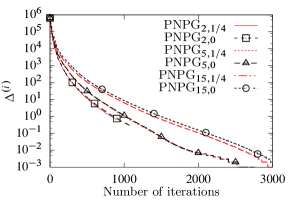
(a) $\ell_{1}$, $\boldsymbol{1}^{T}\Phi{\boldsymbol{x}}=10^{8}$, $a=0.5$

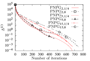
(b) TV, $\boldsymbol{1}^{T}\Phi{\boldsymbol{x}}=10^{7}$, $a=0$

Figure 4: Centered objectives of PNPG as functions of the CPU time for (a) $\ell_{1}$-norm and (b) TV regularizations.

In this example, we adopt the Poisson GLM (11a) with identity link in (12). Consider PET reconstruction of the $128\times 128$ concentration map ${\boldsymbol{x}}$ in Fig. 3(a), which represents simulated radiotracer activity in the human chest. Assume that the corresponding $128\times 128$ attenuation map $\boldsymbol{\kappa}$ is known, which is needed to model the attenuation of the gamma rays [43] and compute the sensing matrix $\Phi$ in this application. We collect the photons from $90$ equally spaced directions over $180\text{\,}\mathrm{\SIUnitSymbolDegree}$, with $128$ radial samples in each direction. Here, we adopt the parallel strip-integral matrix $\Gamma$ [44, Ch. 25.2] and use its implementation in the Image Reconstruction Toolbox (IRT) [45] with sensing matrix

$$\Phi=w\operatorname{diag}\bigl{(}\exp_{\circ}(-\Gamma\boldsymbol{\kappa}+{\boldsymbol{c}})\bigr{)}\Gamma$$ (45)

where ${\boldsymbol{c}}$ is a known vector generated using a zero-mean independent, identically distributed (i.i.d.) Gaussian sequence with variance $0.3$ to model the detector efficiency variation, and $w$ is a known scaling constant controlling the expected total number of detected photons due to true coincidence, $\boldsymbol{1}^{T}\operatorname{E}(\boldsymbol{y}-{\boldsymbol{b}})=\boldsymbol{1}^{T}\Phi{\boldsymbol{x}}$, which is a signal-to-noise ratio (SNR) measure. Here, we assume that the intercept term ${\boldsymbol{b}}$ (generally nonzero) is due to the background radiation, scattering effect, and accidental coincidence combined together; see also (12) the Poisson GLM. The elements of the intercept term have been set to a constant equal to $10\text{\,}\mathrm{\char 37\relax}$ of the sample mean of $\Phi{\boldsymbol{x}}$: ${\boldsymbol{b}}=\frac{\boldsymbol{1}^{T}\Phi{\boldsymbol{x}}}{10N}\boldsymbol{1}$.

The above model, choices of parameters in the PET system setup, and concentration map have been adopted from IRT [45, emission/em_test_setup.m].

Here, we consider both the $\ell_{1}$-norm with linear sparsifying transform [see (1a)] and isotropic TV penalties. For (1a), we construct a $p\times p^{\prime}=$12\,449\text{\times}14\,056$$ sparsifying dictionary matrix $\Psi$ with orthonormal rows [which satisfies (28)] using the 2-D Haar discrete wavelet transform (DWT) with $6$ decomposition levels and a full circular mask [46].

We compare the filtered backprojection (FBP) [43] and PG methods that aim at minimizing (3) with nonnegative $C$ in (2) and $\boldsymbol{\psi}({\boldsymbol{x}})$ in (1a) and (4): PNPG-$\ell_{1}$, PNPG-TV, AT-$\ell_{1}$, AT-TV, and SPIRAL-TV, where the suffixes “-$\ell_{1}$” and “-TV” denote the $\ell_{1}$-norm with linear sparsifying transform and TV penalties. We implemented SPIRAL-TV using the centered NLL term (11a), which improves the numerical stability compared with the original code in [41]. We do not compare with SPIRAL-$\ell_{1}$ because its inner iteration for the proximal step requires orthogonal (and hence square) $\Psi$, which is not the case here.

In this example, we adopt the following form of the regularization constant $u$:

$$u=10^{a}.$$ (46)

We vary $a$ in (46) in the range $[-6,3]$ with a grid size of $0.5$ and search for the reconstructions with the best average RSE performance. When possible, upper-bounding $u$ helps determine an appropriate search range for $u$; see [16] and [7, Th. LABEL:asil-thm:uMAX] for such upper bounds for $\ell_{1}$-norm and TV penalties, respectively.

All iterative methods were initialized by FBP reconstructions implemented by IRT [45]; see also [43].

Figs. 3(b)-3(d) show reconstructions for one random realization of the noise and detector variation ${\boldsymbol{c}}$, with the expected total annihilation photon count (SNR) equal to ${10}^{8}$; the optimal $a$ is 0.5. At this SNR, all sparse reconstruction methods compared (PNPG, AT, and SPIRAL) perform similarly as long as they employ the same penalty: the TV sparsity penalty is superior to the $\ell_{1}$-norm counterpart; see also Fig 6.

Figs. 4 and 5 show the centered objectives $\Delta^{(i)}$ as functions of CPU time for the $\ell_{1}$- and TV-norm signal sparsity regularizations and two random realizations of the noise and detector variation with different total expected photon counts. Fig. 4 examines the convergence of PNPG as a function of the momentum tuning constants $(\gamma,b)$ in (19), using $\gamma\in\{2,5,15\}$ and $b\in\{0,1/4\}$. For small $\gamma\leq 5$, there is no significant difference between different selections and no choice is uniformly the best, consistent with [40] which considers only $b=0$ and non-adaptive step size. As we increase $\gamma$ further ($\gamma=15$), we observe slower convergence. In the remainder of this section, we use $(\gamma,b)$ in (43).

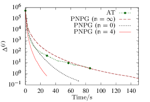
(a) $\ell_{1}$, $\boldsymbol{1}^{T}\Phi{\boldsymbol{x}}=10^{8}$, $a=0.5$

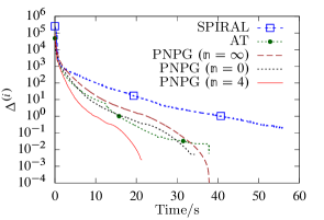
(b) TV, $\boldsymbol{1}^{T}\Phi{\boldsymbol{x}}=10^{7}$, $a=0$

Figure 5: Centered objectives as functions of the CPU time for (a) $\ell_{1}$-norm and (b) TV regularizations.

To illustrate the benefits of step-size adaptation, we present in Fig. 5 the performance of PNPG ($\mathbb{n}=\infty$), which does not adapt to the local curvature of the NLL, employs backtracking only, and has monotonically non-increasing step size, similar to FISTA. PNPG ($\mathbb{n}=\mathbb{m}=4$) outperforms PNPG ($\mathbb{n}=\infty$) because it uses step-size adaptation; see also Fig. 2(a) which corresponds to Fig. 5(a) and shows that the step size of PNPG ($\mathbb{n}=\mathbb{m}=4$) for the $\ell_{1}$-norm signal sparsity penalty is consistently larger than that of PNPG ($\mathbb{n}=\infty$). The advantage of PNPG ($\mathbb{n}=\mathbb{m}=4$) over the aggressive PNPG ($\mathbb{n}=\mathbb{m}=0$) scheme is due to the patient nature of its step-size adaptation, which leads to a better local majorization function of the NLL and reduces time spent backtracking. Indeed, if we do not account for the time spent on each iteration and only compare the objectives as functions of the iteration index, then PNPG ($\mathbb{n}=\mathbb{m}=4$) and PNPG ($\mathbb{n}=\mathbb{m}=0$) perform similarly; see [7, Fig. LABEL:asil-fig:tracePET]. Although PNPG ($\mathbb{n}=\mathbb{m}=0$) and AT have the same step-size selection strategy and $\mathcal{O}(k^{-2})$ convergence-rate guarantees, PNPG ($\mathbb{n}=\mathbb{m}=0$) converges faster; both schemes are further outperformed by PNPG ($\mathbb{n}=\mathbb{m}=4$). Fig. 5(b) shows that SPIRAL, which does not employ PG step acceleration, is at least 3 times slower than PNPG $({\mathbb{n}=\mathbb{m}=4})$ for the same convergence threshold in (42).

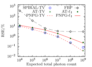
Figure 6: Minimum average RSEs as functions of $\boldsymbol{1}^{T}\Phi{\boldsymbol{x}}$.

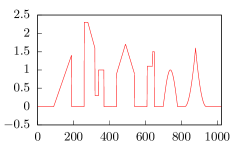
(a) true signal

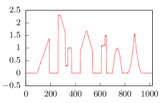
(b) PNPG

(c) NPG${}_{\text{S}}$

Figure 7: The true nonnegative skyline signal and its PNPG and NPG${}_{\text{S}}$ reconstructions for $N/p=0.34$.

Fig. 6 shows the minimum average (over 15 random realizations of the noise and detector variation ${\boldsymbol{c}}$) RSEs as functions of the expected total photon counts $\boldsymbol{1}^{T}\Phi{\boldsymbol{x}}\in\{10^{4},10^{5},\ldots,10^{9}\}$, where $a$ has been selected to minimize the average RSE for each method at each expected total photon count. For $\ell_{1}$-norm and TV regularizations, the optimal $a$ increases from $-0.5$ to $0.5$ and $-0.5$ to $1$, respectively, as we increase $\boldsymbol{1}^{T}\Phi{\boldsymbol{x}}$ from $10^{4}$ to $10^{9}$. As the SNR increases, FBP reaches a performance floor whereas PNPG, AT, and SPIRAL continue to improve thanks to the signal sparsity and nonnegativity constraints that they employ. The RSEs achieved by the methods that employ TV regularization are 1.2 to 6.3 times smaller than those achieved by $\ell_{1}$-norm regularization. As the SNR increases, the convergence points of SPIRAL-TV and PNPG-TV diverge, which explains the difference between the RSEs of the two methods at large SNRs in Fig. 6. This trend is already observed when $\boldsymbol{1}^{T}\operatorname{E}(\boldsymbol{y})=10^{7}$ in Fig. 5(b).

V-B Skyline Signal Reconstruction from Linear Measurements

We adopt the $\ell_{1}$-norm penalty with $\boldsymbol{\psi}(\cdot)$ in (1a) and linear measurement model with Gaussian noise in Section II-B where the elements of the sensing matrix $\Phi$ are i.i.d., drawn from the standard normal distribution. Due to the widespread use of this measurement model, we can compare wider range of methods than in the Poisson PET example in Section V-A.

We have designed a “skyline” signal of length $p=1024$ by overlapping magnified and shifted triangle, rectangle, sinusoid, and parabola functions; see Fig. 7(a). We generate the noiseless measurements using $\boldsymbol{y}=\Phi{\boldsymbol{x}}_{\text{true}}$. The DWT matrix $\Psi$ is constructed using the Daubechies-4 wavelet with 3 decomposition levels, whose approximation by the $5\text{\,}\mathrm{\char 37\relax}$ largest-magnitude wavelet coefficients achieves $\operatorname{RSE}=$98\text{\,}\mathrm{\char 37\relax}$$. We compare:

• AT, PNPG, and PNPG with continuation [47] (labeled PNPG (cont.));

• linearly constrained gradient projection method [4], part of the SPIRAL toolbox [41] and labeled SPIRAL herein;

• sparse reconstruction by separable approximation (SpaRSA) [48] with our implementation of the proximal mapping in Section III-C, inner convergence criterion with relative-error inner convergence criterion and convergence threshold in (44) (easy to incorporate into the SpaRSA software package [48] provided by the authors), and continuation (labeled SpaRSA (cont.));

• the GFB method [10]:

  $$\boldsymbol{z}_{1} \leftarrow \boldsymbol{z}_{1}+\lambda\bigl{[}\operatorname{prox}_{\frac{r}{w}u\lVert\Psi^{T}\cdot\rVert_{1}}\!\bigl{(}2{\boldsymbol{x}}-\boldsymbol{z}_{1}-r\nabla\mathcal{L}({\boldsymbol{x}})\bigr{)}-{\boldsymbol{x}}\bigr{]}$$

  $$\boldsymbol{z}_{2} \leftarrow \boldsymbol{z}_{2}+\lambda\bigl{[}P_{C}\bigl{(}2{\boldsymbol{x}}-\boldsymbol{z}_{2}-r\nabla\mathcal{L}({\boldsymbol{x}})\bigr{)}-{\boldsymbol{x}}\bigr{]}$$ (47b)

  $${\boldsymbol{x}} \leftarrow w\boldsymbol{z}_{1}+(1-w)\boldsymbol{z}_{2}$$ (47c)

  with $r=1.8/\lVert\Phi\rVert_{2}^{2}$, $\lambda=1$, and $w=0.5$ tuned for best performance, and

• the PDS method [11]:

  $$\bar{\boldsymbol{z}} \leftarrow P_{[-u,u]^{p}}\bigl{(}\boldsymbol{z}+\sigma\Psi^{T}{\boldsymbol{x}}\bigr{)}$$ (48a)

  $$\bar{{\boldsymbol{x}}} \leftarrow P_{C}\left({{\boldsymbol{x}}-\tau\nabla\mathcal{L}({\boldsymbol{x}})-\tau\Psi(2\bar{\boldsymbol{z}}-\boldsymbol{z})}\right)$$ (48b)

  $$\boldsymbol{z} \leftarrow \boldsymbol{z}+\rho(\bar{\boldsymbol{z}}-\boldsymbol{z})$$ (48c)

  $${\boldsymbol{x}} \leftarrow {\boldsymbol{x}}+\rho(\bar{{\boldsymbol{x}}}-{\boldsymbol{x}})$$ (48d)

  where $\tau$ and $\sigma$ are related as follows: $\tau(\sigma+\lVert\Phi\rVert_{2}^{2}/2)=1$, with $\sigma=\tau$ and $\rho=2-0.5\lVert\Phi\rVert_{2}^{2}\bigl{(}{1}/{\tau}-\sigma\bigr{)}^{-1}$ tuned for best performance,

all of which aim to solve the generalized analysis BPDN problem with a convex signal constraint; the implementations of the GFB and PDS methods in (47) and (48) correspond to this scenario. Here, $p^{\prime}=p$, $\Psi$ is an orthogonal matrix ($\Psi\Psi^{T}=\Psi^{T}\Psi=I$), and $\operatorname{prox}_{\lambda\lVert\Psi^{T}\cdot\rVert_{1}}{\boldsymbol{a}}=\Psi\operatorname{\mathcal{T}}_{\lambda}\bigl{(}\Psi^{T}{\boldsymbol{a}}\bigr{)}$ has a closed-form solution (see (7c)), which simplifies the implementation of the GFB method ((47), in particular); see the discussion in Section I. The other tuning options for SPIRAL, SpaRSA (cont.), and AT are kept to their default values, unless specified otherwise.

We initialize the iterative methods by the approximate minimum-norm estimate: ${\boldsymbol{x}}^{(0)}=\Phi^{T}[\operatorname{E}(\Phi\Phi^{T})]^{-1}\boldsymbol{y}=\Phi^{T}\boldsymbol{y}/p$. and select the regularization parameter $u$ as

$$u=10^{a}U, U\triangleq\lVert\Psi^{T}\nabla\mathcal{L}(\boldsymbol{0})\rVert_{\infty}$$ (49)

where $a$ is an integer selected from the interval $[-9,-1]$ and $U$ is an upper bound on $u$ of interest. Indeed, the minimum point ${\boldsymbol{x}}^{\star}$ in (33a) reduces to $\boldsymbol{0}$ if $u\geq U$ [16, Sec. LABEL:report-sec:adaptivecontinuation].

As before, PNPG ($\mathbb{n}=\mathbb{m}=4$) and PNPG ($\mathbb{n}=\mathbb{m}=0$) converge at similar rates as functions of the number of iterations. However, due to the excessive attempts to increase the step size at every iteration, PNPG ($\mathbb{n}=\mathbb{m}=0$) spends more time backtracking and converges at a slower rate as a function of CPU time compared with PNPG ($\mathbb{n}=\mathbb{m}=4$); see also Fig. 2(b) which corresponds to Fig. 8(b) and shows the step sizes as functions of the number of iterations for $a=-4$ and $N/p=0.34$. Hence, we present only the performances of PNPG with $\mathbb{n}=\mathbb{m}=4$ in this section.

Fig. 7 shows the advantage brought by the convex-set nonnegativity signal constraints (2). Figs. 7(b) and 7(c) present the PNPG $(a=-5)$ and NPG${}_{\text{S}}$ $(a=-4)$ reconstructions from one realization of the linear measurements with $N/p=0.34$ and $a$ tuned for the best RSE performance. Recall that NPG${}_{\text{S}}$ imposes signal sparsity only. Here, imposing signal nonnegativity improves greatly the overall reconstruction and does not simply rectify the signal values close to zero.

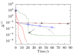
(a) $a=-5,N/p=0.34$

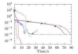
(b) $a=-4,N/p=0.34$

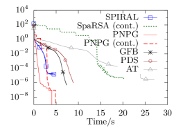
(c) $a=-3,N/p=0.34$

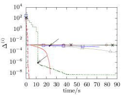
(d) $a=-6,N/p=0.49$

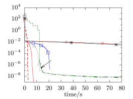
(e) $a=-5,N/p=0.49$

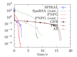
(f) $a=-4,N/p=0.49$

Figure 8: Centered objectives as functions of CPU time for normalized numbers of measurements $N/p\in\{0.34,0.49\}$ and different regularization constants $a$.

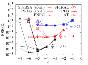
Figure 9: Average RSEs as functions of the regularization constant $a$.

Fig. 8 presents the centered objectives $\Delta^{(i)}$ as functions of CPU time for two random realizations of the sensing matrix $\Phi$ with different normalized numbers of measurements $N/p$ (in top and bottom rows, respectively) and several regularization constants $a$. The scenario with small $a$ is challenging for all optimization methods and the remedy is to use continuation. We present the performance of the PNPG method both with and without continuation, labeled PNPG and PNPG (cont.), respectively. SpaRSA without continuation performs poorly and hence we apply only its version with continuation throughout this section. We illustrate the benefits of continuation to the convergence of the PNPG scheme when $a$ is small. Note that the “knee” in the SpaRSA (cont.) performance curve occurs at the place where its continuation is completed, i.e., the regularization parameter for continuation descends to $u$. This phenomenon is observed in all 20 trials. Indeed, upon completion of continuation, SpaRSA (cont.) is simply a PG scheme without acceleration, which explains its low convergence rate following the “knee”; we run SpaRSA (cont.) beyond its point of convergence mandated by (42) and mark by arrows its convergence points for the convergence threshold in (42). Similarly, AT conveges prematurely in Fig. 8(d), where its convergence point is marked by an arrow.

All methods in Fig. 8 converge more slowly as $a$ decreases. GFB, PDS, and SPIRAL are especially vulnerable to small $a$; see Figs. 8(a) and 8(d). Thanks to continuation, SpaRSA (cont.) and PNPG (cont.) have more stable CPU times for different $a$s compared with the methods that do not employ continuation; PNPG (cont.) is slightly slower than PNPG when $a$ is large.

Among the methods that do not employ continuation, PNPG has the steepest descent rate, followed by SPIRAL and AT. AT uses 2 to 10 times more CPU time to reach the same objective than PNPG. This justifies our convex-set projection in (17d) for the Nesterov’s acceleration step [17, 18], shows superiority of (17d) over AT’s acceleration in (40a) and (40c), and is consistent with the results in the Poisson example in Section V-A.

In Fig. 9, we show the average RSEs (over 20 random realizations of the sensing matrix) as functions of the regularization parameter $a$ for normalized numbers of measurements $N/p\in\{0.24,0.34,0.49\}$, which are coded by blue, black, and red colors, respectively. PDS and GFB perform approximately the same, hence we show only the performance of PDS. PNPG (cont.) achieves the smallest RSEs for all $a$, followed by SpaRSA (cont.), where the gap between the two methods is due to the fact that SpaRSA (cont.) converges prematurely.

PNPG (cont.) achieves the smallest RSEs and is particularly effective for small $a$. PNPG struggles when $a$ is small, thus emphasizing the importance of continuation in this scenario. SPIRAL and PDS have similar performance and start to fail earlier than PNPG as $a$ decreases and, for small $a$, yields reconstructions with much larger RSEs than PNPG. AT fails when $a<-5$ because it converges prematurely; see also Fig. 8(d).

The methods that have large RSE (around $10\text{\,}\mathrm{\char 37\relax}$) and effectively fail would not achieve better RSE even if they use more stringent convergence criteria than (42).

VI Conclusion

We developed a fast algorithm for reconstructing signals that are sparse in a transform domain and belong to a closed convex set by employing a projected proximal-gradient scheme with Nesterov’s acceleration, restart and adaptive step size. We applied the proposed framework to construct the first Nesterov-accelerated Poisson compressed-sensing reconstruction algorithm. We presented integrated derivation of the proposed algorithm and convergence-rate upper-bound that accounts for inexactness of the proximal operator and also proved convergence of iterates. Our PNPG approach is computationally efficient compared with the state-of-the-art.

Appendix A Derivation of Acceleration (17a)–(17d) and
Proofs of Lemma 1 and Theorem 1

We first prove Lemma 1 and then derive the acceleration (17a)–(17d) and prove Theorem 1.

Proof:

According to Definition 1 and (20),

$$ur({\boldsymbol{x}}) \geq ur({\boldsymbol{x}}^{(i)})+({\boldsymbol{x}}-{\boldsymbol{x}}^{(i)})^{T}\biggl{[}\frac{{\overline{{\boldsymbol{x}}}}^{(i)}-{\boldsymbol{x}}^{(i)}}{\beta^{(i)}}-\nabla\mathcal{L}({\overline{{\boldsymbol{x}}}}^{(i)})\biggr{]}$$ (A1a)

$$\qquad-\>\frac{(\varepsilon^{(i)})^{2}}{2\beta^{(i)}}$$

for any $${\boldsymbol{x}}\in\mathamsbb{R}^{p} \mathcal{L}({\boldsymbol{x}})$$. Moreover, due to the convexity of , we have

$$\mathcal{L}({\boldsymbol{x}}) \geq \mathcal{L}({\overline{{\boldsymbol{x}}}}^{(i)})+({\boldsymbol{x}}-{\overline{{\boldsymbol{x}}}}^{(i)})^{T}\nabla\mathcal{L}({\overline{{\boldsymbol{x}}}}^{(i)}).$$ (A1b)

Summing (A1a), (A1b), and (18) completes the proof. ∎

The following result from [49, Proposition 2.2.1] states that the distance between ${\boldsymbol{x}}$ and $\boldsymbol{y}$ can be reduced by projecting them onto a closed convex set $C$.

Lemma 2 (Projection theorem)

The projection mapping onto a nonempty closed convex set $C\subseteq\mathamsbb{R}^{p}$ is nonexpansive

$$\lVert P_{C}({\boldsymbol{x}})-P_{C}(\boldsymbol{y})\rVert^{2}_{2}\leq\lVert{\boldsymbol{x}}-\boldsymbol{y}\rVert^{2}_{2}$$ (A2)

for all ${\boldsymbol{x}},\boldsymbol{y}\in\mathamsbb{R}^{p}$.

We now derive the Nesterov’s acceleration step (17b)–(17d) with goal to select ${\overline{{\boldsymbol{x}}}}^{(i)}$ in (17e) that achieves the convergence rate of $\mathcal{O}(k^{-2})$.

Define sequences $a^{(i)}>0$ and $b^{(i)}>0$, multiply them with (34a) and (34b), respectively, add the resulting expressions, and multiply by $\beta^{(i)}$ to obtain

$$\IEEEeqnarraymulticol{3}{l}{-2\beta^{(i)}c^{(i)}\Delta^{(i)}+2\beta^{(i)}b^{(i)}\Delta^{(i-1)}}$$ (A3)

$$\geq \frac{1}{c^{(i)}}\bigl{\|}c^{(i)}{\boldsymbol{x}}^{(i)}-b^{(i)}{\boldsymbol{x}}^{(i-1)}-a^{(i)}{\boldsymbol{x}}^{\star}\bigr{\|}_{2}^{2}$$

$$\qquad-\>\frac{1}{c^{(i)}}\bigl{\|}c^{(i)}{\overline{{\boldsymbol{x}}}}^{(i)}-b^{(i)}{\boldsymbol{x}}^{(i-1)}-a^{(i)}{\boldsymbol{x}}^{\star}\bigr{\|}_{2}^{2}-c^{(i)}(\varepsilon^{(i)})^{2}$$

$$= c^{(i)}\bigl{[}t^{(i)}-\bar{t}^{(i)}-(\varepsilon^{(i)})^{2}\bigr{]}$$

where

$$c^{(i)} \triangleq a^{(i)}+b^{(i)}$$ (A4a)

$$t^{(i)} \triangleq \lVert{\boldsymbol{x}}^{(i)}-\boldsymbol{z}^{(i)}\rVert_{2}^{2},\qquad\bar{t}^{(i)}\triangleq\lVert{\overline{{\boldsymbol{x}}}}^{(i)}-\boldsymbol{z}^{(i)}\rVert_{2}^{2}$$ (A4b)

$$\boldsymbol{z}^{(i)} \triangleq \frac{b^{(i)}}{c^{(i)}}{\boldsymbol{x}}^{(i-1)}+\frac{a^{(i)}}{c^{(i)}}{\boldsymbol{x}}^{\star}.$$ (A4c)

We arranged (A3) using completion of squares so that the first two summands are similar (but with opposite signs), with goal to facilitate cancellations as we sum over $i$. Since we have control over the sequences $a^{(i)}$ and $b^{(i)}$, we impose the following conditions for $i\geq 1$:

$${c^{(i-1)}}t^{(i-1)} \geq {c^{(i)}}\bar{t}^{(i)}$$ (A5a)

$$\pi^{(i)} \geq 0$$ (A5b)

where

$$\pi^{(i)} \triangleq \beta^{(i)}c^{(i)}-\beta^{(i+1)}b^{(i+1)}.$$ (A6)

Now, apply the inequality (A5a) to the right-hand sides of (A3):

$$-{2\beta^{(i)}}c^{(i)}\Delta^{(i)}+{2\beta^{(i)}}b^{(i)}\Delta^{(i-1)} \geq {c^{(i)}}t^{(i)}-{c^{(i-1)}}t^{(i-1)}$$ (A7a)

$$\kern 5.0pt-\>c^{(i)}(\varepsilon^{(i)})^{2}$$

and sum (A7a) over $$i=1,2,\ldots,k$$, which leads to summand cancellations and

$$\IEEEeqnarraymulticol{3}{l}{-{2\beta^{(k)}}c^{(k)}\Delta^{(k)}+2\beta^{(1)}b^{(1)}\Delta^{(0)}-2\sum_{i=1}^{k-1}\pi^{(i)}\Delta^{(i)}}$$ (A7c)

$$\kern 30.0pt\geq{c^{(k)}}t^{(k)}-{c^{(0)}}t^{(0)}-\sum_{i=1}^{k}c^{(i)}(\varepsilon^{(i)})^{2}$$

$$\kern 30.0pt\geq-{c^{(0)}}t^{(0)}-\sum_{i=1}^{k}c^{(i)}(\varepsilon^{(i)})^{2}$$

and (A7c) follows from (A7c) by discarding the nonnegative term $$c^{(k)}t^{(k)}$$.

Now, due to $\pi^{(i)}\Delta^{(i)}\geq 0$, the inequality (A7c) leads to

$$\Delta^{(k)}\leq\frac{2\beta^{(1)}b^{(1)}\Delta^{(0)}+{c^{(0)}}t^{(0)}+\sum_{i=1}^{k}c^{(i)}(\varepsilon^{(i)})^{2}}{2\beta^{(k)}c^{(k)}}$$ (A8)

with simple upper bound on the right-hand side, thanks to summand cancellations facilitated by the assumptions (A5).

As long as $\beta^{(k)}c^{(k)}$ grows at a rate of $k^{2}$ and the inaccuracy of the proximal mappings leads to bounded $\sum_{i=1}^{k}c^{(i)}(\varepsilon^{(i)})^{2}$, the centered objective function $\Delta^{(k)}$ can achieve the desired bound decrease rate of $1/k^{2}$. Now, we discuss how to satisfy (A5) and the growth rate of $\beta^{(k)}c^{(k)}$ by an appropriate selection of ${\overline{{\boldsymbol{x}}}}^{(i)}$.

A-I Satisfying Conditions (A5)

A-Ia Imposing equality in (A5a)

(A5a) holds with equality for all $i$ and any ${\boldsymbol{x}}^{\star}$ when we choose ${\overline{{\boldsymbol{x}}}}^{(i)}=\widehat{{\boldsymbol{x}}}^{(i)}$ that satisfy

$$\sqrt{c^{(i-1)}}({\boldsymbol{x}}^{(i-1)}-\boldsymbol{z}^{(i-1)})={\sqrt{c^{(i)}}}(\widehat{{\boldsymbol{x}}}^{(i)}-\boldsymbol{z}^{(i)}).$$ (A9)

Now, (A9) requires equal coefficients multiplying ${\boldsymbol{x}}^{\star}$ on both sides, thus ${a^{(i)}}/{\sqrt{c^{(i)}}}=1/\mathrm{w}$ for all $i$, where $\mathrm{w}>0$ is a constant (not a function of $i$), which implies $c^{(i)}=\mathrm{w}^{2}(a^{(i)})^{2}$ and $b^{(i)}=\mathrm{w}^{2}(a^{(i)})^{2}-a^{(i)}$, see also (A4a). Upon defining

$$\theta^{(i)}\triangleq\mathrm{w}^{2}a^{(i)}$$ (A10a)

we have

$$\mathrm{w}^{2}c^{(i)}=(\theta^{(i)})^{2}, \mathrm{w}^{2}b^{(i)}=(\theta^{(i)})^{2}-\theta^{(i)}.$$ (A10b)

Plug (A10) into (A9) and reorganize to obtain the following form of momentum acceleration:

$$\widehat{{\boldsymbol{x}}}^{(i)}={\boldsymbol{x}}^{(i-1)}+\Theta^{(i)}({\boldsymbol{x}}^{(i-1)}-{\boldsymbol{x}}^{(i-2)}).$$ (A11)

Although ${\overline{{\boldsymbol{x}}}}^{(i)}=\widehat{{\boldsymbol{x}}}^{(i)}$ satisfies (A5a), it is not guaranteed to be within $\operatorname{dom}\mathcal{L}$; consequently, the proximal-mapping step for this selection may not be computable.

A-Ib Selecting ${\overline{{\boldsymbol{x}}}}^{(i)}\in C$ that satisfies (A5a)

We now seek ${\overline{{\boldsymbol{x}}}}^{(i)}$ within $C$ that satisfies the inequality (A5a). Since ${\boldsymbol{x}}^{(i-1)}$ and ${\boldsymbol{x}}^{\star}$ are in $C$, $\boldsymbol{z}^{(i)}\in C$ by the convexity of $C$; see (A4c). According to Lemma 2, projecting (A11) onto $C$ preserves or reduces the distance between points. Therefore,

$${\overline{{\boldsymbol{x}}}}^{(i)}=P_{C}(\widehat{{\boldsymbol{x}}}^{(i)})$$ (A12)

belongs to $C$ and satisfies the condition (A5a):

$${c^{(i-1)}}t^{(i-1)} = {c^{(i)}}\lVert\widehat{{\boldsymbol{x}}}^{(i)}-\boldsymbol{z}^{(i)}\rVert_{2}^{2}$$ (A13a)

$$\geq {c^{(i)}}\lVert{\overline{{\boldsymbol{x}}}}^{(i)}-\boldsymbol{z}^{(i)}\rVert_{2}^{2}={c^{(i)}}\bar{t}^{(i)}$$ (A13b)

where (A13a) and (A13b) follow from (A9) and by using Lemma 2, respectively; see also (A4b).

Without loss of generality, set $\mathrm{w}=1$ and rewrite and modify (A6), (A4b), and (A7c) using (A10) to obtain

$$\pi^{(i)} = \beta^{(i)}(\theta^{(i)})^{2}$$ (A14a)

$$-\>\beta^{(i+1)}\theta^{(i+1)}\bigl{(}\theta^{(i+1)}-1\bigr{)},\;\;i\geq 1$$

$$(\theta^{(i)})^{2}{t}^{(i)} = \bigl{\|}\theta^{(i)}{\boldsymbol{x}}^{(i)}-\bigl{(}\theta^{(i)}-1\bigr{)}{\boldsymbol{x}}^{(i-1)}-{\boldsymbol{x}}^{\star}\bigr{\|}_{2}^{2}$$ (A14b)

$$\sum_{i=1}^{k-1}\pi^{(i)}\Delta^{(i)} \leq \frac{1}{2}\Bigl{[}(\theta^{(0)})^{2}t^{(0)}+\sum_{i=1}^{k}(\theta^{(i)}\varepsilon^{(i)})^{2}\Bigr{]}$$ (A14c)

where (A14c) is obtained by discarding the negative term $-2\beta^{(k)}(\theta^{(k)})^{2}\Delta^{(k)}$ and the zero term $\beta^{(1)}\theta^{(1)}(\theta^{(1)}-1)\Delta^{(0)}$ (because $\theta^{(1)}=1$) on the left-hand side of (A7c). Now, (32a) follows from (A8) by using $\theta^{(0)}=\theta^{(1)}=1$ (see (17b)), (A10), and (A14b) with $i=0$.

A-Ic Satisfying (A5b)

By substituting (A14a) into (A5b), we obtain the conditions (35a) and interpret $\bigl{(}\pi^{(i)}\bigr{)}_{i=1}^{+\infty}$ as the sequence of gaps between the two sides of (35a).

A-II Connection to Convergence-Rate Analysis of FISTA

If the step-size sequence $(\beta^{(i)})$ is non-increasing (e.g., in the backtracking-only scenario with $\mathbb{n}=+\infty$), (17b) with $B^{(i)}=1$ also satisfies the inequality (35b). In this case, (32a) still holds but (32b) does not because (36b) no longer holds. However, because $B^{(i)}=1$, we have $\theta^{(k)}\geq\frac{k+1}{2}$ and

$$\Delta^{(k)} \leq \gamma^{2}\frac{\bigl{\|}{\boldsymbol{x}}^{(0)}-{\boldsymbol{x}}^{\star}\bigr{\|}^{2}_{2}+\mathcal{E}^{(k)}}{2\beta^{(k)}(k+1)^{2}}$$ (A15)

which generalizes [18, Th. 4.4] to include the inexactness of the proximal operator and the convex-set projection.

Appendix B Convergence of Iterates

To prove convergence of iterates, we need to show that the centered objective function $\Delta^{(k)}$ decreases faster than the right-hand side of (32b). We introduce Lemmas 3 and 4 and then use them to prove Theorem 2. Throughout this Appendix, we assume that Assumption 1) of Theorem 2 holds, which justifies (34) and (35) as well as results from Appendix A that we use in the proofs.

Lemma 3

Under Assumptions 1)–3) of Theorem 2,

$$\sum_{i=1}^{+\infty}\bigl{(}2\theta^{(i)}-1\bigr{)}\delta^{(i)}<+\infty.$$ (B1)

Proof:

By letting $k\rightarrow+\infty$ in (A14c) and using (38), we obtain

$$\sum_{i=1}^{+\infty}\pi^{(i)}\Delta^{(i)}<+\infty.$$ (B2)

For $i\geq 1$, rewrite (A14a) using $\theta^{(i)}$ expressed in terms of $\theta^{(i+1)}$ (based on (17b)):

$${\pi^{(i)}} = \frac{\beta^{(i+1)}}{\gamma}\Bigl{[}(\gamma-2)\theta^{(i+1)}+\frac{1-b\gamma^{2}}{\gamma}\Bigr{]}$$ (B3)

$$\geq \frac{\gamma-2}{\gamma}\beta^{(i+1)}\theta^{(i+1)}$$

where the inequality in (B3) is due to $b\gamma^{2}-1<0$; see Assumption 3). Apply nonexpansiveness of the projection operator to (34b) and use (A11) to obtain

$${2\beta^{(i)}}(\Delta^{(i-1)}-\Delta^{(i)}) \geq \delta^{(i)}-(\Theta^{(i)})^{2}\delta^{(i-1)}-(\varepsilon^{(i)})^{2}$$ (B4)

then multiply both sides of (B4) by $(\theta^{(i)})^{2}$, sum over $i=1,2,\ldots,k$ and reorganize:

$$\IEEEeqnarraymulticol{3}{l}{\sum_{i=1}^{k-1}(2\theta^{(i)}-1)\delta^{(i)}\leq(\theta^{(0)}-1)^{2}\delta^{(0)}-(\theta^{(k)})^{2}\delta^{(k)}+2\beta^{(1)}\Delta^{(0)}}$$ (B5a)

$$+\>\mathcal{E}^{(k)}+2\sum_{i=1}^{k-1}\rho^{(i)}\Delta^{(i)}$$

$$\leq 2\beta^{(1)}\Delta^{(0)}+\mathcal{E}^{(k)}+\frac{4}{\gamma-2}\sum_{i=1}^{k-1}\pi^{(i)}\Delta^{(i)}$$ (B5b)

where (see (A14a))

$$\rho^{(i)} = \beta^{(i+1)}(\theta^{(i+1)})^{2}-\beta^{(i)}(\theta^{(i)})^{2}$$ (B5c)

$$= \beta^{(i+1)}\theta^{(i+1)}-\pi^{(i)},$$ (B5d)

and we drop the zero term $\bigl{(}\theta^{(0)}-1\bigr{)}^{2}\delta^{(0)}$ and the negative term $-\bigl{(}\theta^{(k)}\bigr{)}^{2}\delta^{(k)}$ from (B5a) and use the fact that $\rho^{(i)}\leq\tfrac{2}{\gamma-2}\pi^{(i)}$ implied by (B3) to get (B5b). Finally, let $k\rightarrow+\infty$ and use (38) and (B2) to conclude (B1). ∎

Lemma 4

For $j\geq 3$,

$$\Pi_{j}\triangleq\sum_{k=j}^{+\infty}\prod_{\ell=j}^{k}\Theta^{(\ell)} \leq \gamma\theta^{(j-1)}-1.$$ (B6)

Proof:

For $j\geq 3$,

$$\frac{1}{\sqrt{\beta^{(k-1)}}\theta^{(k-1)}\theta^{(k)}} \leq \frac{\gamma}{\sqrt{\beta^{(k-1)}}\theta^{(k-1)}}-\frac{\gamma}{\sqrt{\beta^{(k)}}\theta^{(k)}}\qquad$$ (B7a)

$$\leq \frac{\gamma}{\sqrt{\beta^{(k-2)}}\theta^{(k-2)}}-\frac{\gamma}{\sqrt{\beta^{(k)}}\theta^{(k)}}$$ (B7b)

where we obtain the inequality (B7a) by combining the terms on the right-hand size and using (36a) and (B7b) holds because $\sqrt{\beta^{(k)}}\theta^{(k)}$ is an increasing sequence (see Section IV). Now,

$$\Pi_{j} \leq \sum_{k=j}^{+\infty}\prod_{\ell=j}^{k}\frac{\beta^{(\ell-2)}\bigl{(}\theta^{(\ell-2)}\bigr{)}^{2}}{\beta^{(\ell-1)}\theta^{(\ell-1)}\theta^{(\ell)}}=\sum_{k=j}^{+\infty}\frac{\beta^{(j-2)}\bigl{(}\theta^{(j-2)}\bigr{)}^{2}\theta^{(j-1)}}{\beta^{(k-1)}\bigl{(}\theta^{(k-1)}\bigr{)}^{2}\theta^{(k)}}$$

$$\IEEEeqnarraymulticol{3}{l}{\leq\frac{\gamma\beta^{(j-2)}\bigl{(}\theta^{(j-2)}\bigr{)}^{2}\theta^{(j-1)}}{\sqrt{\beta^{(j-2)}}\theta^{(j-2)}\sqrt{\beta^{(j-1)}}\theta^{(j-1)}}=\gamma\sqrt{B^{(j-1)}}\theta^{(j-2)}}$$ (B8b)

where (B8) follows by using (17c), (35a) with $i=\ell-1$, and fraction-term cancellation; (B8b) is obtained by substituting (B7b) into (B8) and canceling summation terms. (B8b) implies (B6) by using (36a) with $k=j-1$. ∎

Define

$$\lambda^{(i)}\triangleq\lVert{\boldsymbol{x}}^{(i)}-{\boldsymbol{x}}^{\star}\rVert_{2}^{2}, \Lambda^{(i)}\triangleq\lambda^{(i)}-\lambda^{(i-1)}.$$ (B9)

Since $f({\boldsymbol{x}}^{(i)})$ converges to $f({\boldsymbol{x}}^{\star})=\min_{\boldsymbol{x}}f({\boldsymbol{x}})$ as the iteration index $i$ grows and ${\boldsymbol{x}}^{\star}$ is a minimizer, it is sufficient to prove the convergence of $\lambda^{(i)}$, see [40, Th. 4.1].

Proof:

Use (34a) and the fact that $\Delta^{(i)}\geq 0$ to get

$$0 \geq \lambda^{(i)}-\lVert{\overline{{\boldsymbol{x}}}}^{(i)}-{\boldsymbol{x}}^{\star}\rVert_{2}^{2}-(\varepsilon^{(i)})^{2}.$$ (B10)

Now,

$$\IEEEeqnarraymulticol{3}{l}{\lVert{\overline{{\boldsymbol{x}}}}^{(i)}-{\boldsymbol{x}}^{\star}\rVert_{2}^{2}\leq\lVert\widehat{{\boldsymbol{x}}}^{(i)}-{\boldsymbol{x}}^{\star}\rVert_{2}^{2}=\lambda^{(i-1)}+(\Theta^{(i)})^{2}\delta^{(i-1)}}$$ (B11a)

$$\;+\>2\Theta^{(i)}({\boldsymbol{x}}^{(i-1)}-{\boldsymbol{x}}^{\star})^{T}({\boldsymbol{x}}^{(i-1)}-{\boldsymbol{x}}^{(i-2)})$$

$$\leq \lambda^{(i-1)}+(\Theta^{(i)})^{2}\delta^{(i-1)}+\Theta^{(i)}(\Lambda^{(i-1)}+\delta^{(i-1)})$$ (B11b)

where (B11a) and (B11b) follow by using the nonexpansiveness of the projection operator (see also (A11)) and the identity

$$2({\boldsymbol{a}}-{\boldsymbol{b}})^{T}({\boldsymbol{a}}-{\boldsymbol{c}})=\lVert{\boldsymbol{a}}-{\boldsymbol{b}}\rVert^{2}_{2}+\lVert{\boldsymbol{a}}-{\boldsymbol{c}}\rVert_{2}^{2}-\lVert{\boldsymbol{b}}-{\boldsymbol{c}}\rVert_{2}^{2}$$ (B12)

respectively. Combine the inequalities (B11b) and (B10) to get

$$\Lambda^{(i)} \leq \Theta^{(i)}\bigl{[}\Lambda^{(i-1)}+\bigl{(}\Theta^{(i)}+1\bigr{)}\delta^{(i-1)}\bigr{]}+(\varepsilon^{(i)})^{2}$$ (B13a)

$$\leq \Theta^{(i)}\bigl{(}\Lambda^{(i-1)}+{2\delta^{(i-1)}}/{\xi}\bigr{)}+(\varepsilon^{(i)})^{2}$$ (B13b)

where (B13b) is due to $1<\frac{1}{{\xi}}$ (see (26b)) and the following

$$\Theta^{(i)} < \frac{\theta^{(i-1)}}{\theta^{(i)}}=\frac{\sqrt{\beta^{(i-1)}}\theta^{(i-1)}\sqrt{\beta^{(i)}}}{\sqrt{\beta^{(i)}}\theta^{(i)}\sqrt{\beta^{(i-1)}}}$$ (B14a)

$$< \frac{\sqrt{\beta^{(i)}}}{\sqrt{\beta^{(i-1)}}}\leq\frac{1}{\sqrt{\xi}}<\frac{1}{{\xi}}$$ (B14b)

where we have used (17c) and that $\sqrt{\beta^{(i)}}\theta^{(i)}$ is an increasing sequence, $\beta^{(i)}/\beta^{(i-1)}\geq 1/\xi$ (see Section III-B), and (26b).

According to (36b) and Assumption 4) that the sequence $(\beta^{(i)})$ is bounded, there exists an integer $J$ such that

$$\theta^{(j-1)}\geq 2, \Theta^{(j)}\geq\frac{1}{\theta^{(j)}}>0$$ (B15)

for all $j\geq J$, where the second inequality follows from the first and the definition of $\Theta^{(j)}$, see (17c). Then

$$\Omega^{(i)} \triangleq \max(0,\Lambda^{(i)})\leq\Theta^{(i)}\biggl{[}\Omega^{(i-1)}+\frac{2\delta^{(i-1)}}{\xi}+\frac{(\varepsilon^{(i)})^{2}}{\Theta^{(i)}}\biggr{]}$$

$$\IEEEeqnarraymulticol{3}{l}{\leq\sum_{j=J}^{i}\biggl{[}\frac{2\delta^{(j-1)}}{\xi}+\frac{(\varepsilon^{(j)})^{2}}{\Theta^{(j)}}\biggr{]}\prod_{\ell=j}^{i}\Theta^{(\ell)}+\Omega^{(J-1)}\prod_{\ell=J}^{i}\Theta^{(\ell)}}$$ (B16b)

for $i\geq J$, where the inequality in (B16) follows by combining the inequalities (B13b) and $\Omega^{(i-1)}\geq\Lambda^{(i-1)}$ and (B16b) follows by recursively applying inequality (B16) with $i$ replace by $i-1,i-2,\ldots,J$. Now, sum the inequalities (B16b) over $i=J,J+1,\ldots,+\infty$ and exchange the order of summation over $i$ and $j$ on the right-hand side:

$$\sum_{i=J}^{+\infty}\Omega^{(i)} \leq \sum_{j=J}^{+\infty}\Pi_{j}\biggl{[}\frac{2\delta^{(j-1)}}{\xi}+\frac{(\varepsilon^{(j)})^{2}}{\Theta^{(j)}}\biggr{]}+\Pi_{J}\Omega^{(J-1)}$$ (B17)

where $\Pi_{j}$ is defined in Lemma 4.

For $j\geq J\geq 3$,

$$\gamma\,(2\theta^{(j-1)}-1)-\Pi_{j} \geq \gamma\,(\theta^{(j-1)}-1)+1>0$$ (B18a)

$$2\,\gamma\,(\theta^{(j-1)}-1)-\Pi_{j} \geq \gamma\,(\theta^{(j-1)}-2)+1>0$$ (B18b)

where the first and second inequalities in (B18) follow by applying Lemma 4 and (B15), respectively; consequently,

$$\sum_{j=J}^{+\infty}\Pi_{j}\delta^{(j-1)} \leq \gamma\sum_{j=J}^{+\infty}(2\theta^{(j)}-1)\delta^{(j)}<+\infty$$ (B19a)

$$\sum_{j=J}^{+\infty}\Pi_{j}\frac{(\varepsilon^{(j)})^{2}}{\Theta^{(j)}} \leq 2\gamma\sum_{j=J}^{+\infty}(\varepsilon^{(j)})^{2}\frac{\theta^{(j-1)}-1}{\Theta^{(j)}}$$ (B19b)

$$= 2\gamma\sum_{j=J}^{+\infty}(\varepsilon^{(j)})^{2}{\theta^{(j)}}$$ (B19c)

$$\leq 2\gamma\sum_{j=J}^{+\infty}(\theta^{(j)}\varepsilon^{(j)})^{2}$$ (B19d)

where (B19a) follows from (B18a) and Lemma 3 (for the second inequality) and (B19b) follows by using (B18b); (B19c) and (B19d) are due to (17c) and (B15), respectively. Combine (B19a) and (B19d) with (B17) to conclude that

$$\sum_{i=1}^{+\infty}\Omega^{(i)} < +\infty.$$ (B20)

The remainder of the proof uses the technique employed by [40] to conclude the proof of [40, Th. 4.1 at p. 978], which we repeat for completeness. Define $X^{(i)}\triangleq\lambda^{(i)}-\sum_{j=1}^{i}\Omega^{(j)}$, which is lower-bounded because $\lambda^{(i)}$ and $\sum_{j=1}^{i}\Omega^{(j)}$ are lower- and upper-bounded (by (B20)), respectively. Furthermore, $\bigl{(}X^{(i)}\bigr{)}$ is an non-increasing sequence:

$$X^{(i+1)} = \lambda^{(i+1)}-\Omega^{(i+1)}-\sum_{j=1}^{i}\Omega^{(j)}\leq X^{(i)},$$ (B21)

where we used the fact that $\Omega^{(i+1)}\geq\Lambda^{(i+1)}=\lambda^{(i+1)}-\lambda^{(i)}$. Hence, $\bigl{(}X^{(i)}\bigr{)}$ converges as $i\rightarrow+\infty$. Since $\sum_{j=1}^{i}\Omega^{(j)}$ converges, $(\lambda^{(i)})$ also converges. ∎

References

- [1] Emmanuel J Candes and Terence Tao “Near-optimal signal recovery from random projections: Universal encoding strategies?” In IEEE Trans. Inf. Theory 52.12, 2006, pp. 5406–5425
- [2] Jerry L Prince and Jonathan M Links “Medical Imaging Signals and Systems” Upper Saddle River, NJ: Pearson, 2015
- [3] Z T Harmany, R F Marcia and R M Willett “This is SPIRAL-TAP: Sparse Poisson Intensity Reconstruction ALgorithms—Theory and Practice” In IEEE Trans. Image Process. 21.3, 2012, pp. 1084–1096
- [4] Zachary Harmany, Daniel Thompson, Rebecca Willett and Roummel F Marcia “Gradient projection for linearly constrained convex optimization in sparse signal recovery” In IEEE Int. Conf. Image Process., 2010, pp. 3361–3364
- [5] Dan C Youla and Heywood Webb “Image Restoration by the Method of Convex Projections: Part 1—Theory” In IEEE Trans. Med. Imag. 1.2 IEEE, 1982, pp. 81–94
- [6] MI Sezan and Henry Stark “Image restoration by convex projections in the presence of noise” In Appl. Opt. 22.18 Optical Society of America, 1983, pp. 2781–2789
- [7] Renliang Gu and Aleksandar Dogandžić “Projected Nesterov’s Proximal-Gradient Signal Recovery from Compressive Poisson Measurements” In Proc. Asilomar Conf. Signals, Syst. Comput., 2015, pp. 1490–1495 DOI: 10.1109/ACSSC.2015.7421393
- [8] Amir Beck and Marc Teboulle “Fast gradient-based algorithms for constrained total variation image denoising and deblurring problems” In IEEE Trans. Image Process. 18.11 IEEE, 2009, pp. 2419–2434
- [9] F.-X. Dupé, M. J. Fadili and J.-L. Starck “Deconvolution under Poisson noise using exact data fidelity and synthesis or analysis sparsity priors” In Stat. Methodol. 9.1-2, 2012, pp. 4–18
- [10] Hugo Raguet, Jalal Fadili and Gabriel Peyré “A generalized forward-backward splitting” In SIAM J. Imag. Sci. 6.3 SIAM, 2013, pp. 1199–1226
- [11] Laurent Condat “A primal–dual splitting method for convex optimization involving Lipschitzian, proximable and linear composite terms” In J. Optim. Theory Appl. 158.2 Springer, 2013, pp. 460–479
- [12] Bằng Công Vũ “A splitting algorithm for dual monotone inclusions involving cocoercive operators” In Adv. Comput. Math. 38.3, 2013, pp. 667–681 DOI: 10.1007/s10444-011-9254-8
- [13] Jingwei Liang, Jalal Fadili and Gabriel Peyré “Convergence rates with inexact non-expansive operators” In Math. Program., Ser. A 159.1, 2016, pp. 403–434
- [14] Damek Davis “Convergence rate analysis of primal-dual splitting schemes” In SIAM J. Optim. 25.3 SIAM, 2015, pp. 1912–1943
- [15] Renliang Gu and Aleksandar Dogandžić “A fast proximal gradient algorithm for reconstructing nonnegative signals with sparse transform coefficients” In Proc. Asilomar Conf. Signals, Syst. Comput., 2014, pp. 1662–1667
- [16] Renliang Gu and Aleksandar Dogandžić “Reconstruction of Nonnegative Sparse Signals Using Accelerated Proximal-Gradient Algorithms”, 2015 arXiv:1502.02613v3 [stat.CO]
- [17] Yurii Nesterov “A method of solving a convex programming problem with convergence rate ” In Sov. Math. Dokl. 27.2, 1983, pp. 372–376
- [18] Amir Beck and Marc Teboulle “A fast iterative shrinkage-thresholding algorithm for linear inverse problems” In SIAM J. Imag. Sci. 2.1 SIAM, 2009, pp. 183–202
- [19] Alfred Auslender and Marc Teboulle “Interior gradient and proximal methods for convex and conic optimization” In SIAM J. Optim. 16.3 SIAM, 2006, pp. 697–725
- [20] Stephen R Becker, Emmanuel J Candès and Michael C Grant “Templates for convex cone problems with applications to sparse signal recovery” In Math. Program. Comp. 3.3 Springer, 2011, pp. 165–218 URL: http://cvxr.com/tfocs
- [21] S. Bonettini, F. Porta and V. Ruggiero “A Variable Metric Forward-Backward Method with Extrapolation” In SIAM J. Sci. Comput. 38.4, 2016, pp. A2558–A2584
- [22] S. Bonettini, I. Loris, F. Porta and M. Prato “Variable Metric Inexact Line-Search-Based Methods for Nonsmooth Optimization” In SIAM J. Optim. 26.2, 2016, pp. 891–921
- [23] Ralph Tyrell Rockafellar “Convex Analysis” Princeton, NJ: Princeton Univ. Press, 1970
- [24] Silvia Villa, Saverio Salzo, Luca Baldassarre and Alessandro Verri “Accelerated and inexact forward-backward algorithms” In SIAM J. Optim. 23.3 SIAM, 2013, pp. 1607–1633
- [25] Arindam Banerjee, Srujana Merugu, Inderjit S Dhillon and Joydeep Ghosh “Clustering with Bregman divergences” In J. Mach. Learn. Res. 6, 2005, pp. 1705–1749
- [26] R. M. Willett, M. F. Duarte, M. A. Davenport and R. G. Baraniuk “Sparsity and Structure in Hyperspectral Imaging: Sensing, Reconstruction, and Target Detection” In IEEE Signal Process. Mag. 31.1, 2014, pp. 116–126
- [27] J L Starck and Fionn Murtagh “Astronomical Image and Data Analysis” New York: Springer, 2006
- [28] Donald L Snyder, Abed M Hammoud and Richard L White “Image recovery from data acquired with a charge-coupled-device camera” In J. Opt. Soc. Am. A 10.5 Optical Society of America, 1993, pp. 1014–1023
- [29] Luca Zanni, Alessandro Benfenati, Mario Bertero and Valeria Ruggiero “Numerical Methods for Parameter Estimation in Poisson Data Inversion” In J. Math. Imaging Vis. 52.3 Springer US, 2015, pp. 397–413 DOI: 10.1007/s10851-014-0553-9
- [30] P. McCullagh and J.A. Nelder “Generalized Linear Models” New York: Chapman & Hall, 1989
- [31] Kenneth Lange “Optimization” New York: Springer, 2013
- [32] Masao Yamagishi and Isao Yamada “ISTA/FISTA-type algorithms in the presence of an additional convex constraint” In Proc. IEICE SIP Symp., 2009, pp. 28–31
- [33] Trevor Hastie, Robert Tibshirani and Martin Wainwright “Statistical Learning with Sparsity: The Lasso and Generalizations” Boca Raton, FL: CRC Press, 2015
- [34] Brendan O‘Donoghue and Emmanuel Candès “Adaptive Restart for Accelerated Gradient Schemes” In Found. Comput. Math. 15.3 Springer US, 2015, pp. 715–732
- [35] Jonathan Barzilai and Jonathan M Borwein “Two-point step size gradient methods” In IMA J. Numer. Anal. 8.1 Oxford University Press, 1988, pp. 141–148
- [36] Stephen Boyd, Neal Parikh, Eric Chu, Borja Peleato and Jonathan Eckstein “Distributed Optimization and Statistical Learning via the Alternating Direction Method of Multipliers” In Found. Trends Machine Learning 3.1, 2011, pp. 1–122 DOI: 10.1561/2200000016
- [37] Neal Parikh and Stephen Boyd “Proximal algorithms” In Found. Trends Optim. 1.3, 2013, pp. 123–231
- [38] Mark Schmidt, Nicolas L. Roux and Francis R. Bach “Convergence Rates of Inexact Proximal-Gradient Methods for Convex Optimization” In Adv. Neural Inf. Process Syst. 24, 2011, pp. 1458–1466
- [39] J-F Aujol and Ch Dossal “Stability of over-relaxations for the Forward-Backward algorithm, application to FISTA” In SIAM J. Optim. 25.4 SIAM, 2015, pp. 2408–2433
- [40] A Chambolle and Ch Dossal “On the convergence of the iterates of the ‘fast iterative shrinkage/thresholding algorithm”’ In J. Optim. Theory Appl. 166.3 Springer, 2015, pp. 968–982
- [41] “The Sparse Poisson Intensity Reconstruction ALgorithms (SPIRAL) toolbox” URL: http://drz.ac/code/spiraltap
- [42] Renliang Gu “Projected Nesterov’s Proximal-Gradient Algorithms Source Code” URL: https://github.com/isucsp/imgRecSrc
- [43] John M Ollinger and Jeffrey A Fessler “Positron-emission tomography” In IEEE Signal Process. Mag. 14.1, 1997, pp. 43–55
- [44] Jeffrey A Fessler “Image Reconstruction”, 2009 URL: http://web.eecs.umich.edu/~fessler/book/a-geom.pdf
- [45] Jeffrey A Fessler “Image Reconstruction Toolbox” URL: http://www.eecs.umich.edu/~fessler/code
- [46] Aleksandar Dogandžić, Renliang Gu and Kun Qiu “Mask iterative hard thresholding algorithms for sparse image reconstruction of objects with known contour” In Proc. Asilomar Conf. Signals, Syst. Comput., 2011, pp. 2111–2116
- [47] Zaiwen Wen, Wotao Yin, Donald Goldfarb and Yin Zhang “A fast algorithm for sparse reconstruction based on shrinkage, subspace optimization, and continuation” In SIAM J. Sci. Comput. 32.4 SIAM, 2010, pp. 1832–1857
- [48] Stephen J Wright, Robert D Nowak and Mário A T Figueiredo “Sparse Reconstruction by Separable approximation” In IEEE Trans. Signal Process. 57.7 IEEE, 2009, pp. 2479–2493
- [49] Dimitri P. Bertsekas, Asuman E. Ozdaglar and Angelia Nedić “Convex Analysis and Optimization” Belmont, MA: Athena Scientific, 2003