A useful algebraic system of statistical models

Abstract

This paper proposes a single form for statistical models that accommodates a broad range of models, from ordinary least squares to agent-based microsimulations. The definition makes it almost trivial to define morphisms to transform and combine existing models to produce new models. It offers a unified means of expressing and implementing methods that are typically given disparate treatment in the literature, including transformations via differentiable functions, Bayesian updating, multi-level and other types of composed models, Markov chain Monte Carlo, and several other common procedures. It especially offers benefit to simulation-type models, because of the value in being able to build complex models from simple parts, easily calculate robustness measures for simulation statistics and, where appropriate, test hypotheses. Running examples will be given using Apophenia, an open-source software library based on the model form and transformations described here.

1 Introduction

This paper presents a formal definition of the informally-understood concept of statistical models and discusses the benefits of that definition.

The problem is not that there is no such formal definition, but that there are too many, as each subfield of statistics develops its own. The definition here hopes to strike a balance between those definitions that are structured to fit only one genre of modeling, and definitions that are so unstructured that they provide little advantage to users.

This paper describes a model as a collection of elements including a data space, a parameter space, and functions mapping over those spaces: estimation, likelihood, random number generation (RNG), and cumulative distribution function (CDF).

The formalization provides sufficient structure to allow the definition of consistency rules among the components of a model and well-defined transformations of models. Formally, the set of models combined with the transformations form an algebraic system. Basic models and transformation routines are the nouns and verbs of a modeling language allowing authors to express and analyze complex models.

Informally, researchers often describe a situation to be described via a narrative, maybe something like: first, a Normally-distributed random event occurs, then it interacts in a specific way with another random event with a Beta distribution to produce an aggregate, then the outcome is a linear transformation of the aggregate. But it can be difficult to formalize the narrative into something that can be estimated and compared to other narratives or a data set. The algebraic system solves the problem, by providing a set of mappings that each take in a well-formed model (or models), and outputs a well-formed model. When each segment of the narrative is a model, it is easy to build the full storyline by applying successive transformations.

In contrast, a simple transformation of the structures defined in many textbooks and built in to common modeling platforms may produce something outside of the space of models defined by the platform or textbook. Such inegalitarian treatment of models causes a “computational cliff”, where a slight variant of a built-in model (such as replacing a Normal distribution with a truncated Normal) may require an entire rewrite of procedures written around the built-in model. The computational cliff encourages researchers to use slightly inappropriate stock models rather than modify them for the situation at hand.

More broadly, authors may provide many tools for their specific favored genre of modeling and relegate others to a can-be-implemented status. For packages where agent-based modeling (ABM) is a first-class paradigm, including Repast (North et al., 2006), Sugarscape (Epstein and Axtell, 1996), Netlogo (Wilensky, 1999), and several Java libraries, implementing an ordinary least squares (OLS) regression is technically possible but practically infeasible. Conversely, OLS is a first-class modeling paradigm in any of a number of packages such as R, but it is technically possible but practically infeasible to implement nontrivial ABMs in R.

By writing tools around a standard, generic form for models, it becomes almost trivial to use tools across modeling traditions, such as applying traditional statistical tools like maximum likelihood methods, variance estimation, and appropriate hypothesis tests to agent-based or machine learning models. This paper will include several examples that cross modeling traditions:

• Example 4 shows how Ordinary Least Squares can be fit into the model structure here.

• Example 5 presents a simulation of the production of a network of nodes, and describes the model in the same model structure.

• Example 8 compares the link distributions generated by the model of Example 5 to an Exponential distribution, and finds finds the best-fitting parameter for the Exponential distribution.

• Example 10 describes a mixture of populations from distinct distributions, and sets Bayesian priors on the parameters describing the various populations.

• Example 13 starts with a consumer preference model, wherein agents search for the optimal bundle of goods given a utility function and a budget constraint. The model is transformed via a Bivariate Normal kernel smoother, and the optimal parameters of the transformed model are calculated given a fixed data set.

• Example 14 is a model composed via an agent-based spatial search model as the data-generation process and a Weibull likelihood function for evaluation. By putting priors on the search model parameters, we find a posterior distribution over the Weibull parameters.

The definition of a model and the set of transformations built around it provide a set of forms to be filled out for each model. For standard closed-form models, the blanks in the forms can be filled in with closed-form expressions. For other models, each blank can be filled in using a well-defined computational algorithm. The process is therefore egalitarian in the sense that all parts of every form are complete for all models, but it remains inegalitarian in that the closed-form expression has arbitrary precision and computational algorithms are always an approximation. For some model–algorithm combinations, a great deal of computing time is required to achieve a reasonable approximation; it is up to the model user to recognize these situations and accommodate them with more hardware and time, model simplifications, or by contributing a more efficient algorithm to the literature.

Are there theoretical constraints to treating an arbitrary objective function, as given by a simulation or other mechanism, as a statistical model? For probability distributions defined as such, the integral of the likelihood over the data space given fixed parameters is defined to equal one (herein the unitary axiom). For an arbitrary objective function, the integral over all data may take any value. However, the unitary axiom is unnecessary for most of our purposes, where a simple ratio of likelihoods or other relative comparison is all that is needed. Because calculating the total density for a distribution so that it can be normalized to conform to the unitary axiom is an expensive operation (it is the motivation for a great deal of Bayesian computational machinery), we do so only when necessary.

Apophenia (Klemens, 2008) is an open-source library of routines that implements several dozen models in a form similar to the one described here, and provides several functions and other transformations that make use of such models. Apophenia demonstrates that the concepts described in this paper can be put to practice: it was used to fit the running examples in this paper, and, as a back-end to functions written for an R front-end, is used by the U.S. Census Bureau for some disclosure avoidance operations on the 2010 Census and American Community Survey. An appendix provides further discussion of Apophenia and a set of full examples; the code used to generate the examples is available at http://github.com/b-k/modeling_examples.

However, this paper has been written to be as platform-independent as possible, and readers who are tied to an existing computing platform should find much in this paper that could easily be implemented using the tools they have available. Readers who expect that the model structure and transformations described herein are easy to reimplement via their preferred platform are encouraged to do so.

Section 2 considers the history of prior attempts to produce systems that cover a broad range of statistical models, and even the problem of defining the word model.

Section 3 presents the model definition used by this paper, as a collection of functions that either take in or output parameters or data.

Given a well-defined set of models, it is possible to define morphisms mapping from the space of models back to the space of models. Section 4 presents several examples.

Section 5 considers some immediate applications of a standard model form, such as means of hypothesis testing for an arbitrary model.

The appendix provides several complete examples in code. They are not pseudocode, but working examples, demonstrating how models and model transformations would be implemented in practice, some egalitarian uses of slightly nonstandard models, a complex model built by composing simple models via morphisms, and two agent-based microsimulations.

2 Prior works

In a 2007 talk about the future of statistics, Bradley Efron described the present day as “an era of ragtag heuristics, propelled with energy but with no guiding direction.” (Efron, 2007) Indeed, a modern researcher has many different interpretations of the word model at his or her disposal, each backed by a research community propelled with energy in its own direction: generalized linear models (GLMs), simple distributions like the Normal or Dirichlet, hierarchical nests of models, Markov chains, Bayesian frameworks, discrete event simulation, agent-based simulation, and so on. But, in Efron’s words, we are not yet seeing these ragtag heuristics “coalescing into a central vehicle for scientific discovery.”

2.1 Computing literature

Demand for a unified model framework seems to have stemmed mostly from designers of new computing systems as they confronted the problem of building model objects.

Some designs take existing formal systems and add a probabilistic element, culminating in stochastic programming languages such as Church (Goodman et al., ), BLOG (Milch et al., 2005), and Venture (Mansinghka et al., 2014). Models focus on tracking states of the world, from which Bayesian nets (akin to many structural equation modeling tools) can be formed. It would be easy and natural to implement the algebraic system of models described in this paper using these stochastic programming languages.

The HLearn package for the Haskell programming language (Izbicki, 2013) casts a variety of statistical models in terms of underlying algebraic structures for the purposes of parallelizing their implementation. It restricts itself to model transformations expressible as monoids. Lin (2013) also goes into detail about the value of a strict algebraic structure, using simple statistics as examples.

BUGS (Bayesian Inference Using Gibbs Sampling, Lunn et al. (2012)) has been reimplemented several times in several variants [JAGS (Just Another Gibbs Sampler), OpenBugs (Lunn et al., 2009)], each of which has a common flavor. As per the names, the focus is on chaining together models via Gibbs sampling. These packages therefore offer strong model-composition features, but make little effort to provide an egalitarian model object.

Object-oriented systems like C++ or Java require a class or object declaration, which defines the form to which all objects in the class must conform. Zelig (Imai et al., 2008) follows this lead, defining a class format into which it places a large set of contributed models. The class structure simplifies the workflow for models that explain a single outcome variable using a set of input variables—basically, the traditional generalized linear model (GLM) framework and related models.

Lisp-Stat (Tierney, 1990) follows the mold of object-oriented systems based on an inheritance structure, where specific models inherit from a relatively abstract model. Specific types of GLM, for example, would inherit from a GLM prototype (which Tierney (1991) implements). A model may respond to any from a long list of messages, including simple requests like :coef-estimates to get the estimated coefficients, up to more specialized and computation-intensive commands like :cooks-distance.

The lead author of Lisp-stat explicitly rejects class formats as too restrictive (Tierney, 1990, p 206). Instead, a model is a Lisp-style list of data or procedures, and authors may add as many new items to the list as are useful, without class-defined constraints. Thus, the system’s key strength is that it is flexible, and new functions may easily be inserted into any model structure.

For our purposes, the system’s key failing is that it is flexible, and new functions may easily be inserted into any model structure. Each class of model will have its own set of functions that make sense for its genre of modeling, so there is no guarantee that the internals of any two models will match sufficiently well that one could be swapped for another in a given procedure. If we wish to apply a transformation to a model, we will need to modify every interface function in the model, which we can do only if we have a comprehensive and consistent list of such functions.

The problem, then, is to define a class structure that is broad enough to usefully describe any model, but sufficiently limited that we can be guaranteed that every model implements every element included in the definition.

2.2 Theory literature

Away from the computer, there is largely consensus on the definition of a model.

Begin with a data space, ${\mathbb{D}}$, and a parameter space, ${\mathbb{P}}$. In practice, these spaces are typically a space of $N$-dimensional real numbers, ${\mathbb{R}}^{N}$; a sequence of discrete categories, ${\mathbb{C}}_{1}\times\dots\times{\mathbb{C}}_{N}$ (e.g., sex $\times$ age bracket $\times$ race $\times$…); a $P$-dimensional sequence of natural numbers ${\mathbb{N}}^{P}$; or a Cartesian product of these spaces. The numeric values typically have units attached. The parameters may be a list of not-predetermined length; if each element of the list is in ${\mathbb{R}}$ then the full list is in the space consisting of the set of sets $\{\emptyset,{\mathbb{R}},{\mathbb{R}}^{1},{\mathbb{R}}^{2},\dots\}$; a model over a parameter space whose elements do not have predetermined dimension is referred to using the counterintuitive but customary term non-parametric model. In some cases, one or both of ${\mathbb{D}}$ and ${\mathbb{P}}$ may be the empty set. Elements of a given data space ${\mathbb{D}}_{m}$ will be written as ${\bf d}_{m}$; elements of a given parameter space ${\mathbb{P}}_{m}$ will be written as ${\bf p}_{m}$.

The ${\mathbb{D}}$ space will need to be totally ordered (that is, a $\leq$ operation is defined so that ${\bf d}_{1}\leq{\bf d}_{2}$ or ${\bf d}_{2}\leq{\bf d}_{1},\forall{\bf d}_{1},{\bf d}_{2}\in{\mathbb{D}}$), for the purposes of the cumulative density function (CDF), which is primarily for hypothesis testing. Even for cases like unordered categories, the CDF can still have real-world meaning. For example, given unordered categories $A,B,C,D$ and imposed alphabetical ordering, ${\textsc{CDF}}(C)-{\textsc{CDF}}(B)$ is the density on only category $C$.

McCullagh (2002) gives a long list of authors who either explicitly or implicitly use a definition of parameterized statistical model akin to the following, given a data space ${\mathbb{D}}$, a space of parameter sets ${\mathbb{P}}$, and the nonnegative real numbers ${\mathbb{R}}^{+}_{0}$:

defnmodeldefone

A parameterized statistical model is a parameter set ${\mathbb{P}}$ together with a function ${\mathbb{P}}\to({\textsc{L}}:{\mathbb{D}}\to{\mathbb{R}}^{+}_{0})$, which assigns to each parameter point ${\bf p}\in{\mathbb{P}}$ a probability distribution ${\textsc{L}}_{{\bf p}}$ on ${\mathbb{D}}$.

See also Hill (1990, p 119), who gives another definition following this mold.

A Normal model in this context is a function ${\cal N}:(\mu,\sigma)\to({\textsc{L}}:{\mathbb{R}}\to{\mathbb{R}}_{0}^{+})$, where $\mu$ is read as the mean, and $\sigma$ the standard deviation. One could also express the mapping via a single function in three variables, ${\textsc{L}}({\bf d},\mu,\sigma)$, where ${\bf d}$ is a scalar data point. Conditioning on a single point in the parameter space, such as $(\mu=0$, $\sigma=1$), fixes a single likelihood function, ${\textsc{L}}({\bf d},\mu,\sigma|\mu=0,\sigma=1)$, which is a function of only ${\bf d}$.

Definition LABEL:modeldefone casts a model as a simple collection of spaces and mappings between those spaces, consisting of

$$\left({\mathbb{D}},{\mathbb{P}},{\mathbb{R}}^{+}_{0},{\textsc{L}}:({\mathbb{D}},{\mathbb{P}})\to{\mathbb{R}}^{+}_{0}\right).$$

We have a function that takes inputs from both ${\mathbb{D}}$ and ${\mathbb{P}}$, but one could add other functions to the collection including the sets ${\mathbb{D}}$, ${\mathbb{P}},$ and ${\mathbb{R}}^{+}_{0}$, including functions that take inputs only from ${\mathbb{D}}$ and output to ${\mathbb{P}}$, such as a routine to estimate the most likely model parameters; or functions that take in only an element of ${\mathbb{P}}$ and output to ${\mathbb{D}}$, such as an expected value calculation or a random number generator.

This paper argues that there is real benefit to including some of these other functions in the collection defining a model.

3 Definitions and examples

Here is the definition of a model that will be used for the remainder of the paper:

defnmodeldef A model is a collection consisting of the sets ${\mathbb{D}}$, ${\mathbb{P}}$, ${\mathbb{N}}$, and ${\mathbb{R}}^{+}_{0}$ and the following mappings between sets:

• Likelihood: ${\textsc{L}}:({\mathbb{D}},{\mathbb{P}})\to{\mathbb{R}}^{+}_{0}$.

• Estimation: ${\textsc{Est}}:{\mathbb{D}}\to{\mathbb{P}}$.

• (Pseudo-)random number generator: ${\textsc{RNG}}:({\mathbb{P}},{\mathbb{N}})\to{\mathbb{D}}$.

• Cumulative distribution function: ${\textsc{CDF}}:({\mathbb{D}},{\mathbb{P}})\to[0,1]$.

The L function might also be described as an objective function, which has fewer associations than the term likelihood.

A (pseudo-)random number generator (RNG or PRNG) is a determinstic function of input parameters and an input seed, typically a large natural number. The RNG function then deterministically maps each $({\bf p}\in{\mathbb{P}},n\in{\mathbb{N}})$ combination to a relatively unpredictable element of ${\mathbb{D}}$. With no second argument, ${\textsc{RNG}}({\bf p})$ indicates a representative draw ${\bf d}\in{\mathbb{D}}$.

Some definitions below will use $\int_{\delta\in{\mathbb{D}}}L(\delta,{\bf p})d\delta$, which requires that ${\mathbb{D}}$ have a metric such that the integral over the entire space is well-defined. If ${\mathbb{D}}$ is discrete, it will be understood that $\int_{\delta\in{\mathbb{D}}}$ is the sum $\Sigma_{\delta\in{\mathbb{D}}}$. Definition LABEL:LofD will require that $\int_{\rho\in{\mathbb{P}}}L({\bf d},\rho)d\rho$ (or the corresponding sum) be well-defined.

A data set, written as ${\bf D}$, is a collection of $N$ elements from a single data space, where $N$ is any integer $\geq 1$. If the $N$ elements are independent, then for any likelihood function $p(\cdot)$, we define $p({\bf D})=p({\bf d}_{1})p({\bf d}_{2})\cdots p({\bf d}_{N})$, so the sequel will primarily discuss likelihood functions over a single data element.

This model definition is a mix of mathematics and the practical reality of how models are used, and later sections will demonstrate why a ‘larger’ definition of a model has practical benefit. For example, the CDF is included because hypothesis tests are typically an assertion regarding some portion of the CDF. Even so, a real-world implementation as a computational structure or object would likely digress from this bundle of functions. One might prefer to include a log likelihood function, rather than the plain likelihood function listed above, or might include an entropy function, even though entropy can be calculated using the elements already given.

We are interested only in models that have basic internal consistency.

defnconsistentdef A model is ML-consistent iff:

• $\int_{\mathbb{D}}L(\delta,{\bf p})d\delta$ is greater than zero and finite for any fixed ${\bf p}\in{\mathbb{P}}$ iff ${\mathbb{D}}\neq\emptyset$.

• For given datum ${\bf d}$, $argmax_{p}L({\bf d},p)={\textsc{Est}}({\bf d})$. That is, the estimation function of a model produces a maximum likelihood estimate (MLE) of the model’s likelihood function.

• The odds of drawing a data point from the RNG is proportional to its likelihood. That is, for any fixed ${\bf p}\in{\mathbb{P}}$ and any ${\bf d}_{1},{\bf d}_{2}\in{\mathbb{D}}$, $($probability of drawing ${\bf d}_{1}={\textsc{RNG}}({\bf p}))\cdot L({\bf d}_{2},{\bf p})=($probability of drawing ${\bf d}_{2}={\textsc{RNG}}({\bf p}))\cdot L({\bf d}_{1},{\bf p})$.

• For any fixed $({\bf p}\in{\mathbb{P}},{\bf d}\in{\mathbb{D}})$, the probability that ${\textsc{RNG}}({\bf p})\leq{\bf d}$ equals ${\textsc{CDF}}({\bf d},{\bf p})$.

Let ${\mathbb{M}}$ indicate the space of ML-consistent collections. This is the set of models that this paper considers. Elements of ${\mathbb{M}}$ will be distinguished by a subscript, such as the Normal distribution model, $M_{\cal N}$, and where needed the constituent functions will be given matching subscripts: ${\textsc{L}}_{\cal N}$, ${\textsc{Est}}_{\cal N}$, ${\textsc{RNG}}_{\cal N}$, and ${\textsc{CDF}}_{\cal N}$.

There is typically an additional requirement (one of the Kolmogorov axioms) that $\int_{\mathbb{D}}L(\delta,{\bf p})d\delta=1$ for any fixed ${\bf p}$; note that such a constraint is not imposed here. However, because the CDF function conforms to the RNG function, which is proportional to the L function, CDF(${\bf d}$, ${\bf p}$) approaches one as ${\bf d}$ gets larger, for any ${\bf p}$. Dropping the unitary axiom simplifies most of the analysis, and Section 4.1 will consider options for those cases where we need to know $\int_{\mathbb{D}}L(\delta,{\bf p})d\delta$.

The consistency conditions for the CDF and RNG are largely definitions of these terms. The condition that ${\textsc{Est}}({\bf d})$ is an MLE of the likelihood function given the data is nontrivial. Maximum likelihood has desirable properties, like how it is an unbiased estimator as the data size $\to\infty$ under weak and common assumptions, and has undesirable properties, like how it is often a biased estimator for small samples (Pawitan, 2001).

One can easily find useful models in the literature where the estimation routine does not produce an MLE, such as estimations based on minimizing mean-squared error (MSE). One could define MSE-consistency as similar to Definition LABEL:consistentdef but with the MLE condition replaced with estimation via minimized MSE. This would define a new space ${\mathbb{M}}_{mse}$, with a new set of transformations mapping from ${\mathbb{M}}_{mse}\to{\mathbb{M}}_{mse}$.

Other potentially interesting rules could include Kullback-Leibler divergence minimizing consistency, entropy-maximizing consistency, or a method of moments-style rule matching model moments to data moments. Implementing a system of modeling based on KL-consistency, entropy-consistency, or any other option is left as an exercise for the reader.

Example 1: The Normal distribution

Closed-form or computationally-efficient methods have been derived for every function in the model definition:

• ${\mathbb{D}}={\mathbb{R}}$.

• ${\mathbb{P}}={\mathbb{R}}\times{\mathbb{R}}^{+}$, representing the mean $\mu$ and standard deviation $\sigma$.

• Likelihood: ${\cal N}(\mu,\sigma)={\frac{1}{\sqrt{2\pi\sigma^{2}}}}\exp(\frac{-(x-\mu)^{2}}{2\sigma^{2}})$.

• Estimation: $\hat{\mu}=$ mean of ${\bf D}$; $\hat{\sigma}=\sum_{{\bf d}\in{\bf D}}({\bf d}-\hat{\mu})^{2}/n$.

• RNG: No closed form expression, but see Devroye (1986).

• CDF: No closed-form expression, but see Press et al. (1988).

Let $M_{\cal N}$ indicate this model.

Example 2: The Probability Mass Function (PMF)

A data set can be treated as a probability distribution, where the likelihood of a given observation is proportional to the frequency with which the observation appears in the data. The PMF model will appear frequently throughout this paper, when a closed-form model can not be calculated or derived.

Let ${\bf D}_{I}$ be the initial data set used to estimate the PMF, and its individual elements ${\bf d}_{I1},{\bf d}_{I2},\dots,{\bf d}_{IN}$.

• ${\mathbb{D}}$: Typically ${\mathbb{R}}^{N}$ or a short list of categories.

• ${\mathbb{P}}={\mathbb{R}}^{N}\times{\mathbb{D}}^{N}$, representing weights $(w_{1},\dots,w_{N})\in{\mathbb{R}}^{N}$ assigned to $N$ observations from ${\mathbb{D}}$.

• Estimation: ${\bf p}\equiv\left((w_{1},{\bf d}_{I1}),(w_{2},{\bf d}_{I2}),\dots,(w_{N},{\bf d}_{IN})\right)$.

• ${\textsc{L}}({\bf d},{\bf p})$: If ${\bf d}\not\in{\bf D}_{I}$, zero. Else, the weight assigned to ${\bf d}$.

• RNG: weighted draw from ${\bf p}$.

• CDF(${\bf d}$, ${\bf p}$): sort ${\bf d}_{I}$s according to $\leq$; sum weights up to ${\bf d}$.

Because of the format of ${\mathbb{P}}$, a model based on four observations in ${\mathbb{R}}$ will be different from one based on five observations in ${\mathbb{R}}$, so this template defines a multitude of elements of ${\mathbb{M}}$. This paper will use $M_{PMF}$ to refer to any of these models.

In some cases, kernel smoothing or moving average transformations can improve how well a PMF represents the underlying process.

Example 3: Coin flip

A coin-flip model where heads and tails are equiprobable could be expressed via a PMF estimated using the two-observation data set ${\bf D}_{I}=\{{\rm heads},{\rm tails}\}$. Then ${\bf p}={\textsc{Est}}({\bf D}_{I})=\{(\frac{1}{2},{\rm heads}),(\frac{1}{2},{\rm tails})\}$.

Example 4: Ordinary Least Squares

OLS is typically described via an equation ${\bf Y}=\mbox{{\boldmath$\beta$}}{\bf X}+\epsilon$, relating one subset of the input data, the ‘independent variables’ ${\bf X}$, to an output variable, the ‘dependent’ ${\bf Y}$; and $\epsilon$ is a Normally-distributed error term. There are two considerations required to fit OLS into ${\mathbb{M}}$.

First, the process of modeling for an OLS enthusiast consists of selecting a set of independent variables. As with $M_{PMF}$, slightly different data spaces produce different models all sharing a common template: an OLS model where ${\mathbb{D}}$ =[outcome, age, sex, log(income)] is distinct from one where ${\mathbb{D}}$ =[outcome, age, log(income)]. The model is a joint distribution across the full data space including both independent and dependent variables.

Second, the likelihood of a given point $({\bf Y},{\bf X})$ under the OLS model is calculated using the likelihood from the Normal model, ${\textsc{L}}_{\cal N}\left(({\bf Y}-\mbox{{\boldmath$\beta$}}{\bf X}),\sigma\right)$ (Greene, 1990, p 144). The integral of this likelihood over all possible values of $({\bf Y},{\bf X})$ is infinite, so the development here adds additional structure to reduce the likelihood to a finite integral, using a PMF model calculated using the ${\bf X}$ portion of the input data set. There are infinitely many other developments possible.

• ${\mathbb{D}}$: as specified by the model author, with dimension $N$.

• ${\mathbb{P}}={\mathbb{R}}^{N}\times{\mathbb{R}}^{+}_{0}$, indicating $(\mbox{{\boldmath$\beta$}},\sigma)$, including a coefficient on a constant column 1 inserted as the first column of ${\bf X}$.

• Estimation: $\mbox{{\boldmath$\beta$}}=({\bf X}^{\prime}{\bf X})^{-1}({\bf X}^{\prime}{\bf Y})$

• Likelihood: $\left\{\begin{matrix}{\textsc{L}}_{\cal N}\left(({\bf Y}-\beta{\bf X}),\sigma\right)&{\bf X}\in{\bf D}_{X}\cr 0&{\bf X}\not\in{\bf D}_{X}\end{matrix}\right.$

• RNG: Set ${\bf p}_{{\textsc{PMF}}}={\textsc{Est}}_{{\textsc{PMF}}}({\bf D}_{X})$; draw ${\bf X}={\textsc{RNG}}_{{\textsc{PMF}}}({\bf p}_{{\textsc{PMF}}})$; draw $\epsilon$ from ${\textsc{RNG}}_{\cal N}(0,\sigma)$; set ${\bf Y}=\mbox{{\boldmath$\beta$}}{\bf X}+\epsilon$.

• CDF: Write the distribution of $({\bf Y}-\beta{\bf X})$ as the sum of independent Normals, $V_{0}\sim{\cal N}(Y,\sigma/N)$ plus $V_{1}\sim{\cal N}(-\beta_{1}X_{1},\sigma/N)$ …plus $V_{N}\sim{\cal N}(-\beta_{n}X_{n},\sigma/N)$; calculate total CDF accordingly.

3.1 Filling in missing elements

Consider two authors who wish to fit their models into the model form. The first is working with an Exponential distribution, which has well-known methods for calculating parameter estimates, the CDF, and so on. When implementing the model, this author will want to make use of these efficient routines.

The second author has developed a new function, say a simulation or an eccentric relationship between dependent and independent variables, has embodied it in a likelihood function, and now wishes to ask questions that require estimating the most likely parameters give a data set, or making random draws from the PDF implied by the likelihood function. That is, the modeler wishes to use a full model but only has time to write down the likelihood. This author will need a model implementation that fills itself in using only one or two author-defined elements.

Every item from this point to the end of the paper will have a default routine that can be evaluated for any $M\in{\mathbb{M}}$ and some special-case routines for models where efficient shortcuts or closed-form solutions exist. Because the purpose of this paper is to show that any type of model can be given egalitarian treatment, the focus will be on the default algorithm, but in no case are we obligated to use the default when there is a closed-form solution available.

The ‘larger’ collection of Definition LABEL:modeldef more readily handles sets of default and model-specific cases than the ‘smaller’ Definition LABEL:modeldefone. There are hooks for model-specific estimation, RNG, and CDF routines, and defaults can be provided in several directions:

${\textsc{L}}\to{\textsc{Est}}$

Maximum likelihood estimation routines are black-box routines that use the likelihood function regardless of its form (Press et al., 1988). These routines propose a parameter ${\bf p}_{1}$ and use the likelihood function to calculate $L({\bf d},{\bf p}_{1})$, then jump to further samples ${\bf p}_{2}\dots{\bf p}_{n}$ based on the values ${\textsc{L}}({\bf d},{\bf p}_{2}),\dots,{\textsc{L}}({\bf d},{\bf p}_{n})$. Thus, one can use these optimizers to implement an estimation routine given only a likelihood function. Search routines are designed for the optimization of general functions, so probability-like properties that the function being optimized integrate to one—or even that it evaluate to a nonnegative value—are not required.

${\textsc{L}}\to{\textsc{RNG}}$

In one dimension, adaptive rejection Markov sampling (Gilks et al., 1995) uses likelihoods as a black box to make draws from the likelihood at the correct rate. ARMS also considers only the ratio of likelihoods, and therefore has no requirement that its input function integrate to one. In multiple dimensions, Section 4.8.2 uses a Metropolis-Hasting MCMC algorithm to draw from an arbitrary data space.

${\textsc{RNG}}\to{\textsc{L}}$

Make a few thousand random draws from the RNG; write each down as a single observation in a new data set (this is the stochastic variant of memoization of a function). Use the draws to estimate a PMF model approximating the original model. The likelihood represented by the PMF is a rough discrete approximation of the true likelihood, but it is consistent: as the number of draws approaches infinity, the error goes to zero. If ${\mathbb{D}}$ is continuous, a smoothing transformation (cubic splines, kernel density, moving average) may improve the accuracy of the PMF.

The resultant PMF model has L and CDF methods, which may be used as approximations to for the main model’s L and CDF.

${\textsc{RNG}}\to{\textsc{CDF}}$

Make random draws and count the percentage of draws less than the given point ${\bf d}$.

${\textsc{CDF}}\to{\textsc{L}}$

Calculate L via numeric deltas from CDF.

${\textsc{CDF}}\to{\textsc{RNG}}$

Given ${\mathbb{D}}={\mathbb{R}}$, draw $r=$a random value from a Uniform$(0,1)$ distribution. Via binary search, secant method, or Newton-Raphson method, locate ${\bf d}$ such that ${\textsc{CDF}}({\bf d},{\bf p})=r$. Then ${\bf d}$ is an appropriately-weighed random draw from the model with CDF (Devroye, 1986, pp 32–33).

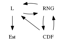
Figure 1: A diagram of the listed means of filling in one element of a model with another.

For most of these directions (${\textsc{L}}\to{\textsc{Est}}$, ${\textsc{RNG}}\to{\textsc{L}}$, ${\textsc{RNG}}\to{\textsc{CDF}}$), the ML-consistency requirements are met almost trivially; for the ${\textsc{L}}\to{\textsc{RNG}}$ and ${\textsc{CDF}}\to{\textsc{RNG}}$ algorithms, see the given citations for discussion of how the algorithms generate an RNG that is ML-consistent with the input likelihood and CDF.

Fiture 1 shows the directions presented here, clarifying that one can begin with any of L, RNG, or CDF and arrive at any of the four function elements of the model collection. The Est element is lossy, in the sense that one Est function ignores a great deal about the L function away from the optimum, and so may be equivalent to a variety of L functions.

Example 5: A network-generation simulation

This network generation simulation is based on agents with a position in an underlying preference space (in this case, ${\mathbb{R}}$). Each agent’s preferences are first generated as a draw from a ${\cal N}(0,1)$ distribution (though $\sigma$ will be allowed to vary in a variant below). Given two agents at positions $p_{i}$ and $p_{j}$, they link with probability $1/(1+|p_{i}-p_{j}|)$. The output is a list of how many links agents $1,\dots,N$ each have. It is useful to report sorted output, so the first dimension is the highest link count, down to the final dimension reporting the lowest link count. See Figure 2 for a summary of the algorithm.

 

1. Fix $\sigma=1$.

2. For each agent $i$:

   1. Draw a position $p_{i}$ using ${\textsc{RNG}}_{\cal N}(0,\sigma)$.

3. For each pair of agents, $i$ and $j$:

   1. Draw a random value $r\sim{\cal U}[0,1]$.

   2. Link iff $r\leq\frac{1}{1+|p_{i}-p_{j}|}$.

4. Output data $\leftarrow$ sorted count of connections for each person.

 

Figure 2: A simulation to produce a random distribution of link densities.

With $N=10$, one run of the simulation produces output in ${\mathbb{N}}^{10}$. Figure 3 plots the first two dimensions of the result of of 10,000 runs. For visualization purposes, a small jitter was added to each point.

The algorithm defines a model on ${\mathbb{P}}=\emptyset$ and ${\mathbb{D}}={\mathbb{N}}^{10}$. We have only defined the RNG portion of the model, but the above transformations indicate that the likelihood and other elements of the model can be well-defined by using the RNG.

Consider the hypothesis that the number of links to the most popular person is less than or equal to four. The number of links for the second, third, …persons are unrestricted, which we could express as the vacuous restriction that these link counts are less than or equal to nine. One would evaluate this hypothesis using the percentage of the total distribution that is below the point $[4,9,9,\dots,9]$, which is

$$CDF_{\rm sim}([4,9,9,\dots,9],\emptyset)\approx 0.0533.$$

Figure 3: A distribution of the number of links to the two highest-ranked members of a ten-person network. Plot produced by running the simulation in Figure 2, then adding a jitter to each point.

Examples 13 and 14 in the appendix present some uses of more elaborate simulation models.

4 Operations on models

This section presents a series of morphisms with signatures $f:{\mathbb{M}}\to{\mathbb{M}}$ or $f:({\mathbb{M}},{\mathbb{M}})\to{\mathbb{M}}$, that apply a well-defined transformation to every element of the input model(s) to produce a new model, including transformations via differentiable functions, fixing a parameter, or forming the product of independent distributions.

The transformations map to ${\mathbb{M}}$, so successive transformations can be chained together. As the examples below will demonstrate, the transformation paradigm allows models of arbitrary complexity to be built using simple steps.

4.1 Conditional results

But before writing down these transformations, a few things can be said about when two related models have equivalent elements, which will be useful in checking that our transformations are ML-consistent and related the way their descriptions claim they are.

The likelihood of ${\bf p}$

These statements will rely on an additional set of definitions:

defnLofP

$$L({\bf p})\equiv\int_{\forall\delta\in{\mathbb{D}}}L(\delta,{\bf p})d\delta$$

and

$$L({\bf d}|{\bf p})\equiv L({\bf d},{\bf p})/L({\bf p}).$$

The unitary axiom requires that $L({\bf p})\equiv 1,\forall{\bf p}$; dropping that assumption motivates the need for this definition. Recall that the definition of ML-consistency requires that $\infty>L({\bf p})>0$ for all ${\bf p}\in{\mathbb{P}}$.

defnLofD

$$L({\bf d})\equiv\int_{\forall\rho\in{\mathbb{P}}}L({\bf d},\rho)d\rho$$

and if $\infty>L({\bf d})>0$,

$$L({\bf p}|{\bf d})\equiv L({\bf d},{\bf p})/L({\bf d}).$$

This definition requires integrability on ${\mathbb{P}}$.

Equivalent elements

These definitions allow us to state when two models share Est, RNG, or CDF elements.

lmapreestinvar If for each ${\bf d}\in{\mathbb{D}}$ there exists a constant $K_{\bf d}$ such that

$${{\textsc{L}}_{2}({\bf d},{\bf p})}=K_{\bf d}{{\textsc{L}}_{1}({\bf d},{\bf p})},\forall{\bf p}\in{\mathbb{P}},$$

then ${\textsc{Est}}_{2}({\bf d})={\textsc{Est}}_{1}({\bf d})$.

This is sufficient but not necessary.

preestinvar For an arbitrary ${\bf d}\in{\mathbb{D}}$, ${\bf p}_{max}\equiv{\textsc{Est}}_{1}({\bf d})$ and any other ${\bf p}_{x}$,

$$L_{1}({\bf d},{\bf p}_{max}) \geq L_{1}({\bf d},{\bf p}_{x})\hbox{, so }$$

$$K_{\bf d}\cdot L_{1}({\bf d},{\bf p}_{max}) \geq K_{\bf d}\cdot L_{1}({\bf d},{\bf p}_{x})\hbox{, so }$$

$$L_{2}({\bf d},{\bf p}_{max}) \geq L_{2}({\bf d},{\bf p}_{x}).$$

Thus, ${\bf p}_{max}$ is also the argmax for $L_{2}({\bf d},\cdot)$, so ${\textsc{Est}}_{1}({\bf d})={\textsc{Est}}_{2}({\bf d})$. The premise of the lemma states that this holds for all ${\bf d}\in{\mathbb{D}}$.

propestinvariance If for each ${\bf d}\in{\mathbb{D}}$ there exists a constant $K_{\bf d}$ such that

$${{\textsc{L}}_{1}({\bf p}|{\bf d})}=K_{d}{{\textsc{L}}_{2}({\bf p}|{\bf d})},\forall{\bf p}\in{\mathbb{P}},$$

then ${\textsc{Est}}_{1}({\bf d})={\textsc{Est}}_{2}({\bf d})$.

estinvariance Because $L_{1}({\bf d})/L_{2}({\bf d})$ is constant for any given ${\bf d}$, $\frac{L_{1}({\bf d},{\bf p})}{L_{2}({\bf d},{\bf p})}$ is a constant iff $\frac{L_{1}({\bf p}|{\bf d})}{L_{2}({\bf p}|{\bf d})}$ is a constant; then preestinvar applies.

lmaprernginvar For each ${\bf p}\in{\mathbb{P}}$ there exists a constant $K_{\bf p}$ such that

$${{\textsc{L}}_{1}({\bf d},{\bf p})}=K_{\bf p}{{\textsc{L}}_{2}({\bf d},{\bf p})},\forall{\bf d}\in{\mathbb{D}}$$

iff ${\textsc{RNG}}_{1}({\bf p})={\textsc{RNG}}_{2}({\bf p})$ and ${\textsc{CDF}}_{1}({\bf p})={\textsc{CDF}}_{2}({\bf p})$.

prernginvar Given that $L_{1}({\bf d},{\bf p})=K_{\bf p}L_{2}({\bf d},{\bf p})$. By the definition of RNG (${\bf p}$), the ratio of the probability of drawing ${\bf d}_{1}$ to the probability of drawing ${\bf d}_{2}$ equals $\frac{L_{1}({\bf d}_{1},{\bf p})}{L_{1}({\bf d}_{2},{\bf p})},$ and this ratio does not change when we multiply the numerator and denominator by $K_{\bf p}$. The CDF element of the model is defined in terms of the RNG element.

In the other direction, ${\textsc{RNG}}_{1}({\bf p})={\textsc{RNG}}_{2}({\bf p})$ for some ${\bf p}$ implies that, for any arbitrary ${\bf d}_{1}$ and ${\bf d}_{2}$,

$$\frac{{\textsc{L}}_{1}({\bf d}_{1},{\bf p})}{{\textsc{L}}_{1}({\bf d}_{2},{\bf p})}=\frac{{\textsc{L}}_{2}({\bf d}_{1},{\bf p})}{{\textsc{L}}_{2}({\bf d}_{2},{\bf p})},$$

so

$$\frac{{\textsc{L}}_{1}({\bf d}_{1},{\bf p})}{{\textsc{L}}_{2}({\bf d}_{1},{\bf p})}=\frac{{\textsc{L}}_{1}({\bf d}_{2},{\bf p})}{{\textsc{L}}_{2}({\bf d}_{2},{\bf p})}\equiv K_{\bf p}.$$

proprnginvariance For each ${\bf p}\in{\mathbb{P}}$ there exists a constant $K_{\bf p}$ such that

$${{\textsc{L}}_{1}({\bf d}|{\bf p})}=K_{\bf p}{{\textsc{L}}_{2}({\bf d}|{\bf p})},\forall{\bf d}\in{\mathbb{D}}$$

iff ${\textsc{RNG}}_{1}({\bf p})={\textsc{RNG}}_{2}({\bf p})$ and ${\textsc{CDF}}_{1}({\bf p})={\textsc{CDF}}_{2}({\bf p})$.

rnginvariance $L_{1}({\bf p})/L_{2}({\bf p})$ is constant for a given ${\bf p}$. Then $\frac{{\textsc{L}}_{1}({\bf d}|{\bf p})}{{\textsc{L}}_{2}({\bf d}|{\bf p})}$ is constant iff $\frac{{\textsc{L}}_{1}({\bf d},{\bf p})}{{\textsc{L}}_{2}({\bf d},{\bf p})}$ is constant; then prernginvar applies.

The two propositions have a nice symmetry: proportional shifts in ${\textsc{L}}({\bf p}|{\bf d})$ do not affect Est; proportional shifts in ${\textsc{L}}({\bf d}|{\bf p})$ (which may differ from ${\textsc{L}}({\bf d},{\bf p})$ because we dropped the unitary axiom) do not affect RNG or CDF.

4.2 Parameter fixing

The simplest means of reducing an $N$-parameter model to an $N-1$-parameter model is to fix a parameter at a constant value, such as turning a two-parameter Normal distribution, ${\cal N}(\mu,\sigma)$, into a one-parameter distribution, ${\cal N}(\mu,1)$. One may also write this as ${\cal N}(\mu|\sigma=1)$.

Fix: $({\mathbb{M}},{\bf p}_{f}\in\underline{\mathbb{P}})\to{\mathbb{M}}$ $\blacktriangleright$ ${\mathbb{D}}^{\prime}={\mathbb{D}}$. $\blacktriangleright$ ${\mathbb{P}}^{\prime}=\underline{\mathbb{P}}^{\prime}$. $\blacktriangleright$ ${\textsc{L}}^{\prime}({\bf d},{\bf p}^{\prime})={\textsc{L}}({\bf d},{\bf p}_{f}\times{\bf p}^{\prime})$. $\blacktriangleright$ ${\textsc{Est}}^{\prime}$: use default of MLE. $\blacktriangleright$ ${\textsc{RNG}}^{\prime}({\bf p}^{\prime})={\textsc{RNG}}({\bf p}_{f}\times{\bf p}^{\prime})$. $\blacktriangleright$ ${\textsc{CDF}}^{\prime}({\bf p}^{\prime})={\textsc{CDF}}({\bf p}_{f}\times{\bf p}^{\prime})$.

Figure 4: Definition of the Fix mapping.

Figure 4 shows the mapping from input model and constraint to constrained output model. The mapping ${\mathbb{M}}\to{\mathbb{M}}$ breaks down into a mapping of the separate components of a model: parameter space to parameter space, likelihood function to likelihood function, and so on. The elements of the post-transform model are given a prime, such as ${\textsc{L}}^{\prime}(\cdot,\cdot)$, ${\textsc{Est}}^{\prime}(\cdot)$, ….

Some of these transformations require additional information to be fully described, which will be specified using subscripts. For example, a Normal model with $\sigma$ fixed at one will be written as ${\textsc{Fix}}_{\sigma=1}(M_{\cal N})$. These additional details are “private” to the generated model, used for the inner workings of the associated functions, but not used outside of the confines of the model.

Let the parameter subset be fixed at ${\bf p}_{f}\in\underline{\mathbb{P}}$, and the complement of its space in ${\mathbb{P}}$ be $\underline{\mathbb{P}}^{\prime}$, so $\underline{\mathbb{P}}\times\underline{\mathbb{P}}^{\prime}={\mathbb{P}}$. Elements in ${\mathbb{P}}^{\prime}$ are notated as ${\bf p}^{\prime}$. Then Figure 4 defines the Fix transformation.

The RNG and CDF equivalences are by rnginvariance. Because this general case offers no relation between ${\textsc{L}}({\bf p}|{\bf d})$ and ${\textsc{L}}^{\prime}({\bf p}^{\prime}|{\bf d},{\bf p}_{f})$, we are unable to reuse Est, although there are many well-known special cases.

4.3 Cross product

In an example below, we will want a prior for the $\mu$ and $\sigma$ of a Normal distribution. We could set the prior for $\mu$ as a Normal model and the prior for $\sigma$ as a square-root-transformed $\chi^{2}$ model (see differentiable transformations, below). These could be used sequentially, first setting $\sigma$ and then setting $\mu$, or this transformation could be used to bind together the two models to produce a model for $(\mu,\sigma)$.

Cross: ${\mathbb{M}}^{2}\to{\mathbb{M}}$ $\blacktriangleright$ ${\mathbb{D}}^{\prime}={\mathbb{D}}_{1}\times{\mathbb{D}}_{2}$. $\blacktriangleright$ ${\mathbb{P}}^{\prime}={\mathbb{P}}_{1}\times{\mathbb{P}}_{2}$ $\blacktriangleright$ ${\textsc{L}}^{\prime}({\bf d}^{\prime},{\bf p}^{\prime})={\textsc{L}}_{1}({\bf d}_{1},{\bf p}_{1})\cdot{\textsc{L}}_{2}({\bf d}_{2},{\bf p}_{2})$. $\blacktriangleright$ ${\textsc{Est}}^{\prime}=\left({\textsc{Est}}({\bf d}_{1}),{\textsc{Est}}({\bf d}_{2})\right)$ $\blacktriangleright$ ${\textsc{RNG}}^{\prime}=({\textsc{RNG}}_{1}({\bf p}_{1}),{\textsc{RNG}}_{2}({\bf p}_{2}))$. $\blacktriangleright$ ${\textsc{CDF}}^{\prime}={\textsc{CDF}}_{1}({\bf p}_{1})\cdot{\textsc{CDF}}_{2}({\bf p}_{2})$

Figure 5: Definition of the Cross mapping.

The simplest case of binding together two models is where both have distinct parameter spaces and data spaces. There is therefore effectively no interaction between the models, and the independence assumption dictates that ${\textsc{L}}^{\prime}({\bf d}^{\prime},{\bf p}^{\prime})={\textsc{L}}_{1}({\bf d}_{1},{\bf p}_{1})\cdot{\textsc{L}}_{2}({\bf d}_{2},{\bf p}_{2})$. Figure 5 specifies the rest of the Cross transformation.

The Cross morphism is associative, e.g.,

$${\textsc{Cross}}(M_{1},{\textsc{Cross}}(M_{2},M_{3}))={\textsc{Cross}}({\textsc{Cross}}(M_{1},M_{2}),M_{3}).$$

Therefore, there is no ambiguity in writing ${\textsc{Cross}}(M_{1},M_{2},M_{3})$ to represent the combination of three models.

Mix: $({\mathbb{M}}^{2},w\in[0,1])\to{\mathbb{M}}$ $\blacktriangleright$ ${\mathbb{D}}^{\prime}={\mathbb{D}}_{1}={\mathbb{D}}_{2}$ $\blacktriangleright$ ${\mathbb{P}}^{\prime}={\mathbb{P}}_{1}\times{\mathbb{P}}_{2}\times[0,1]$ $\blacktriangleright$ $L_{M}({\bf d},{\bf p}_{M})=wL_{1}({\bf d},{\bf p}_{1})+(1-w)L_{2}({\bf d},{\bf p}_{2}).$ $\blacktriangleright$ ${\textsc{Est}}^{\prime}$: Typically solved via EM algorithm (Dempster et al., 1977). $\blacktriangleright$ ${\textsc{RNG}}^{\prime}$: First, draw a random number $r\sim{\cal U}[0,1]$. $${\textsc{RNG}}^{\prime}(p_{M})=\left\{\begin{array}[]{ll}{\textsc{RNG}}_{1}({\bf p}_{1})&r\leq w\\ {\textsc{RNG}}_{2}({\bf p}_{2})&r>w\end{array}\right.$$ $\blacktriangleright$ ${\textsc{CDF}}^{\prime}({\bf p}_{w})=w{\textsc{CDF}}_{1}({\bf d},{\bf p}_{1})+(1-w){\textsc{CDF}}_{2}({\bf d},{\bf p}_{2})$.

Figure 6: Definition of the Mix mapping.

4.4 Model mixing

Consider two models, both over the same data space ${\mathbb{D}}$ but distinct parameter spaces ${\mathbb{P}}_{1}$ and ${\mathbb{P}}_{2}$, and a weighting $w\in[0,1]$, and let ${\mathbb{P}}_{M}$ be the Cartesian product ${\mathbb{P}}_{1}\times{\mathbb{P}}_{2}\times[0,1]$; in the other direction, one could decompose a point ${\bf p}_{m}$ into its three parts, ${\bf p}_{1}$, ${\bf p}_{2}$, and $w$. Figure 6 displays the Mix transformation mapping from two models and a weight to a model representing the mixture.

As per examples to follow, the mixture transformation is especially useful in combination with the Fix transformation, for the purposes of fixing just the weights (fixing $w\equiv 0.5$ is a popular choice), or fixing ${\bf p}_{1}$ and ${\bf p}_{2}$ and leaving the estimation only to find the most likely $w$.

As with Cross, one could recursively use the two-input Mix transformation to mix three or more models.

4.5 Data Constraint

Let the constraint function ${\rm Con}_{d}:{\mathbb{D}}\to\{0,1\}$ be an indicator function that is one when the input data is within some desired boundary and zero when it is not, and let the constrained data space ${\mathbb{D}}^{\prime}$ be the set of data points where ${\rm Con}_{d}({\bf d})=1$.

DataTrunc: $({\mathbb{M}},{\rm Con}_{d}:{\mathbb{D}}\to\{0,1\})\to{\mathbb{M}}$ $\blacktriangleright$ ${\mathbb{D}}^{\prime}=$ the subset of ${\mathbb{D}}$ where ${\rm Con}_{d}$ is one. $\blacktriangleright$ ${\mathbb{P}}^{\prime}={\mathbb{P}}.$ $\blacktriangleright$ ${\textsc{L}}^{\prime}({\bf d},{\bf p})=\frac{{\textsc{L}}({\bf d},{\bf p})}{\int_{{\mathbb{D}}^{\prime}}L(\delta,{\bf p})d\delta}$. $\blacktriangleright$ ${\textsc{Est}}^{\prime}$: use MLE. $\blacktriangleright$ ${\textsc{RNG}}^{\prime}$: Draw ${\bf d}$ using RNG. If ${\rm Con}_{d}({\bf d})=0$, throw ${\bf d}$ out and try again. $\blacktriangleright$ ${\textsc{CDF}}^{\prime}$: Random draws from ${\textsc{RNG}}^{\prime}$ can be used to calculate the CDF.

Figure 7: Definition of the DataTrunc mapping.

Figure 7 describes a transformation, DataTrunc, for the case where data outside the constraint is suppressed. See Cameron and Trivedi (1998, §4.5) for a discussion of how maximum likelihood estimation of ${\textsc{L}}_{{\textsc{DataTrunc}}}$ recovers the parameters of the unconstrained model, and Listing 17 for an example implementing and demonstrating the transformation.

rnginvariance shows that within ${\mathbb{D}}^{\prime}$, ${\textsc{RNG}}^{\prime}$ and ${\textsc{CDF}}^{\prime}$ must be identical to RNG and CDF; and it is easy to verify that ${\textsc{RNG}}^{\prime}$ is ML-consistent with ${\textsc{L}}^{\prime}$.

Because the scaling for L depends upon ${\bf p}$, for an arbitrary unconstrained model $M$, ${\textsc{L}}_{{\textsc{DataTrunc}}(M)}({\bf p}|{\bf d})/{\textsc{L}}_{M}({\bf p}|{\bf d})$ is not constant over all ${\bf p}$, so estinvariance does not apply and the Est routines will differ between pre- and post-transformation models.

Example 6: A censored distribution with a point mass

One could write the case of a truncated Normal distribution where any ${\bf d}<0$ is discarded using $M_{\rm trunc}={\textsc{DataTrunc}}_{x\geq 0}(M_{\cal N})$.

But consider a $M_{\cal N}$ with all observations less than zero reported as exactly zero. One could use the models and transformation to this point to begin to express this model, which is the combination of a PMF based on one data point and a truncated Normal.

$$M_{F} = {\textsc{Fix}}_{(w=1,{\bf d}=0)}(M_{PMF})$$

$$M_{T} = {\textsc{DataTrunc}}_{{\bf d}\geq 0}(M_{\cal N}).$$

Mixcdf: ${\mathbb{M}}^{2}\to{\mathbb{M}}$ $\blacktriangleright$ ${\mathbb{D}}^{\prime}={\mathbb{D}}_{1}={\mathbb{D}}_{2}$ $\blacktriangleright$ ${\mathbb{P}}^{\prime}={\mathbb{P}}_{1}\times{\mathbb{P}}_{2}$ $\blacktriangleright$ ${\textsc{L}}^{\prime}({\bf d},{\bf p}_{M})={\textsc{CDF}}_{\cal N}(0)\cdot L_{1}({\bf d},{\bf p}_{1})+(1-{\textsc{CDF}}_{\cal N}(0))L_{2}({\bf d},{\bf p}_{2}).$ $\blacktriangleright$ ${\textsc{Est}}^{\prime}$: use default of MLE. $\blacktriangleright$ ${\textsc{RNG}}^{\prime}$, ${\textsc{CDF}}^{\prime}$: as per ${\textsc{Fix}}_{w={\textsc{CDF}}_{\cal N}(0)}({\textsc{Mix}}(M_{T},M_{F}))$ (by rnginvariance).

Figure 8: Definition of the Mixcdf mapping.

It is not quite correct to say that the final model is a mixture of $M_{F}$ and $M_{T}$, because the mixing weight for ${\textsc{Mix}}(M_{F},M_{T})$ needs to be ${\textsc{CDF}}(0,M_{\cal N})$, which is itself a function of $\mu$ and $\sigma$. We do not yet have a transformation that sets a parameter at the value of a CDF, but it is trivial to write an ad hoc transformation for the situation; see Figure 8 for a description of the Mixcdf transformation.

Then the final model of a ${\cal N}(\mu,\sigma)$ with values less than zero replaced to zero is $M_{\rm Ncut}\equiv\textsc{Mixcdf}(M_{T},M_{F})$.

Jacobian: $({\mathbb{M}},f:{\mathbb{R}}^{N}\to{\mathbb{R}}^{N})\to{\mathbb{M}}$ $\blacktriangleright$ ${\mathbb{D}}^{\prime}={\mathbb{D}}={\mathbb{R}}^{N}$. $\blacktriangleright$ ${\mathbb{P}}^{\prime}={\mathbb{P}}$. $\blacktriangleright$ ${\textsc{L}}^{\prime}({\bf d},{\bf p})={\textsc{L}}(f^{-1}({\bf d}),{\bf p})|\det(J(f^{-1})({\bf d}))|$. $\blacktriangleright$ ${\textsc{Est}}^{\prime}={\textsc{Est}}(f^{-1}({\bf d}))$ $\blacktriangleright$ ${\textsc{RNG}}^{\prime}=f({\textsc{RNG}}({\bf p}))$ $\blacktriangleright$ ${\textsc{CDF}}^{\prime}$: Use default.

Figure 9: Definition of the Jacobian mapping.

4.6 Differentiable transformation

Consider a transformation function $f:{\mathbb{R}}^{N}\to{\mathbb{R}}^{N}$, with inverse $f^{-1}:{\mathbb{R}}^{N}\to{\mathbb{R}}^{N}$, and inverse derivative matrix (the Jacobian) $J(f^{-1})$. The likelihood in the mapped-to space is the likelihood in the original space weighted by $|\det(J(f^{-1}))|$ See, for example, Greene (1990). The transformation of likelihoods can naturally be extended to a transformation of full models, as per Figure 9.

The set of invertible functions over a given space ${\mathbb{D}}$ under the function composition operator forms a group. Therefore, for a given base model $M_{b}$, the set of models ${\textsc{Jacobian}}_{f}(M_{b})$ over the same set of functions also form a group under the model composition function defined by ${\textsc{Jacobian}}_{f}(M_{b})\circ{\textsc{Jacobian}}_{g}(M_{b})\equiv{\textsc{Jacobian}}_{f\circ g}(M_{b})$.

Further, by the Radon–Nikodym theorem, for any two absolutely continuous models with respect to a given measure, there exists a transformation between them. Thus, some applications of other transformations in this paper are special cases of the Jacobian transformation.

Example 7: Volume

If the lengths of a set of cubes has a truncated-at-zero Normal distribution, ${\textsc{DataTrunc}}_{{\bf d}>0}(M_{\cal N})$, then the volumes are described by

$$M_{\rm cube}={\textsc{Jacobian}}_{f(x)=x^{3}}({\textsc{DataTrunc}}_{{\bf d}>0}(M_{\cal N})).$$

Swap: ${\mathbb{M}}\to{\mathbb{M}}$ $\blacktriangleright$ ${\mathbb{D}}^{\prime}={\mathbb{P}}$ $\blacktriangleright$ ${\mathbb{P}}^{\prime}={\mathbb{D}}$ $\blacktriangleright$ ${\textsc{L}}^{\prime}({\bf d}^{\prime},{\bf p}^{\prime})={\textsc{L}}({\bf p}^{\prime},{\bf d}^{\prime})$. $\blacktriangleright$ ${\textsc{Est}}^{\prime},{\textsc{RNG}}^{\prime},{\textsc{CDF}}^{\prime}$: use defaults.

Figure 10: Definition of the Swap mapping.

4.7 Swapping parameters and data

Because data and parameters are not symmetric in the definition of a model, swapping them produces a new model, as per the Swap transformation defined in Figure 10. Notably, the estimation process searches for the most likely parameters given fixed data, so the post-swap model’s estimation searches the orignal model’s data space given a fixed value in the original model’s parameter space.

This will be used in Section 4.8.2 to implement random draws from a data space via Markov Chain Monte Carlo and Section 5.1 for finding the most likely prediction from a model.

4.8 Composition

The transformations in this section consist of chaining together the output from one model ($M_{\rm from}$) as input to the next ($M_{\rm to}$). Given that each model is associated with two spaces, there are four possible means of chaining output from the first model to input to the second.

• If ${\mathbb{D}}_{\rm from}$ is generated from the RNG of the first model, linking ${\mathbb{D}}_{\rm from}={\mathbb{D}}_{\rm to}$, allows us to evaluate the draws of one model using the likelihood and estimation routines of another model.

• In a hierarchical model, the parameter estimate from the child model(s) is used as a data set for the parent model, in the form ${\mathbb{P}}_{\rm from}={\mathbb{D}}_{\rm to}$.

• Matching ${\mathbb{D}}_{\rm from}={\mathbb{P}}_{\rm to}$ produces what is commonly referred to as Bayesian updating.

• The pairing ${\mathbb{P}}_{\rm from}={\mathbb{P}}_{\rm to}$ is of limited utility.

4.8.1 Data composition (${\mathbb{D}}_{\rm from}={\mathbb{D}}_{\rm to}$)

The direction of ${\mathbb{D}}_{\rm from}={\mathbb{D}}_{\rm to}$ is most commonly implemented by using random draws from the first model as the input data set for the second. Let $Nseq\in{\mathbb{N}}^{N}$ be an arbitrary sequence of natural numbers (in practice, draws from a PRNG). Then ${\textsc{RNG}}_{\rm to}({\bf d}_{\rm to})\in{\mathbb{D}}_{\rm to}$, and because ${\mathbb{D}}_{\rm from}={\mathbb{D}}_{\rm to}$, the draw can be used as an input to ${\textsc{L}}_{\rm from}$. Figure 11 details the rest of this composition.

Dcompose: $({\mathbb{M}}^{2},Nseq\in{\mathbb{N}}^{N})\to{\mathbb{M}}$ $\blacktriangleright$ ${\mathbb{D}}^{\prime}=\emptyset$. $\blacktriangleright$ ${\mathbb{P}}^{\prime}={\mathbb{P}}_{\rm to}\times{\mathbb{P}}_{\rm from}$. $\blacktriangleright$ ${\textsc{L}}^{\prime}(\emptyset,{\bf p})={\textsc{L}}_{\rm from}({\textsc{RNG}}_{\rm to}({\bf d}_{\rm to},{\bf p}_{\rm to},Nseq),{\bf p}_{\rm from})$. $\blacktriangleright$ ${\textsc{Est}}^{\prime}$: use default of MLE. $\blacktriangleright$ ${\textsc{RNG}}^{\prime}({\bf p})=\emptyset$. $\blacktriangleright$ ${\textsc{CDF}}^{\prime}=\emptyset$.

Figure 11: Definition of the Dcompose mapping.

Attaching a fixed sequence of draws to the model retains the model structure: the likelihood is deterministic and does not require additional PRNG inputs, and similarly for the estimation routine. Each sequence $Nseq$ therefore defines a new model. In practice, the class of models would likely be implemented on the fly, with random draws made as needed. In such a case, L and the MLE that depends on L are stochastic. Some ML search methods are better suited to stochastic search (e.g., simulated annealing, simplex algorithms) than others (e.g., conjugate gradient searches).

Example 8: Exponentially-distributed random graphs

Distributions of network link counts in human networks are known to take a few known distributions, including the Exponential, Waring, Yule, or Zipf distributions.

So it is sensible to evaluate how well the simulated networks produced by the network generation model above, $M_{Sim}$, fit to an Exponential distribution, $M_{Exp}$.

The network generation model produces data appropriate for composing with the Exponential distribution. The composed model,

$$M_{\rm Ncomp}={\textsc{Dcompose}}_{Nseq}(M_{Sim},M_{Exp}),$$

has ${\mathbb{D}}=\emptyset$ and ${\mathbb{P}}={\mathbb{R}}$, and can be used to evaluate the likelihood of the network link counts generated by $M_{Sim}$ using the likelihood function of an Exponential distribution.

In the specification of Example 5, $\sigma$ was fixed at one, and so ${\mathbb{P}}_{Sim}=\emptyset$; consider the variant $M_{\sigma Sim}$ where $\sigma$ is not fixed, so ${\mathbb{P}}_{\sigma Sim}=\sigma$, and $M_{Sim}$ = ${\textsc{Fix}}_{\sigma=1}(M_{\sigma Sim})$. What is the simulation that comes closest to an Exponential model with $\lambda=1$? We could answer this question by writing down the model $M_{fix\lambda}={\textsc{Fix}}_{\lambda=1}(M_{\sigma Sim},M_{Exp})$, and using its estimate routine to find the optimal parameter $\sigma_{\rm opt}={\textsc{Est}}_{fix\lambda}$. Evaluating ${\textsc{Est}}_{fix\lambda}$ gives $\sigma\approx 0.51$.

4.8.2 Parameter composition (${\mathbb{D}}_{\rm from}={\mathbb{P}}_{\rm to}$)

This form of composition is generally referred to by its immediate application: Bayesian updating.

For example, let $M_{likelihood}={\textsc{Fix}}_{\sigma=1}(M_{\cal N})$ (so ${\mathbb{P}}_{\rm likelihood}={\mathbb{R}}$, representing $\mu$), and let a Normal distribution with known $\mu$ and $\sigma$ be the prior model (so ${\mathbb{D}}_{\rm prior}={\mathbb{R}}$). Then the data space of the prior matches the parameter space of the likelihood. There are several ways to implement the elements of this model, discussed below.

More generally, let $M_{\rm prior}$ have $\rho\in{\mathbb{P}}_{\rm prior}$ and ${\bf p}\in{\mathbb{D}}_{\rm prior}$, and $M_{\rm likelihood}$ have ${\bf d}\in{\mathbb{D}}_{\rm likelihood}$ and ${\bf p}\in{\mathbb{P}}_{\rm likelihood}$. The calculation of ${\textsc{L}}_{\rm posterior}({\bf p}|\rho,{\bf d})$ can be broken down via Bayes’s rule to be proportional to:

$${\textsc{L}}_{\rm prior}({\bf p}|\rho)\cdot{\textsc{L}}_{\rm likelihood}({\bf d}|{\bf p}.\rho),$$ (1)

DPcompose: $({\mathbb{M}}^{2},\rho\in{\mathbb{P}}_{\rm prior})\to{\mathbb{M}}$ $\blacktriangleright$ ${\mathbb{D}}^{\prime}={\mathbb{D}}_{\rm like}$ $\blacktriangleright$ ${\mathbb{P}}^{\prime}={\mathbb{D}}_{\rm prior}$ $\blacktriangleright$ ${\textsc{L}}^{\prime}=L_{\rm prior}({\bf p},\rho){\textsc{L}}_{\rm like}({\bf d}|{\bf p})$ $\blacktriangleright$ ${\textsc{Est}}^{\prime}$: table of conjugates, rejection sampling, or MLE. $\blacktriangleright$ ${\textsc{RNG}}^{\prime},{\textsc{CDF}}^{\prime}$: posterior draw, Metropolis-Hastings or draw from prior.

Figure 12: Definition of the DPcompose mapping.

We take $\rho\in{\mathbb{P}}_{\rm prior}$ as a fixed-with-certainty prior belief regarding the parameters of the prior model, ${\bf d}$ as being observed with certainty, and use the fact that L need not integrate to one to specify the likelihood of the posterior model. Figure 12 details this data-parameter composition transformation in full.

The default/model-specific set for estimating this transformation has three parts.

Conjugate priors

Some pairs of models are conjugate distributions, which have known, closed-form posteriors. Tables of conjugate pairs are readily available. In this case, the Est, RNG, L, and CDF elements of the prior-likelihood composition can be replaced with the corresponding elements of the posterior model.

Likelihood prior

Metropolis-Hastings Markov chain Monte Carlo (MHMCMC) can be used to draw from a distribution where the likelihood function can be easily calculated to within some constant proportion, as in the case of Equation 1. We could thus use it to make random draws from a prior-likelihood pair. See Metropolis et al. (1953) for details of the algorithm, which will be notated here as a function $Metro:({\mathbb{M}},{\mathbb{M}})\to{\mathbb{P}}$. Given this function, one can implement Bayesian updating using the tools described to this point.

• Generate a model whose likelihood is the product of the input likelihoods via $M_{c}$ = DPcompose ($M_{prior}$, $M_{likelihood}$).

• MHMCMC makes draws from the parameter space given fixed data, but we want to make draws from data space given fixed parameters, so generate $M_{sc}$ =Swap ($M_{c}$).

• MHMCMC requires a proposal distribution. A Normal distribution is a popular choice, so let $M_{propose}=M_{\cal N}$.

• $Metro$ draws from the proposal and accepts or rejects the draw using a target distribution, so we have enough to generate an RNG for the model, drawing from the data space of $M_{propose}$ and testing it against $M_{sc}$.

Figure 13 is a diagram depicting the setup, a model where

$${\textsc{RNG}}_{post}=Metro(M_{\cal N},{\textsc{Swap}}({\textsc{DPcompose}}(M_{prior},M_{like}))).$$

1pt

Posterior model RNG: Metro(proposal, target) proposal: ${\cal N}$ target: Swap $L(d,{\bf p})\equiv L_{DPcompose}({\bf p},{\bf d})$ DPcompose $L({\bf d},{\bf p})=L_{pri}({\bf p},{\bf p}^{\prime})\cdot L_{like}({\bf d}|{\bf p})$ Prior $L_{prior}:{\mathbb{D}},{\mathbb{P}}\to{\mathbb{R}}^{+}_{0}$ Likelihood $L_{like}:{\mathbb{D}},{\mathbb{P}}\to{\mathbb{R}}^{+}_{0}$

Figure 13: A posterior distribution augmented with an RNG element based on Metropolis-Hastings MCMC. Each box is a model; many transform the models embedded within their box.

RNG prior

Consider a prior that has no explicit L element, but does have an RNG element. We will build a PMF model for the posterior which, as above, has a parameter set consisting of a list of pairs $(w_{i},{\bf p}_{i})$. For a fixed prior parameter $\rho$, make a draw of ${\bf p}_{i}$ from the prior; by definition, this has likelihood proportional to ${\textsc{L}}_{\rm prior}({\bf p}_{i},\rho)$. Let $M_{\rm fm}({\bf d},{\bf p})={\textsc{Fix}}_{{\bf p}}(M_{\rm like})$ and set the weight for this datum as $w_{i}={\textsc{L}}_{\rm fm}({\bf d}|{\bf p}_{i})$. Then, as the count of elements $\to\infty$, a draw from the PMF $(w_{i},{\bf p}_{i})$ is proportional to ${\textsc{L}}^{\prime}={\textsc{L}}_{\rm fm}({\bf d}|{\bf p}_{i})d{\textsc{L}}_{\rm prior}({\bf p}_{i},\rho)$.

MCMC methods are popular in part because the proposal distribution ‘walks around’ in the target distribution, spending more time in the regions with greater weight, so a mismatched proposal (like a ${\cal N}(0,1)$ proposal for a ${\cal N}(5,1)$ target) will adapt to become a well-matched proposal. Conversely the fixed prior model does not move, and always makes more draws from the region(s) of the prior model with the most weight. This can be inefficient if there is a large mismatch between the prior and the likelihood. As the number of draws goes to infinity, drawing from the prior directly and drawing from a proposal distribution would be equivalent, but for a small number of draws, the MCMC chain generally gives smoother results. However, the direct-draw method is feasible for RNG-based models for which MCMC is not, and is not sequential. Typical computers in the present day can run several threads in parallel (thousands at once in an increasing number of cases), and there may exist conditions where a larger volume of parallel stationary draws could generate a more accurate posterior than the adaptive sequential method.

Example 9: Bayesian updating with a simulation

Example 8 built $M_{Ncomp}$ to describe a network simulation where the likelihood of a set of randomly generated networks was described via an Exponential distribution.

We may have prior beliefs that $\lambda\sim{\textsc{Fix}}_{(\mu=m,\sigma=s)}(M_{\cal N})$ for some known parameters $(\mu=m,\sigma=s)$. Then we can generate a new model as

$$M_{\rm post1}={\textsc{DPcompose}}({\textsc{Fix}}_{(\mu=m,\sigma=s)}(M_{\cal N}),M_{Ncomp}).$$

Figure 14 shows the PMF reduction of this model.

Some authors draw a dichotomy between models that are on the table of conjugate distributions, and can therefore be treated parametrically, and all other models whose posterior must be approximated by a nonparametric distribution. However, one can leave the model expressed using the prior’s ${\mathbb{P}}$ and the likelihood’s ${\mathbb{D}}$. Here,

$$M_{\rm post2}={\textsc{DPcompose}}(M_{\cal N},M_{Ncomp}),$$

has ${\mathbb{P}}={\mathbb{R}}\times{\mathbb{R}}^{+}_{0}$, representing $\mu$ and $\sigma$. It is a parametric model like any other, and its parameters can be estimated using ${\textsc{Est}}_{\rm post2}(\emptyset)$, and their confidence bounds can be calculated using (stochastically appropriate) methods from Section 5.2.

Figure 14: A PMF representing the posterior distribution of $\lambda$ in the ${\textsc{Dcompose}}_{Nseq}(M_{Net},M_{exp})$ model.

4.8.3 Hierarchical modeling (${\mathbb{P}}_{\rm child}={\mathbb{D}}_{\rm parent}$)

Consider a school, consisting of several classrooms. Each classroom provides a distinct data set $d_{1},\dots,d_{N}$, from which we can estimate the parameters of a model, such as a set of regression coefficients or characteristics of a network model. Stacking a model for each classroom produces $M_{\rm classes}=$ ${\textsc{Cross}}(M_{\rm class1},$ $\dots,$ $M_{\rm classN})$, where ${\textsc{Est}}_{\rm classes}({\bf d}_{1}\times\dots\times{\bf d}_{N})$ is a stack of parameters $({\textsc{Est}}({\bf d}_{1}),$ $\dots,$ ${\textsc{Est}}({\bf d}_{N}))$ that can then be used as a data set for a school-wide model.

PDcompose: ${\mathbb{M}}^{2}\to{\mathbb{M}}$ $\blacktriangleright$ ${\mathbb{D}}^{\prime}={\mathbb{D}}_{\rm child}$ $\blacktriangleright$ ${\mathbb{P}}^{\prime}={\mathbb{P}}_{\rm parent}$ $\blacktriangleright$ ${\textsc{L}}^{\prime}({\bf d},{\bf p})={\textsc{L}}_{\rm parent}({\textsc{Est}}_{\rm child}({\bf d}),{\bf p})$ $\blacktriangleright$ ${\textsc{Est}}^{\prime}({\bf d})={\textsc{Est}}_{\rm parent}({\textsc{Est}}_{\rm child}({\bf d}))$ $\blacktriangleright$ ${\textsc{RNG}}^{\prime}$: draw $\underline{{\bf p}}={\textsc{RNG}}_{\rm parent}({\bf p})$, then return ${\textsc{RNG}}_{\rm child}(\underline{{\bf p}})$. $\blacktriangleright$ ${\textsc{CDF}}^{\prime}$: use defaults

Figure 15: Definition of the PDcompose mapping.

It can be shown (Box and Tiao, 1992) that in the case of linear models for both parent and child, the model can be reduced to a single linear model. This is a special case of the general form, where the parent and child models could take any arbitrary form, so long as the parameter space of the child models match the data space of the parent model. Figure 15 describes this parameter-data composition transformation in detail.

Example 10: A narrative model

The format of transforming simple models to produce more complex models suggests and facilitates a style of narrative modeling, in which a real-world problem is broken down into basic components and the manner by which the components are hypothesized to combine is explicitly described via corresponding model transformations.

In this example, consider the arrival times of dinner party guests. One type of guest tries to be on time, but may face delays, which occur at the rate of $\lambda$ per minute. The second type of guest tries to be fashionably late, ideally arriving 30 minutes late, but hitting that mark imprecisely. Nobody is early: those who miscalculate and arrive in the neighborhood before the stated start time take care to delay enough to arrive exactly on time.

The likelihood function for an Exponential distribution describes the percent of a group not yet exited from a population given departures at a rate $\lambda$ as described above. The derivative of one minus ${\textsc{L}}_{\rm exp}$ therefore describes the arrival rate at any given point in time, and the reader can verify that this is

$$M_{A}={\textsc{Jacobian}}_{1/\lambda}(M_{\rm Exp}).$$

The second group is reasonably described by a Normal distribution, with values less than zero fixed to exactly zero. This is the $M_{\rm Ncut}$ model developed above. Assuming the two groups are evenly split, the overall group is

$$M_{\rm grp}={\textsc{Fix}}_{w=0.5}({\textsc{Mix}}({\textsc{Jacobian}}_{1/\lambda}(M_{\rm Exp}),M_{\rm Ncut})).$$

This model has ${\mathbb{D}}={\mathbb{R}}^{+}_{0}$, representing minutes late; and ${\mathbb{P}}={\mathbb{R}}^{+}_{0}\times{\mathbb{R}}\times{\mathbb{R}}^{+}$, for $(\lambda,\mu,\sigma)$.

We should put priors on these parameters. For $\lambda$, ${\textsc{DataTrunc}}_{x>0}(M_{\cal N})$ is a reasonable form for a prior; for $\mu$, we could use $M_{\cal N}$; for $\sigma$, we could use the square root of a $\chi^{2}$ model, ${\textsc{Jacobian}}_{\sqrt{x}}(M_{\chi^{2}})$ with parameters $\Sigma$. Then the prior is

$$M_{\rm pri}={\textsc{Cross}}({\textsc{DataTrunc}}_{x>0}(M_{\cal N}),M_{\cal N},{\textsc{Jacobian}}_{\sqrt{x}}(M_{\rm InvWish}))$$

The overall model is then $M={\textsc{DPcompose}}(M_{\rm pri},M_{\rm grp})$. It has parameters ${\mathbb{P}}$ representing $(\mu_{1},\sigma_{1},\mu_{2},\sigma_{2},\Sigma)$, and ${\mathbb{D}}={\mathbb{R}}^{+}_{0}$ representing minutes late.

There are a several things that one could do with $M$. One would be to fix the input parameters to reasonable prior beliefs, use rejection sampling to reduce $M$ to a nonparametric PMF, and compare the model to data using the data-space tests described in Section 5. Or, one could estimate the five input parameters via ${\textsc{Est}}(M)$ and run parameter-space tests (also discussed below) to give confidence bounds on the prior parameters.

5 Applications

This section lists a few existing methods that operate on generic black-box models. Any of the models described to this point could be used for any of these applications. This section assumes the reader is already familiar with the methods, and will only briefly discuss the considerations needed to construct algorithms around elements of ${\mathbb{M}}$, and their use for the broad range of models that this paper contemplates.

As with many of the elements to this point, the goal is to establish an implementation for all models; closed-form implementations for certain models can be filled in as needed.

Before discussing a few more notable functions in detail, here are a few calculations that can work with input of a generic model (or models) in a straightforward manner:

• Entropy.

• Kullback-Leibler divergence.

• Cook’s distance and other leave-$N$-out cross-validation techniques.

• Derivatives and second derivatives of differentiable parameters.

5.1 Prediction

The prediction problem is effectively a problem of partially missing data. For example, given the independent variables of an OLS model, ${\bf X}$, we may wish to predict the most likely values of the missing dependent variable ${\bf Y}$. We can generate a default algorithm for this problem using the tools above.

Given a model $M$ with known parameters ${\bf p}$, estimated using some reference or training data, ${\bf p}={\textsc{Est}}({\bf d}_{\rm ref})$, then ${\textsc{Swap}}(M)$ generates a model where the original ${\bf p}$ is treated as fixed data. ${\textsc{Est}}_{{\textsc{Swap}}(M)}({\bf p})$ produces the most likely data for $M$. Now consider a data set ${\bf D}$, divided into known and unknown parts, ${\bf D}_{\rm known}$ and ${\bf D}_{\rm miss}$. Then we can fix some parameters of ${\textsc{Swap}}(M)$ at ${\bf D}_{\rm known}$, leaving a model whose only unknown parameters are those in ${\bf D}_{\rm miss}$. Then the model is $M_{pred}={\textsc{Fix}}_{{\bf D}_{\rm known}}({\textsc{Swap}}(M))$, and the maximum likelihood estimate of the data elements to be predicted is ${\textsc{Est}}_{pred}({\bf p})$.

5.2 Testing

Given that models in ${\mathbb{M}}$ are an intermediary between a data space and a parameter space, it makes sense to divide tests into those regarding the data space and those regarding the parameter space.

5.2.1 Parameter-space tests

A test about a claim regarding the parameters has three steps:

1. Specify a statistic, such as a parameter estimate.

2. State the distribution of the statistic estimate as specified by the model.

3. Find the odds that the statistic lies within some given range of interest using the CDF of the statistic as specified by the model.

For example, after an OLS regression, the assumptions of the model indicate that the parameter estimates are Multivariate Normal, and that fact is commonly used to state the likelihood with which each parameter differs from zero.

We have a model’s parameter estimates, from ${\textsc{Est}}(\cdot)$, but also need the distribution of the estimates. Setting aside those models (such as OLS) where it can be derived via closed-form calculations, there are a few default methods available.

Covariance via bootstrap and jackknife

These methods take in a data set and an estimation routine (Efron and Gong, 1983; Efron and Tibshirani, 1993). For iteration $i$ of the algorithm, both methods generate an artificial data set (the bootstrap, via sampling with replacement; the jackknife via a leave-$n$-out process), then run the estimation routine to calculate $\hat{}{\bf p}_{i}$. Once several hundred or thousand such parameter estimates are derived, the covariance matrix is calculated for the given parameters.

The final estimate of the statistic is the mean of the statistic calculated for each data subset, so central limit theorems typically apply. These techniques therefore apply to a wide range of models. However, they assume that draws from the data are analogous to draws from the true population.

Simple replication

For the network model in Examples 5, 8, and 9, where ${\mathbb{D}}=\emptyset$, the parameter distribution can be produced by repeated draws from the RNG. This is not bootstrapping, and does not rely on the core assumption of bootstrapping: in a sense, the draws from the RNG could be thought of as the true population asserted by the model.

Covariance via inverse Hessian

The Fisher Information matrix is the negation of the inverse of the expected Hessian matrix (the matrix of second derivatives of the log likelihood function). Especially for likelihood functions that are well-approximated by a Taylor expansion to the second (squared) degree, Fisher Information can be a good estimate of the parameter variance, and thus a good input to parametric hypothesis tests. Evaluating the quality of a second-degree Taylor approximation in the neighborhood of an MLE can also be done using only the model and a data set.

5.2.2 Data-space tests

For models where ${\mathbb{P}}$ is either trivial enough that it is $\emptyset$ or so complex that the dimensionality of a given element ${\bf p}\in{\mathbb{P}}$ is unknown (i.e., for nonparametric models), it is difficult to use parameter-space tests. In this case, we can develop metrics to describe the distance between models via computations over the data space.

One class of tests involve finding the distance from the fitted model to a target model constructed by producing a PMF from a set of observed data, distinct from the data used to estimate the model being tested. Given the two PMFs, there is then the problem of summarizing their differences in a single statistic.

There are many options, and it it is beyond the scope of this paper to describe their relative merits, but this segment discusses the problem of applying any of them to an arbitrary element of ${\mathbb{M}}$.

Recall that the parameters of a PMF are a set of weights associated with points in the data space: $\left((w_{1},{\bf d}_{1}),(w_{2},{\bf d}_{2}),\dots,(w_{N},{\bf d}_{N})\right)$. Given a second model that has different weights at the same data points—i.e., a model with parameters $\left((w_{1}^{\prime},{\bf d}_{1}),(w_{2}^{\prime},{\bf d}_{2}),\dots,(w_{N}^{\prime},{\bf d}_{N})\right)$—one could calculate the distance between the vector $(w_{1},\dots,w_{N})$ and $(w_{1}^{\prime},\dots,w_{N}^{\prime})$ by a number of means:

• $k$-fold cross-validation tools typically report normalized Euclidian distance, aka root mean squared error, between the predicted and observed PMFs.

• Kullback-Leibler divergence can be used to measure the information loss from the actual to the predicted observations.

• The Kolmogorov-Smirnov test reports a statistic based on the maximum distance between the CDFs of the two distributions.

Given a PMF and an arbitrary distribution also defined over the same ${\mathbb{D}}$, one could construct a PMF via ‘binning’. The simplest method of constructing a PMF from an arbitrary model $M_{A}$ with parameters ${\bf p}$ is by setting $w_{1}={\textsc{L}}_{A}({\bf d}_{1},{\bf p}),$ $\dots,$ $w_{N}={\textsc{L}}_{A}({\bf d}_{N},{\bf p})$. Given a metric on ${\mathbb{D}}$, one could also define the set of points closest to ${\bf d}_{j}$ for each $j$, and use ${\textsc{CDF}}_{A}$ to calculate the total weight assigned to each set. Regardless of the binning method chosen, the problem of comparing a discrete PMF to a continuous PMF is now reduced to the problem of comparing two matched PMFs.

For two arbitrary models over the same ${\mathbb{D}}$, we can more easily reduce the problem to one of comparing matched PMFs, by drawing points from the data using either or both ${\textsc{RNG}}_{1}$ and ${\textsc{RNG}}_{2}$, or sampling a grid of data points covering ${\mathbb{D}}$ (provided the space is finite). Either method again reduces the problem to a comparison of two matched PMFs.

6 Conclusion

This paper presented a definition of a model as a collection including a data space, a parameter space, ${\mathbb{R}}^{+}_{0}$, and functions expressing the many ways in which model users go between data and parameters. Although this may seem like a mere notational convenience, it provides sufficient structure to allow for the construction of an extensive, internally consistent modeling language.

The examples in this paper demonstrate the egalitarian goals of the algebraic system, as consistent functions and transformations are applied to models regardless of whether they are Normal distributions, simulations, prior-likelihood combinations, or nested combinations of all of these. Given a set of qualitative results from a simulation, it is natural to ask to which parameters the results are sensitive, and this paper shows that there are sensible ways to use standard statistical techniques for measuring variability given changes in parameters, and therefore the confidence with which a parameter estimate can be made. Bayesian updating with a microsimulation as a likelihood is not common in the literature, but is easy to operationalize in the framework here, to the point of being almost obvious.

Writing down and applying the many model transformations presented in this paper was a near-trivial matter thanks to the formal definition of a model. The algebraic system readily accommodates generic methods that are well-known in the literature, including transformations via differentiable functions, mixture model estimation routines, and so on. There are no technical limitations preventing the implementation of such a system using virtually any modern computing platform.

Yet, in preparing this paper, I was unable to find a computing system (beside the one demonstrated in the appendix) that offers a standard, genre-agnostic model form. Instead, computing systems are typically built around structures that are most convenient to immediate problems. This paper is a demonstration of how much can be built from a consistent model object, and an invitation to authors to consider making greater use of model objects such as the one described here as they develop new platforms or build new models using existing platforms.

Appendix

This appendix presents some technical notes on the implementation of a model object, and a number of examples of model creation and manipulation. The examples are in standard C using the open-source Apophenia library of functions for scientific computing, which may create difficulties for those readers who have limited proficiency in C or no interest in using Apophenia. The hope is that such readers will still be able to follow how models are created, transformed, and used, even if the details of syntax are unfamiliar. Readers who would like more on the details of syntax are referred to the Apophenia documentation, at http://apophenia.info.

Although the examples are in C, these routines could be written in any Turing-complete programming language. Readers proficient with other platforms are encouraged to consider how these programs could be written using their preferred platforms.

Despite the difficulties, there are benefits to showing complete code examples. First, many of these examples produce uninteresting output; it is the process by which the output was produced that is of interest. Second, this code compiles and runs, demonstrating that the concepts in this paper can be beneficially applied to real-world problems. Third, pseudocode and mathematical reductions may have hidden errors or omissions; using tested code, we can be much more confident that all relevant considerations have been addressed.

Notes on implementing a model object

The algebraic system in this paper focuses on a single object class, the model. Before presenting the examples, this segment first presents a few notes on the details of how the class of apop_model objects is implemented.

The object is a structure collecting several elements:

• Data

• Parameters

• Several functions, including those in Definition LABEL:modeldef, but also a constraint function for doing constrained optimization and some functions to handle logistics. There are both p and log_likelihood functions, which are largely redundant, but allow authors to use whatever is more common in their genre of modeling.

• A hook for groups of settings, such as a group describing how a maximum likelihood search should be run, or a collection of the items requisite for running a simulation.

• A flag for marking processing errors.

Apophenia’s models are a C struct holding these elements. For example, the Normal distribution model is encapsulated in the apop_normal structure, which largely depends on the GNU Scientific Library (GSL) for the computational work (Gough, 2003). The implementation of the Multivariate Normal is very similar, and largely uses the GSL as well. Apophenia implements the univariate and multivariate cases separately, though one could in fact implement only the Multivariate Normal, because it reduces to a univariate Normal given one-dimensional input.

The estimate routine has the form ${\textsc{Est}}:({\mathbb{D}},{\mathbb{M}})\to{\mathbb{M}}$, which differs from the estimation function described above. The parameters of the input model are NULL; the output model is a copy of the input model with the parameters set.

Apophenia implements default routines for estimation, random draw, and other methods via dispatch functions. For example, here is a short program to read in a data set (in plain text format, whose first column is the dependent variable and subsequent columns are numeric independent variables), estimate an OLS model, and display the estimated model to the screen.
#include $<$apop.h$>$
int main(){
hellapop_data *d = apop_text_to_data("dataset.csv");
hellapop_model *estimated = apop_estimate(d, apop_ols);
hellapop_model_print(estimated, NULL);
}

The apop_estimate function checks the input struct, apop_ols for a non-null estimate function. If one is present, then the data is sent to that function. If the input struct has a null estimate function, then the data and model are sent to the default routine: apop_maximum_likelihood.

Gentleman and Ihaka (2000) produce models like estimated via closures, which are functions bound together with an environment holding variables used in the function. Similarly, the apop_model is a struct holding both the functions in Definition LABEL:modeldef and the now-estimated parameters (and potentially other model-specific settings, discussed below).

As an aside, all new functions in any language and for any purpose need to be tested, which can be difficult for numeric algorithms beyond nontrivial data. Having a default method and a model-specific method that theoretically achieve the same result provides a sensible testing procedure: test whether the default method and model-specific methods produce results within acceptable tolerances of each other.

Some models and methods require variables and settings not listed in the core model struct. The apop_model struct can therefore hold a list of settings groups. Functions are provided for adding, modifying, and removing settings groups to a model. For example, a histogram model might have a settings group specifying bin locations.

To give a more involved example, there are effectively two use-cases for an MCMC chain. One is to generate a PMF by making a large number of draws from the chain and recording them as a batch. The other is to make individual draws from the chain, in the style of a typical random number generation function. A settings group attached to the model from which draws are made holds the user-specified burnin period, the chain up to that point, and its final state. For use as a model, the entire run to that point is available; for use as an RNG, the state is available for making the next draw from the burnt-in chain.

Many of the transformations described in the body of this paper output a model specially written for the transformation with a settings group pointing to the base model. For example, the input to apop_model_fix_params is a model estimated using a parameter set with some numeric values and some NaN values, where NaN is a not-a-number semaphore as specified in the IEEE 754 standard. Parameters with not-NaN values are fixed at the given values; parameters set to NaN are left free. The output from the transformation is a model with a settings group pointing to the original model. The output model has Est, L, RNG, …functions that do the requisite transformation on the inputs, call the base model, and return the (possibly transformed) result from the base model’s Est, L, RNG, ….

The list of methods embedded in the model struct is deliberately restricted. Other things one might do with a model, including prediction, specifying submodels for estimated parameters, calculating the score, and printing to the screen or a file, are implemented via a virtual table (vtable) mapping keys to functions. The keys are built by combining relevant elements of the model. E.g., for a Bayesian updating routine, the relevant elements are the likelihood functions of the prior and likelihood. If those functions appear on a table of conjugates, the vtable finds a routine that produces the appropriate output, and if the likelihoods are not found in the vtable, the default of MCMC or drawing from the prior is used (depending on which elements are non-null in the prior).

Example 11: An RNG–estimation round trip

This first set of examples includes a truncation transformation function for models where ${\mathbb{D}}={\mathbb{R}}$, and a set of uses. The uses fulfill the promise of egalitarian treatment of models both before and after truncation.

Generally, the code examples here can be read from the bottom up, as the last function in the example will call functions earlier in the listing, which may call functions earlier still. The last function of Listing 16, truncate_model, takes in a model and returns a model truncated at a given cutoff.

The remainder of the listing defines a model to be returned. The prep function does Apophenia-specific work, setting the output model’s parameter sizes, and storing the original, untruncated model at the output model’s more pointer. The RNG for the truncated model makes draws from the model stored at more until one of the draws is greater than or equal to the cutoff.

The example implements the DataTrunc transformation for the special case where ${\mathbb{D}}={\mathbb{R}}$ and the cutoff is of the form $f({\bf d})=1$ iff $x\geq k$ for some cutoff $k$. Note that the truncated model produced by the transformation is lacking an estimation routine, so that must be filled in via defaults.

 

⬇

#include <apop.h>

double cutoff;

double under_cutoff(double in){ return (in < cutoff); }

long double like(apop_data *d, apop_model *m){

double any_under_cutoff = apop_map_sum(d, .fn_d=under_cutoff, .part=’a’);

if (any_under_cutoff) return -INFINITY;

//apop_cdf wants an apop_data set; we have a bare double

gsl_vector_view gv = gsl_vector_view_array(&cutoff, 1);

return apop_log_likelihood(d, m->more)

- (d->matrix ? d->matrix->size1 : d->vector->size)

* log(1 - apop_cdf(&(apop_data){.vector=&gv.vector}, m->more));

}

static int rng(double *out, gsl_rng *r, apop_model *m){

do apop_draw(out, r, m->more); while (*out < cutoff);

return 0;

}

static void prep(apop_data *d, apop_model *m){

apop_model *base_model = m->more;

apop_prep(d, base_model);

m->vsize = base_model->vsize;

m->msize1 = base_model->msize1;

m->msize2 = base_model->msize2;

m->parameters = base_model->parameters;

}

apop_model *truncated_model = &(apop_model){"A truncated univariate model", .log_likelihood= like, .draw=rng, .prep=prep};

apop_model *truncate_model(apop_model *in, double cutoff_in){

cutoff = cutoff_in;

apop_model *out = apop_model_copy(truncated_model);

out->more = in;

out->dsize= in->dsize;

out->constraint= in->constraint;

return out;

}

Listing 16: A truncation transformation.

 

Listing 17 demonstrates a test of a model, in which a few thousand draws are made using the model’s RNG, and then that drawn data set is used as input to the model’s estimation routine. If the parameters estimated match the parameters used at the beginning of the process, our confidence that the RNG and estimation are consistent rises. The notable point about this code is that main calls this round-trip function in the same manner with four models: a Normal distribution, a truncated Normal, a Beta distribution, and a truncated Beta distribution.

The output of the program will not be printed here because, as with most of the examples in this appendix, the actual output is as expected or trivial. In this case, it prints the estimated $\mu$ and $\sigma$ for the Normal and truncated Normal—(1.000660, 0.999806) and (0.998964, 0.997244), respectively—and $\alpha$ and $\beta$ estimates for the Beta and truncated Beta—(0.700536, 1.706045) and (0.716461, 1.717567), respectively.

 

⬇

#include <apop.h>

apop_model *truncated_model; //The model and function defined in its own listing.

apop_model *truncate_model(apop_model *in, double cutoff_in);

void round_trip(apop_model *m){

//this copying and NULLifying is unnecessary; it’s here so you know I’m not cheating.

apop_model *clean_copy = apop_model_copy(m);

clean_copy->parameters = NULL;

apop_data *draws = apop_model_draws(m, 2e5);

apop_model_show(apop_estimate(draws, clean_copy));

}

int main(){

printf(" N(1, 1)\n");

apop_model *m = apop_model_set_parameters(apop_normal, 1, 1);

round_trip(m);

printf("\n truncated N(1, 1)\n");

apop_model *mt = truncate_model(m, 0);

round_trip(mt);

printf("\n Beta(.7, 1.7)\n");

apop_model *mb = apop_model_set_parameters(apop_beta, .7, 1.7);

round_trip(mb);

printf("\n Truncated Beta(.7, 1.7)\n");

apop_model *mbt = truncate_model(mb, .2);

round_trip(mbt);

}

Listing 17: A series of round trips.

 

Example 12: Estimating the parameters of a prior+likelihood model

In this example, Nature generated data using a mixture of three Poisson distributions, with $\lambda=2.8$, $2.0$, and $1.3$. Not knowing the true distribution, the analyst wrote down a model with a truncated Normal(2, 1) prior describing the parameter of a Poisson likelihood model ($M_{\cal P}$). That model produces a posterior distribution over $\lambda$. The analyst would like to present an approximation to the posterior in a simpler form, and so finds the parameters $\mu$ and $\sigma$ of the Normal distribution that is closest to that posterior, given the data.

The storyline can be expressed as single function:

$${\textsc{Est}}({\textsc{RNG}}\left({\textsc{Mix}}\left({\textsc{Fix}}_{2.8}(M_{\cal P}),{\textsc{Fix}}_{2.0}(M_{\cal P}),{\textsc{Fix}}_{1.3}(M_{\cal P})\right)\right),\hfill$$

$${\textsc{DPcompose}}\left({\textsc{DataTrunc}}_{d>0}({\textsc{Fix}}_{\mu=2,\sigma=1}(M_{\cal N}),M_{\cal P}\right),M_{\cal N}).$$

Listing 18 is is the transcription of this function.

 

⬇

#include <apop.h>

apop_model *truncated_model; //these are from earlier.

apop_model *truncate_model(apop_model *in, double cutoff_in);

int main(){

apop_model_print (

apop_estimate(

apop_update(

apop_model_draws(

apop_model_mixture(

apop_model_set_parameters(apop_poisson, 2.8),

apop_model_set_parameters(apop_poisson, 2.0),

apop_model_set_parameters(apop_poisson, 1.3)

),

1e4

),

truncate_model(

apop_model_set_parameters(apop_normal, 2, 1),

0

),

apop_poisson

)->data,

apop_normal

)

, NULL

);

}

Listing 18: A Normal approximation to an updated model, in a functional style.

 

This is the ‘functional’ style of expression, where the program execution is the evaluation of a single complex function. The one difference from textbook functional code is that the use of the RNG function makes the program stochastic: setting apop_opts.rng_seed to an arbitrary integer would cause a small change in the final evaluation.

Example 13: A demand-side ABM

Listing 19 is a simple model of agents deciding the quantity of goods to buy given prices, preferences, and a budget. It is effectively an RNG, but Listing 20 does the same round-trip as earlier examples, generating a data set using the model’s RNG, and then estimating the optimal parameters of the model given that data set.

The model:

• There are 1,000 agents.

• Each agent $i$ has a budget allocation $b_{i}$ and preference coefficient $\alpha_{i}$, each drawn from independent Normals. Fix $\sigma=1$ for both distributions, leaving us with two parameters from this part of the model: $\mu_{b}$ and $\mu_{\alpha}$.

• Two goods are available for purchase; the first has price $p$ and the second price one (without loss of generality from a setup with two prices $p_{1}$ and $p_{2}$).

• Each agent’s utility from purchasing the good is $U(q_{1},q_{2},\alpha)=q_{1}^{\alpha}+q_{2}$. Agents are utility maximizing.

• Agents maximize subject to the budget constraint that $pq_{1}+q_{2}\leq b_{i}$.

• We observe the mean consumption $Q_{1}$ and $Q_{2}$ (total consumption divided by the number of agents).

For this simple case where there are no interactions among agents, the consumption problem can be easily solved. Given the problem

$$\max u =q_{1}^{\alpha}+q_{2}$$

$$\ni b =p_{1}q_{1}+q_{2},$$

the optimum, where $\partial u/\partial q_{1}=0$ and the budget constraint is satisfied, is

$$q_{1} =(p_{1}/\alpha)^{1/(1-\alpha)}$$

$$q_{2} =\max(b-p_{1}q_{1},0).$$

The core of the model, in Listing 19, is a single draw of a population and its decisions, in the draw function. The first several lines shunt parameters, then the agents are drawn, then the next loop does the optimization for each agent. This form is not very streamlined, but is easily extensible; for example, we might want to have a step where agents interact between the loop generating the population and the loop calculating their consumption decisions.

 

⬇

#include <apop.h>

typedef struct {

double b, alpha, q1, q2;

} an_agent;

int draw(double *qs, gsl_rng *r, apop_model *m){

double m1 = apop_data_get(m->parameters, 0);

double m2 = apop_data_get(m->parameters, 1);

double p1 = apop_data_get(m->parameters, 2);

apop_model *ba_model = apop_model_cross(

apop_model_set_parameters(apop_normal, m1, 1),

apop_model_set_parameters(apop_normal, m2, 1)

);

//set up agents by drawing from the above model

int agent_count=1000;

an_agent a_list[agent_count];

for(int i=0; i< agent_count; i++){

double out[2];

do {

apop_draw(out, r, ba_model);

a_list[i] = (an_agent){.b=out[0], .alpha=out[1]};

} while (a_list[i].alpha <=0);

}

//agents decide

qs[0]=qs[1]=0;

for (int i=0; i< agent_count; i++){

qs[0] += a_list[i].q1 = GSL_MIN(

pow(p1/a_list[i].alpha, 1./(1-a_list[i].alpha)),

a_list[i].b/p1);

qs[1] += a_list[i].q2 = (a_list[i].b - p1*a_list[i].q1);

}

qs[0] /= agent_count;

qs[1] /= agent_count;

apop_model_free(ba_model);

return 0;

}

Listing 19: The core of a demand-side model.

 

Listing 20 wraps the simulation into a model. Looking at the p function, we see that a single likelihood for a given data/parameter set is found by making 500 draws, then smoothing the PMF using a kernel density estimate in which a Multivariate Normal is placed over every drawn point. The bulk of the code in this segment is spent setting up the Multivariate Normal and KDE.

The main function executes a simple model application similar to the round-trips as in Listing 17, generating a small data set, then estimating the optimal parameters given that data set. Setting the dim_cycle element in the MLE settings group tells the optimizer to use the EM-style strategy of dimension-by-dimension optimization.

 

⬇

#include <apop.h>

int draw(double *qs, gsl_rng *r, apop_model *m); //from previous listing.

//for the Kernel density: center the Normal distribution around a datum

void set_fn(apop_data *d, apop_model *m){

gsl_vector_memcpy(m->parameters->vector, Apop_rv(d, 0));

}

long double p(apop_data *d, apop_model *m){

apop_multivariate_normal->vsize =

apop_multivariate_normal->msize1=

apop_multivariate_normal->msize2= 2;

apop_model *kernel = apop_model_set_parameters(apop_multivariate_normal,

0, 1, 0,

0, 0, 1);

apop_model *smoothed = apop_model_copy_set(apop_kernel_density, apop_kernel_density,

.base_data = apop_model_draws(m, 500), .kernel=kernel, .set_fn=set_fn);

double out = apop_p(d, smoothed);

apop_data_free(smoothed->data);

apop_model_free(smoothed);

return out;

}

apop_model *demandside = &(apop_model){"Demand given price", .vsize=3, .dsize=2,

.draw=draw, .p=p};

int main(){

apop_data *draws = apop_model_draws(.count=20,

.model = apop_model_set_parameters(demandside, 2.6, 1.6, 1.2));

apop_data_show(draws);

Apop_settings_add_group(demandside, apop_mle, .tolerance=1e-5, .dim_cycle_tolerance=1e-3);

apop_model_show(apop_estimate(draws, demandside));

}

Listing 20: Setting up and using the RNG, L, and Est elements of the demand-side ABM.

 

Example 14: A search model

Listing 22 is a spatial search model:

• An equal number of agents of types A and B are randomly placed on a grid. They seek to pair with an agent of opposite type.

• Agents in the middle of the grid have eight neighboring squares; agents on the edge or a corner have fewer because they are unable to go off the grid.

• Until all agents are paired up:

  • If an agent is adjacent to another agent of the opposite type, they pair up, and are taken out of the model. We record how long it took for them to find each other.

  • Remaining agents take a single step to a random unoccupied neighboring square.

• The model output is the list of pairing times.

We can expect that initially, when there are many agents on the grid, that some agents will find each other quickly. Eventually, there will be only one A agent and one B agent, and they will wander for a long time before pairing up.

The ratio of agent count to grid size matters: 90 agents on a $10\times 10$ grid is a very different search from 90 agents on a $1,000\times 1,000$ grid. We will put a prior on these below.

Much of the code is simple and mechanical; Listing 21 presents some macros and functions for use by agents searching for a mate or stepping to another cell in the grid. This listing is included for completeness, but is especially C-specific and can be skipped. The last line of Listing 22 wraps the simulation as a model $\in{\mathbb{M}}$, with ${\mathbb{P}}=\emptyset$ and ${\mathbb{D}}$ representing the pairing times of each agent.

• There is a random number generator associated with every agent. RNGs tend to not be parallelizable, but if every agent has its own, then one could still thread the agents’ activities.

• The agents live in two structures, set up in run_sim. One is a non-changing array of agents. The second is a grid of pointers, with either NULL (vacant) or a pointer to one of the agents in the unchanging list of agents. We can easily loop through the agents via the array, and check positions and their surroundings with the grid. When agents are paired up, mark done=true in the agents’ records, leave them in the array, and erase their presence on the grid.

 

⬇

typedef struct{

gsl_rng *rng;

int x, y;

char type;

bool done;

} agent_s;

#define gridpt(x, y) grid[(x)*grid_size + (y)]

#define xoff_yoff_loop(…) \

for (int xoff=-1; xoff <=1; xoff++) \

for (int yoff=-1; yoff <=1; yoff++) { \

if (a->x + xoff >= grid_size || a->x + xoff < 0 || \

a->y + yoff >= grid_size || a->y + yoff < 0 || (!xoff & !yoff) ) \

continue; \

__VA_ARGS__ \

}

agent_s *search_for_mate(agent_s *a, agent_s **grid, int grid_size){

xoff_yoff_loop (

agent_s *b = gridpt(a->x+xoff, a->y+yoff);

if (b && b->type!=a->type) return b;

)

return NULL;

}

void step(agent_s *a, agent_s **grid, int grid_size){

int open_ct = 0;

xoff_yoff_loop (

if (!gridpt(a->x+xoff, a->y+yoff)) open_ct++;

)

if (!open_ct) return; //landlocked, can’t move

int move = gsl_rng_uniform(a->rng) * open_ct;

xoff_yoff_loop (

if (!move–) {

gridpt(a->x, a->y) = NULL;

a->x += xoff;

a->y += yoff;

gridpt(a->x, a->y) = a;

return;

}

)

}

Listing 21: Mechanical functions for use by the search model in Listing 22 as search_fns.c. Included for completeness.

 

 

⬇

#include <apop.h>

#include <stdbool.h>

#include "156-search_fns.c" //previous listing

void generate_agents(agent_s **grid, int grid_size, int pop_size, agent_s *out){

for(int i=0; i< pop_size; i++){

agent_s *a = out+i;

*a = (agent_s){.rng = apop_rng_alloc(apop_opts.rng_seed++),

.type = (i % 2) ? ’A’ : ’B’};

do{ //find a vacant spot

a->x = gsl_rng_uniform(a->rng) * grid_size;

a->y = gsl_rng_uniform(a->rng) * grid_size;

} while (gridpt(a->x, a->y));

gridpt(a->x, a->y) = a;

}

out[pop_size] = (agent_s){}; //empty stopper.

}

int run_sim(double *durations, gsl_rng *r, apop_model *m){

int grid_size = apop_data_get(m->parameters, 0);

int pop_size = apop_data_get(m->parameters, 1);

int done_ctr = 0, period = 1;

pop_size *=2; //guarantee evenness.

assert(pop_size <= pow(grid_size,2));

agent_s alist[pop_size+1];

agent_s *grid[grid_size * grid_size];

memset(grid, 0, grid_size*grid_size*sizeof(agent_s*));

generate_agents(grid, grid_size, pop_size, alist);

do {

for (agent_s *a=alist; a->rng; a++){

if (a->done) continue;

agent_s *b;

if (a->type==’A’ && (b=search_for_mate(a, grid, grid_size))){

gridpt(a->x, a->y) = gridpt(b->x, b->y) = NULL;

a->done = b->done = true;

durations[done_ctr++] = period;

}

step(a, grid, grid_size);

}

period ++;

} while (done_ctr < pop_size/2);

return 0;

}

apop_model search_sim = {"A search on a grid", .vsize=2, .draw=run_sim};

Listing 22: Agents searching for each other on a grid.

 

One run produces a list of agent exit times. The rate at which agents exit changes with time. This is also the story of a Weibull distribution, so it would be interesting to see how well such a distribution fits. A Weibull has two parameters, $k$ and $\lambda$. If $k=1$, then $\lambda$ is the mean time to exit. If $k<1$, then the time to exit is slower for those that are still present later in the game: some (probably the more centrally-located) get picked up quickly, and the hard-to-match take several $\lambda$s’ time to find a match. So for this simulation, we expect that $\lambda$ grows as the grid gets more sparse, and $k$ should be noticeably less than one.

Listing 23 specifies a Weibull model. As with most models that assume iid data, the log likelihood of one element can be written down, and then the total log likelihood is the sum of the map of that function onto every element. The apop_model struct includes a constraint to keep the MLE search routine from setting $\lambda$ or $k$ to zero.

 

⬇

#include <apop.h>

double one_weibull(double d, void *params){

double lambda = apop_data_get(params, 0);

double k = apop_data_get(params, 1);

return logl(k) - logl(lambda)

+ (k-1)*(logl(d) - logl(lambda))

- powl(d/lambda, k);

}

static long double positive_params(apop_data *data, apop_model *v){

return apop_linear_constraint(v->parameters->vector);

}

long double weibull_ll(apop_data *d, apop_model *m){

return apop_map_sum(d, .param = m->parameters, .fn_dp=one_weibull, .part=’a’);

}

apop_model *weibull = &(apop_model){"The Weibull", .vsize=2, .log_likelihood = weibull_ll,

.constraint=positive_params};

Listing 23: A Weibull model.

 

In listing 24, the one_run function sets the settings for the simulation, makes a few thousand draws, and estimates the parameters of a Weibull using those draws, thus giving one point estimate of the parameters.

 

⬇

#include <apop.h>

extern apop_model search_sim;

extern apop_model *weibull;

void one_run(int grid_size, int pop_size){

printf("—— A run with a %i X %i grid and %i agents:\n", grid_size, grid_size, pop_size);

search_sim.dsize = pop_size;

apop_data_set(search_sim.parameters, 0, .val=grid_size);

apop_data_set(search_sim.parameters, 1, .val=pop_size);

apop_model *model_out = apop_estimate(apop_model_draws(&search_sim, 1000), weibull);

apop_model_show(model_out);

}

apop_model *fuzz(apop_model sim){

int draws = 100;

gsl_rng *r = apop_rng_alloc(1);

apop_model *prior = apop_model_cross(

apop_model_set_parameters(apop_normal, 10, 2),

apop_model_set_parameters(apop_normal, 10, 2));

apop_data *outdata = apop_data_alloc(draws, weibull->vsize);

double *params = sim.parameters->vector->data;

for (int i=0; i< draws; i++){

do {

apop_draw(params, r, prior);

} while (params[1]*2 > pow(params[0], 2));

sim.dsize=params[1];

apop_model *est = apop_estimate(apop_model_draws(&sim, 1000), weibull);

gsl_vector_memcpy(Apop_rv(outdata, i), est->parameters->vector);

apop_model_free(est);

}

return apop_estimate(outdata, apop_pmf);

}

int main(){

apop_prep(NULL, &search_sim);

one_run(10, 10);

one_run(100, 10);

one_run(10, 45);

apop_model *fuzzed = fuzz(search_sim);

apop_data_print(fuzzed->data, .output_name="outdata");

}

Listing 24: Fitting a Weibull distribution to data from the search model

 

The fuzzed function puts a prior on the grid size and population settings. The output is a PMF of 100 Weibull parameters. Figure 25 is a plot of draws from the posterior distribution of $(\lambda,k)$.

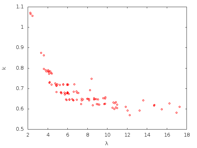
Figure 25: The Weibull parameters given simulation inputs with independent Normal distributions.

References

- Box and Tiao [1992] George E. P. Box and George C. Tiao. Bayesian Inference in Statistical Analysis (Wiley Classics Library). Wiley-Interscience, 1992.
- Cameron and Trivedi [1998] A Colin Cameron and Parvin K Trivedi. Regression Analysis of Count Data. Econometric Society Monographs. Cambridge University Press, 1998.
- Dempster et al. [1977] A P Dempster, N M Laird, and D B Rubin. Maximum likelihood from incomplete data via the EM algorithm. Journal of the Royal Statistical Society, Series B, 39(1):1–38, 1977.
- Devroye [1986] Luc Devroye. Non-Uniform Random Variate Generation. Springer-Verlag, 1986.
- Efron [2007] Bradley Efron. The future of statistics. http://www-stat.stanford.edu/~brad/talks/future.pdf, 2007.
- Efron and Gong [1983] Bradley Efron and Gail Gong. A leisurely look at the Bootstrap, the Jackknife, and cross-validation. The American Statistician, 37(1):36–48, February 1983.
- Efron and Hinkley [1978] Bradley Efron and David V Hinkley. Assessing the accuracy of the maximum likelihood estimator: Observed versus expected fisher information. Biometrika, 65(3):457–482, December 1978.
- Efron and Tibshirani [1993] Bradley Efron and Robert J Tibshirani. An Introduction to the Bootstrap. Number 57 in Monographs on Statistics and Probability. Chapman and Hall, 1993.
- Epstein and Axtell [1996] Joshua M Epstein and Robert Axtell. Growing Artificial Societies: Social Science from the Bottom Up. Brookings Institution Press, 1996.
- Fisher [1934] R A Fisher. Two new properties of mathematical likelihood. Proceedings of the Royal Society of London. Series A, Containing Papers of a Mathematical and Physical Character, 144(852):285–307, March 1934.