Microscopic description of collective properties of even-even Xe isotopes

Abstract

Collective properties of the even-even ^118-144Xe isotopes have been studied within a model employing the general Bohr Hamiltonian derived from the mean-field theory based on the UNEDF0 energy functional. The calculated low energy spectra and E2 transition probabilities are in good agreement with experimental data.

Keywords: collective model, mean-field theory, ATDHFB method, general Bohr Hamiltonian, energy density functional

1 Introduction

Currently developed mean-field theories based on energy density functionals ambitiously aim to properly explain a large range of nuclear properties and in many fields they have been quite successful. In this paper I present the results of applying of the UNEDF0 functional [1] to describe low-energy collective excitations in the chain of even-even ^118-144Xe isotopes. The treatment of collective properties is based on the Adiabatic Time Dependent HFB (ATDHFB) theory, which leads to a construction of a collective Hamiltonian from a microscopic, mean-field, input. More details of the applied methods can be found in [2, 3]. An alternative approach to collective phenomena within a microscopic theory with phenomenological interactions employs the Generator Coordinate Method (GCM), see e.g. [4, 5, 6]. One should also mention an attempt to describe collective phenomena, in the RPA context however, starting form realistic interactions and using the Unitary Correlation Operator method (UCOM) [7, 8].

For many years Xe nuclei have been subject of extensive experimental and theoretical studies. Many of them were focused on a phenomenon of the double $\beta$ decay (confirmed experimentally in the case of ¹³⁶Xe) but there is also a rich literature concerning the collective properties related to changes of nuclear deformation. The long chain of Xe isotopes offers a good opportunity to study the evolution of these properties as the number of neutrons increases as well as the role of nonaxiality. Let me mention only a few works which studied one or more of the even-even Xe isotopes: papers employing geometrical concepts and the Bohr Hamiltonian [9, 10, 2, 11, 12], papers based on the interacting boson model [13, 14, 15, 16], papers using truncated shell model space [17, 18, 19].

Section 2 presents some basic facts on the general Bohr Hamiltonian, on methods which allow for its derivation from the mean-field theory and on the UNEDF0 density energy functional. In section 3 I show the results of calculations concerning several low-spin energy levels, some E2 transitions in the ^118-144Xe nuclei as well as the comparison with experimental data.

2 Theory

2.1 Quadrupole variables, the Bohr Hamiltonian

A consistent description of nuclear vibrational and rotational excitations as well as of possible couplings between them requires the use of quadrupole collective variables i.e. of the second rank with respect to the SO(3) rotation group. Such variables can be chosen in various ways, e.g. as parameters describing the shape of a nucleus [20, 21] or the shape of a phenomenological one-particle potential [22, 9, 10]. Within a self-consistent mean field theory such quadrupole variables $\alpha_{\mu}$ (in the laboratory frame) are chosen so as to be proportional to the components of the quadrupole mass tensor

$$\alpha_{2\mu}\sim\langle\Phi|\sum_{i=1}^{A}r_{i}^{2}Y_{2\mu}(\theta_{i},\phi_{i})|\Phi\rangle$$ (1)

where $\Phi$ is a microscopic nuclear wave function which can be obtained by using effective interactions of the Skyrme [2] or the Gogny type [23, 24] or in the relativistic framework (RMF) [25, 26]. The quadrupole variables can be equivalently expressed in the intrinsic frame (also called principal axes frame) by two deformation variables $\beta$, $\gamma$ and three Euler angles ($\Omega$) describing the relative orientation of the laboratory and intrinsic frame. The $\beta$, $\gamma$ variables are given by mean values of the operators $Q_{0}=\sum^{A}_{i=1}(3z^{2}_{i}-r_{i}^{2})$ and $Q_{2}=\sum^{A}_{i=1}\sqrt{3}(x^{2}_{i}-y^{2}_{i})$ as follows

$$\beta\cos\gamma=cq_{0},\quad\quad q_{0}=\langle\Phi|Q_{0}|\Phi\rangle$$ (2)

$$\beta\sin\gamma=cq_{2},\quad\quad q_{2}=\langle\Phi|Q_{2}|\Phi\rangle$$ (3)

with a conventional factor $c=\sqrt{\pi/5}/A\overline{r^{2}}$ where $\overline{r^{2}}=3/5r^{2}_{0}A^{2/3}$, $r_{0}=1.2$ fm.

One should keep in mind that in some theoretical approaches, e.g. in the geometrical collective (Frankfurt) model [27], the deformation variables $\beta$, $\gamma$ do not have a direct relation to a nuclear shape or mass distribution. Within a framework of the interacting boson model [28] the $\beta$, $\gamma$ variables introduced by means of the so called coherent states are related rather with properties of valence nucleons and not of a spatial distribution of a nuclear density.

The general properties of the quadrupole collective space as well as of functions and operators depending on the quadrupole variables can be found e.g. in [3]. The most important, from the point of view of physical applications, is a Hamiltonian which we call the General Bohr Hamiltonian (GBH) and which can be expressed in the intrinsic frame as

$$H_{\rm Bohr}=T_{\rm vib}+T_{\rm rot}+{V}$$ (4)

$$T_{\rm vib} =-{1\over{2\sqrt{wr}}}\left\{{1\over\beta^{4}}\bigg{[}\partial_{\beta}\bigg{(}\beta^{4}\sqrt{r\over w}{B_{\gamma\gamma}}\bigg{)}\partial_{\beta}-\partial_{\beta}\bigg{(}\beta^{3}\sqrt{r\over w}{B_{\beta\gamma}}\bigg{)}\partial_{\gamma}\bigg{]}+\right.$$ (5)

$$\left.+{1\over\beta\sin\!3\gamma}\bigg{[}-\partial_{\gamma}\bigg{(}\sqrt{r\over w}\sin\!3\gamma{B_{\beta\gamma}}\bigg{)}\partial_{\beta}+{1\over\beta}\partial_{\gamma}\bigg{(}\sqrt{r\over w}\sin\!3\gamma{B_{\beta\beta}}\bigg{)}\partial_{\gamma}\bigg{]}\right\}$$

$$T_{\rm rot} ={1\over 2}\sum_{k=1}^{3}I^{2}_{k}(\Omega)/J_{k};\ \ \ \ J_{k}=4{B_{k}(\beta,\gamma)}\beta^{2}\sin^{2}(\gamma-2\pi k/3)$$ (6)

$$\ \mbox{where}\quad\quad w=B_{\beta\beta}B_{\gamma\gamma}-B^{2}_{\beta\gamma};\ \ r=B_{x}B_{y}B_{z}$$ (7)

The operators $I_{k}(\Omega),k=1,2,3$ are components of the angular momentum in the intrinsic frame. The Hamiltonian (4) contains seven functions that depend on deformation variables: the potential energy $V$ and six functions $B_{\beta\beta},B_{\beta\gamma},B_{\gamma\gamma},B_{k}$, called mass parameters or inertial functions.

One possible way to determine these seven functions consists in assuming for them a ’reasonable’ form with some free parameters which are determined through comparison of calculated and experimental collective properties. I use another approach which is based on the ATDHFB (Adiabatic Time Dependent HFB) theory and which aims at calculating these functions starting from a microscopic theory. In this approach one does not introduce any additional free parameters and the prediction of collective properties is based solely on the knowledge of effective nucleon-nucleon interactions.

2.2 The ATDHFB mass parameters

In the following discussion it is assumed that the time evolution of a system is determined through a time dependence of several collective variables $q_{j}$ (not necessarily the quadrupole ones from eqs. (2-3)). The ATDHFB theory, based on an assumption of low collective velocities, gives an expression $\frac{1}{2}\textstyle\sum_{k,j}B_{kj}\dot{q}_{k}\dot{q}_{j}$ which is bilinear in velocities and which defines a metric tensor in the collective space. In the next step this expression is used to calculate the Laplace-Beltrami operator which is taken (up to the $\hbar^{2}$ factor) as a kinetic energy part of a collective Hamiltonian. Functions $B_{kj}$ (mass parameters) depend on collective variables. More details on the ATDHFB theory and mass parameters can be found in e.g. [3, 29] and papers cited therein. Below I briefly sketch some steps and give some formulas which are needed to calculate the general Bohr Hamiltonian starting from the UNEDF0 energy functional.

The so called cranking approximation ignores the Thouless-Valatin terms so that the mass parameters can be conveniently expressed through derivatives of a generalized density matrix $R(\boldsymbol{q})$ corresponding to the HFB state $\Phi(\boldsymbol{q})$. The derivative $\displaystyle\partial_{q_{k}}R$ in the quasi-particle basis (in the doubled space) has the form

$$\left(\frac{\partial}{\partial q_{k}}R\right)_{\rm quasipart}=F_{k}=\left(\begin{array}[]{cc}0&f_{k}\\ \tilde{f}_{k}&0\end{array}\right),\ \ \ \tilde{f}_{k}=-f^{*}_{k}$$ (8)

and the mass parameters read

$$B_{kj}=\frac{\hbar^{2}}{2}\sum_{\mu\nu}\frac{f_{j,\mu\nu}f^{*}_{k,\mu\nu}+f^{*}_{j,\mu\nu}f_{k,\mu\nu}}{E_{\mu}+E_{\nu}}$$ (9)

where $E_{\mu,\nu}$ are quasi-particle energies. If the matrix $\displaystyle\partial_{q_{k}}R$ is known in a fixed single-particle basis the matrix $F_{k}$ can be calculated as

$$F_{k}={\cal B}\left(\partial_{q_{k}}R\right)_{\rm fixed,doubled}{\cal B}^{+}$$ (10)

where ${\cal B}$ is the Bogolyubov matrix for $R$

$${\cal B}=\left(\begin{array}[]{cc}U^{+}&V^{+}\\ V^{T}&U^{T}\end{array}\right).$$ (11)

Sometimes the following alternative expression for $f_{k}$ is useful

$$f_{k,\mu\nu}=\bra{\Phi}\alpha_{\nu}\alpha_{\mu}\ket{\partial_{q_{k}}\Phi}$$ (12)

where $\alpha_{\mu,\nu}$ are quasi-particle annihilation operators.

In the case of quadrupole variables one obtains the deformation-dependent HFB state by constrained HFB calculations

$$\delta\langle\Phi|H_{\rm micr}|\Phi\rangle=0\ \ \ \mbox{with}\ \ \ \langle\Phi|Q_{j}|\Phi\rangle=q_{j},\ j=0,2$$ (13)

Then, it is easier first to discuss the vibrational mass parameters $B_{q_{i}q_{k}},k=0,2$ from which $B_{\beta\beta},B_{\beta\gamma},B_{\gamma\gamma}$ in the formulas (5-7) can be calculated by a simple change of variables. The required derivatives $\partial_{q_{k}}R$ should be calculated by numerical differentiation (see [30, 2, 29]) but most often one resorts to another (so called perturbative) approximation which relates the derivatives of the generalized density matrix to derivatives of the induced one-body Hamiltonian [3]. The constraints (eq 13) lead to the extra term $-\lambda_{j}Q_{j}$ in the induced one-body Hamiltonian and one can easily calculate a derivative with respect to $\lambda_{j}$:

$$(f_{\lambda_{j}})_{\mu\nu}=\frac{1}{E_{\mu}+E_{\nu}}(w_{j})_{\mu\nu},\ \$$ (14)

where

$$w_{j}=U^{+}(Q_{j})_{\rm fixed}V^{*}-(U^{+}(Q_{j})_{\rm fixed}V^{*})^{T}$$ (15)

Then, the derivatives $\partial_{q_{k}}R$ are calculated using the relation

$$\frac{\partial}{\partial{q_{k}}}R=\sum_{j}\frac{\partial\lambda_{j}}{\partial{q_{k}}}\frac{\partial}{\partial{\lambda_{j}}}R$$ (16)

and finally the derivatives ${\partial\lambda_{j}}/{\partial{q_{k}}}$ are obtained by inverting the matrix ${\partial q_{k}}/{\partial{\lambda_{j}}}$, which can also be expressed through $w_{j}$, eq (15)

$$\frac{\partial q_{k}}{\partial{\lambda_{j}}}={\rm Re}\sum_{\mu\nu}\frac{(w_{k}^{*})_{\mu\nu}(w_{j})_{\mu\nu}}{E_{\mu}+E_{\nu}}.$$ (17)

The moments of inertia are given by the Inglis-Belyaev formula

$$J_{k}=\sum_{\mu,\nu}\frac{|[U^{+}(j_{k})_{\rm fixed}V^{*}-(U^{+}(j_{k})_{\rm fixed}V^{*})^{T}]_{\mu\nu}|^{2}}{E_{\mu}+E_{\nu}}$$ (18)

where $(j_{k})_{\rm fixed}$ is a matrix of the microscopic total angular momentum.

In the case of the BCS approximation when the canonical basis is used formulas (15, 18) can be transformed to a simpler and better known form but in the general HFB approach (15, 18) are more useful.

2.3 The UNEDF0 Energy functional

To construct the mean-field configurations I used the UNEDF0 energy density functional, which is one of the results of a large scale project UNEDF [31]. The functional is described in detail in [1] and here I will elaborate only on some of its distinctive features. In the particle-hole channel UNEDF0 is a ’standard’ Skyrme-type functional [32] with the spin-orbit term treated as in the SkI parametrization [33]. The pairing interaction is modelled as a sum of the standard (volume) plus density-dependent surface peaked $\delta$ interaction

$$\frac{{V^{q}_{0}}}{2}\left[1+\bigg{(}1-\frac{\rho(\boldsymbol{r})}{\rho_{0}}\bigg{)}\right]\delta(\boldsymbol{r}_{1}-\boldsymbol{r}_{2}),\ \ q={\rm n},{\rm p};\ \ \rho_{0}=0.16~{}{\rm fm}^{-3}$$ (19)

and the Lipkin-Nogami method is used to avoid the pairing ’collapse’ for magic nuclei and their neigbours. The pairing strengths for protons and neutrons, $V^{\rm n,p}_{0}$ are fitted simultaneously with other parameters determining the functional. A truncation of the quasi-particle space, required due to a zero-range of the pairing interaction is fixed by the condition for quasi-particle energies $E_{\mu}<60~{}{\rm MeV}$. Because it is well known that the ATDHFB mass parameters are quite sensitive to a diffuseness of the occupation number distribution I shall now present more details on the treatment of the pairing part of UNEDF0.

The binding energies of the considered Xe isotopes are reproduced quite well by the UNEDF0 functional. The RMSD (root mean square deviation) for 16 nuclei is equal to 0.454 MeV with the largest error $B_{\rm th}-B_{\rm exp}=-0.71$ MeV for the ¹³⁴Xe isotope. The chain of isotopes contains ¹³⁶Xe with a magic number $N=82$ of neutrons but it appears that due to the Lipkin-Nogami (LN) prescription the changes of the pairing properties along the chain are quite smooth. This can be seen in figure 1 where I plot the neutron and proton pairing energy vs the mass number. In addition I show a plot of the quantity $\Delta_{\rm av}+\lambda_{2,LN}$, where $\Delta_{\rm av}=\sum u_{\mu}v_{\mu}\Delta_{\mu}/\sum u_{\mu}v_{\mu}$ and $\lambda_{2,LN}$ is a coefficient determined in the LN method. This quantity can be treated as an estimation of the pairing gap within the LN method, for more details see [34].

Figure 1: Plot of the pairing energy (upper panel) and of the effective pairing gap $\Delta_{\rm av}+\lambda_{2,LN}$ calculated for protons (◆)and neutrons (○) at the deformation corresponding to a minimum of the potential energy.

In conclusion I want to mention two newer functionals UNEDF1 [35] and UNEDF2 [35, 36] which were constructed by extending the empirical dataset used in the fitting procedure. In the case of the UNEDF1 functional new data on a few fission isomers was added while for the UNEDF2 several single-particle level splittings were additionally considered. However, the RMSD for binding energies is significantly lower (around 1.4 MeV) for UNEDF0 than for UNEDF1 and UNEDF2 (around 1.9 MeV) hence the UNEDF0 functional seems to be a good choice for a pilot study of collective properties in the region of medium-heavy nuclei. A further detailed study on the consequences of UNEDF1 and UNEDF2 for collective nuclear properties is currently in progress.

3 Results of calculations, comparison with experiment

The values of inertial functions and potential energy which enter the General Bohr Hamiltonian were calculated at 144 points forming a regular grid in the sextant $(0\leq\beta\leq 0.65)\times(0\leq\gamma\leq 60^{\circ})$ in the deformation plane. The distance between the points is 0.05 and $6^{\circ}$ in the $\beta$ and $\gamma$ directions, respectively. The mean-field wave functions were obtained using the code HFODD ver. 2.49t, see [37] and references therein.

3.1 Potential energy surfaces

As can be seen in figure 2 there are three nuclei ^134-138Xe with a spherical minimum of the potential energy. Others exhibit deformed minima with $\beta_{\rm min}$ in the range $0.1-0.25$, mostly on the prolate axis except for ¹¹⁸Xe and ¹²⁸Xe which have slightly nonaxial minima with $\gamma_{\rm min}=8^{\circ}$ and $12^{\circ}$, respectively. The depths of the minima (relative to a spherical shape) are less than $2$ MeV. In figures 3 and 4 I show full plots of the potential energy on the deformation space for a representative sample of four isotopes. One can notice a rather weak dependence of the potential energy on the $\gamma$ variable ($\gamma$ softness), especially for lighter isotopes.

(a)

(b)

Figure 2: a) Value of the deformation $\beta_{\rm min}$ (left panel) and $\gamma_{\rm min}$ (right panel) at the minimum of the potential energy. (b) Depth (relative to a value at a spherical shape) of minima of the potential energy for the ^114-144Xe nuclei.

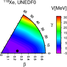
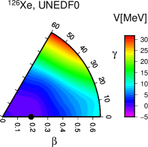
Figure 3: Plot of the potential energy (relative to a spherical shape value) for the ¹¹⁸Xe and ¹²⁶Xe isotopes.

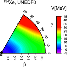
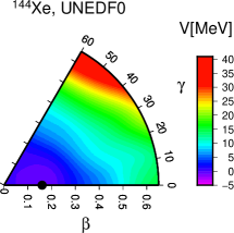
Figure 4: Plot of the potential energy (relative to a spherical shape value) for the ¹³⁴Xe and ¹⁴⁴Xe isotopes.

3.2 Collective energy levels

Having calculated the potential energy and mass parameters I performed a numerical diagonalization of the resulted Bohr Hamiltonian using the method described in [10, 2]. The obtained eigenvalues can be directly compared with excited energy levels of positive parity and the corresponding collective wave functions can be then used to calculate matrix elements of various operators, in particular of the operators of electromagnetic E2 transitions.

I should add that all mass parameters (vibrational and rotational) were multiplied before the diagonalization of the Bohr Hamiltonian by a constant factor $1.3$. The commonly quoted reasons for introducing such a factor refer to a simulation of the effects of including the Thouless-Valatin terms in the ATDHFB method or/and the effects of the so called pairing vibrations, see e.g. [23, 2, 3, 38, 39]. Some rather crude estimations of these effects give the value of the factor in the range $1.2-1.5$. However, due to a lack of sufficiently quantitative calculations this factor must be treated as an additional parameter of the theory. Before presenting the results for the whole chain of Xe isotopes I will show consequences of introducing the scaling factor for energy spectra and B(E2) probabilities in the case of ¹²⁶Xe. Figure 5 contains plots of bands built on $0_{1}$, $2_{2}$ and $0_{2}$ levels. There are two sets of theoretical results: obtained with the scaling factor ($sc=1.3$) and without the scaling ($sc=1$). One can see that the scaling produces a ’shrinking’ of the spectra leaving a general picture similar in both cases. In addition, one can see that the scaling leads to a better agreement with experimental data (showed in figure 5 as well). A sample of $B(E2)$ results (theoretical with and without scaling and experimental) is shown in figure 6. The sample contains cases with both good and worse agreement between theory and experiment. It can be seen that the effect of the scaling the mass parameters is much smaller on the B(E2) probabilities than on the values of level energies.

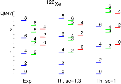
Figure 5: Energy levels in ¹²⁶Xe. Comparison of theoretical results obtained using the scaling of mass parameters ($sc=1.3$), without such scaling ($sc=1$) and experimental data.

Figure 6: Selected E2 transitions in the ¹²⁶Xe nucleus. Theoretical results with the scaling factor ($sc=1.3$), without one ($sc=1$) and experimental data [16] are shown with (□),(△) and (●), respectively

Then I compare theoretical energies of several low lying low spin levels ($2_{1},4_{1},2_{2},0_{2},0_{3}$) with experimental data [40] for the considered chain of Xe isotopes. These levels were chosen because of their role in analysing the band structure of nuclear spectra.

One can conclude from plots in figures 7-11 that in general the theoretical results are in good agreement with experimental data, especially for the lighter part of the isotope chain (up to $A=130$). One should also keep in mind that I do not fit any parameters to collective properties. Some significant discrepancies in the vicinity of $N=82$ number of neutrons are not unexpected because the ATDHFB theory tends to perform better for more collective nuclei, i.e. with a larger number of valence nucleons (let us recall that there are only four valence protons in Xe isotopes). This effect is connected with an assumption of adiabatic motion of all nucleons in the varying mean-field. This assumption is strongly affected by a presence of closed shells.

Figure 7: Experimental (■) [40] and theoretical (□) energy of the $2^{+}_{1}$ level in the ^114-144Xe nuclei.

Figure 8: Same as in figure 7, but for the $4^{+}_{1}$ level.

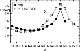
Figure 9: Same as in figure 7, but for the $2^{+}_{2}$ level.

Figure 10: Same as in figure 7, but for the $0^{+}_{2}$ level.

Figure 11: Same as in figure 7, but for the $0^{+}_{3}$ level.

3.3 E2 transitions

A detailed analysis of experimental data on electromagnetic transitions can provide important information about excited levels, see e.g. [41]. In the case of quadrupole excitations the most important are E2 transitions which are described by the collective operator

$$Q^{\rm(charge)}_{2\mu}(\beta,\gamma)=\langle\Phi(\beta,\gamma)|e\textstyle\sum_{i=1}^{Z}r_{i}^{2}Y_{2\mu}(\theta_{i},\phi_{i})|\Phi(\beta,\gamma)\rangle$$ (20)

I present the results of calculations of the B(E2) reduced transition probabilities for transitions $2_{1}\rightarrow 0_{1}$ and $4_{1}\rightarrow 2_{1}$ as well as their comparison with evaluated experimental data from [40] in figures 12 and 13. Again one can see that theoretical calculations reproduce the general behaviour of B(E2) quite well even as no free parameters (e.g. effective charges) were used.

Figure 12: Experimental (●) [40] and theoretical (□) B(E2) probability (in W.u.) for the transition $2^{+}_{1}\rightarrow 0^{+}_{1}$ level in the ^114-144Xe nuclei.

Figure 13: Experimental (●) [40] and theoretical (□) B(E2) probability (in W.u.) for the transition $4^{+}_{1}\rightarrow 2^{+}_{1}$ level in the ^114-144Xe nuclei.

In the case of some Xe isotopes there are much more extensive experimental data on E2 transitions, see e.g. for ¹²⁶Xe [16] and for ¹²⁸Xe [42, 43] but I postpone a discussion of them to a subsequent publication.

4 Conclusions

The paper presents the results of the first attempt to apply the UNEDF0 energy functional to the theory of a nuclear collective motion. A correct description of the properties of the long chain of Xe isotopes considered is a demanding challenge to the theory, in particular to a framework with no free parameters that could be fitted to experimental data on collective levels. It can be argued that the results shown in section 3 are quite satisfactory and reproduce well the general tendencies seen in the energy spectra as well as E2 transitions in the Xe isotopes, with some exceptions around the semi-magic ¹³⁶Xe isotope. This contribution contains only a part of the obtained theoretical results, a more detailed analysis of the ^120-128Xe nuclei is in preparation.

References

References

- [1] Kortelainen M, Lesinski T, More J, Nazarewicz W, Sarich J, Schunck N, Stoitsov M V and Wild S 2010 Phys. Rev. C 82 024313
- [2] Próchniak L, Quentin P, Samsoen D and Libert J 2004 Nucl. Phys. A 730 59
- [3] Próchniak L and Rohoziński S G 2009 J. Phys. G (London) 36 123101
- [4] Rodriguez T R and Egido J L 2010 Phys. Rev. C 81 064323
- [5] Yao J M, Bender M and Heenen P H 2013 Phys. Rev. C 87 034322
- [6] Bender M and Heenen P H 2008 Phys. Rev. C 78 024309
- [7] Papakonstantinou P, Hergert H, Ponomarev V Y and Roth R 2014 Phys. Rev. C 89 034306
- [8] Papakonstantinou P, Roth R and Paar N 2007 Phys. Rev. C 75 014310
- [9] Rohoziński S G, Dobaczewski J, Nerlo-Pomorska B, Pomorski K and Srebrny J 1977 Nucl. Phys. A 292 66
- [10] Próchniak L, Zajac K, Pomorski K, Rohoziński S G and Srebrny J 1999 Nucl. Phys. A 648 181
- [11] Hinohara N, Li Z P, Nakatsukasa T, Niksic T and Vretenar D 2012 Phys. Rev. C 85 024323
- [12] Bonatsos D, Georgoudis P E, Minkov N, Petrellis D and Quesne C 2013 Phys. Rev. C 88 034316
- [13] von Brentano P, Gelberg A, Harissopulos S and Casten R F 1988 Phys. Rev. C 38 2386
- [14] Krips W, Frank W, Lieberz W and von Brentano P 1991 Nucl. Phys. A 529 485
- [15] Sorgunlu B and Isacker P V 2008 Nucl. Phys. A 808 27
- [16] Coquard L, Rainovski G, Pietralla N, Ahn T, Bettermann L, Carpenter M P, Janssens R V F, Leske J, Lister C J, Moller O, Moller T, Rother W, Werner V and Zhu S 2011 Phys. Rev. C 83 044318
- [17] Pan X W, Ping J L, Feng D H, Chen J Q, Wu C L and Guidry M W 1996 Phys. Rev. C 53 715
- [18] Meng X, Wang F, Luo Y, Pan F and Draayer J P 2008 Phys. Rev. C 77 047304
- [19] Higashiyama K and Yoshinaga N 2011 Phys. Rev. C 83 034321
- [20] Bohr A 1952 Mat. Fys. Medd. Dan. Vid. Selsk. 26 no. 14, 1
- [21] Bohr A and Mottelson B R 1969 Nuclear Structure, vol. I (Benjamin Inc)
- [22] Kaniowska T, Sobiczewski A, Pomorski K and Rohoziński S G 1976 Nucl. Phys. A 274 151
- [23] Libert J, Girod M and Delaroche J P 1999 Phys. Rev. C 60 054301
- [24] Delaroche J P, Girod M, Libert J, Goutte H, Hilaire S, Peru S, Pillet N and Bertsch G F 2010 Phys. Rev. C 81 014303
- [25] Próchniak L and Ring P 2004 Int. J. Mod. Phys. E 13 217
- [26] Niksic T, Li Z P, Vretenar D, Próchniak L, Meng J and Ring P 2009 Phys. Rev. C 79 034303
- [27] Eisenberg J and Greiner W 1985 Nuclear Theory Vol. 1: Nuclear Models 3rd ed (North Holland Physics Publ.)
- [28] Iachello F and Arima A 1975 The Interacting Boson Model (Cambridge University Press)
- [29] Baran A, Sheikh J A, Dobaczewski J, Nazarewicz W and Staszczak A 2011 Phys. Rev. C 84 054321
- [30] Yuldashbaeva E K, Libert J, Quentin P and Girod M 1999 Phys. Lett. B 461 1
- [31] Bogner S, Bulgac A, Carlson J, Engel J, Fann G, Furnstahl R J, Gandolfi S, Hagen G, Horoi M, Johnson C, Kortelainen M, Lusk E, Maris P, Nam H, Navratil P, Nazarewicz W, Ng E, Nobre G P A, Ormand E, Papenbrock T, Pei J, Pieper S C, Quaglioni S, Roche K J, Sarich J, Schunck N, Sosonkina M, Terasaki J, Thompson I, Vary J P and Wild S M 2013 Comp. Phys. Comm. 184 2235–2250
- [32] Bender M, Heenen P H and Reinhard P G 2003 Rev. Mod. Phys. 75 121
- [33] Reinhard P G and Flocard H 1995 Nucl. Phys. A 584 467
- [34] Bender M, Rutz K, Reinhard P G and Maruhn J A 2000 Eur. Phys. J. A 8 59
- [35] Kortelainen M, McDonnell J, Nazarewicz W, Reinhard P G, Sarich J, Schunck N, Stoitsov M V and Wild S M 2012 Phys. Rev. C 85 024304
- [36] Kortelainen M, McDonnell J, Nazarewicz W, Olsen E, Reinhard P G, Sarich J, Schunck N, Wild S M, Davesne D, Erler J and Pastore A 2014 Phys. Rev. C 89 054314
- [37] Schunck N, Dobaczewski J, McDonnell J, Satuła W, Sheikh J A, Staszczak A, Stoitsov M and Toivanen P 2012 Comp. Phys. Comm. 183 166–192
- [38] Próchniak L 2007 Int. J. Mod. Phys. E 16 352
- [39] Li Z P, Niksic T, Vretenar D and Meng J 2010 Phys. Rev. C 81 034316
- [40] Data extracted using the NNDC On-Line Data Service from the ENSDF database, file revised as of September 2014.
- [41] Wrzosek-Lipska K, Próchniak L, Zielińska M, Srebrny J, Hadyńska-Klek K, Iwanicki J, Kisieliński M, Kowalczyk M, Napiorkowski P J, Pietak D and Czosnyka T 2012 Phys. Rev. C 86 064305
- [42] Srebrny J, Czosnyka T, Karczmarczyk W, Napiorkowski P, Droste C, Wollersheim H J, Emling H, Grein H, Kulessa R, Cline D and Fahlander C 1993 Nucl. Phys. A 557 663c
- [43] Coquard L, Pietralla N, Ahn T, Rainovski G, Bettermann L, Carpenter M P, Janssens R V F, Leske J, Lister C J, Moller O, Rother W, Werner V and Zhu S 2009 Phys. Rev. C 80 061304