A comparative review of generalizations of
the Gumbel extreme value distribution
with an application to wind speed data

Abstract

The generalized extreme value distribution and its particular case, the Gumbel extreme value distribution, are widely applied for extreme value analysis. The Gumbel distribution has certain drawbacks because it is a non-heavy-tailed distribution and is characterized by constant skewness and kurtosis. The generalized extreme value distribution is frequently used in this context because it encompasses the three possible limiting distributions for a normalized maximum of infinite samples of independent and identically distributed observations. However, the generalized extreme value distribution might not be a suitable model when each observed maximum does not come from a large number of observations. Hence, other forms of generalizations of the Gumbel distribution might be preferable. Our goal is to collect in the present literature the distributions that contain the Gumbel distribution embedded in them and to identify those that have flexible skewness and kurtosis, are heavy-tailed and could be competitive with the generalized extreme value distribution. The generalizations of the Gumbel distribution are described and compared using an application to a wind speed data set and Monte Carlo simulations. We show that some distributions suffer from overparameterization and coincide with other generalized Gumbel distributions with a smaller number of parameters, i.e., are non-identifiable. Our study suggests that the generalized extreme value distribution and a mixture of two extreme value distributions should be considered in practical applications.

Key words: Generalized extreme value distribution; Gumbel distribution; Heavy-tailed distribution; Non-identifiable model; Kurtosis; Wind speed.

1 Introduction

Extreme value data usually exhibit excess kurtosis and/or heavy right tails. This is particularly common in environmental data, e.g., maximum water level (Bruxer et al., 2008), maximum wind speed (Castillo et al., 2005, Examples 6.1 and 9.14), spatial and temporal variability of turbulence (Sanford, 1997), daily maximum ozone measurement (Gilleland, 2005), and largest lichen measurements (Cooley et al., 2006). The generalized extreme value distribution (GEV) is fairly well-accepted as a standard working model. Despite such well-established theory, extreme-value distributions are not always preferred in studies of empirical data that do not contemplate the conditions to use extreme value theory results. Sometimes, the fit for finite samples is poor. To surpass these issues, other generalizations of the Gumbel distribution were proposed. For instance, Hosking (1994) proposed a four-parameter distribution to model the maximum precipitation data that has been used in many fields including environmental sciences, see Hosking & Wallis (1997), Parida (1999), Park & Jung (2002), and Sing & Deng (2003); Reed & Robson (1999, §17.3.2) recommends a particular three-parameter generalized logistic distribution as preferable to a GEV distribution for UK annual flood maximum.

The Gumbel distribution, also known as the extreme value distribution or the Gumbel extreme value distribution, is also used to model extreme values (Coles, 2001; Castillo et al., 2005; Ferrari & Pinheiro, 2012, 2015). However, its skewness and kurtosis coefficients are constant, and its right tail is light. Generalizations of the Gumbel distribution with flexible skewness and kurtosis coefficients could provide better fits for extreme value data.

We present a comprehensive comparative review of distributions that contain the Gumbel distribution as a special or limiting case. We note that certain generalizations of the Gumbel distribution proposed in the literature are not identifiable.  Some distributions suffer from overparameterization and coincide with other generalized Gumbel distributions with a smaller number of parameters. As noted by Huang (2005) “when applying a nonidentifiable model, different people may draw different conclusions from the same model of the observed data. Before one can meaningfully discuss the estimation of a model, model identifiability must be verified.” Therefore, we distinguish between the identifiable and nonidentifiable models and limit our study to the identifiable family of distributions only.

We investigate and compare the relevant properties of the selected distributions. In particular, we derive their coefficients of skewness and kurtosis, which are invariant under location-scale transformations and are primarily controlled by the extra parameters. We graphically illustrate their flexibility relative to the Gumbel distribution and highlight those that can achieve high values of skewness and kurtosis with a heavy right tail.

Danielsson et al. (2006) stated “heavy-tailed distributions are often defined in terms of higher than normal kurtosis. However, the kurtosis of a distribution may be high if either the tails of the cumulative distribution function are heavier than the normal or the center is more peaked or both.” Moment-based measures suffer from effects from an extreme tail of the distribution, which may have negligible probability. These characteristics motivated us to study the tail behavior of the distributions specifically. To mathematically classify the tail behavior of distributions, we employ regular variation theory (de Haan, 1970) and a criterion proposed by Rigby et al. (2014) based on an approximation of the logarithm of the probability density function.

Additionally, we conduct a comprehensive simulation study to evaluate the flexibility of each selected distribution in fitting data sets generated from the Gumbel distribution and its different generalizations. The simulated data sets cover a reasonable range of skewness, kurtosis and tail heaviness behaviors. We compare the different distributions through the analysis of a data set on the maximum monthly wind speed in West Palm Beach, Florida, for the years 1984-2014.

The paper is organized as follows. In Section 2, we present the Gumbel distribution and its generalizations. In Section 3, we study the right tail heaviness of the identifiable distributions. Monte Carlo simulations are presented in Section 4, and an application to a real data set is provided in Section 5. The paper ends with conclusions in Section 6. Technical details are given in the Supplement.

2 The Gumbel distribution and its generalizations

We present selected characteristics of the Gumbel distribution and distributions that contain the Gumbel distribution as a special or limiting case. For the identifiable distributions, the moments, $p$-quantile ($x_{p}$), skewness ($\gamma_{1}$) and kurtosis ($\gamma_{2}$) coefficients are summarized in the Supplement. Random draws from distributions with closed-form $p$-quantiles can be generated by replacing $p$ with a standard uniform distributed observation. For the others, generating methods are given.

Gumbel distribution (EV).

Let $X\sim{\rm EV}_{max}(\mu,\sigma)$ be a continuous random variable with a maximum extreme value distribution. The probability density function (pdf) and cumulative distribution function (cdf) are, respectively,

$$f_{{\rm EV}_{max}}(x;\mu,\sigma)=\frac{1}{\sigma}\exp\left(-\frac{x-\mu}{\sigma}\right)\exp\left\{-\exp\left(-\frac{x-\mu}{\sigma}\right)\right\},\quad x\in I\!\!R,$$ (1)

$$F_{{\rm EV}_{max}}(x;\mu,\sigma)=\exp\left(-\exp\left(-\frac{x-\mu}{\sigma}\right)\right),\quad x\in I\!\!R,$$ (2)

where $\mu\in I\!\!R$ is the location parameter and $\sigma>0$ is the scale parameter. This distribution is also known as the Gumbel or type I extreme value distribution. The distribution in (1) is one of the three possible limiting laws of the standardized maximum of independent and identically distributed random variables (Gnedenko, 1943). It is frequently invoked to model extreme events; see, e.g., Castillo et al. (2005, Table 9.16) and Coles (2001, Section 3.4.1). We refer to this distribution as the maximum extreme value distribution to distinguish it from the minimum extreme value distribution, which is also often known as the Gumbel or type I extreme value distribution in the statistical literature.

The coefficients of skewness and kurtosis of the Gumbel distribution are constant $\gamma_{1,{\rm EV}}=1.14$ and $\gamma_{2,{\rm EV}}=5.4$, respectively, i.e., parameter independent. This restriction motivates more flexible and useful generalizations of the Gumbel distribution to fit real data.

Hereafter, the maximum extreme value or Gumbel variable will be referred to as Gumbel and denoted by EV.

Generalized extreme value distribution (GEV).

The generalized extreme value distribution (GEV) was defined for the first time by Jenkinson (1955), and the three possible limiting distributions of the maximum/minimum of random variables are embedded within it. This distribution is also known as the von Mises extreme value, von Mises-Jenkinson, and Fisher-Tippet distribution. A historical review of extreme value theory, the main results, and a list of several areas of application are provided in Kotz & Nadajarah (2000).

Let $X\sim{\rm GEV}(\mu,\sigma,\alpha)$ be a generalized extreme value distributed random variable. Its pdf and cdf are, respectively,

$$f_{{\rm GEV}}(x;\mu,\sigma,\alpha)=\frac{1}{\sigma}{\rm exp}\left(-\left[1+\alpha\left(\frac{x-\mu}{\sigma}\right)\right]^{-1/\alpha}\right)\left[1+\alpha\left(\frac{x-\mu}{\sigma}\right)\right]^{-1/\alpha-1},$$

and

$$F_{{\rm GEV}}(x;\mu,\sigma,\alpha)={\rm exp}\left(-\left[1+\alpha\left(\frac{x-\mu}{\sigma}\right)\right]^{-1/\alpha}\right),\quad\{x:1+\alpha(x-\mu)/\sigma>0\},$$

where $\alpha\in I\!\!R$. The Gumbel distribution is a particular case of the GEV distribution when $\alpha\rightarrow 0$.

Plots of the pdf and the .99 quantile of GEV$(0,1,\alpha)$, and the skewness and kurtosis of GEV$(\mu,\sigma,\alpha)$ for selected values of $\alpha$ are shown in Figure 1. The GEV distribution is quite versatile, and $\alpha$ has a substantial effect on its skewness and kurtosis. The parameter $\alpha$ affects location, dispersion, skewness and kurtosis. Increasing values of $\alpha$ increases the quantiles, skewness and kurtosis coefficients, and right-tail heaviness. Skewness is defined for $\alpha<1/3$ and kurtosis for $\alpha<1/4$. Skewness and kurtosis can assume different values from those of the Gumbel distribution.

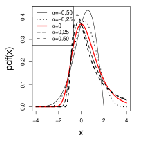
Figure 1: Density function and .999 quantile - GEV$(0,1,\alpha)$; skewness and kurtosis - GEV$(\mu,\sigma,\alpha)$

Exponentiated Gumbel distribution (EGu).

Let $X\sim{\rm EGu}(\mu,\sigma,\alpha)$ be an exponentiated Gumbel distributed random variable. Its pdf and cdf are, respectively,

$$f_{{\rm EGu}}(x;\mu,\sigma,\alpha)=\frac{\alpha}{\sigma}\exp\left(-\frac{x-\mu}{\sigma}\right)\exp\left(-\exp\left(-\frac{x-\mu}{\sigma}\right)\right)\left[1-\exp\left(-\exp\left(-\frac{x-\mu}{\sigma}\right)\right)\right]^{\alpha-1},$$

$x\in I\!\!R,$ and

$$F_{{\rm EGu}}(x;\mu,\sigma,\alpha)=1-\left[1-\exp\left(-\exp\left(-\frac{x-\mu}{\sigma}\right)\right)\right]^{\alpha},\quad x\in I\!\!R,$$

where $\alpha>0$ (Nadarajah, 2006). The Gumbel distribution is a special case of the EGu distribution when $\alpha=1$.

The pdf can be written as

$$f_{{\rm EGu}}(x;\mu,\sigma,\alpha)=$$

$$\frac{\alpha}{\sigma}\exp\left(-\frac{x-\mu}{\sigma}\right)\exp\left(-\exp\left(-\frac{x-\mu}{\sigma}\right)\right)\;_{2}F_{1}\left(1-\alpha,1;1;\exp\left(-\exp\left(-\frac{x-\mu}{\sigma}\right)\right)\right),$$

where ${}_{2}F_{1}(a,b;c;z)=\sum_{k=0}^{\infty}[(a)_{k}(b)_{k}/(c)_{k}][z^{k}/k!]$ for $|z|<1$ is the hypergeometric function, $(a)_{k}=\Gamma(a+k)/\Gamma(a)$ is the Pochhammer symbol and $\Gamma(\cdot)$ is the gamma function. Thus ${}_{2}F_{1}(a,1;1;z)=\sum_{k=0}^{\infty}(a)_{k}z^{k}/k!=(1-z)^{-a}$ for $|z|<1$. Note that $\left|\exp\left(-\exp\left(-(x-\mu)/(\sigma)\right)\right)\right|<1$. This form of the pdf is computationally highly efficient for evaluating moments of the EGu distribution if using software that contains an optimized implementation of the hypergeometric function.

The right tail is heavier for smaller values of $\alpha>0$ (Figure 2). When $\alpha$ is close to zero, minor changes in $\alpha$ lead to significant changes in the quantile values. The skewness and kurtosis can reach values close to 2 and 9, respectively, indicating that the EGu distribution is more flexible than the Gumbel distribution.

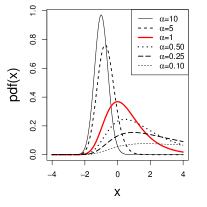
Figure 2: Density function and .99 quantile - EGu$(0,1,\alpha)$; skewness and kurtosis - EGu$(\mu,\sigma,\alpha)$

Transmuted extreme value distribution (TEV).

Shaw & Buckley (2009) defined a transformation known as the rank transmutation map, with the aim of obtaining distributions with skewness and kurtosis distinct from those of the normal distribution.

Transmutation is a composite map of a cumulative distribution function with a quantile function of another distribution defined on the same sample space. A particular case of rank transmutation map is derived by considering

$$T_{R}(u)=F_{2}(F_{1}^{-1}(u))=u+\alpha u(1-u),$$

which leads to

$$F_{2}(x)=(1+\alpha)F_{1}(x)-\alpha F_{1}^{2}(x),$$

for $|\alpha|\leq 1$, known as the quadratic rank transmutation. There are two important boundary cases. When $\alpha=-1$, $F_{2}(x)=F_{1}(x)^{2}$, i.e., $F_{2}$ is the distribution of the maximum of two independent variables with distribution $F_{1}$. Analogously, when $\alpha=1$, $F_{2}$ is the distribution of the minimum. Motivated by the various applications of the extreme value theory, particularly the Gumbel distribution, Aryal & Tsokos (2009) defined a new distribution known as the transmuted extreme value distribution (TEV) by replacing $F_{1}$ with a Gumbel cdf.

Let $X\sim{\rm TEV}(\mu,\sigma,\alpha)$ be a transmuted extreme value distributed random variable. Its pdf and cdf are, respectively,

$$f_{{\rm TEV}}(x;\mu,\sigma,\alpha)=\frac{1}{\sigma}\exp\left[-\frac{x-\mu}{\sigma}-\exp\left(-\frac{x-\mu}{\sigma}\right)\right]\left[1+\alpha-2\alpha\exp\left(-\exp\left(-\frac{x-\mu}{\sigma}\right)\right)\right],$$

$$x\in I\!\!R,$$

and

$$F_{{\rm TEV}}(x;\mu,\sigma,\alpha)=(1+\alpha)\exp\left[-\exp\left(-\frac{x-\mu}{\sigma}\right)\right]-\alpha\exp\left[-2\exp\left(-\frac{x-\mu}{\sigma}\right)\right],\quad x\in I\!\!R,$$

where $|\alpha|\leq 1$. The Gumbel distribution is a particular case of the TEV distribution when $\alpha=-1$ or $\alpha=0$. Note that to make the TEV$(\mu,\sigma,\alpha)$ family of distributions identifiable, it is sufficient to restrict $\alpha$ to the set $(-1,1]$.

The TEV distribution is more flexible relative to the Gumbel distribution but less flexible than the GEV and EGu distributions, with maximum .99 quantile (for $\mu=0$ and $\sigma=1$) and coefficients of skewness and kurtosis lower than 6, 2 and 7, respectively (Figure 3). Note that from the pdf and .99 quantile plots, the right tail gets heavier for smaller values of $-1<\alpha\leq 1$.

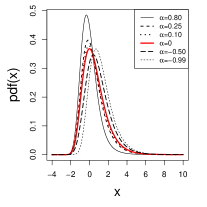
Figure 3: Density function and .99 quantile - TEV$(0,1,\alpha)$; skewness and kurtosis - TEV$(\mu,\sigma,\alpha)$

Kumaraswamy Gumbel distribution.

Cordeiro et al. (2012) defined a generalization of a cdf $G(x)$ from the Kumaraswamy distribution, which they referred to as Kum-G. The cdfs of the Kumaraswamy and Kum-G distributions are given, respectively, by

$$F_{{\rm Kum}}(x;\alpha,\beta)=1-\{1-x^{\alpha}\}^{\beta},\quad x\in(0,1),$$

and

$$F_{{\rm Kum}{\texttt{-}}{\rm G}}(x;\alpha,\beta)=1-\{1-G(x)^{\alpha}\}^{\beta},\quad x\in I\!\!R,$$

where $\alpha>0$ and $\beta>0$. If the distribution $G(x)$ is EV$(\mu,\sigma)$, the cdf is defined by

$$F_{{\rm KumGum}}(x;\mu,\sigma,\alpha,\beta)=1-\left[1-\left(\exp\left(-\exp\left(-\frac{x-\mu}{\sigma}\right)\right)\right)^{\alpha}\right]^{\beta},\quad x\in I\!\!R,$$

where $\alpha>0$ and $\beta>0$.

Note that if $X\sim{\rm KumGum}(\mu,\sigma,\alpha,\beta)$, then

$$F_{{\rm KumGum}}(x;\mu,\sigma,\alpha,\beta) = 1-[1-\exp(-\exp(-(x-\mu^{*})/\sigma))]^{\beta}$$

$$= F_{{\rm KumGum}}(x;\mu^{*},\sigma,1,\beta)=F_{{\rm EGu}}(x;\mu^{*},\sigma,\beta),$$

where $\mu^{*}=\mu+\sigma\ln\alpha$. Therefore, the Kumaraswamy Gumbel family of distributions KumGum $(\mu,\sigma,\alpha,\beta)$, where $\alpha>0$ and $\beta>0$, is nonidentifiable. It coincides with the exponentiated Gumbel family of distributions EGu$(\mu^{*},\sigma,\beta)$, where $\mu^{*}\in I\!\!R$, $\sigma>0$ and $\beta>0$. In other words, the Kumaraswamy Gumbel family of distributions has four parameters but corresponds to a family with only three parameters. This is a typical case of parameter redundancy, i.e., overparameterization (Catchpole & Morgan, 1997). Therefore, this distribution will not be contemplated hereafter.

Generalized three-parameter Gumbel distribution (GTIEV3).

Dubey (1969) built a generalization of the Gumbel distribution which is known as the generalized type I extreme value or type I generalized logistic distribution, and we denote it by GTIEV$(\mu,\sigma,\alpha,\beta)$. Its cdf is given by

$$F_{{\rm GTIEV}}(x;\mu,\sigma,\alpha,\beta)=\left(1+\frac{\sigma}{\beta}\exp\left(-\frac{x-\mu}{\sigma}\right)\right)^{-\alpha},\quad x\in I\!\!R,$$

where $\alpha>0$ and $\beta>0$. This distribution was first defined by Hald (1952). Note that

$$F_{{\rm GTIEV}}(x;\mu,\sigma,\alpha,\beta)=\left(1+\frac{1}{\alpha}\exp\left(-\frac{x-\mu^{*}}{\sigma}\right)\right)^{-\alpha},\quad x\in I\!\!R,$$

where $\mu^{*}=\mu+\sigma\ln(\sigma\alpha\beta^{-1})\in I\!\!R$. Therefore, the generalized Gumbel family GTIEV$(\mu,\sigma,\alpha,\beta)$, where $\mu\in I\!\!R$, $\sigma>0$, $\alpha>0$, and $\beta>0$, is nonidentifiable. It coincides with a family of distributions with only three parameters, say GTIEV3$(\mu,\sigma,\alpha)$, where $\mu\in I\!\!R$, $\sigma>0$ and $\alpha>0$.

Let $X\sim{\rm GTIEV}3(\mu,\sigma,\alpha)$ be a generalized three-parameter Gumbel random variable. Its pdf and cdf are defined, respectively, as

$$f_{{\rm GTIEV}3}(x;\mu,\sigma,\alpha)=\frac{1}{\sigma}\left(1+\frac{1}{\alpha}\exp\left(-\frac{x-\mu}{\sigma}\right)\right)^{-\alpha-1}\exp\left(-\frac{x-\mu}{\sigma}\right),\quad x\in I\!\!R,$$

and

$$F_{{\rm GTIEV}3}(x;\mu,\sigma,\alpha,\beta)=\left(1+\frac{1}{\alpha}\exp\left(-\frac{x-\mu}{\sigma}\right)\right)^{-\alpha},\quad x\in I\!\!R,$$

where $\alpha>0$. The Gumbel distribution is a limiting case of GTIEV3 when $\alpha\rightarrow\infty$. The three-parameter kappa distribution defined in Jeong et al. (2014, eq. 2) with positive shape parameter coincides with the GTIEV3 distribution in a different parameterization.

The GTIEV3 distribution is more flexible than the Gumbel distribution but less flexible relative to the GEV and EGu distributions (Figure 4). The .99 quantile and skewness coefficient are always lower than the corresponding Gumbel values whereas the kurtosis can be greater. The right tail of the GTIEV3 distribution can not be heavier than that of the Gumbel distribution, in contrast to its left tail. This observation suggests that the GTIEV3 distribution is not useful for modeling right-skewed data.

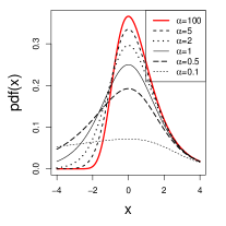
Figure 4: Density function and .99 quantile - GTIEV3$(0,1,\alpha)$; skewness and kurtosis - GTIEV3$(\mu,\sigma,\alpha)$

Three-parameter exponential-gamma distribution (EGa).

Ojo (2001) presents a generalization of the Gumbel distribution, with three parameters $\mu$, $\sigma$, and $\alpha$. We refer to it as the three-parameter exponential-gamma distribution and denote it by EGa$(\mu,\sigma,\alpha)$.

Let $X\sim\rm{EGa}(\mu,\sigma,\alpha)$ be an exponential-gamma distributed random variable. Its pdf and cdf are, respectively,

$$f_{{\rm EGa}}(x;\mu,\sigma,\alpha)=\frac{1}{\Gamma(\alpha)}\frac{1}{\sigma}\exp\left(-\exp\left(-\frac{x-\mu}{\sigma}\right)\right)\exp\left(-\alpha\frac{x-\mu}{\sigma}\right),\quad x\in I\!\!R,$$

and

$$F_{{\rm EGa}}(\mu,\sigma,\alpha)=\frac{1}{\Gamma(\alpha)}\Gamma\left(\alpha,\exp\left(-\frac{x-\mu}{\sigma}\right)\right),\quad x\in I\!\!R,$$

where $\alpha>0$, and $\Gamma(s,x)=\int_{x}^{\infty}t^{s-1}\exp(-t)dt$ is the incomplete gamma function. The Gumbel distribution is a particular case of EGa when $\alpha=1$. To generate $X\sim{\rm EGa}(\mu,\sigma,\alpha)$, we write $X=\mu-\sigma\ln(Y)$, where $Y\sim{\rm gamma}(\alpha,1)$.

Similarly to the EGu distribution, the right tail gets heavier for smaller values of $\alpha>0$ (Figure 5). For $\alpha$ close to zero, the .99 quantile can be greater than that of the Gumbel, TEV and GTIEV3 distributions. The .99 quantile plots indicate that when $\alpha$ is close to zero, small changes in $\alpha$ lead to significant changes in the quantile values; similarly to the EGu distribution, the skewness and kurtosis can reach values close to 2 and 9, respectively, indicating more flexibility than the Gumbel distribution.

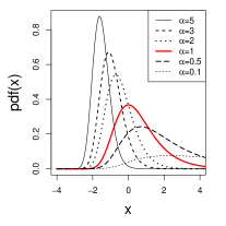
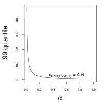
Figure 5: Density function and .99 quantile - EGa$(0,1,\alpha)$; skewness and kurtosis - EGa$(\mu,\sigma,\alpha)$

Generalized Gumbel distribution (GGu)

Cooray (2010) derived a distribution which is referred to as the generalized Gumbel distribution (GGu).

Let $X\sim{\rm GGu}(\mu,\sigma,\alpha)$ be a generalized Gumbel distributed random variable. Its pdf and cdf are, respectively,

$$f_{GGu}(x;\mu,\sigma,\alpha) = \frac{\alpha}{\sigma}\exp\left(-\frac{x-\mu}{\sigma}\right)\exp\left(\exp\left(-\frac{x-\mu}{\sigma}\right)\right)\left(\exp\left(\exp\left(-\frac{x-\mu}{\sigma}\right)\right)-1\right)^{-\alpha-1}$$

$$\left(1+\left(\exp\left(\exp\left(-\frac{x-\mu}{\sigma}\right)\right)-1\right)^{-\alpha}\right)^{-2},\;\;x\in I\!\!R,$$

and

$$F_{GGu}(x;\mu,\sigma,\alpha)=1-\left(1+\left(\exp\left(\exp\left(-\frac{x-\mu}{\sigma}\right)\right)-1\right)^{-\alpha}\right)^{-1},\;\;x\in I\!\!R,$$

where $\mu\in I\!\!R$, $\sigma>0$ and $\alpha>$. When $\alpha=1$, the GGu distribution reduces to a Gumbel distribution. Figure 6 shows the plots of the pdf for selected parameters, and the .99 quantile, skewness and kurtosis of GGu$(0,1,\alpha)$. Similarly to the EGu and EGa distributions, for $\alpha$ close to zero, the .99 quantile can be greater than that of the Gumbel, TEV and GTIEV3 distributions. The .99 quantile plot indicate that when $\alpha$ is close to zero, small changes in $\alpha$ lead to significant changes in the quantile values; the skewness and kurtosis can reach values greater than those of the Gumbel distribution.

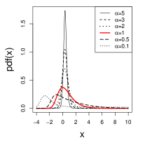
Figure 6: Density function, .99 quantile, skewness and kurtosis - GGu$(0,1,\alpha)$

Exponential-gamma distribution.

As a generalization of the Gumbel distribution, Adeyemi & Ojo (2003) proposed the asymptotic distribution of the $r$-th maximum extremes obtained by Gumbel (1935), whose pdf is

$$f(x;\mu,\sigma,\alpha)=\frac{r^{r}}{\Gamma(r)}\exp(-r\exp(-x))\exp(-rx),\quad x\in I\!\!R,$$

for $r>0$, the shape parameter. When $r=1$, this distribution reduces to a Gumbel distribution. Its generalized form is known as the exponential-gamma distribution ExpGama$(\mu,\sigma,\alpha,\beta)$ (Balakrishnan & Leung, 1988, p. 34) and is defined by the pdf and cdf given by, respectively,

$$f_{{\rm ExpGama}}(x;\mu,\sigma,\alpha,\beta)=\frac{\alpha^{\beta}}{\sigma\Gamma(\beta)}\exp\left(-\alpha\exp\left(-\frac{x-\mu}{\sigma}\right)\right)\exp\left(-\beta\frac{x-\mu}{\sigma}\right),\quad x\in I\!\!R,$$

and

$$F_{{\rm ExpGama}}(x;\mu,\sigma,\alpha,\beta)=\frac{1}{\Gamma(\beta)}\Gamma\left(\beta,\alpha\exp\left(-\frac{x-\mu}{\sigma}\right)\right),\quad x\in I\!\!R,$$

where $\alpha\in I\!\!R$ and $\beta>0$. When $\alpha=\beta=1$, the exponential-gamma distribution reduces to a Gumbel distribution, and it reduces to the EGa distribution when $\alpha=1$. Note that, if $X\sim{\rm ExpGama}(\mu,\sigma,\alpha,\beta)$ then

$$F_{{\rm ExpGama}}(x;\mu,\sigma,\alpha,\beta)=\frac{\Gamma(\beta,\exp\left(-\frac{x-\mu^{*}}{\sigma}\right))}{\Gamma(\beta)}=F_{{\rm ExpGama}}(x;\mu^{*},\sigma,1,\beta)=F_{{\rm EGa}}(x;\mu^{*},\sigma,\beta),$$

where $\mu^{*}=\mu+\sigma\ln\alpha\in I\!\!R$. Hence, the exponential-gamma family of distributions ExpGama$(\mu,\sigma,\alpha,\beta)$, where $\mu\in I\!\!R$, $\sigma>0$, $\alpha>0$ and $\beta>0$, is nonidentifiable. It coincides with the three-parameter exponential-gamma family of distributions EGa$(\mu,\sigma,\beta)$, where $\mu\in I\!\!R$, $\sigma>0$ and $\beta>0$. Therefore, this distribution will not be contemplated hereafter.

Type IV generalized logistic distribution (GLIV).

Prentice (1975) proposed the type IV generalized distribution (GLIV). Let $X\sim{\rm GLIV}(\mu,\sigma,\alpha,\beta)$ be a type IV generalized distributed random variable. Its pdf and cdf are, respectively,

$$f_{{\rm GLIV}}(x;\mu,\sigma,\alpha,\beta)=\left(\frac{\alpha}{\beta}\right)^{\alpha}\frac{1}{\sigma B(\alpha,\beta)}\frac{[\exp(-(x-\mu)/\sigma)]^{\alpha}}{[1+(\alpha/\beta)\exp(-(x-\mu)/\sigma)]^{\alpha+\beta}},\;\;x\in I\!\!R,$$

and

$$F_{{\rm GLIV}}(x;\mu,\sigma,\alpha)=$$

$$\frac{1}{\beta B(\alpha,\beta)}\left(\frac{\beta}{\alpha}\exp\left(\frac{x-\mu}{\sigma}\right)\right)^{\beta}\!_{2}F_{1}\left(\beta,\alpha+\beta;1+\beta;-\frac{\beta}{\alpha}\exp\left(\frac{x-\mu}{\sigma}\right)\right),\;\;x\in I\!\!R,$$

where $\alpha>0$, $\beta>0$ and ${}_{2}F_{1}(a,b;c;z)$ is the hypergeometric function mentioned previously. When $\alpha=1$ and $\beta\rightarrow\infty$, the type IV generalized logistic distribution reduces to a Gumbel distribution, and it reduces to a generalized three-parameter Gumbel distribution (GTIEV3) when $\alpha=1$. To generate $X\sim{\rm GLIV}(\mu,\sigma,\alpha,\beta)$, write $X=\mu-\sigma\ln Y$, where $Y\sim{\rm F}(2\alpha,2\beta)$.

Similarly to EGu and EGa, for fixed $\beta$, the right tail gets heavier for smaller $\alpha>0$ (Figure 7). For $\alpha$ values close to zero, the .99 quantile can be greater than the Gumbel, TEV, and GTIEV3 values. The quantile plots indicate that, when $\alpha$ is close to zero, small changes in $\alpha$ lead to significant changes in the quantile values. The skewness and kurtosis can reach values close to 2 and 9, respectively, indicating that the GLIV distribution is more flexible than the Gumbel distribution. We can verify that $f_{{\rm GLIV}}(x,\alpha,\beta)=f_{{\rm GLIV}}(-x,\beta,\alpha)$, and thus, for fixed $\alpha$, the left tail is heavier for small values of $\beta$.

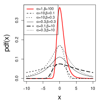
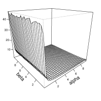
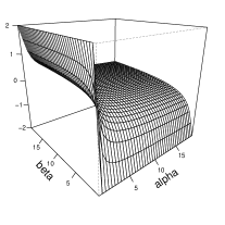
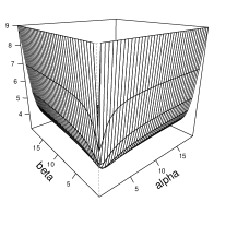
Figure 7: Density function and .99 quantile - GLIV$(0,1,\alpha,\beta)$; skewness and kurtosis - GLIV$(\mu,\sigma,\alpha,\beta)$

Prentice (1976) presents a simplified form of this distribution. When $\alpha=\beta$, the type IV generalized logistic distribution is symmetric about $x=\mu$, and the distribution is known as the type III generalized logistic distribution.

Exponentiated generalized Gumbel distribution.

Cordeiro et al. (2013) defined a class of distributions known as the exponentiated generalized distribution (EG), by

$$F(x)=[1-\{1-G(x)\}^{\alpha}]^{\beta},$$

where $\alpha>0$ and $\beta>0$ are two additional shape parameters and $G(x)$ is a continuous cdf. When $G(x)$ is the Gumbel cdf, EG becomes the exponentiated generalized Gumbel distribution (EGGu). Let $X\sim{\rm EGGu}(\mu,\sigma,\alpha,\beta)$ be an exponentiated generalized Gumbel distributed random variable with cdf

$$F_{{\rm EGGu}}(x;\mu,\sigma,\alpha,\beta)=\left[1-\left(1-\exp\left(-\exp\left(-\frac{x-\mu}{\sigma}\right)\right)\right)^{\alpha}\right]^{\beta},\quad x\in I\!\!R,$$

where $\alpha>0$ and $\beta>0$. The Gumbel distribution is a particular case of EGGu when $\alpha=\beta=1$ and the aforementioned exponentiated Gumbel distribution EGu is a special case when $\beta=1$. Note that, if $X\sim{\rm EGGu}(\mu,\sigma,1,\beta)$, then

$$F_{{\rm EGGu}}(x;\mu,\sigma,1,\beta)=\exp(-\exp(-(x-(\mu+\sigma\ln\beta))/\sigma))=F_{{\rm EGGu}}(x;\mu^{*},\sigma,1,1)=F_{{\rm EV}}(x;\mu^{*},\sigma),$$

where $\mu^{*}=\mu+\sigma\ln\beta$. Hence, the exponentiated Gumbel family of distributions EGGu$(\mu,\sigma,\alpha,\beta)$ where $\mu\in I\!\!R$, $\sigma>0$, $\alpha>0$ and $\beta>0$, is nonidentifiable. It coincides with the Gumbel family of distributions EV$(\mu^{*},\sigma)$, where $\mu^{*}\in I\!\!R$ and $\sigma>0$, when $\alpha=1$. Therefore, this distribution will not be considered further.

Beta Gumbel distribution.

Nadarajah & Kotz (2004) proposed a generalization of the Gumbel distribution, which they referred to as the beta Gumbel distribution (BG), from a generalized class of distributions defined by

$$F(x)=\frac{B_{G(x)}(\alpha,\beta)}{B(\alpha,\beta)},$$

for $\alpha>0$ and $\beta>0$, where $G(x)$ is a cdf, $B(\alpha,\beta)$ is the beta function and

$$B_{w}(a,b)=\int_{0}^{w}t^{a-1}(1-t)^{b-1}dt$$

is the incomplete beta function, by taking $G(x)$ as the Gumbel cdf.

Let $X\sim{\rm BG}(\mu,\sigma,\alpha,\beta)$ be a beta Gumbel distributed random variable with cdf

$$F_{{\rm BG}}(x;\mu,\sigma,\alpha,\beta)=\frac{1}{B(\alpha,\beta)}\int_{0}^{\exp(-\exp(-(x-\mu)/\sigma))}t^{\alpha-1}(1-t)^{\beta-1}dt,\quad x\in I\!\!R,$$

where $\alpha>0$ and $\beta>0$. When $\alpha=1$ and $\beta=1$, the beta Gumbel distribution reduces to a Gumbel distribution, and it reduces to an exponentiated Gumbel distribution (EGu) when $\alpha=1$.

If $X\sim{\rm BG}(\mu,\sigma,\alpha,1)$, then

$$F_{{\rm BG}}(x;\mu,\sigma,\alpha,1)=\alpha\int_{0}^{\exp(-\exp(-(x-\mu)/\sigma))}t^{\alpha-1}dt=F_{{\rm BG}}(x;\mu^{*},\sigma,1,1)=F_{{\rm EV}}(x;\mu^{*},\sigma),$$

where $\mu^{*}=\mu+\sigma\ln\alpha$. Therefore the beta Gumbel family of distributions BG$(\mu,\sigma,\alpha,\beta)$ with $\mu\in I\!\!R$, $\sigma>0$, $\alpha>0$ and $\beta>0$ is nonidentifiable. It coincides with the Gumbel family of distributions EV$(\mu^{*},\sigma)$ with $\mu^{*}\in I\!\!R$ and $\sigma>0$, when $\beta=1$. Therefore, this distribution will not be studied hereafter.

Kummer beta generalized Gumbel distribution.

Pescim et al. (2012) defined a class of distributions known as the Kummer beta generalized family (KBG). From an arbitrary cdf $G(x)$, the KGB family of distributions is defined by

$$F(x)=K\int_{0}^{G(x)}t^{\alpha-1}(1-t)^{\beta-1}\exp(-\gamma t)dt,$$

where $\alpha>0$, $\beta>0$ and $\gamma\in I\!\!R$ are shape parameters and

$$K^{-1}=\frac{\Gamma(a)\Gamma(b)}{\Gamma(a+b)}\;_{1}F_{1}(a;a+b;-c),$$

where ${}_{1}F_{1}(a;a+b;-c)=\sum_{k=0}^{\infty}[(a)_{k}(-c)_{k}]/[(a+b)_{k}k\;!]$ is the confluent hypergeometric function, $(d)_{k}=d(d+1)...(d+k-1)$ denotes the ascending factorial, and $(d)_{0}=1$. When $G(x)$ is a Gumbel cdf, it is known as the KGB-Gumbel distribution (KGBGu).

Let $X\sim{\rm KBGGu}(\mu,\sigma,\alpha,\beta,\gamma)$ be a KGB-Gumbel distributed random variable with cdf

$$F_{{\rm KBGGu}}=K\int_{0}^{\exp(\exp(-(x-\mu)/\sigma))}t^{\alpha-1}(1-t)^{\beta-1}\exp(-\gamma t)dt,$$

where $\alpha>0$, $\beta>0$ and $\gamma\in I\!\!R$. When $\alpha=1$, $\beta=1$ and $\gamma=0$, the KGB-Gumbel distribution reduces to the Gumbel distribution and it reduces to a beta Gumbel distribution when $\gamma=0$.

If $X\sim{\rm KBGGu}(\mu,\sigma,\alpha,1,0)$, then

$$F_{{\rm KBGGu}}(x;\mu,\sigma,\alpha,1,0)=\alpha\int_{0}^{\exp(-\exp(-(x-\mu)/\sigma))}t^{\alpha-1}dt=F_{{\rm KBGGu}}(x;\mu^{*},\sigma,1,1,0)=F_{{\rm EV}}(x;\mu^{*},\sigma),$$

where $\mu^{*}=\mu+\sigma\ln\alpha$. Hence, the Kummer beta Gumbel family of distributions KBGGu$(\mu,\sigma,\alpha,\beta,\gamma)$ with $\mu\in I\!\!R$, $\sigma>0$, $\alpha>0$, $\beta>0$ and $\gamma\in I\!\!R$ is nonidentifiable. It coincides with the Gumbel family distributions EV$(\mu^{*},\sigma)$ with $\mu^{*}\in I\!\!R$ and $\sigma>0$, when $\beta=1$ and $\gamma=0$. Therefore, this distribution will not be examined in the following discussion.

Two-component extreme value distribution (TCEV).

In studying annual flood series, Rossi et al. (1984) considered an approach to account for both the presence of outliers and high skewness. That approach results from assuming that flood peaks do not all arise from one and the same distribution but, instead, from a two-component extreme value mixture (TCEV). One of the components generates ordinary (more frequent and less severe in the mean) floods. The other exhibits much greater variability and tends to generate more rare but more severe floods.

Let $X\sim{\rm TCEV}(\mu,\sigma,\mu_{1},\sigma_{1},\alpha)$ be a two-component extreme value distributed random variable. Its pdf and cdf are, respectively,

$$f_{{\rm TCEV}}(x;\mu,\sigma,\mu_{1},\sigma_{1},\alpha) = \frac{1-\alpha}{\sigma}\exp\left(-\frac{x-\mu}{\sigma}\right)\exp\left(-\exp\left(-\frac{x-\mu}{\sigma}\right)\right)$$

$$+\frac{\alpha}{\sigma_{1}}\exp\left(-\frac{x-\mu_{1}}{\sigma_{1}}\right)\exp\left(-\exp\left(-\frac{x-\mu_{1}}{\sigma_{1}}\right)\right),\;\;x\in I\!\!R,$$

and

$$F_{{\rm TCEV}}(x;\mu,\sigma,\mu_{1},\sigma_{1},\alpha) = (1-\alpha)\exp\left(-\exp\left(-\frac{x-\mu}{\sigma}\right)\right)$$

$$+\alpha\exp\left(-\exp\left(-\frac{x-\mu_{1}}{\sigma_{1}}\right)\right),\;\;x\in I\!\!R,$$

where $\mu\in I\!\!R$ and $\mu_{1}\in I\!\!R$ are location parameters, $\sigma>0$ and $\sigma_{1}>0$ are dispersion parameters and $0<\alpha<1$. Greater values of $\alpha$ increase the weight of the second component.

If $0<\alpha<1$, $F(x;\mu,\sigma,\mu_{1},\sigma_{1},\alpha)=F(x;\mu_{1},\sigma_{1},\mu,\sigma,(1-\alpha))$, then consequently, the mixture is nonidentifiable. The lack of identifiability due to the label-switching effect is overcome by imposing identifiability constraints on the parameters. It is sufficient to consider $0<\alpha<0.5$ to achieve identifiability. When $\alpha\rightarrow 0$, the two-component extreme value distribution reduces to a Gumbel distribution.

Data from $X\sim{\rm TCEV}(\mu,\sigma,\mu_{1},\sigma_{1},\alpha)$ may be generated from the conditional distributions $X|Z=0\sim EV(\mu,\sigma)$ and $X|Z=1\sim EV(\mu_{1},\sigma_{1})$, where $Z\sim{\rm Bernoulli}(\alpha)$.

Figure 8 shows the plots of the pdf for selected parameters, and the .99 quantile, skewness and kurtosis of TCEV$(0,1,10,5,\alpha)$. Note that the probability of high values of the random variable and the $.99$ quantile grow with $\alpha$. The skewness and kurtosis coefficients are smaller than the corresponding Gumbel values for all $\alpha$.

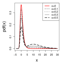
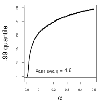
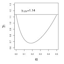
Figure 8: Density function, .99 quantile, skewness and kurtosis - TCEV$(0,1,10,5,\alpha)$

As a summary, Table 1 presents the generalizations of the Gumbel presented above; the nonidentifiable distributions are marked with an asterisk. In the following sections, we will consider all the identifiable family of distributions, namely EV, GEV, EGu, TEV, GTIEV3, EGa, GGu, GLIV, and TCEV.

Table 1: Generalizations of the Gumbel distribution.

Distribution	Proposed by
Generalized extreme value GEV($\mu,\sigma,\alpha$)	Jenkinson (1955)
Type IV generalized logistic GLIV($\mu,\sigma,\alpha$)	Prentice (1975)
Two-component extreme value TCEV($\mu,\sigma,\mu_{1},\sigma_{1},\alpha$)	Rossi et al. (1984)
Three parameter exponential-gamma EGa($\mu,\sigma,\alpha$)	Ojo (2001)
Exponentiated Gumbel EGu($\mu,\sigma,\alpha$)	Nadarajah (2006)
Transmuted extreme value TEV($\mu,\sigma,\alpha$)	Aryal & Tsokos (2009)
Generalized Gumbel GGu($\mu,\sigma,\alpha$)	Cooray (2010)
Generalized three-parameter Gumbel GTIEV3($\mu,\sigma,\alpha$)	Jeong et al. (2014)
Generalized type I extreme value GTIEV($\mu,\sigma,\alpha,\beta$) ∗	Dubey (1969)
Exponential-gamma ExpGamma($\mu,\sigma,\alpha,\beta$) ∗	Adeyemi & Ojo (2003)
Beta Gumbel BG($\mu,\sigma,\alpha,\beta$) ∗	Nadarajah & Kotz (2004)
Kummer beta generalized Gumbel KBGGu($\mu,\sigma,\alpha,\beta,\gamma$) ∗	Pescim et al. (2012)
Kumaraswamy Gumbel KumGum($\mu,\sigma,\alpha,\beta$) ∗	Cordeiro et al. (2012)
Exponentiated generalized Gumbel EGGu($\mu,\sigma,\alpha,\beta$) ∗	Cordeiro et al. (2013)

3 Right-tail heaviness

Heavy right-tailed distributions have been used to model phenomena in economics, ecology, bibliometrics, and biometry, among others; see, for instance, Markovich (2007) and Resnick (2007). We next describe two criteria used to evaluate the right-tail heaviness of a distribution.

Informally, a regular variation function is asymptotically equivalent to a power function. Formally, a Lebesgue measurable function $U:I\!\!R^{+}\rightarrow I\!\!R^{+}$ is regularly varying at infinity with index $\rho$ ($U\in RV_{\rho}$ ), if $\lim\limits_{t\to\infty}U(tx)/U(t)=x^{\rho}$, for $x>0$. If $\rho=0$, $U$ is referred to as slowly varying. The function $U$ varies rapidly at infinity (or is rapidly varying at infinity with index $\infty$ ($-\infty$), or $U\in RV_{\infty}$ ($U\in RV_{-\infty}$) (de Haan, 1970, p. 4), if $\forall x$

$$\begin{matrix}\lim\limits_{t\rightarrow\infty}\frac{U(tx)}{U(t)}:=x^{\infty}=\left\{\begin{matrix}0&{\rm if}&0<x<1\\ 1&{\rm if}&x=1\\ \infty&{\rm if}&x>1.\end{matrix}\right.&\left(\lim\limits_{t\rightarrow\infty}\frac{U(tx)}{U(t)}:=x^{-\infty}=\left\{\begin{matrix}\infty&{\rm if}&0<x<1\\ 1&{\rm if}&x=1\\ 0&{\rm if}&x>1.\end{matrix}\right.\right).\end{matrix}$$

A distribution with cdf $F$ is said to have a heavy right tail whenever the survival function, $\overline{F}:=1-F$, is a regularly varying at infinity function with a negative index of regular variation $\rho=-1/\xi,\;\xi>0$, i.e., $\lim\limits_{t\rightarrow\infty}\overline{F}(tx)/\overline{F}(t)=x^{-1/\xi}$. The parameter $\xi$ is known as the tail index, and is one of the primary parameters of rare events. The distribution is said to have light (non-heavy) right tail if the limit equals $x^{-\infty}$, and $\xi=0$. When the limit equals 1, i.e. $\overline{F}$ is a slowly varying function, we will say that the distribution has a heavy right tail with tail index $\xi=\infty$. It follows from de Haan (1970, Corollary 1.2.1 - 2 and 3) that the index of regular variation is invariant under the location-scale transformation. It is thus sufficient to derive it from the standard form of the distribution.

The generalized extreme value distribution GEV($\mu,\sigma,\alpha$) has a heavy right tail with tail index $\alpha$ when $\alpha>0$ (Fréchet family). It has a non-heavy right tail when $\alpha=0$ (Gumbel family). Other heavy right-tailed distributions are, e.g., Student-t($\nu$) ($\xi=1/\nu$), Cauchy ($\xi=1$) and F($\alpha,\beta$) ($\xi=2/\beta$). The other distributions addressed in this paper, viz., Gumbel (EV), exponentiated Gumbel (EGu), transmuted extreme value (TEV), generalized three-parameter Gumbel (GTIEV3), three-parameter exponential-gamma (EGa), type IV generalized logistic (GLIV), generalized Gumbel distribution (GGu), and two-component extreme value distribution (TCEV), are all non-heavy right-tailed distributions (see Supplement). Hence, among the identifiable distributions addressed in this work, the GEV distribution is the only one with a potentially heavier right tail than that of the Gumbel distribution under the tail index approach.

Rigby et al. (2014) ordered the heaviness of the tails of a continuous distribution based on the logarithm of the pdf. If random variables $X_{1}$ and $X_{2}$ have continuous pdf $f_{X_{1}}(x)$ and $f_{X_{2}}(x)$ and $\lim\limits_{x\to\infty}f_{X_{1}}(x)=\lim\limits_{x\to\infty}f_{X_{2}}(x)=0$, then $X_{2}$ has a heavier right tail than $X_{1}$ if and only if $\lim\limits_{x\to\infty}[\ln f_{X_{2}}(x)-\ln f_{X_{1}}(x)]=\infty$. There are three main forms for $\ln f_{X}(x)$ when $x\to\infty$ (right tail) or $x\to-\infty$ (left tail): $\ln f_{X}(x)\approx-k_{2}(\ln|x|)^{k_{1}}$ (type I), $\ln f_{X}(x)\approx-k_{4}|x|^{k_{3}}$ (type II) or $\ln f_{X}(x)\approx-k_{6}\exp(k_{5}|x|)$ (type III). The three types are in decreasing order of tail heaviness. For type I, decreasing $k_{1}$ results in a heavier tail while decreasing $k_{2}$ for fixed $k_{1}$ results in a heavier tail. Similarly, for the two types. If two distributions have the same values of $k_{1}$ and $k_{2}$ (analogously for $k_{3}$ and $k_{4}$, or $k_{5}$ and $k_{6}$), their right tails are not necessarily equally heavy. In this case, it is necessary to compare the second-order terms of the logarithm of the pdf to distinguish the distributions.

Table 2 summarizes the right tail asymptotic form of the logarithm of the pdf for the distributions mentioned above. The GEV distribution with $\alpha>0$ is of type I with $k_{1}=1$ and $k_{2}=1+1/\alpha$. As expected, the GEV distribution is the only one that has a ‘Paretian type’ right tail (type I with $k_{1}=1$ and $k_{2}>1$). Note that the Cauchy distribution has $k_{1}=1$ and $k_{2}=2$, and hence if $\alpha>1$, the GEV distribution has a heavier right tail than that of the Cauchy distribution. The Student-t distribution with $\nu$ degrees of freedom has $k_{1}=1$ and $k_{2}=1+\nu$. If $\alpha>1/2$, the right tail heaviness of the GEV distribution is greater than that of the Student-t distribution with two degrees of freedom, which is uncommon in real data.

The Gumbel distribution is of type II with $k_{3}=1$ and $k_{4}=1/\sigma$. According to Rigby et al. (2014), distributions with $k_{3}=1$ are non-heavy tailed. All of the other distributions are also of type II and non-heavy tailed distributions. The EGu, EGa, GGu, and GLIV distributions have $k_{4}=\alpha/\sigma$, and hence they have heavier right tail than the Gumbel distribution when $\alpha<1$. The TEV, GTIEV3, and TCEV distributions have the same $k_{4}=1/\sigma$ as the Gumbel distribution. To distinguish among the TEV, GTIEV3 and TCEV distributions it is necessary to compare the second-order terms of the logarithm of their pdf. Comparing the second-order terms, the TEV distribution with $\alpha<0$ and the TCEV distribution have heavier right tail than the Gumbel distribution. The right tail of the GTIEV3 distribution is lighter than that of the Gumbel distribution (see Supplement). These findings agree with the pdf plots shown in Figures 3, 4, and 8, respectively.

Table 2: Right tail asymptotic form of the logarithm of the pdf for the Gumbel distribution and its generalizations

[c] GEV EGu EGa GLIV GGu EV GTIEV3 TEV TCEV parameter $\alpha>0$ $\alpha>0$ $\alpha>0$ $\alpha>0$ $\alpha>0$ $\alpha>0$ $-1<\alpha\leq 1$ $0<\alpha<0.5$ $k_{1}$ 1 $\alpha>0$ $k_{2}$ $1+1/\alpha$ $k_{3}$ 1 1 1 1 1 1 1 1 $k_{4}$ $\alpha/\sigma$ $\alpha/\sigma$ $\alpha/\sigma$ $\alpha/\sigma$ $1/\sigma$ $1/\sigma$ $1/\sigma$ $1/\sigma_{2}$ ^*

• if $\sigma_{1}<\sigma_{2}$.

4 Monte Carlo simulation results

We next compare the ability of the Gumbel distribution and its generalizations to model data taken from different distributions. To this end, we present a Monte Carlo simulation study in which 10,000 samples of size 500 are generated from and modeled with each of the identifiable distributions considered in this paper. For generating the data, we set $\mu=0$ and $\sigma=1$ (for the TCEV distribution $\mu_{1}=10$ and $\sigma_{1}=5$). The remaining parameters were chosen in such a way that the $.999$ quantile is close to 10 whenever possible. Table 3 presents the distributions from which the samples were drawn and their $.999$ quantile and kurtosis.

Table 3: Distributions, $.999$ quantile, and kurtosis

	EV	GEV	EGu	TEV	EGa	GGu	GLIV	TCEV
Parameters	$-$	$\alpha=0.1$	$\alpha=0.7$	$\alpha=-0.99$	$\alpha=0.7$	$\alpha=0.7$	$\alpha=0.65$	$\alpha=0.0016$
							$\beta=15$	$\mu_{1}=10$, $\sigma_{1}=5$
$x_{.999}$	6.91	9.95	9.87	7.60	9.99	9.87	10.38	10.28
Kurtosis	5.40	10.98	6.28	5.39	6.22	5.72	6.26	5.38

As measures of model adequacy, we use the Akaike information criterion (AIC) and two modified Anderson Darling statistics (ADR and AD2R). AIC is a measure of dissimilarity between two distributions over the support; smaller AIC suggests that the fit is closer to the true density. ADR and AD2R (Luceño, 2005, Table 2 and B.1) are sensitive to the lack of fit in the right tail of the distribution. AD2R puts more weight in the right tail than ADR. Smaller values of ADR and AD2R are indicative of a better fit.

A characteristic that is often of interest in extreme data modeling is the return level. The return level with return period $1/p$ is the quantile $x_{1-p}$, and it is interpreted as the value that we expect to be exceeded once every $1/p$ periods on average. To evaluate the quantile goodness of fit, we compute the $.999$ quantile discrepancy, which is defined as the difference between the $.999$ quantile of the fitted model and the $.999$ quantile of the distribution from which samples are generated divided by the latter.

The estimates of the parameters were obtained by numerically maximizing the log-likelihood function. For the maximization procedure, we used a method that implements a sequential quadratic programming technique to maximize a nonlinear function subject to non-linear constraints, similar to Algorithm 18.7 in Wright & Nocedal (1999). This method is implemented in the function MaxSQP in the matrix programming language Ox (Doornik, 2013) and allows to establish bounds for the individual parameters. For the TEV distribution, we used the profile log-likelihood function for the parameter $\alpha$. We used the bounds $-0.6<\alpha<0.6$, for the GEV distribution, and $0<\alpha<1$ and $0<\beta<20$, for the GLIV distribution. The GTIEV3 distribution is not included in the simulation study because it behaves like the EV distribution with respect to the right tail.

Figures 9 and 10 present the boxplots of AIC, ADR, AD2R, and the .999 quantile discrepancies of the fitted models. For these figures, the samples were generated from the EV($0,1$) and the GEV($0,1,0.1$) distributions, respectively. The figures, corresponding to the cases where the samples were generated from the EGu($0,1,0.7$), TEV($0,1,-0.99$), EGa($0,1,0.7$), GGu($0,1,0.7$), GLIV($0,1,0.65,15$) and TCEV($0,1,10,5,0.0016$) distributions, are presented in the Supplement. For the GEV distribution, we show results for two estimation methods: maximum likelihood estimation (GEV-MLE) and probability-weighted moments (GEV-PWM) methods (Castillo et al., 2005, Section 5.3).

For the Gumbel distributed samples (Figure 9), the boxplots of AIC are quite similar and suggest that all generalizations of the Gumbel distribution can suitably fit Gumbel distributed data. The goodness of fit at the right tail, illustrated by the boxplots of ADR, are also quite similar except for the Gumbel and the GLIV distributions. For the Gumbel distribution, the median and the dispersion are bigger than for the other distributions. The GLIV fit is poor in the right tail, which is consistent with the quantile plot in Figure 7, that suggests that a small difference in the estimated parameter $\alpha$ produces a significant difference in the upper quantiles. This characteristic makes the right tail goodness of fit dependent on the precision adopted for the parameter estimation. Boxplots of AD2R emphasize the right-tail lack of fit. The boxplots of AD2R in Figure 9 are similar except for the GLIV fit, whose interquartile range (IQR) is the largest. The GEV-MLE right tail fit seems to be slightly better than the others. The boxplots of $0.999$ quantile discrepancy show that the median is close to zero for all the distributions. The EV and GGu fits exhibit the smallest amplitudes. The TEV fit presents some cases of marked underestimation due to numerical problems.

Figure 9: Boxplots of AIC (first row), ADR (second row), AD2R (third row) and .999 quantile discrepancies (fourth row) - random samples generated from EV.

For the GEV distributed samples (Figure 10), the boxplots of AIC of the EV and TEV fits present the biggest medians, and the GEV-MLE, GEV-PWM, and TCEV fits exhibit the smallest amplitudes. We recall that, theoretically, the AIC of the GEV-MLE fit can not be bigger than that of the GEV-PWM fit. The boxplots of ADR and AD2R highlight the GEV-PWM fit as the best right-tail fit. The boxplots of quantile discrepancy show that the GEV-PWM and GEV-MLE fits have the closest to zero medians, and all the others underestimate the $.999$ quantile, markedly the EV and TEV fits.

Figure 10: Boxplots of AIC (first row), ADR (second row), AD2R (third row) and .999 quantile discrepancies (fourth row) - Random samples generated from GEV.

Hereafter we analyze the fits when the data were generated from the other distributions (see boxplots in the Supplement). The boxplots of AIC are similar to those in Figure 9. The boxplots of ADR for the TCEV fit exhibit the smallest medians and IQR followed by the GEV-PWM fit except for samples generated from the TCEV distribution when it is followed by the EGu, EGa, and GEV-MLE fits. The boxplots of AD2R reveal that the GEV-MLE fit is among the best fits regardless of from which distribution the data were generated. When generating the data from the GLIV distribution, all the distributions underestimate the $.999$ quantile, and this is the only case where the GEV-MLE and GEV-PWM fits underestimate the $.999$ quantile.

Summing up, the GEV-PWM, TCEV, and GEV-MLE fits are among the best fits in all of the simulated settings.

5 Application to a wind speed data set

We analyze data on the maximum monthly peak gust wind speed (mph) in West Palm Beach, Florida (USA) for the months January, 1984 to November, 2014, with $n=371$ observations. The data are available online for download from the National Climate Data Center (NCDC) – National Oceanic and Atmospheric Administration (NOAA) at http://www.ncdc.noaa.gov/ and given in the Supplement. We fit the different models described in Section 2 to the seasonally adjusted wind speed data. The seasonally adjusted wind speed was calculated removing the seasonal component using a robust seasonal trend decomposition implemented in the functions stl of the R package stats and seasadj of the package forecast (Cleveland et al., 1990). The maximum likelihood estimates of the parameters were obtained similarly as in the Monte Carlo simulation (Section 4).

Figure 11 shows the scatterplot, the adjusted boxplot for asymmetric distributions (Hubert & Vandervieren, 2008) and the histogram of the data together with the fitted densities. The outliers at the right tail of the adjusted boxplot are much more spread than those at the left one. The empirical skewness and kurtosis coefficients are 2.26 and 13.42, respectively. Both are much higher than those expected from a Gumbel distribution (1.14 and 5.4, respectively), which suggests the fitting of the generalized distributions. Recall that the only distribution for which the skewness can be higher than 2 and the kurtosis can be higher than 9 is the GEV distribution.

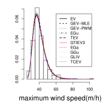
Figure 11: Scatterplot, boxplot, adjusted boxplot, and histogram; wind speed data.

The maximum likelihood estimates and the probability weighted moments estimates for the GEV distribution (standard errors in parentheses) and the estimated return levels of the seasonally adjusted series of the return period of one thousand months from the selected distributions are summarized in Table 4. The additional parameter $\alpha$ estimate of the GTIEV3 distribution is notably high, i.e., the fitted GTIEV3 distribution nearly coincides with the fitted Gumbel distribution. Recall that the Gumbel distribution is a limiting case of the GTIEV3 distribution when $\alpha\to\infty$. Indeed, estimates of $\mu$ and $\sigma$ for these distributions are the same up to the third decimal places. The estimated return levels of a return period of one thousand months (for the seasonally adjusted data) from the selected distributions differ by up to 20 mph. The Gumbel distribution produces the smallest estimated return level (77.23 mph), and the largest estimates are obtained from the GEV-PWM (89.52 mph) and TCEV (100.21 mph) fits.

Table 4: Parameter estimates, standard errors (in parentheses) and return level for a thousand years - wind speed data.

	$\hat{\mu}$	$\widehat{\sigma}$	$\widehat{\alpha}$	$\widehat{\beta}$ or $\widehat{\mu_{1}}$	$\widehat{\sigma_{1}}$	$\widehat{x_{.999}}$
EV	36.94(0.32)	5.83(0.24)	–	–	–	77.23
GEV-MLE	36.75(0.34)	5.72(0.25)	0.06(0.03)	–	–	85.74
GEV-PWM	36.67(0.34)	5.53(0.25)	0.09(0.03)	–	–	89.52
EGu	35.78(0.95)	5.07(0.63)	0.79(0.16)	–	–	80.34
TEV	39.19(0.35)	6.95(0.29)	0.61(0.16)	–	–	80.57
GTIEV3	36.94(0.29)	5.83(0.22)	16698.18(-)	–	–	77.23
EGa	35.10(1.24)	4.89(0.68)	0.75(0.16)	–	–	80.83
GGU	36.89(0.38)	6.07(0.43)	1.03(0.11)	–	–	77.69
GLIV	36.67(0.48)	2.94(1.00)	0.43(0.17)	2.16(1.95)	–	81.98
TCEV	36.70(0.37)	5.51(0.30)	0.02(0.02)	61.56(23.41)	13.38(8.22)	100.21

Figure 12 displays the profile log-likelihood function for the additional parameter(s) of the fitted models. The profile log-likelihood function is well behaved if there is no inflection point, multimodality or lack of concavity. Note the slight concavity in the profile log-likelihood function for the EGu, EGa, and GGu models. The profile log-likelihood function for the TEV model exhibits an inflection point, a local minimum, and two local maxima, and hence maximization can converge to a local maximum depending on the initial value. The profile log-likelihood function for the GTIEV3 model is increasing and flat for large values of $\alpha$. Hence, the estimate of $\alpha$ depends on the numerical precision specified for the maximization algorithm, and the standard error estimate is very large. The profile log-likelihood function for the GLIV model also varies slowly in the $\beta$ parameter direction. The profile log-likelihood function for the TCEV model presents inflection points. This appears not to disturb the parameter estimation because of the highly concave profile log-likelihood function near its maximum. The profile log-likelihood function for the GEV model is well behaved.

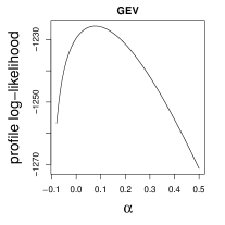
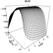
Figure 12: Profile log-likelihood function - wind speed data.

A summary of the goodness of fit measures is given in Table 5. The GEV-MLE, GEV-PWM, TEV, GLIV, and TCEV fits produce smaller AIC and ADR measures than the EV fit. The AD2R measure highlights the EV and the GTIEV3 fits (235.75 and 235.82, respectively) as the worst fits. It points to the TCEV (2.33) and the GEV-PWM (7.13) as the best fits. All the goodness of fit measures reveal that the Gumbel distribution is not the best choice for this data set. Taking all of the goodness of fit criteria into account, we conclude that the GEV and TCEV distributions produce the best fits.

Table 5: Goodness of fit measures - wind speed data.

	EV	GEV	GEV	EGu	TEV	GTIEV3	EGa	GGu	GLIV	TCEV
		MLE	PWM
$-\ell(\widehat{\theta})$	1245.08	1242.98	1243.69	1244.34	1242.59	1245.08	1244.23	1245.20	1243.04	1241.24
AIC	2494.15	2491.96	2493.39	2494.67	2491.18	2496.15	2494.47	2496.40	2494.08	2492.47
ADR	0.58	0.46	0.39	0.55	0.37	0.58	0.54	0.65	0.35	0.31
AD2R	235.75	15.84	7.13	91.88	70.75	235.82	84.84	205.59	56.41	2.33

Figure 13 shows the qqplots of the fitted models. As an aid to interpretation, envelopes were generated by simulation. The envelopes correspond to pointwise two-sided 90% confidence intervals with the bootstrap replicates of each curve generated from the fitted model. The qqplots for the Gumbel, EGu, TEV, GTIEV3, EGa, GGu, and GLIV distributions clearly suggest a lack of fit at the extreme of the right tail. However, the qqplots for the GEV (both estimation methods, MLE and PWM) and TCEV distributions accommodate all of the observations of the right tail inside the envelope. Therefore, qqplots corroborate the previous conclusions that the GEV and TCEV models provide the best fits for this data set.

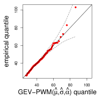
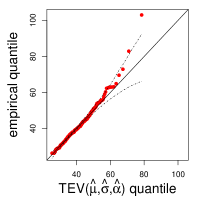
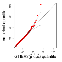
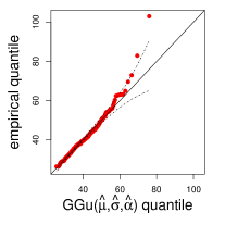
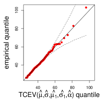
Figure 13: QQplots - wind speed data.

6 Conclusion

Motivated by real problems with a probability of extreme events that is larger than usual, we investigated distributions that generalize the Gumbel extreme value distribution, frequently used to model extreme value phenomena. We showed that some generalized Gumbel distributions proposed in the literature are nonidentifiable, which limits their usefulness in applications. We gathered the moments, quantiles, generating data methods, skewness and kurtosis coefficients, and classified their right-tail heaviness according to two criteria. We provided a simulation study to evaluate the capacity of the selected distributions to fit data with kurtosis larger than that of the Gumbel distribution. Our simulation results revealed that the generalized extreme value (GEV) distribution is more flexible in fitting this type of data and that the two-component extreme value (TCEV) distribution can also be a good choice. An application to an extreme wind speed data set in Florida confirmed the simulation study, with the GEV and TCEV models providing better fits than the other distributions.

As indicated by our simulations, practitioners should consider the GEV and TCEV distributions to model extreme value data with a heavy right tail.

Supplement

A comparative review of generalizations of
the Gumbel extreme value distribution
with an application to wind speed data

1 Moments and quantiles

The skewness ($\gamma_{1}$) and kurtosis ($\gamma_{2}$) coefficients of the distributions are obtained from the central moments (E($(X-{\rm E}(X))^{n}$)) or the moments (E($X^{n}$)), and the equations

$$\gamma_{1}=\frac{{\rm E}((X-{\rm E}(X))^{3})}{[{\rm E}((X-{\rm E}(X))^{2})]^{3/2}}=\frac{{\rm E}(X^{3})-3{\rm E}(X){\rm E}(X^{2})+2{\rm E}(X)^{3}}{({\rm E}(X^{2})-{\rm E}(X)^{2})^{3/2}},$$

$$\gamma_{2}=\frac{{\rm E}((X-{\rm E}(X))^{4})}{[{\rm E}((X-{\rm E}(X))^{2})]^{2}}=\frac{{\rm E}(X^{4})-4{\rm E}(X){\rm E}(X^{3})+6{\rm E}(X)^{2}{\rm E}(X^{2})+3{\rm E}(X)^{4}}{({\rm E}(X^{2})-{\rm E}(X)^{2})^{2}}.$$

For the GEV distribution, we used that

$$\int_{0}^{\infty}x^{\nu-1}\exp(-\mu x)dx=1/\mu^{\nu}\Gamma(\nu),$$

if Re $\mu>0$ and Re $\nu>0$ (Gradshteyn & Ryzhik, 2000, equation 3.381.4).

For the standard EGu distribution, the moment of order $n$ is

$${\rm E}(X^{n})=\int_{0}^{\infty}\alpha(-\ln(-\ln y))^{n}\;_{2}F_{1}(1-\alpha,1,1,y)dy.$$

For each value of $\alpha$, the $n$-th moment can be obtained by numerical integration with the computer algebra software Mathematica (Wolfram Research, 2012) as follows:

Clear[a];Clear[EX1];Clear[EX2];Clear[EX3];Clear[EX4];
Clear[skewness];Clear[kurtosis];
EX1:=-a*NIntegrate[(Log[-Log[y]])^1*Hypergeometric2F1[(1-a),1,1,y],{y,0,1}]
EX2:=a*NIntegrate[(Log[-Log[y]])^2*Hypergeometric2F1[(1-a),1,1,y],{y,0,1}]
EX3:=-a*NIntegrate[(Log[-Log[y]])^3*Hypergeometric2F1[(1-a),1,1,y],{y,0,1}]
EX4:=a*NIntegrate[(Log[-Log[y]])^4*Hypergeometric2F1[(1-a),1,1,y],{y,0,1}]
a:=Table[i/100,{i,200}]
skewness=(EX3-3*EX2*EX1+2*EX1^3)/(EX2-EX1^2)^(3/2)//N
Clear[a];a := Table[i/100, {i, 300}]
kurtosis = (EX4 - 4*EX3*EX1 + 6*EX2*EX1^2 - 3*EX1^4)/(EX2 - EX1^2)^2//N

For the TEV distribution, we used the moments in Aryal & Tsokos (2009, p. 1404). For the EGa distribution, we used that

$$\int_{0}^{\infty}x^{\nu-1}\exp(-\mu x)(\ln x)^{n}dx=\partial^{n}(\mu^{-\nu}\Gamma(\nu))/\partial\nu^{n},$$

for $n=0,1,2,3,\ldots$ (Gradshteyn & Ryzhik, 2000, equation 4.358.5), where $\Gamma(x)=\int_{0}^{\infty}\exp(-t)t^{x-1}dt$ and ${\rm Re}\;x>0$ is the Gamma function. For the GLIV distribution, we used its moment generating function. For the GGu distribution, the central moment of order $n$ is

$${\rm E}((X-{\rm E}(X))^{n})=\int_{0}^{\infty}\left(-\sigma\left(\ln\ln(1+y^{-1/\alpha})+{\mathcal{E}}(1,\alpha)\right)\right)^{n}(1+y)^{-2}dy,$$

where ${\mathcal{E}}(n,\alpha)=-\int_{0}^{\infty}(\ln\ln(1+y^{-1/\alpha}))^{n}(1+y)^{-2}dy$ and ${\mathcal{E}}(1,1)={\mathcal{E}}$ is the Euler’s constant. For each value of $\alpha$, the skewness and kurtosis can be obtained by numerical integration with the computer algebra software Mathematica (Wolfram Research, 2012) as follows:

Clear[alpha]; Clear[E1]; Clear[E2]; Clear[E3]; Clear[E4]
alpha = Table[i/10, {i, 7, 100}]
E1 = -NIntegrate[Log[Log[1 + x^(-1/alpha)]]/(1 + x)^2, {x, 0, Infinity}]
E2 = -NIntegrate[Log[Log[1 + x^(-1/alpha)]]^2/(1 + x)^2, {x, 0, Infinity}]
E3 = -NIntegrate[Log[Log[1 + x^(-1/alpha)]]^3/(1 + x)^2, {x, 0, Infinity}]
E4 = -NIntegrate[Log[Log[1 + x^(-1/alpha)]]^4/(1 + x)^2, {x, 0, Infinity}]
skewness = -(-E3 - 3 E2*E1 - 2 E1^3)/(-E2 - E1^2)^(3/2)
kurtosis = (-E4 - 4 E3*E1 - 6 E2*E1^2 - 3 E1^4)/(-E2 - E1^2)^2

Table 1 presents moments, skewness and kurtosis coefficients and quantile functions for the Gumbel distribution (EV) and its generalizations.

Table 1: Moments, skewness and kurtosis coefficients and quantile functions

[c] E($X$) var($X$) EV$(\mu,\sigma)$ $\mu+\sigma{\mathcal{E}}$ $\sigma^{2}\,\pi^{2}/6$ GEV$(\mu,\sigma,\alpha),\,\alpha\neq 0$ $\mu+(\sigma/\alpha)\left(\Gamma(1-\alpha)-1\right),\,\alpha<1$ $(\sigma/\alpha)^{2}\left(\Gamma(1-2\alpha)-\Gamma^{2}(1-\alpha)\right),\,2\alpha<1$ EGu$(\mu,\sigma,\alpha)$ $-$ $-$ TEV$(\mu,\sigma,\alpha)$ $(\mu+{\mathcal{E}}\sigma)-\alpha\sigma\ln 2$ $\sigma^{2}(\pi^{2}/6-\alpha(1+\alpha)(\ln 2)^{2})$ GTIEV3$(\mu,\sigma,\alpha)$ $\mu-\sigma(-\mathcal{E}+\ln(\alpha)-\psi(\alpha))$ ^I $\sigma^{2}(\pi^{2}/6+\psi^{\prime}(\alpha))$ ^II EGa$(\mu,\sigma,\alpha)$ $\mu-\sigma\psi(\alpha)$ $\sigma^{2}\psi^{\prime}(\alpha)$ GGu$(\mu,\sigma,\alpha)$ $\mu+\sigma{\mathcal{E}}(1,\alpha)$ $\sigma^{2}(-{\mathcal{E}}(2,\alpha)-{\mathcal{E}}^{2}(1,\alpha))$ GLIV$(\mu,\sigma,\alpha,\beta)$ $\mu+\sigma(\psi(\beta)-\psi(\alpha)-\ln(\beta/\alpha))$ $\sigma^{2}(\psi^{\prime}(\beta)+\psi^{\prime}(\alpha))$ TCEV$(\mu,\sigma,\mu_{1},\sigma_{1},\alpha)$ $(1-\alpha)(\mu+\sigma{\mathcal{E}})+\alpha(\mu_{1}+\sigma_{1}{\mathcal{E}})$ $(1-\alpha)\sigma^{2}\pi^{2}/6+\alpha\sigma_{1}^{2}\pi^{2}/6+$ $\alpha(1-\alpha)(\mu+\sigma{\mathcal{E}}-\mu_{1}-\sigma_{1}{\mathcal{E}})^{2}$ Quantile $x_{p}$ E($X^{n}$) EV$(\mu,\sigma)$ $\mu-\sigma\ln(-\ln(p))$ $\sum_{i=0}^{n}\genfrac{(}{)}{0.0pt}{}{n}{i}\mu^{n-i}\sigma^{i}(-1)^{i}\Gamma^{(i)}(1)$ ^III GEV$(\mu,\sigma,\alpha),\,\alpha\neq 0$ $\mu+(\sigma/\alpha)((-\ln(p))^{-\alpha}-1)$ $\left(\frac{1}{\alpha}\right)^{n}\sum_{i=0}^{n}\genfrac{(}{)}{0.0pt}{}{n}{i}\left(\mu\alpha-\sigma\right)^{n-i}\sigma^{i}\Gamma\bigl{(}1-\alpha i\bigr{)}$ EGu$(\mu,\sigma,\alpha)$ $\mu-\sigma\ln(-\ln(1-(1-p)^{1/\alpha}))$ $\alpha\sum_{i=0}^{n}\genfrac{(}{)}{0.0pt}{}{n}{i}\mu^{n-i}\sigma^{i}(-1)^{i}\int_{0}^{1}\left(\ln(-\ln y)\right)^{i}\;_{2}F_{1}(1-\alpha,1,1,y)dy$ TEV$(\mu,\sigma,\alpha)$ $\mu-\sigma\ln\left(-\ln\left((1+\alpha-\sqrt{(1+\alpha)^{2}-4\alpha p})/2\alpha\right)\right)$ $\sum_{i=0}^{n}\genfrac{(}{)}{0.0pt}{}{n}{i}\mu^{n-i}\sigma^{i}(-1)^{i}\Biggl{(}(1+\alpha)\Gamma^{(i)}(1)-2\alpha\frac{\partial^{i}}{\partial\nu^{i}}\biggl{[}2^{-\nu}\Gamma(\nu)\biggr{]}\biggl{|}_{\nu=1}\Biggr{)}$ GTIEV3$(\mu,\sigma,\alpha)$ $\mu-\sigma\ln(\alpha(p^{-1/\alpha}-1))$ $\sum_{i=0}^{n}\genfrac{(}{)}{0.0pt}{}{n}{i}\mu^{n-i}\sigma^{i}(-1)^{i}\int_{0}^{1}(\ln y)^{i}\bigl{(}1+(1/\alpha)y\bigr{)}^{-\alpha-1}dy$ EGa$(\mu,\sigma,\alpha)$ $-$ $\frac{1}{\Gamma(\alpha)}\sum_{i=0}^{n}\genfrac{(}{)}{0.0pt}{}{n}{i}\mu^{n-i}\sigma^{i}(-1)^{i}\Gamma^{(i)}(\alpha)$ GGu$(\mu,\sigma,\alpha)$ $\mu-\sigma\ln\ln(1+(p/(1-p))^{-1/\alpha})$ $-\sum_{i=0}^{n}\genfrac{(}{)}{0.0pt}{}{n}{i}\mu^{n-i}\sigma^{i}(-1)^{i}{\mathcal{E}}(i,\alpha)$ GLIV$(\mu,\sigma,\alpha,\beta)$ $-$ $\frac{\partial^{n}}{\partial t^{n}}\left[\left(\frac{\beta}{\alpha}\right)^{-t}\frac{\Gamma(\alpha-t)\Gamma(\beta+t)}{\Gamma(\alpha)\Gamma(\beta)}\right]\biggl{|}_{t=0}$ TCEV$(\mu,\sigma,\mu_{1},\sigma_{1},\alpha)$ $-$ $\sum_{i=0}^{n}\genfrac{(}{)}{0.0pt}{}{n}{i}(-1)^{i}\Gamma^{(i)}(1)\biggl{(}(1-\alpha)\mu^{n-i}\sigma^{i}+\alpha\mu_{1}^{n-i}\sigma_{1}^{i}\biggr{)}$ Skewness $\gamma_{1}$ Kurtosis $\gamma_{2}$ EV$(\mu,\sigma)$ $12\sqrt{6}\zeta(3)/\pi^{3}\cong 1.139547$ 5.4 GEV$(\mu,\sigma,\alpha),\,\alpha\neq 0$ $\pm\frac{\Gamma(1-3\alpha)-3\Gamma(1-2\alpha)\Gamma(1-\alpha)+2\Gamma^{3}(1-\alpha)}{\left(\Gamma(1-2\alpha)-\Gamma^{2}(1-\alpha)\right)^{3/2}}$ $\frac{\Gamma(1-4\alpha)-4\Gamma(1-3\alpha)\Gamma(1-\alpha)+6\Gamma(1-2\alpha)\Gamma^{2}(1-\alpha)-3\Gamma^{4}(1-\alpha)}{\left(\Gamma(1-2\alpha)-\Gamma^{2}(1-\alpha)\right)^{2}}$ EGu$(\mu,\sigma,\alpha)$ $-$ $-$ TEV$(\mu,\sigma,\alpha)$ $\gamma_{1,EV}\frac{1-((\ln 2)^{3}/2\zeta(3))\alpha(1+\alpha)(1+2\alpha)}{(1-6(\ln 2/\pi)^{2}\alpha(1+\alpha))^{3/2}}$ $(\gamma_{2,EV}-3)\frac{1-15(\ln 2/\pi)^{4}\alpha(1+\alpha)(1+6\alpha(1+\alpha))}{(1-6(\ln 2/\pi)^{2}\alpha(1+\alpha))^{2}}$ GTIEV3$(\mu,\sigma,\alpha)$ $(\psi^{\prime\prime}(\alpha)-\psi^{\prime\prime}(1)(\,/\,(\psi^{\prime}(\alpha)+\psi^{\prime}(1))^{3/2}$ $(\psi^{\prime\prime\prime}(\alpha)+\psi^{\prime\prime\prime}(1)(\,/\,(\psi^{\prime}(\alpha)+\psi^{\prime}(1))^{2}\,+\,3$ EGa$(\mu,\sigma,\alpha)$ $-\psi^{\prime\prime}(\alpha)\,/\,\psi^{\prime}(\alpha)^{3/2}$ $\psi^{\prime\prime\prime}(\alpha)\,/\,\psi^{\prime}(\alpha)^{2}\,+\,3$ GGu$(\mu,\sigma,\alpha)$ $\frac{-{\mathcal{E}}(3,\alpha)-3{\mathcal{E}}(2,\alpha){\mathcal{E}}(1,\alpha)-2{\mathcal{E}}^{3}(1,\alpha)}{-{\mathcal{E}}(2,\alpha)-{\mathcal{E}}^{2}(1,\alpha)}$ $\frac{-{\mathcal{E}}(4,\alpha)-4{\mathcal{E}}(3,\alpha){\mathcal{E}}(1,\alpha)-6{\mathcal{E}}(2,\alpha){\mathcal{E}}^{2}(1,\alpha)-3{\mathcal{E}}^{4}(1,\alpha)}{-{\mathcal{E}}(2,\alpha)-{\mathcal{E}}^{2}(1,\alpha)}$ GLIV$(\mu,\sigma,\alpha,\beta)$ $(\psi^{\prime\prime}(\beta)-\psi^{\prime\prime}(\alpha))\,/\,(\psi^{\prime}(\beta)+\psi^{\prime}(\alpha))^{3/2}$ $(\psi^{\prime\prime\prime}(\beta)+\psi^{\prime\prime\prime}(\alpha))\,/\,(\psi^{\prime}(\beta)+\psi^{\prime}(\alpha))^{2}\,+\,3$ TCEV$(\mu,\sigma,\mu_{1},\sigma_{1},\alpha)$ $-$ $-$

• $\psi(x)=d(\ln\Gamma(x))/dx=\Gamma^{(1)}(x)/\Gamma(x)$ is the digamma function.

• $\psi^{(n)}(x)$ is the $n$-th derivative of the digamma function (the $n$-th polygamma function); $\psi^{(1)}(x)=\psi^{\prime}(x)$.

• $\Gamma^{(n)}(x)=\int_{0}^{\infty}\exp(-t)t^{x-1}(\ln t)^{n}dt$ and ${\rm Re}\;x>0$ is the $n$-th derivative of the Gamma function.

• $\zeta(s)=\sum_{k=1}^{\infty}k^{-s}$, ${\rm Re}\,s>1$ is the Riemann zeta function and $\zeta(3)\approx 1,2$.

2 Right tail heaviness

Regular variation theory criterion.

To obtain the index of regular variation, we use that

$$\lim_{t\rightarrow\infty}\frac{\exp\left(-\left[1+\alpha\left(\frac{tx-\mu}{\sigma}\right)\right]^{-1/\alpha}\right)}{\exp\left(-\left[1+\alpha\left(\frac{t-\mu}{\sigma}\right)\right]^{-1/\alpha}\right)}=1,\quad{\rm if}\quad\alpha>0,$$ (3)

$$\lim_{t\rightarrow\infty}\frac{\exp(-\exp(-(tx-\mu)/\sigma))}{\exp(-\exp(-(t-\mu)/\sigma))}=1,$$ (4)

and

$$\lim_{t\rightarrow\infty}\frac{\exp(-(tx-\mu)/\sigma)}{\exp(-(t-\mu)/\sigma)}=\left\{\begin{matrix}\infty,&{\rm if}&0<x<1\\ 1,&{\rm if}&x=1\\ 0,&{\rm if}&x>1.\end{matrix}\right.$$ (5)

Let $X\sim{\rm GEV}(\mu,\sigma,\alpha)$ with $\alpha>0$. From (3), we have

$$\lim_{t\rightarrow\infty}\frac{\overline{F}_{{\rm GEV}}(tx)}{\overline{F}_{{\rm GEV}}(t)} = \lim_{t\rightarrow\infty}\frac{1-F(tx)}{1-F(t)}=\lim_{t\rightarrow\infty}\frac{xf(tx)}{f(t)}$$

$$= x\lim_{t\rightarrow\infty}\frac{\frac{1}{\sigma}\exp\left(-\left[1+\alpha\left(\frac{tx-\mu}{\sigma}\right)\right]^{-1/\alpha}\right)\left[1+\alpha\left(\frac{tx-\mu}{\sigma}\right)\right]^{-1/\alpha-1}}{\frac{1}{\sigma}\exp\left(-\left[1+\alpha\left(\frac{t-\mu}{\sigma}\right)\right]^{-1/\alpha}\right)\left[1+\alpha\left(\frac{t-\mu}{\sigma}\right)\right]^{-1/\alpha-1}}$$

$$= x^{-1/\alpha},$$

i.e., the generalized extreme value distribution with $\alpha>0$ is regularly varying at infinity with index $-1/\alpha$ and tail index $\alpha$. If $\alpha=0$, from (4) and (5), we have

$$\lim_{t\rightarrow\infty}\frac{\overline{F}_{{\rm EV}}(tx)}{\overline{F}_{{\rm EV}}(t)} = x\lim_{t\rightarrow\infty}\frac{(1/\sigma)\exp(-\exp(-(tx-\mu)/\sigma))\exp(-(tx-\mu)/\sigma)}{(1/\sigma)\exp(-\exp(-(t-\mu)/\sigma))\exp(-(t-\mu)/\sigma)}$$

$$= \left\{\begin{matrix}\infty,&{\rm if}&0<x<1\\ 1,&{\rm if}&x=1\\ 0,&{\rm if}&x>1,\end{matrix}\right.$$

i.e., the Gumbel distribution is rapidly varying at infinity with index $-\infty$.

The index of regular variation of the other distributions can be obtained analogously. To obtain the index of regular variation of the TCEV$(\mu,\sigma,\mu_{1},\sigma_{1},\alpha)$ distribution we used the software MATHEMATICA (Wolfram Research, 2012) as follows:

Clear[a];Clear[s1];Clear[s2];Clear[x]
Clear[a];Clear[s1];Clear[s2];Clear[x]
Limit[((((1 + a)/s1)*Exp[-(t*x - m1)/s1]*
      Exp[-Exp[-(t*x - m1)/s1]] - (a/s2)*Exp[-(t*x - m2)/s2]*
      Exp[-Exp[-(t*x - m2)/s2]])/(((1 + a)/s1)*Exp[-(t - m1)/s1]*
      Exp[-Exp[-(t - m1)/s1]] - (a/s2)*Exp[-(t - m2)/s2]*
      Exp[-Exp[-(t - m2)/s2]])), {t -> Infinity},
 Assumptions :> {0 < a < 1, 0 < x < 1, 0 < s1 < s2, m1 < m2}]
{\[Infinity]}
Clear[a];Clear[s1];Clear[s2];Clear[x]
Limit[((((1 + a)/s1)*Exp[-(t*x - m1)/s1]*
      Exp[-Exp[-(t*x - m1)/s1]] - (a/s2)*Exp[-(t*x - m2)/s2]*
      Exp[-Exp[-(t*x - m2)/s2]])/(((1 + a)/s1)*Exp[-(t - m1)/s1]*
      Exp[-Exp[-(t - m1)/s1]] - (a/s2)*Exp[-(t - m2)/s2]*
      Exp[-Exp[-(t - m2)/s2]])), {t -> Infinity},
 Assumptions :> {0 < a < 1, x > 1, 0 < s1 < s2}]
{0}

Criterion of Rigby et al. (2014).

Let $X\sim{\rm EV}(\mu,\sigma)$. The logarithm of the pdf, given in the main article, is

$$\ln(f_{{\rm EV}}(x;\mu,\sigma,\alpha))=-\ln(\sigma)-\frac{x-\mu}{\sigma}-\exp\left(-\frac{x-\mu}{\sigma}\right)\approx-\frac{1}{\sigma}x,$$

as $x\to\infty$. We have $k_{3}=1$ and $k_{4}=1/\sigma$.

Let $X\sim{\rm GEV}(\mu,\sigma,\alpha)$. The logarithm of the pdf, given in the main article, is

$$\ln(f_{{\rm GEV}}(x;\mu,\sigma,\alpha)) = -\ln(\sigma)-\left[1+\alpha\left(\frac{x-\mu}{\sigma}\right)\right]^{-\frac{1}{\alpha}}-\left(\frac{1}{\alpha}+1\right)\ln\left[1+\alpha\left(\frac{x-\mu}{\sigma}\right)\right]$$

$$\approx -\left(\frac{1}{\alpha}+1\right)\ln x,$$

as $x\to\infty$, if $\alpha>0$. We have $k_{1}=1$ and $k_{2}=1+1/\alpha$.

Let $X\sim{\rm EGu}(\mu,\sigma,\alpha)$. The logarithm of the pdf, given in the main article, is

$$\ln(f_{{\rm EGu}}(x;\mu,\sigma,\alpha)) = -\ln\left(\frac{\alpha}{\sigma}\right)-\frac{x-\mu}{\sigma}-\exp\left(-\frac{x-\mu}{\sigma}\right)$$

$$+(\alpha-1)\ln\left[1-\exp\left(-\exp\left(-\frac{x-\mu}{\sigma}\right)\right)\right]$$

$$\approx -\frac{1}{\sigma}x-\frac{\alpha-1}{\sigma}x=-\frac{\alpha}{\sigma}x,$$

as $x\to\infty$. For the approximation above we used that $\exp(-(x-\mu)/\sigma)\to 0$ as $x\to\infty$ and the Taylor series approximation $\exp(-y)\approx(1-y)$ as $y\to 0$ and hence $(1-\exp\left(-\exp\left(-(x-\mu)/\sigma\right)\right))\approx\exp(-(x-\mu)/\sigma)$ as $x\to\infty$. Therefore, $k_{3}=1$ and $k_{4}=\alpha/\sigma$.

Let $X\sim{\rm TEV}(\mu,\sigma,\alpha)$. The logarithm of the pdf, given in the main article, is

$$\ln(f_{{\rm TEV}}(x;\mu,\sigma,\alpha)) = -\ln(\sigma)-\frac{x-\mu}{\sigma}-\exp\left(-\frac{x-\mu}{\sigma}\right)$$

$$+\ln\left[1+\alpha-2\alpha\exp\left(-\exp\left(-\frac{x-\mu}{\sigma}\right)\right)\right]\approx-\frac{1}{\sigma}x,$$

as $x\to\infty$. We have $k_{3}=1$, $k_{4}=1/\sigma$. The fourth term of $\ln(f_{{\rm TEV}}(x;\mu,\sigma))$ tends to $\ln(1-\alpha)$ as $x\to\infty$. Therefore, as $x\to\infty$, $\ln(f_{{\rm TEV}}(x;\mu,\sigma,\alpha))$ can be bigger or smaller than $\ln(f_{{\rm EV}}(x;\mu,\sigma))$, since $\ln(1-\alpha)>0$ for $\alpha<0$, and $\ln(1-\alpha)<0$ for $\alpha>0$, i.e., the TEV distribution can have heavier or lighter right tail than the EV distribution.

Let $X\sim{\rm GTIEV3}(\mu,\sigma,\alpha)$. The logarithm of the pdf, given in the main article, is

$$\ln(f_{{\rm GTIEV3}}(x;\mu,\sigma,\alpha)) = -\ln(\sigma)-\frac{x-\mu}{\sigma}-(\alpha+1)\ln\left[1+\frac{1}{\alpha}\exp\left(-\frac{x-\mu}{\sigma}\right)\right]$$

$$\approx -\ln(\sigma)-\frac{x-\mu}{\sigma}-\frac{\alpha+1}{\alpha}\exp\left(-\frac{x-\mu}{\sigma}\right)\approx-\frac{1}{\sigma}x,$$

as $x\to\infty$. For the first approximation we used that $\exp(-(x-\mu)/\sigma)\to 0$ as $x\to\infty$ and the Taylor series approximation $\ln(1+y/\alpha)\approx y/\alpha$ as $y\to 0$. We have $k_{3}=1$ and $k_{4}=1/\sigma$. For $\alpha>0$, $(\alpha+1)/\alpha>1$. Thus, as $x\to\infty$, $\ln(f_{{\rm GTIEV3}}(x;\mu,\sigma,\alpha))$ is smaller than $\ln(f_{{\rm EV}}(x;\mu,\sigma))$, i.e., the GTIEV3 distribution have lighter right tail than the EV distribution.

Let $X\sim{\rm EGa}(\mu,\sigma,\alpha)$. The logarithm of the pdf, given in the main article, is

$$\ln(f_{{\rm EGa}}(x;\mu,\sigma,\alpha)) = -\ln(\Gamma(\alpha)\sigma)-\alpha\frac{x-\mu}{\sigma}-\exp\left(-\frac{x-\mu}{\sigma}\right)\approx-\frac{\alpha}{\sigma}x,$$

as $x\to\infty$. We have $k_{3}=1$ and $k_{4}=\alpha/\sigma$.

Let $X\sim{\rm GGu}(\mu,\sigma,\alpha)$. The logarithm of the pdf, given in the main article, is

$$\ln(f_{{\rm GGu}}(x;\mu,\sigma,\alpha)) = \ln\left(\frac{\alpha}{\sigma}\right)-\frac{x-\mu}{\sigma}+\exp\left(-\frac{x-\mu}{\sigma}\right)$$

$$-(\alpha+1)\ln\left[\exp\left(\exp\left(-\frac{x-\mu}{\sigma}\right)\right)-1\right]$$

$$-2\ln\left[1+\left(\exp\left(\exp\left(-\frac{x-\mu}{\sigma}\right)\right)-1\right)^{-\alpha}\right]$$

$$\approx -\frac{1}{\sigma}x+\frac{\alpha+1}{\sigma}x-2\frac{\alpha}{\sigma}x=-\frac{\alpha}{\sigma}x,$$

as $x\to\infty$. For the approximation above we used that $\exp(-(x-\mu)/\sigma)\to 0$ as $x\to\infty$ and the Taylor series approximation $\exp(y)\approx(1+y)$ as $y\to 0$ and hence $(\exp\left(\exp\left(-(x-\mu)/\sigma\right)\right)-1)\approx\exp(-(x-\mu)/\sigma)$ as $x\to\infty$. Therefore, $k_{3}=1$ and $k_{4}=\alpha/\sigma$.

Let $X\sim{\rm GLIV}(\mu,\sigma,\alpha)$. The logarithm of the p.d.f., given in the main article, is

$$\ln(f_{{\rm GLIV}}(x;\mu,\sigma,\alpha)) = -\ln\left[\left(\frac{\alpha}{\beta}\right)^{\alpha}\frac{1}{\sigma B(\alpha,\beta)}\right]-\alpha\frac{x-\mu}{\sigma}-(\alpha+\beta)\ln\left[1+\frac{\alpha}{\beta}\exp\left(-\frac{x-\mu}{\sigma}\right)\right]$$

$$\approx -\frac{\alpha}{\sigma}x,$$

as $x\to\infty$. We have $k_{3}=1$ and $k_{4}=\alpha/\sigma$.

Let $X\sim{\rm TCEV}(\mu,\sigma,\alpha)$. The logarithm of the pdf, given in the main article, can be written as

$$\ln(f_{{\rm TCEV}}(x;\mu,\sigma,\alpha))=-\ln(\sigma_{1})-\frac{x-\mu}{\sigma_{1}}-\exp\left(-\frac{x-\mu_{1}}{\sigma_{1}}\right)+\ln\Biggl{[}1-\alpha+\alpha\frac{\sigma_{1}}{\sigma_{2}}$$

$$\exp\left(-\frac{x-\mu_{2}}{\sigma_{2}}\right)\exp\left(\frac{x-\mu_{1}}{\sigma_{1}}\right)\exp\left(-\exp\left(-\frac{x-\mu_{2}}{\sigma_{2}}\right)+\exp\left(-\frac{x-\mu_{1}}{\sigma_{1}}\right)\right)\Biggr{]}$$

$$=-\ln(\sigma_{1})-\frac{x-\mu}{\sigma_{1}}-\exp\left(-\frac{x-\mu_{1}}{\sigma_{1}}\right)+\ln\Biggl{[}1-\alpha+\alpha\frac{\sigma_{1}}{\sigma_{2}}$$

$$\exp\left(\frac{\mu_{2}}{\sigma_{2}}-\frac{\mu_{1}}{\sigma_{1}}\right)\exp\left(\left(\frac{1}{\sigma_{1}}-\frac{1}{\sigma_{2}}\right)x\right)\exp\left(-\exp\left(-\frac{x-\mu_{2}}{\sigma_{2}}\right)+\exp\left(-\frac{x-\mu_{1}}{\sigma_{1}}\right)\right)\Biggr{]}$$

$$\approx-\frac{1}{\sigma_{2}}x,$$

as $x\to\infty$ if $\sigma_{1}<\sigma_{2}$. We have $k_{3}=1$ and $k_{4}=1/\sigma_{2}$. When $x\to\infty$, the fourth term of $\ln(f_{{\rm TCEV}}(x;\mu,\sigma,\alpha))$ tends to infinity. Thus, $\ln(f_{{\rm TCEV}}(x;\mu,\sigma))$ is bigger than $\ln(f_{{\rm EV}}(x;\mu,\sigma))$, i.e., the TCEV distribution have heavier right tail than the EV distribution.

3 Additional Monte Carlo simulation results

Figures 1-6 present the boxplots of AIC, ADR, AD2R, and the quantile discrepancies of the fitted models, when the samples were generated from the exponentiated Gumbel EGu(0,1,0.6), transmuted extreme value TEV(0,1,-0.99), three parameter exponential-gamma EGa(0,1,0.6), generalized Gumbel GGu($0,1,0.7$), type IV generalized logistic GLIV(0,1,0.55,10) and two-component extreme value TCEV(0,1, 10,5,0.0125) distributions. Comments on these figures are given in Section 4 of the main article.

Figure 1: Boxplots of AIC (first row), ADR (second row), AD2R (third row) and quantile discrepancies (fourth row) - random samples generated from EGu.

Figure 2: Boxplots of AIC (first row), ADR (second row), AD2R (third row) and quantile discrepancies (fourth row) - random samples generated from TEV.

Figure 3: Boxplots of AIC (first row), ADR (second row), AD2R (third row) and quantile discrepancies (fourth row) - random samples generated from EGa.

Figure 4: Boxplots of AIC (first row), ADR (second row), AD2R (third row) and quantile discrepancies (fourth row) - random samples generated from GGu.

Figure 5: Boxplots of AIC (first row), ADR (second row), AD2R (third row) and quantile discrepancies (fourth row) - random samples generated from GLIV.

Figure 6: Boxplots of AIC (first row), ADR (second row), AD2R (third row) and quantile discrepancies (fourth row) - random samples generated from TCEV.

4 Application

Table 2 presents the wind speed data.

Table 2: Wind speed data.

	year	Jan	Feb	Mar	Apr	May	Jun	Jul	Aug	Sep	Oct	Nov	Dec
1	1984	33	40	46	41	31	37	41	56	45	31	40	35
2	1985	33	43	36	36	48	45	51	44	38	36	40	32
3	1986	51	37	43	33	35	44	41	41	33	45	38	43
4	1987	62	45	51	39	35	58	48	35	43	49	43	39
5	1988	39	40	39	45	48	43	45	36	40	36	47	35
6	1989	40	39	44	37	36	38	37	41	38	36	36	48
7	1990	37	40	38	37	37	38	49	66	39	45	37	35
8	1991	39	52	66	51	39	64	59	36	36	36	41	41
9	1992	39	45	40	37	33	66	38	59	38	41	45	35
10	1993	43	39	74	63	37	45	52	43	44	52	36	43
11	1994	46	40	43	29	39	53	32	41	52	31	46	48
12	1995	49	41	32	37	29	43	40	47	45	38	28	30
13	1996	40	36	37	38	37	33	30	34	38	45	40	31
14	1997	39	31	31	38	32	34	45	39	31	29	39	36
15	1998	34	55	38	37	36	34	44	32	54	30	39	30
16	1999	41	33	36	39	33	33	30	40	44	61	34	26
17	2000	38	26	34	36	28	36	43	35	43	37	40	35
18	2001	36	28	41	30	31	48	43	43	49	36	38	30
19	2002	33	35	36	45	29	43	33	39	38	29	38	41
20	2003	31	35	40	33	51	33	40	45	32	29	35	37
21	2004	35	30	32	39	32	39	38	39	83	30	33	39
22	2005	33	36	39	44	31	43	44	43	41	101	37	33
23	2006	55	43	30	32	32	46	47	43	32	31	32	41
24	2007	37	37	44	43	33	41	49	39	40	43	36	35
25	2008	37	44	39	47	52	39	39	48	37	35	40	33
26	2009	38	36	36	38	40	49	54	47	37	33	39	36
27	2010	36	62	43	32	32	58	35	35	38	32	33	46
28	2011	40	44	51	59	33	41	36	53	45	39	32	31
29	2012	40	35	41	38	66	49	52	61	36	52	30	37
30	2013	31	35	45	40	40	47	38	51	37	46	39	31
31	2014	36	36	46	44	46	58	46	50	39	44	38

References

- Adeyemi & Ojo (2003) Adeyemi, S. & Ojo, M. O. (2003). A generalization of the Gumbel Distribution. Kragujevac Journal of Mathematics, 25, 19-29.
- Aitkin & Rubin (1985) Aitkin, M. & Rubin, D. B. (1985). Estimation and hypothesis testing in finite mixture models. Journal of the Royal Statistical Society B,47, 67-75.
- Aryal & Tsokos (2009) Aryal, G. R. & Tsokos, C. P. (2009). On transmuted extreme value distribution with application. Nonlinear Analysis: Theory, Methods & Applications, 71, 1401-1407.
- Balakrishnan & Leung (1988) Balakrishnan, N. & Leung, M. Y. (1988). Order statistics from the type I generalized logistic distribution Communications in Statistics - Simulation and Computation, 17, 25-50.
- Bruxer et al. (2008) Bruxer, J., Thompson, A., & Eng, P. (2008). St. Clair River Hydrodynamic Modelling Using RMA2 Phase 1 Report. IUGLS SCRTT, Canada.
- Castillo et al. (2005) Castillo, E., Hadi, A. S., Balakrishnan, N., & Sarabia, J. M. (2005). Extreme Value and Related Models with Applications in Engineering and Science. New Jersey: John Wiley & Sons.
- Catchpole & Morgan (1997) Catchpole, E. A. & Morgan, B. J. T. (1997). Detecting parameter redundancy. Biometrika, 84, 187-196.
- Cleveland et al. (1990) Cleveland, R. B., Cleveland W. S., McRae J.E., & Terpenning, I. (1990). STL: A Seasonal-Trend Decomposition Procedure Based on Loess. Journal of Official Statistics, 6, 3-73.
- Coles (2001) Coles, S. (2001). An Introduction to Statistical Modeling of Extremes. London: Springer-Verlag.
- Cooley et al. (2006) Cooley, D., Naveau P., Jomelli V., Rabatel A., & Grancher D. (2006). A Bayesian hierarquical extreme value model for lichenometry. Environmetrics, 17, 555-574.
- Cooray (2010) Cooray, K. (2010). Generalized Gumbel distribution. Journal of Applied Statistics, 37, 171-179.
- Cordeiro et al. (2012) Cordeiro, G. M., Nadarajah, S., & Ortega, E. M. M. (2012). The Kumaraswamy Gumbel distribution. Statistical Methods & Applications, 21, 139-168.
- Cordeiro et al. (2013) Cordeiro, G. M., Ortega, E. M. M., & da Cunha, D. C. C. (2013). The exponentiated generalized class of distributions. Journal of Data Science, 11, 1-27.
- Danielsson et al. (2006) Danielsson, J., Jorgensen, B. N., Sarma, M., & de Vries, C. G. (2006). Comparing downside risk measures for heavy tailed distributions. Economics Letters, 92, 202-208.
- Doornik (2013) Doornik, J. A. (2013). Object-Oriented Matrix Language Programming using Ox. London: Timberlake Consultants Press.
- Dubey (1969) Dubey, S. D. (1969). A new derivation of the logistic distribution. Naval Research Logistics Quarterly, 16, 37-40.
- Ferrari & Pinheiro (2012) Ferrari, S. L. P. & Pinheiro, E. C. (2012). Small-sample likelihood inference in extreme-value regression models. Journal of Statistical Computation and Simulation, 84, 582-595.
- Ferrari & Pinheiro (2015) Ferrari, S. L. P. & Pinheiro, E. C. (2015). Small-sample one-sided testing in extreme value regression models. Advances in Statistical Analysis. http://dx.doi.org/10.1007/s10182-015-0251-y.
- Gilleland (2005) Gilleland, E. & Nychka D. (2005). Statistical models for monitoring and regulating ground-level ozone. Environmetrics, 16, 535-546.
- Gnedenko (1943) Gnedenko, B. (1943). Sur la distribuition limite du terme maximum d’une série aléatoire. Ann. Math., 44, 423-453. Translated and reprinted in Breakthroughs in Statistics, Vol.I (1992), eds. S. Kotz and N.L. Johnson, Springer-Verlag, pp. 195-225.
- Gumbel (1935) Gumbel, E. J. (1935). Les valeurs extrêmes des distributions statistiques. Annales de l’Institut Henri Poincaré, 5, 115-158. Presses universitaires de France.
- de Haan (1970) de Haan, L. (1970). On Regular Variation and Its Application to the Weak Convergence of Sample Extremes. Mathematical Centre Tracts 32. Amsterdam: Mathematics Centre.
- Hald (1952) Hald, A. (1952). Statistical Theory with Engineering Applications. 7th ed. Canada: John Wiley & Sons.
- Hosking (1994) Hosking, J. R. M. (1994). The four-parameter kappa distribution. IBM Journal of Research and Development, 38, 251-258.
- Hosking & Wallis (1997) Hosking, J. R. M. & Wallis, J. R. (1997). Regional Frequency Analysis: An Approach Based on L-Moments. Cambridge: Cambridge University Press.
- Huang (2005) Huang, G. (2005). Model Identifiability. Encyclopedia of Statistics in Behavioral Science, 3, 1249-1251. Chichester: John Wiley & Sons. http://onlinelibrary.wiley.com/doi/10.1002/0470013192.bsa399/pdf.
- Hubert & Vandervieren (2008) Hubert, M. & Vadervieren, E. (2008). An adjusted boxplot for skewed distributions. Computational Statistics & Data Analysis, 52, 5186-5201.
- Jenkinson (1955) Jenkinson, A. F. (1955). The frequency distribution of the annual maximum (or minimum) values of meteorological elements. Quarterly Journal of the Royal Meteorological Society, 81, 348, 158-171.
- Jeong et al. (2014) Jeong, B. Y., Murshed, M. S., Am Seo, Y., & Park, J. S. (2014). A three-parameter kappa distribution with hydrologic application: a generalized Gumbel distribution. Stochastic Environmental Research and Risk Assessment, 28, 8, 2063-2074.
- Kotz & Nadajarah (2000) Kotz, S. & Nadajarah, S. (2000). Extreme Value Distributions: Theory and Applications. London: Imperial College Press.
- Luceño (2005) Luceño, A. 2005. Fitting the generalized Pareto distribution to data using maximum goodness of fit estimators. Computational Statistics & Data Analysis, 51, 904-917.
- Markovich (2007) Markovich, N. (2007). Nonparametric Analysis of Univariate Heavy-Tailed Data. Wiley Series in Probability and Statistics, 311-318.
- Nadarajah & Kotz (2004) Nadarajah, S. & Kotz, S. (2004). The beta Gumbel distribution. Mathematical Problems in Engineering, 4, 323-332.
- Nadarajah (2006) Nadarajah, S. (2006). The exponentiated Gumbel distribution with climate application. Environmetrics, 17, 13-23.
- Ojo (2001) Ojo, M. O. (2001). Some relationships between the generalized Gumbel and other distributions. Kragujevac Journal of Mathematics, 23, 101-106.
- Parida (1999) Parida, B. P. (1999). Modeling of Indian summer monsoon rainfall using a four-parameter kappa distribution. International journal of climatology, 19, 1389-1398.
- Park & Jung (2002) Park, J. S. & Jung, H. S. (2002). Modeling Korean extreme rainfall using a kappa distribution and maximum likelihood estimate. Theoretical and Applied Climatology, 72, 55-64.
- Pescim et al. (2012) Pescim, R. R., Cordeiro, G. M., Demétrio, C. G. B., Ortega, E. M. M., & Nadarajah, S. (2012). The new class of Kummer beta generalized distributions. SORT-Statistics and Operations Research Transactions, 36, 153-180.
- Prentice (1975) Prentice, R. L. (1975). Discrimination among some parametric models. Biometrika, 62, 607-614.
- Prentice (1976) Prentice, R. L. (1976). A generalization of the Probit and logit methods for dose response curves. Biometrics, 32, 761-768.
- Reed & Robson (1999) Reed, D. W. & Robson, A. J. (1999). Statistical procedures for flood frequency estimation. In Flood Estimation Handbook, volume 3. Wallingford: Institute of Hydrology.
- Resnick (2007) Resnick, S. (2007). Heavy-Tail Phenomena: Probabilistic and Statistical Modeling. New York: Springer.
- Rigby et al. (2014) Rigby, R. A., Stasinopoulous, D. M., Heller, G., & Voudouris, V. (2014). The Distribution Toolbox of GAMLSS. www.gamlss.org
- Rossi et al. (1984) Rossi, F., Fiorentino, M., & Versace, P. (1984). Two-component extreme value distribution for flood frequency analysis. Water Resources Research, 20, 847-856.
- Sanford (1997) Sanford, L. P. (1997). Turbulent mixing in experimental ecosystem studies. Marine Ecology Progress Series, 161, 265-293.
- Shaw & Buckley (2009) Shaw, W. T. & Buckley, I. R. (2009). The alchemy of probability distributions: beyond Gram-Charlier & Cornish-Fisher expansions, and skew-normal or kurtotic-normal distributions. arXiv:0901.0434v1.
- Sing & Deng (2003) Singh, V. P. & Deng, Z. Q. (2003). Entropy-based parameter estimation for kappa distribution. Journal of Hydrologic Engineering, 8, 81-92.
- Wright & Nocedal (1999) Wright, S. J. & Nocedal, J. (1999). Numerical Optimization. Vol. 2 New York: Springer.

References

- Gradshteyn & Ryzhik (2000) Gradshteyn, I.S. & Ryzhik, I.M. (2000). Table os Integrals, Series and Products. Massachusetts: Academic Press.
- Wolfram Research (2012) Wolfram Research, Inc. (2012) Mathematica Edition: Version 9.0. Champaign, Illinois: Wolfram Research, Inc.