Reflected scheme for doubly reflected BSDEs with jumps and RCLL obstacles

Abstract

We introduce a discrete time reflected scheme to solve doubly reflected Backward Stochastic Differential Equations with jumps (in short DRBSDEs), driven by a Brownian motion and an independent compensated Poisson process. As in [5], we approximate the Brownian motion and the Poisson process by two random walks, but contrary to this paper, we discretize directly the DRBSDE, without using a penalization step. This gives us a fully implementable scheme, which only depends on one parameter of approximation: the number of time steps $n$ (contrary to the scheme proposed in [5], which also depends on the penalization parameter). We prove the convergence of the scheme, and give some numerical examples.

Key words : Double barrier reflected BSDEs, Backward stochastic differential equations with jumps, numerical scheme.

MSC 2010 classifications : 60H10, 60H35, 60J75, 34K28.

1 Introduction

Non-linear backward stochastic differential equations (BSDEs in short) have been introduced by Pardoux and Peng in the Brownian framework in their seminal paper [18] and then extended to the case of jumps by Tang and Li [21]. BSDEs appear as a useful mathematical tool in finance (hedging problems) and in stochastic control. Moreover, these stochastic equations provide a probabilistic representation for the solution of semilinear partial differential equations. BSDEs have been extended to the reflected case by El Karoui et al in [7]. In their setting, one of the components of the solution is forced to stay above a given barrier which is a continuous adapted stochastic process. The main motivation is the pricing of American options especially in constrained markets. The generalization to the case of two reflecting barriers has been carried out by Cvitanic and Karatzas in [4]. It is well known that doubly reflected BSDEs (DRBSDEs in the following) are related to Dynkin games and to the pricing of Israeli options (or Game options). The extension to the case of reflected BSDEs with jumps and one reflecting barrier with only inaccessible jumps has been established by Hamadène and Ouknine [11]. Later on, Essaky in [8] and Hamadène and Ouknine in [12] have extended these results to a right-continuous left limited (RCLL) obstacle with predictable and inaccessible jumps. Results concerning existence and uniqueness of the solution for doubly reflected BSDEs with jumps can be found in [3],[6], [10], [13] and [9].

Numerical schemes for DRBSDEs driven by the Brownian motion have been proposed by Xu in [22] (see also [17] and [19]) and, in the Markovian framework, by Chassagneux in [2]. In this paper, we are interested in numerically solving DRBSDEs driven by a Brownian motion and an independent Poisson process in the case of RCLL obstacles with only totally inacessible jumps. More precisely, we consider equations of the following form:

(ii) ∀t∈[0,T], ξt≤Yt≤ζt a.s.,(iii) ∫0T(Yt−ξt)​𝑑At=0 a.s. and ∫0T(ζt−Yt)​𝑑Kt=0 a.s.\displaystyle\left\{\begin{tabular}[]{l}\mbox{(i) $Y_{t}=\xi_{T}+\int_{t}^{T}g(s,Y_{s},Z_{s},U_{s})ds+(A_{T}-A_{t})-(K_{T}-K_{t})-\int_{t}^{T}Z_{s}dW_{s}-\int_{t}^{T}U_{s}d\tilde{N}_{s}$},\\ \mbox{(ii) $\forall t\in[0,T]$, $\xi_{t}\leq Y_{t}\leq\zeta_{t}$ a.s.,}\\ \mbox{(iii) $\int_{0}^{T}(Y_{t}-\xi_{t})dA_{t}=0$ a.s. and $\int_{0}^{T}(\zeta_{t}-Y_{t})dK_{t}=0$ a.s.}\end{tabular}\right.

$\{\begin{array}{c}\end{array}$ (i) =Yt-+ξT∫tTg(s,Ys,Zs,Us)ds(-ATAt)(-KTKt)∫tTZsdWs∫tTUsd~Ns, (1.4)

$\{W_{t}:0\leq t\leq T\}$ is a one dimensional standard Brownian motion and $\{\tilde{N}_{t}:=N_{t}-\lambda t,0\leq t\leq T\}$ is a compensated Poisson process. Both processes are independent and they are defined on the probability space $(\Omega,\mathcal{F}_{T},\mathbb{F}=\{\mathcal{F}_{t}\}_{0\leq t\leq T},\mathbb{P})$. The processes $A$ and $K$ have the role to keep the solution between the two obstacles $\xi$ and $\zeta$. Since we consider that the jumps of the obstacles are totally inaccessible, $A$ and $K$ are continuous processes.

In the non-reflected case, some numerical methods have been provided: in [1], the authors propose a scheme for Forward-Backward SDEs based on the dynamic programming equation and in [15], the authors propose a fully implementable scheme based on a random binomial tree. In the reflected case, a fully implementable numerical scheme has been recently provided by Dumitrescu and Labart in [5]. Their method is based on the approximation of the Brownian motion and the Poisson process by two random walks and on the approximation of the reflected BSDE by a sequence of penalized BSDEs.

The aim of this paper is to propose an alternative scheme to [5] to solve (1.4). The scheme proposed here takes the following form:

$$\begin{cases}\overline{y}_{j}^{n}=\mathbb{E}[\overline{y}_{j+1}^{n}|\mathcal{F}_{j}^{n}]+g(t_{j},\mathbb{E}[\overline{y}_{j+1}^{n}|\mathcal{F}_{j}^{n}],\overline{z}_{j}^{n},\overline{u}_{j}^{n})\delta+\overline{a}_{j}^{n}-\overline{k}_{j}^{n},\\ \overline{a}_{j}^{n}\geq 0,\;\overline{k}_{j}^{n}\geq 0,\;\overline{a}_{j}^{n}\overline{k}_{j}^{n}=0,\\ \xi_{j}^{n}\leq\overline{y}_{j}^{n}\leq\zeta_{j}^{n},\;(\overline{y}_{j}^{n}-\xi_{j}^{n})\overline{a}_{j}^{n}=(\overline{y}_{j}^{n}-\zeta_{j}^{n})\overline{k}_{j}^{n}=0.\\ \end{cases}$$ (1.5)

It generalizes the scheme proposed by [22] to the case of jumps. Compared to the scheme proposed in [5], the scheme proposed here —called reflected scheme in the following —is based on the direct discretization of (1.4). In particular, there is no penalization step. Then, this method only depends on one parameter of approximation (the number of time steps $n$), contrary to the scheme proposed in [5] (which also depends on the penalization parameter). We provide here an explicit reflected scheme and an implicit reflected scheme and we show the convergence of both schemes. We illustrate numerically the theoretical results and show they coincide with the ones obtained by using the penalized scheme presented in [5], for large values of the penalization parameter.

The paper is organized as follows: in Section 2 we introduce notations and assumptions. In Section 3, we precise the discrete time framework and present the numerical schemes. In Section 4 we provide the convergence of the schemes. Numerical examples are given in Section 5 .

2 Notations and assumptions

In this Section we introduce notations and assumptions. We recall the result on existence and uniqueness of solution to (1.4). We also introduce some assumptions on the obstacles $\xi$ and $\zeta$ specific to this paper (Assumption 2.5).

Let $(\Omega,\mathbb{F},\mathbb{P})$ be a probability space, and ${\mathcal{P}}$ be the predictable $\sigma$-algebra on $[0,T]\times\Omega$. Let $W$ be a one-dimensional Brownian motion and $N$ be a Poisson process with intensity $\lambda>0$. Let $\mathbb{F}=\{\mathcal{F}_{t},0\leq t\leq T\}$ be the natural filtration associated with $W$ and $N$.

For each $T>0$, we use the following notations:

• $L^{2}(\mathcal{F}_{T})$ is the set of $\mathcal{F}_{T}$-measurable and square integrable random variables.

• $\mathbb{H}^{2}$ is the set of real-valued predictable processes $\phi$ such that $\|\phi\|^{2}_{\mathbb{H}^{2}}:=\mathbb{E}\left[\int_{0}^{T}\phi_{t}^{2}dt\right]<\infty.$

• $\mathcal{B}(\mathbb{R}^{2})$ is the Borelian $\sigma$-algebra on $\mathbb{R}^{2}$.

• ${\mathcal{S}}^{2}$ is the set of real-valued RCLL adapted processes $\phi$ such that $\|\phi\|^{2}_{\mathcal{S}^{2}}:=\mathbb{E}(\sup_{0\leq t\leq T}|\phi_{t}|^{2})<\infty.$

• $\mathcal{A}^{2}$ is the set of real-valued non decreasing RCLL predictable processes $A$ with $A_{0}=0$ and $\mathbb{E}(A^{2}_{T})<\infty$.

Definition 2.1 (Driver, Lipschitz driver).

A function $g$ is said to be a driver if

• $g:\Omega\times[0,T]\times\mathbb{R}^{3}\rightarrow\mathbb{R}$
  $(\omega,t,y,z,u)\mapsto g(\omega,t,y,z,u)$ is ${\mathcal{P}}\otimes{\mathcal{B}}(\mathbb{R}^{3})$-measurable,

• $\|g(.,0,0,0)\|_{\infty}<\infty$.

A driver $g$ is called a Lipschitz driver if moreover there exists a constant $C_{g}\geq 0$ and a bounded, non-decreasing continuous function $\Lambda$ with $\Lambda(0)=0$ such that $d\mathbb{P}\otimes dt$-a.s. , for each $(s_{1},y_{1},z_{1},u_{1})$, $(s_{2},y_{2},z_{2},u_{2})$,

$$|g(\omega,s_{1},y_{1},z_{1},u_{1})-g(\omega,s_{2},y_{2},z_{2},u_{2})|\leq\Lambda(|s_{2}-s_{1}|)+C_{g}(|y_{1}-y_{2}|+|z_{1}-z_{2}|+|u_{1}-u_{2}|).$$

Definition 2.2 (Mokobodzki’s condition).

Let $\xi$, $\zeta$ be in $\mathcal{S}^{2}$. There exist two nonnegative RCLL supermartingales $H$ and $H^{\prime}$ in $\mathcal{S}^{2}$ such that

$$\forall t\in[0,T],\;\;\xi_{t}\leq H_{t}-H^{\prime}_{t}\leq\zeta_{t}\mbox{ a.s.}$$

The following Theorem states existence and uniqueness of solutions to (1.4) (see for e.g. [3, Proposition 5.1]).

Theorem 2.3.

Suppose $\xi$ and $\zeta$ are RCLL adapted processes in $\mathcal{S}^{2}$ such that for all $t\in[0,T]$, $\xi_{t}\leq\zeta_{t}$, Mokobodzki’s condition holds and $g$ is a Lipschitz driver. Then, DRBSDE (1.4) admits a unique solution $(Y,Z,U,\alpha)$ in $\mathcal{S}^{2}\times\mathbb{H}^{2}\times\mathbb{H}^{2}\times\mathcal{S}^{2}$, where $\alpha:=A-K$, $A$ and $K$ in $\mathcal{A}^{2}$.

Let us now introduce an additional assumption on $g$, which ensures the comparison theorem for BSDEs with jumps (see [20, Theorem 4.2]). The comparison theorem plays a key role in the proof of the convergence of the penalized scheme (see [5]), which is useful to prove the convergence of the reflected scheme (see Section 4).

Assumption 2.4.

A Lipschitz driver $g$ is said to satisfy Assumption 2.4 if the following holds : $d\mathbb{P}\otimes dt$ a.s. for each $(y,z,u_{1},u_{2})\in\mathbb{R}^{4}$, we have

$$g(t,y,z,u_{1})-g(t,y,z,u_{2})\geq\theta(u_{1}-u_{2}),\mbox{ with }-1\leq\theta\leq\theta_{0}.$$

We also assume the following hypothesis on the barriers.

Assumption 2.5.

$\xi$ and $\zeta$ are Itô processes of the following form

$$\xi_{t}=\xi_{0}+\int_{0}^{t}b^{\xi}_{s}ds+\int_{0}^{t}\sigma^{\xi}_{s}dW_{s}+\int_{0}^{t}\beta^{\xi}_{s^{-}}d\tilde{N}_{s}$$ (2.1)

$$\zeta_{t}=\zeta_{0}+\int_{0}^{t}b^{\zeta}_{s}ds+\int_{0}^{t}\sigma^{\zeta}_{s}dW_{s}+\int_{0}^{t}\beta^{\zeta}_{s^{-}}d\tilde{N}_{s}$$ (2.2)

where $b^{\xi}$, $b^{\zeta}$, $\sigma^{\xi}$, $\sigma^{\zeta}$, $\beta^{\xi}$ and $\beta^{\zeta}$ are adapted RCLL processes such that there exists $r>2$ and a constant $C_{\xi,\zeta}$ such that $\mathbb{E}(\sup_{s\leq T}|b^{\xi}_{s}|^{r})+\mathbb{E}(\sup_{s\leq T}|b^{\zeta}_{s}|^{r})+\mathbb{E}(\sup_{s\leq T}|\sigma^{\xi}_{s}|^{r})+\mathbb{E}(\sup_{s\leq T}|\sigma^{\zeta}_{s}|^{r})+\mathbb{E}(\sup_{s\leq T}|\beta^{\xi}_{s}|^{r})+\mathbb{E}(\sup_{s\leq T}|\beta^{\zeta}_{s}|^{r})\leq C_{\xi,\zeta}$. We also assume $\xi_{T}=\zeta_{T}$ a.s., $\xi_{t}\leq\zeta_{t}$ for all $t\in[0,T]$.

3 Discrete time framework and numerical scheme

3.1 Discrete time framework

For the numerical part of the paper, we adopt the framework of [15] and [5], presented below.

3.1.1 Random walk approximation of $(W,\tilde{N})$

For $n\in\mathbb{N}$, we introduce $\delta:=\frac{T}{n}$ and the regular grid $(t_{j})_{j=0,...,n}$ with step size $\delta$ (i.e. $t_{j}:=j\delta$) to discretize $[0,T]$. In order to approximate $W$, we introduce the following random walk

$$\begin{cases}W_{0}^{n}=0,\\ W_{t}^{n}=\sqrt{\delta}\sum_{i=1}^{[t/\delta]}e_{i}^{n},\end{cases}$$ (3.1)

where $e_{1}^{n},e_{2}^{n},...,e_{n}^{n}$ are independent identically distributed random variables with the following symmetric Bernoulli law:

$$\mathbb{P}(e_{1}^{n}=1)=\mathbb{P}(e_{1}^{n}=-1)=\frac{1}{2}.$$

To approximate $\tilde{N}$, we introduce a second random walk

$$\begin{cases}\tilde{N}_{0}^{n}=0,\\ \tilde{N}_{t}^{n}=\sum_{i=1}^{[t/\delta]}\eta_{i}^{n},\end{cases}$$ (3.2)

where $\eta_{1}^{n},\eta_{2}^{n},...,\eta_{n}^{n}$ are independent and identically distributed random variables with law

$$\mathbb{P}(\eta_{1}^{n}=\kappa_{n}-1)=1-\mathbb{P}(\eta_{1}^{n}=\kappa_{n})=\kappa_{n},$$

where $\kappa_{n}=e^{-\lambda\delta}.$ We assume that both sequences $e_{1}^{n},...,e_{n}^{n}$ and $\eta_{1}^{n},\eta_{2}^{n},...,\eta_{n}^{n}$ are defined on the original probability space $(\Omega,\mathcal{F},\mathbb{P}).$ The (discrete) filtration in the probability space is $\mathbb{F}^{n}:=\{\mathcal{F}_{j}^{n}:j=0,...,n\}$ with $\mathcal{F}_{0}^{n}=\{\Omega,\emptyset\}$ and $\mathcal{F}_{j}^{n}=\sigma\{e_{1}^{n},...,e_{j}^{n},\eta_{1}^{n},...,\eta_{j}^{n}\}$ for $j=1,...,n.$

The following result states the convergence of $(W^{n},\tilde{N}^{n})$ in the $J_{1}$-Skorokhod topology. We refer to [15, Section 3] for more results on the convergence in probability of $\mathcal{F}^{n}$-martingales .

Lemma 3.1.

([15, Lemma3, (III)] The couple $(W^{n},\tilde{N}^{n})$ converges in probability to $(W,\tilde{N})$ for the $J_{1}$-Skorokhod topology.

We recall that the process $\xi^{n}$ converges in probability to $\xi$ in the $J_{1}$-Skorokhod topology if there exists a family $(\psi^{n})_{n\in\mathbb{N}}$ of one-to-one random time changes from $[0,T]$ to $[0,T]$ such that $\sup_{t\in[0,T]}|\psi^{n}(t)-t|\xrightarrow[n\rightarrow\infty]{}0$ almost surely and $\sup_{t\in[0,T]}|{\xi}^{n}_{\psi^{n}(t)}-\xi_{t}|\xrightarrow[n\rightarrow\infty]{}0$ in probability.

3.1.2 Martingale representation

Let $y_{j+1}$ denote a $\mathcal{F}^{n}_{j+1}$-measurable random variable. As pointed out in [15], we need a set of three strongly orthogonal martingales to represent the martingale difference $m_{j+1}:=y_{j+1}-\mathbb{E}(y_{j+1}|\mathcal{F}^{n}_{j})$. We introduce a third martingale increment sequence $\{\mu^{n}_{j}=e^{n}_{j}\eta^{n}_{j},j=0,\cdots,n\}$. In this context there exists a unique triplet $(z_{j},u_{j},v_{j})$ of $\mathcal{F}^{n}_{j}$-random variables such that

$$m_{j+1}:=y_{j+1}-\mathbb{E}(y_{j+1}|\mathcal{F}^{n}_{j})=\sqrt{\delta}z_{j}e^{n}_{j+1}+u_{j}\eta^{n}_{j+1}+v_{j}\mu^{n}_{j+1},$$

and

$$\left\{\begin{array}[]{l}z_{j}=\frac{1}{\sqrt{\delta}}\mathbb{E}(y_{j+1}e^{n}_{j+1}|\mathcal{F}^{n}_{j}),\\ u_{j}=\frac{\mathbb{E}(y_{j+1}\eta^{n}_{j+1}|\mathcal{F}^{n}_{j})}{\mathbb{E}((\eta^{n}_{j+1})^{2}|\mathcal{F}^{n}_{j})}=\frac{1}{\kappa_{n}(1-\kappa_{n})}\mathbb{E}(y_{j+1}\eta^{n}_{j+1}|\mathcal{F}^{n}_{j}),\\ v_{j}=\frac{\mathbb{E}(y_{j+1}\mu^{n}_{j+1}|\mathcal{F}^{n}_{j})}{\mathbb{E}((\mu^{n}_{j+1})^{2}|\mathcal{F}^{n}_{j})}=\frac{1}{\kappa_{n}(1-\kappa_{n})}\mathbb{E}(y_{j+1}\mu^{n}_{j+1}|\mathcal{F}^{n}_{j}).\\ \end{array}\right.$$ (3.6)

The computation of conditional expectations is done in the following way:

Remark 3.2.

(Computing the conditional expectations) Let $\Phi$ denote a function from $\mathbb{R}^{2j+2}$ to $\mathbb{R}$. We use the following formula

$$\mathbb{E}(\Phi(e^{n}_{1},\cdots,e^{n}_{j+1},\eta^{n}_{1},\cdots,\eta^{n}_{j+1})|\mathcal{F}^{n}_{j})= \frac{\kappa_{n}}{2}\Phi(e^{n}_{1},\cdots,e^{n}_{j},1,\eta^{n}_{1},\cdots,\eta^{n}_{j},\kappa_{n}-1)$$

$$+\frac{\kappa_{n}}{2}\Phi(e^{n}_{1},\cdots,e^{n}_{j},-1,\eta^{n}_{1},\cdots,\eta^{n}_{j},\kappa_{n}-1)$$

$$+\frac{1-\kappa_{n}}{2}\Phi(e^{n}_{1},\cdots,e^{n}_{j},1,\eta^{n}_{1},\cdots,\eta^{n}_{j},\kappa_{n})$$

$$+\frac{1-\kappa_{n}}{2}\Phi(e^{n}_{1},\cdots,e^{n}_{j},-1,\eta^{n}_{1},\cdots,\eta^{n}_{j},\kappa_{n}).$$

3.2 Reflected schemes

The barriers $\xi$ and $\zeta$ given in Assumption 2.5 are approximated in the following way: for all $k\in\{1,\cdots,n\}$

$$\xi^{n}_{k}=\xi_{0}+\sum_{i=0}^{k-1}b^{\xi}_{t_{i}}\delta+\sum_{i=0}^{k-1}\sigma^{\xi}_{t_{i}}\sqrt{\delta}e_{i+1}^{n}+\sum_{i=0}^{k-1}\beta^{\xi}_{t_{i}}\eta_{i+1}^{n},$$ (3.7)

$$\zeta^{n}_{k}=\zeta_{0}+\sum_{i=0}^{k-1}b^{\zeta}_{t_{i}}\delta+\sum_{i=0}^{k-1}\sigma^{\zeta}_{t_{i}}\sqrt{\delta}e_{i+1}^{n}+\sum_{i=0}^{k-1}\beta^{\zeta}_{t_{i}}\eta_{i+1}^{n}.$$ (3.8)

Lemma 3.3.

Under Assumption 2.5, there exists a constant $C_{\xi,\zeta,T,\lambda}$ depending on $C_{\xi,\zeta}$, $T$ and $\lambda$ such that

$$\mbox{(i)}\sup_{n}\max_{j}\mathbb{E}(|\xi^{n}_{j}|^{r})+\sup_{n}\max_{j}\mathbb{E}(|\zeta^{n}_{j}|^{r})+\sup_{t\leq T}\mathbb{E}(|\xi_{t}|^{r})+\sup_{t\leq T}\mathbb{E}(|\zeta_{t}|^{r})\leq C_{\xi,\zeta,T,\lambda}$$

$$\mbox{(ii) $\xi^{n}$ (resp. $\zeta^{n}$) converges in probability to $\xi$ (resp. $\zeta$) in $J_{1}$-Skorokhod topology}.$$

Proof.

$(i)$ ensues from Burkhölder-Davis-Gundy and Rosenthal inequalities, and $(ii)$ ensues from [14, Theorem 6.22 and Corollary 6.29]. ∎

In the following Section we introduce the implicit reflected scheme, which is an intermediate scheme useful to prove the convergence of the reflected scheme (1.5).

3.2.1 Implicit reflected scheme

After the discretization of the time interval, our discrete reflected BSDEs with two RCLL barriers on small interval $[t_{j},t_{j+1}[,$ for $0\leq j\leq n-1$ is

$$\begin{cases}y_{j}^{n}=y_{j+1}^{n}+g(t_{j},y_{j}^{n},z_{j}^{n},u_{j}^{n})\delta+a_{j}^{n}-k_{j}^{n}-z_{j}^{n}\sqrt{\delta}\varepsilon_{j+1}^{n}-u_{j}^{n}\eta_{j+1}^{n}-v_{j}^{n}\mu_{j+1}^{n},\\ a_{j}^{n}\geq 0,\;k_{j}^{n}\geq 0,\;a_{j}^{n}k_{j}^{n}=0,\;\xi_{j}^{n}\leq y_{j}^{n}\leq\zeta_{j}^{n},\;(y_{j}^{n}-\xi_{j}^{n})a_{j}^{n}=(y_{j}^{n}-\zeta_{j}^{n})k_{j}^{n}=0.\end{cases}$$ (3.9)

with terminal condition $y_{n}^{n}=\xi^{n}_{n}.$ By taking the conditional expectation in (3.9) w.r.t. $\mathcal{F}^{n}_{j}$, we get

$$(\mathcal{S}_{1})\begin{cases}y^{n}_{n}=\xi^{n}_{n},\\ y_{j}^{n}=\mathbb{E}[y_{j+1}^{n}|\mathcal{F}_{j}^{n}]+g(t_{j},y_{j}^{n},z_{j}^{n},u_{j}^{n})\delta+a_{j}^{n}-k_{j}^{n},\\ a_{j}^{n}\geq 0,\;k_{j}^{n}\geq 0,\;a_{j}^{n}k_{j}^{n}=0,\\ \xi_{j}^{n}\leq y_{j}^{n}\leq\zeta_{j}^{n},\;(y_{j}^{n}-\xi_{j}^{n})a_{j}^{n}=(y_{j}^{n}-\zeta_{j}^{n})k_{j}^{n}=0.\end{cases}$$

Lemma 3.4.

For $\delta$ small enough, $(\mathcal{S}_{1})$ is equivalent to

$$(\mathcal{S}_{2})\begin{cases}y^{n}_{n}=\xi^{n}_{n},\\ y_{j}^{n}=\Psi^{-1}(\mathbb{E}[y_{j+1}^{n}|\mathcal{F}_{j}^{n}]+a_{j}^{n}-k_{j}^{n}),\\ a_{j}^{n}=(\mathbb{E}[y_{j+1}^{n}|\mathcal{F}_{j}^{n}]+g(t_{j},\xi_{j}^{n},z_{j}^{n},u_{j}^{n})\delta-\xi_{j}^{n})^{-},\\ k_{j}^{n}=(\mathbb{E}[y_{j+1}^{n}|\mathcal{F}_{j}^{n}]+g(t_{j},\zeta_{j}^{n},z_{j}^{n},u_{j}^{n})\delta-\zeta_{j}^{n})^{+},\\ \end{cases}$$

where $\Psi(y):=y-g(t_{j},y,z_{j}^{n},u^{n}_{j})\delta.$

Proof.

For $\delta$ small enough, $\Psi$ is invertible because the Lipschitz property of $g$ leads to $(\Psi(y)-\Psi(y^{\prime}))(y-y^{\prime})\geq(1-\delta C_{g})(y-y^{\prime})^{2}>0$ for any $y\neq y^{\prime}$.
We first prove that $(\mathcal{S}_{1})$ implies $(\mathcal{S}_{2})$. Let us firstly assume that $\forall j\leq n-1$, $\xi^{n}_{j}<\zeta^{n}_{j}$. On the set $\{y^{n}_{j}=\xi^{n}_{j}\}$ we have $k^{n}_{j}=0$, then $a^{n}_{j}=\Psi(\xi^{n}_{j})-\mathbb{E}[y_{j+1}^{n}|\mathcal{F}_{j}^{n}]=(\mathbb{E}[y_{j+1}^{n}|\mathcal{F}_{j}^{n}]-\Psi(\xi^{n}_{j}))^{-}$ (since $\mathbb{E}[y_{j+1}^{n}|\mathcal{F}_{j}^{n}]-\Psi(\xi^{n}_{j})=\Psi(y^{n}_{j})-\Psi(\xi^{n}_{j})-a^{n}_{j}\leq 0)$ and on $\{y^{n}_{j}>\xi^{n}_{j}\}$ we have $a^{n}_{j}=0$, $(\mathbb{E}[y_{j+1}^{n}|\mathcal{F}_{j}^{n}]-\Psi(\xi^{n}_{j})=\Psi(y^{n}_{j})-\Psi(\xi^{n}_{j})+k^{n}_{j}>0$ (thanks to the monotonicity of $\Psi$)). Then, $a^{n}_{j}=(\mathbb{E}[y_{j+1}^{n}|\mathcal{F}_{j}^{n}]-\Psi(\xi^{n}_{j}))^{-}$. The same type of proof leads to the fourth line of $(\mathcal{S}_{2})$. If there exists $j\leq n-1$ such that $\xi^{n}_{j}=\zeta^{n}_{j}$, we get $\xi^{n}_{j}=\zeta^{n}_{j}=y^{n}_{j}$. Then, we have $a^{n}_{j}=0$ or $k^{n}_{j}=0$. If both are null, we get $\Psi(y^{n}_{j})=\mathbb{E}[y_{j+1}^{n}|\mathcal{F}_{j}^{n}]=\Psi(\xi^{n}_{j})=\Psi(\zeta^{n}_{j})$. This coincides with the definitions of $a^{n}_{j}$ and $k^{n}_{j}$ given in $(\mathcal{S}_{2})$. If $a^{n}_{j}>0$, $k^{n}_{j}=0$ and we get $a^{n}_{j}=\Psi(y^{n}_{j})-\mathbb{E}[y_{j+1}^{n}|\mathcal{F}_{j}^{n}]=\Psi(\xi^{n}_{j})-\mathbb{E}[y_{j+1}^{n}|\mathcal{F}_{j}^{n}]$, then $a^{n}_{j}=(\mathbb{E}[y_{j+1}^{n}|\mathcal{F}_{j}^{n}]-\Psi(\xi^{n}_{j}))^{-}$. Conversely, assume $(\mathcal{S}_{2})$, let us prove $a^{n}_{j}k^{n}_{j}=0$, $(y^{n}_{j}-\xi^{n}_{j})a^{n}_{j}=(y^{n}_{j}-\zeta^{n}_{j})k^{n}_{j}=0$ and $\xi^{n}_{j}\leq y^{n}_{j}\leq\zeta^{n}_{j}$. If $a^{n}_{j}>0$, we get $\Psi(\zeta^{n}_{j})\geq\Psi(\xi^{n}_{j})>\mathbb{E}[y_{j+1}^{n}|\mathcal{F}_{j}^{n}]$, then $k^{n}_{j}=0$. Let us prove that $(y^{n}_{j}-\xi^{n}_{j})a^{n}_{j}=0$. If $a^{n}_{j}>0$, $\Psi(y^{n}_{j})=\mathbb{E}[y_{j+1}^{n}|\mathcal{F}_{j}^{n}]+a^{n}_{j}=\Psi(\xi^{n}_{j})$. Since $\Psi$ is a one to one map, we get $y^{n}_{j}=\xi^{n}_{j}$. The same argument holds to prove $(y^{n}_{j}-\zeta^{n}_{j})k^{n}_{j}=0$. Let us prove that $\xi^{n}_{j}\leq y^{n}_{j}$. To do so, assume that $y^{n}_{j}<\xi^{n}_{j}$. In this case $a^{n}_{j}=k^{n}_{j}=0$, which gives $\Psi(\xi^{n}_{j})\leq\mathbb{E}[y_{j+1}^{n}|\mathcal{F}_{j}^{n}]$, by definition of $a^{n}_{j}$. Then $\Psi(y^{n}_{j})=\mathbb{E}[y_{j+1}^{n}|\mathcal{F}_{j}^{n}]\geq\Psi(\xi^{n}_{j})$. $\Psi$ being a non decreasing function, this leads to absurdity. ∎

We also introduce the continuous time version $({Y}_{t}^{n},{Z}_{t}^{n},{U}_{t}^{n},{A}_{t}^{n},{K}_{t}^{n})_{0\leq t\leq T}$ of $(y^{n}_{j},z^{n}_{j},u^{n}_{j},a^{n}_{j},k^{n}_{j})_{j\leq n}$:

$${Y}_{t}^{n}:={y}_{[t/\delta]}^{n},{Z}_{t}^{n}:={z}_{[t/\delta]}^{n},{U}_{t}^{n}:={u}_{[t/\delta]}^{n},{A}_{t}^{n}:=\sum_{i=0}^{[t/\delta]}{a}_{i}^{n},{K}_{t}^{n}:=\sum_{i=0}^{[t/\delta]}{k}_{i}^{n}.$$ (3.10)

In the following $\Theta^{n}:=(Y^{n},Z^{n},U^{n},A^{n}-K^{n})$.

3.2.2 Explicit reflected scheme

The explicit reflected scheme is introduced by replacing $y_{j}^{n}$ by $\mathbb{E}[\overline{y}_{j+1}^{n}|\mathcal{F}_{j}^{n}]$ in $g$. We obtain

$$\begin{cases}\overline{y}_{j}^{n}=\overline{y}_{j+1}^{n}+g(t_{j},\mathbb{E}[\overline{y}_{j+1}^{n}|\mathcal{F}_{j}^{n}],\overline{z}_{j}^{n},\overline{u}_{j}^{n})\delta+\overline{a}_{j}^{n}-\overline{k}_{j}^{n}-\overline{z}_{j}^{n}\sqrt{\delta}\varepsilon_{j+1}^{n}-\overline{u}_{j}^{n}\eta_{j+1}^{n}-\overline{v}_{j}^{n}\mu_{j+1}^{n},\\ \overline{a}_{j}^{n}\geq 0,\;\overline{k}_{j}^{n}\geq 0,\;\overline{a}_{j}^{n}\overline{k}_{j}^{n}=0,\\ \xi_{j}^{n}\leq\overline{y}_{j}^{n}\leq\zeta_{j}^{n},\;(\overline{y}_{j}^{n}-\xi_{j}^{n})\overline{a}_{j}^{n}=(\overline{y}_{j}^{n}-\zeta_{j}^{n})\overline{k}_{j}^{n}=0.\\ \end{cases}$$ (3.11)

with terminal condition $\overline{y}_{n}^{n}=\xi^{n}_{n}.$ By taking the conditional expectation in $\eqref{scheme2_exp}$ with respect to $\mathcal{F}_{j}^{n}$, we derive that:

$$(\overline{\mathcal{S}}_{1})\begin{cases}\overline{y}^{n}_{n}=\xi^{n}_{n},\\ \overline{y}_{j}^{n}=\mathbb{E}[\overline{y}_{j+1}^{n}|\mathcal{F}_{j}^{n}]+g(t_{j},\mathbb{E}[\overline{y}_{j+1}^{n}|\mathcal{F}_{j}^{n}],\overline{z}_{j}^{n},\overline{u}_{j}^{n})\delta+\overline{a}_{j}^{n}-\overline{k}_{j}^{n}\,\ \overline{a}_{j}^{n}\geq 0,\;\overline{k}_{j}^{n}\geq 0,\;\overline{a}_{j}^{n}\overline{k}_{j}^{n}=0,\\ \xi_{j}^{n}\leq\overline{y}_{j}^{n}\leq\zeta_{j}^{n},\;(\overline{y}_{j}^{n}-\xi_{j}^{n})\overline{a}_{j}^{n}=(\overline{y}_{j}^{n}-\zeta_{j}^{n})\overline{k}_{j}^{n}=0.\\ \end{cases}$$

As for the implicit reflected scheme, we get that $(\overline{\mathcal{S}}_{1})$ is equivalent to $(\overline{\mathcal{S}}_{2})$

$$(\overline{\mathcal{S}}_{2})\begin{cases}\overline{y}^{n}_{n}=\xi^{n}_{n},\\ \overline{y}_{j}^{n}=\mathbb{E}[\overline{y}_{j+1}^{n}|\mathcal{F}_{j}^{n}]+g(t_{j},\mathbb{E}[\overline{y}_{j+1}^{n}|\mathcal{F}_{j}^{n}],\overline{z}_{j}^{n},\overline{u}_{j}^{n})\delta+\overline{a}_{j}^{n}-\overline{k}_{j}^{n},\\ \overline{a}_{j}^{n}=(\mathbb{E}[\overline{y}_{j+1}^{n}|\mathcal{F}_{j}^{n}]+g(t_{j},\mathbb{E}[\overline{y}_{j+1}^{n}|\mathcal{F}_{j}^{n}],\overline{z}_{j}^{n},\overline{u}_{j}^{n})\delta-\xi_{j}^{n})^{-},\\ \overline{k}_{j}^{n}=(\mathbb{E}[\overline{y}_{j+1}^{n}|\mathcal{F}_{j}^{n}]+g(t_{j},\mathbb{E}[\overline{y}_{j+1}^{n}|\mathcal{F}_{j}^{n}],\overline{z}_{j}^{n},\overline{u}_{j}^{n})\delta-\zeta_{j}^{n})^{+}.\end{cases}$$

We also introduce the continuous time version $(\overline{Y}_{t}^{n},\overline{Z}_{t}^{n},\overline{U}_{t}^{n},\overline{A}_{t}^{n},\overline{K}_{t}^{n})_{0\leq t\leq T}$ of $(\overline{y}^{n}_{j},\overline{z}^{n}_{j},\overline{u}^{n}_{j},\overline{a}^{n}_{j},\overline{k}^{n}_{j})_{j\leq n}$:

$$\overline{Y}_{t}^{n}:=\overline{y}_{[t/\delta]}^{n},\overline{Z}_{t}^{n}:=\overline{z}_{[t/\delta]}^{n},\overline{U}_{t}^{n}:=\overline{u}_{[t/\delta]}^{n},\overline{A}_{t}^{n}:=\sum_{i=0}^{[t/\delta]}\overline{a}_{i}^{n},\overline{K}_{t}^{n}:=\sum_{i=0}^{[t/\delta]}\overline{k}_{i}^{n}.$$ (3.12)

In the following $\overline{\Theta}^{n}:=(\overline{Y}^{n},\overline{Z}^{n},\overline{U}^{n},\overline{A}^{n}-\overline{K}^{n})$ and $\overline{\alpha}^{n}:=\overline{A}^{n}-\overline{K}^{n}$.

3.3 Implicit penalization scheme

In this Section we recall the implicit penalization scheme introduced in [5]. The penalization is represented by the parameter $p$. As the implicit reflected scheme, this scheme will be useful to prove the convergence of the explicit reflected scheme. For all $j$ in $\{0,\cdots,n-1\}$ we have

$$\begin{cases}y_{j}^{p,n}=y_{j+1}^{p,n}+g(t_{j},y_{j}^{p,n},z_{j}^{p,n},u_{j}^{p,n})\delta+a_{j}^{p,n}-k_{j}^{p,n}-(z_{j}^{p,n}\sqrt{\delta}e_{j+1}^{n}+u_{j}^{p,n}\eta_{j+1}^{n}+v_{j}^{p,n}\mu_{j+1}^{n}),\\ a_{j}^{p,n}=p\delta(y_{j}^{p,n}-\xi_{j}^{n})^{-}\text{, }k_{j}^{p,n}=p\delta(\zeta_{j}^{n}-y_{j}^{p,n})^{-},\\ y_{n}^{p,n}:=\xi^{n}_{n}.\end{cases}$$ (3.13)

Following (3.6), the triplet $(z_{j}^{p,n},u_{j}^{p,n},v_{j}^{p,n})$ can be computed as follows

$$\left\{\begin{array}[]{l}z_{j}^{p,n}=\frac{1}{\sqrt{\delta}}\mathbb{E}(y^{p,n}_{j+1}e^{n}_{j+1}|\mathcal{F}^{n}_{j}),\\ u_{j}^{p,n}=\frac{1}{\kappa_{n}(1-\kappa_{n})}\mathbb{E}(y^{p,n}_{j+1}\eta^{n}_{j+1}|\mathcal{F}^{n}_{j}),\\ v^{p,n}_{j}=\frac{1}{\kappa_{n}(1-\kappa_{n})}\mathbb{E}(y^{p,n}_{j+1}\mu^{n}_{j+1}|\mathcal{F}^{n}_{j}).\\ \end{array}\right.$$

Taking the conditional expectation w.r.t. $\mathcal{F}^{n}_{j}$ in (3.13), we get

$$\begin{cases}y^{p,n}_{j}=(\Psi^{p,n})^{-1}(\mathbb{E}(y^{p,n}_{j+1}|\mathcal{F}^{n}_{j})),\\ a^{p,n}_{j}=p\delta(y^{p,n}_{j}-\xi^{n}_{j})^{-};\,k^{p,n}_{j}=p\delta(\zeta^{n}_{j}-y^{p,n}_{j})^{-},\\ z_{j}^{p,n}=\frac{1}{\sqrt{\delta}}\mathbb{E}(y^{p,n}_{j+1}e^{n}_{j+1}|\mathcal{F}^{n}_{j}),\\ u_{j}^{p,n}=\frac{1}{\kappa_{n}(1-\kappa_{n})}\mathbb{E}(y^{p,n}_{j+1}\eta^{n}_{j+1}|\mathcal{F}^{n}_{j}),\\ \end{cases}$$

where $\Psi^{p,n}(y)=y-g(j\delta,y,z_{j}^{p,n},u_{j}^{p,n})\delta-p\delta(y-\xi_{j}^{n})^{-}+p\delta(\zeta_{j}^{n}-y)^{-}$.

We also introduce the continuous time version $(Y_{t}^{p,n},Z_{t}^{p,n},U_{t}^{p,n},A_{t}^{p,n},K_{t}^{p,n})_{0\leq t\leq T}$ of the solution of the discrete equation (3.13):

$$Y_{t}^{p,n}:=y_{[t/\delta]}^{p,n},Z_{t}^{p,n}:=z_{[t/\delta]}^{p,n},U_{t}^{p,n}:=u_{[t/\delta]}^{p,n},A_{t}^{p,n}:=\sum_{i=0}^{[t/\delta]}a_{i}^{p,n},K_{t}^{p,n}:=\sum_{i=0}^{[t/\delta]}k_{i}^{p,n},$$ (3.14)

and $\alpha^{p,n}:=A^{p,n}-K^{p,n}$. The following result ensues from [5, Theorem 4.1 and Proposition 4.2].

Theorem 3.5.

Assume that Assumption 2.5 holds and $g$ is a Lipschitz driver satisfying Assumption 2.4. The sequence $({Y}^{p,n},{Z}^{p,n},{U}^{p,n})$ defined by (3.14) converges to $(Y,Z,U)$, the solution of the DRBSDE (1.4), in the following sense: $\forall r\in[1,2[$

$$\lim_{p\rightarrow\infty}\lim_{n\rightarrow\infty}\left(\mathbb{E}\left[\int_{0}^{T}|{Y}_{s}^{p,n}-Y_{s}|^{2}ds\right]+\mathbb{E}\left[\int_{0}^{T}|{Z}_{s}^{p,n}-Z_{s}|^{r}ds\right]+\mathbb{E}\left[\int_{0}^{T}|{U}_{s}^{p,n}-U_{s}|^{r}ds\right]\right)=0.$$ (3.15)

Moreover, ${Z}^{p,n}$ (resp. ${U}^{p,n}$) weakly converges in $\mathbb{H}^{2}$ to $Z$ (resp. to $U$) and for $0\leq t\leq T$, ${\alpha}_{\psi^{n}(t)}^{p,n}$ converges weakly to $\alpha_{t}$ in $L^{2}(\mathcal{F}_{T})$ as $n\rightarrow\infty$ and $p\rightarrow\infty$, where $(\psi^{n})_{n\in\mathbb{N}}$ is a one-to-one random map from $[0,T]$ to $[0,T]$ such that $\sup_{t\in[0,T]}|\psi^{n}(t)-t|\xrightarrow[n\rightarrow\infty]{}0$ a.s..

4 Convergence result

We prove in this Section that $\overline{\Theta}^{n}$ converges to $\Theta:=({Y}_{t},{Z}_{t},{U}_{t},{A}_{t}-{K}_{t})_{0\leq t\leq T}$, the solution to the DRBSDE (1.4). The main result is stated in the following Theorem.

Theorem 4.1.

Suppose that Assumption 2.5 holds and $g$ is a Lipschitz driver satisfying Assumption 2.4. Then we have

$$\lim_{n\rightarrow\infty}\mathbb{E}\left[\int_{0}^{T}|\overline{Y}_{t}^{n}-Y_{t}|^{2}dt+\int_{0}^{T}|\overline{Z}_{t}^{n}-Z_{t}|^{2}dt+\int_{0}^{T}|\overline{U}_{t}^{n}-U_{t}|^{2}dt\right]=0.$$

Moreover, $\overline{\alpha}_{\psi^{n}(t)}^{n}$ converges weakly to $\alpha_{t}$ in $L^{2}(\mathcal{F}_{T})$.

Proof.

To prove this result, we split the error in three terms. The first one is the error $\overline{\Theta}^{n}-\Theta^{n}$, the second one is $\Theta^{n}-\Theta^{p,n}$, where $\Theta^{p,n}:=({Y}^{p,n},{Z}^{p,n},{U}^{p,n},{A}^{p,n}-{K}^{p,n})$ represents the solution given by the implicit penalization scheme (see (3.14)), and the third error term is $\Theta^{p,n}-\Theta$, whose convergence has already been proved in [5]. The result on the convergence of $\Theta^{p,n}$ to $\Theta$ is recalled in Theorem 3.5.

We have the following inequality for the error on $Y$ (the same inequality holds for the errors on $Z$ and $U$)

$$\mathbb{E}[\int_{0}^{T}|\overline{Y}_{t}^{n}-Y_{t}|^{2}dt]\leq 3\mathbb{E}[\int_{0}^{T}|\overline{Y}_{t}^{n}-Y_{t}^{n}|^{2}dt]+3\mathbb{E}[\int_{0}^{T}|Y_{t}^{n}-Y_{t}^{p,n}|^{2}dt]+3[\int_{0}^{T}|Y_{t}^{p,n}-Y_{t}|^{2}dt].$$

For the increasing processes, we have:

$$\mathbb{E}[|\overline{\alpha}_{\psi^{n}(t)}^{n}-\alpha_{t}|^{2}]\leq 3\left(E[|\overline{\alpha}_{\psi^{n}(t)}^{n}-\alpha_{\psi^{n}(t)}^{n}|^{2}]+\mathbb{E}[|\alpha_{\psi^{n}(t)}^{n}-\alpha^{p,n}_{t}|^{2}]+\mathbb{E}[|\alpha_{t}^{p,n}-\alpha_{t}|^{2}]\right).$$ (4.1)

Then, combining Propositions 4.5, 4.6 and Theorem 3.5 yields the result. ∎

Definition 4.2 (Definition of $c$ and $N_{0}$).

In this Section and in the Appendix, $c$ denotes a generic constant depending on $C_{g}$, $\|g(\cdot,0,0,0)\|_{\infty}$ and $C_{\xi,\zeta,\lambda,T}$. $N_{0}$ is defined by $N_{0}:=4T(1+C_{g}+C_{g}^{2}+C_{g}^{2}\frac{e^{2\lambda T}}{\lambda})$.

The rest of the Section is organized as follows: Section 3.3 recalls the implicit penalization scheme introduced in [5] and the convergence of $\Theta^{p,n}-\Theta$, we give some intermediate results in Section 4.1 and we prove the convergence of $\overline{\Theta}^{n}-\Theta^{n}$ (see Proposition 4.5) and the convergence of ${\Theta}^{n}-\Theta^{p,n}$ (see Proposition 4.6) in Section 4.2.

4.1 Intermediate results

In this Section we state two intermediate results useful for Section 4.2.

Lemma 4.3.

Under Assumption 2.5 we have

$$\sup_{j}\mathbb{E}[|y_{j}^{n}|^{2}]+\mathbb{E}\left[\delta\sum_{j=0}^{n-1}|z_{j}^{n}|^{2}+\kappa_{n}(1-\kappa_{n})\sum_{j=0}^{n-1}|u_{j}^{n}|^{2}+\frac{1}{\delta}\sum_{j=0}^{n-1}|a_{j}^{n}|^{2}+\frac{1}{\delta}\sum_{j=0}^{n-1}|k_{j}^{n}|^{2}\right]\leq c.$$

Proof.

Since $\xi^{n}_{j}\leq y^{n}_{j}\leq\zeta^{n}_{j}$, Assumption 2.5 gives $\sup_{j}\mathbb{E}(|y^{n}_{j}|^{2})\leq c$. Let us deal with $z^{n}_{j}$ and $u^{n}_{j}$. To do this, we apply Lemma B.1 with $i_{0}=i$ and $i_{1}={i+1}$ to the process $y^{n}$ and we sum the equality from $i=j$ to $i=n$. We get:

$$\mathbb{E}[|y_{j}^{n}|^{2}]+ \delta\sum_{i=j}^{n-1}\mathbb{E}[|z_{i}^{n}|^{2}]+\kappa_{n}(1-\kappa_{n})\sum_{i=j}^{n-1}\mathbb{E}[|u_{i}^{n}|^{2}]$$

$$\leq \mathbb{E}[|\xi^{n}_{n}|^{2}]+2\delta\sum_{i=j}^{n-1}\mathbb{E}[y_{i}^{n}g(t_{i},y_{i}^{n},z_{i}^{n},u_{i}^{n})]+2\sum_{i=j}^{n-1}\mathbb{E}[y_{i}^{n}a_{i}^{n}]-2\sum_{i=j}^{n-1}\mathbb{E}[y_{i}^{n}k_{i}^{n}],$$

$$\leq \mathbb{E}[|\xi^{n}_{n}|^{2}]+\delta\sum_{i=j}^{n-1}g(t_{i},0,0,0)^{2}+\delta\left(1+2C_{g}+2C_{g}^{2}+\frac{2C_{g}^{2}\delta}{\kappa_{n}(1-\kappa_{n})}\right)\sum_{i=j}^{n-1}\mathbb{E}[|y_{i}^{n}|^{2}]$$

$$+\frac{\delta}{2}\sum_{i=j}^{n-1}\mathbb{E}[|z_{i}^{n}|^{2}]+\frac{\kappa_{n}(1-\kappa_{n})}{2}\sum_{i=j}^{n-1}\mathbb{E}[|u_{i}^{n}|^{2}]+\frac{2\delta}{\alpha}\sum_{i=j}^{n-1}\mathbb{E}(|y^{n}_{i}|^{2})+\frac{\alpha}{\delta}\sum_{i=j}^{n-1}\mathbb{E}(|a^{n}_{i}|^{2})+\frac{\alpha}{\delta}\sum_{i=j}^{n-1}\mathbb{E}(|k^{n}_{i}|^{2}).$$

Since $\xi^{n}_{i}\leq y^{n}_{i}\leq\zeta^{n}_{i}$, we get

$$a^{n}_{i}\leq\left(\mathbb{E}(\xi^{n}_{i+1}|\mathcal{G}^{n}_{i})+\delta g(t_{i},\xi^{n}_{i},z^{n}_{i},u^{n}_{i})-\xi^{n}_{i}\right)^{-}=\delta(b^{\xi}_{t_{i}}+g(t_{i},\xi^{n}_{i},z^{n}_{i},u^{n}_{i}))^{-},$$ (4.2)

$$k^{n}_{i}\leq\left(\mathbb{E}(\zeta^{n}_{i+1}|\mathcal{G}^{n}_{i})+\delta g(t_{i},\zeta^{n}_{i},z^{n}_{i},u^{n}_{i})-\zeta^{n}_{i}\right)^{+}=\delta(b^{\zeta}_{t_{i}}+g(t_{i},\zeta^{n}_{i},z^{n}_{i},u^{n}_{i}))^{+}.$$

Then, using the Lipschitz property of $g$ gives

$$\frac{\alpha}{\delta}\sum_{i=j}^{n-1}\mathbb{E}(|a^{n}_{i}|^{2})\leq 5\alpha\delta\sum_{i=j}^{n-1}\mathbb{E}[|b^{\xi}_{i}|^{2}+|g(t_{i},0,0,0)|^{2}+C_{g}^{2}(|\xi^{n}_{i}|^{2}+|z^{n}_{i}|^{2}+|u^{n}_{i}|^{2})],$$ (4.3)

and the same result holds for $\frac{\alpha}{\delta}\sum_{i=j}^{n-1}\mathbb{E}(|k^{n}_{i}|^{2})$. By Using Assumption 2.5 and the inequality $\sup_{i}\mathbb{E}(|y^{n}_{i}|^{2})\leq c$, we get

$$\delta\sum_{i=j}^{n-1}\mathbb{E}[|z_{i}^{n}|^{2}]+\kappa_{n}(1-\kappa_{n})\sum_{i=j}^{n-1}\mathbb{E}[|u_{i}^{n}|^{2}]\leq c +\delta\left(\frac{1}{2}+10\alpha C_{g}^{2}\right)\sum_{i=j}^{n-1}\mathbb{E}(|z^{n}_{i}|^{2})$$

$$+\kappa_{n}(1-\kappa_{n})\left(\frac{1}{2}+10\alpha C_{g}^{2}\frac{\delta}{\kappa_{n}(1-\kappa_{n})}\right)\sum_{i=j}^{n-1}\mathbb{E}(|u^{n}_{i}|^{2}).$$

Since $\frac{\delta}{(1-\kappa_{n})\kappa_{n}}=\frac{1}{\lambda}\frac{\lambda\delta}{(1-e^{-\lambda\delta})e^{-\lambda\delta}}$ and $e^{x}\leq\frac{xe^{2x}}{e^{x}-1}\leq e^{2x}$, we get $\frac{\delta}{(1-\kappa_{n})\kappa_{n}}\leq\frac{1}{\lambda}e^{2\lambda T}$. Then, by taking $\alpha=\frac{1}{40C_{g}^{2}}(\lambda e^{-2\lambda T}\wedge 1)$, we get $\delta\sum_{i=j}^{n-1}\mathbb{E}[|z_{i}^{n}|^{2}]+\kappa_{n}(1-\kappa_{n})\sum_{i=j}^{n-1}\mathbb{E}[|u_{i}^{n}|^{2}]\leq c$. Plugging this result in (4.3) ends the proof.

∎

The same type of proof gives the following Lemma

Lemma 4.4.

Under Assumption 2.5, we have

$$\sup_{j}\mathbb{E}[|\overline{y}_{j}^{n}|^{2}]+\mathbb{E}\left[\delta\sum_{j=0}^{n-1}|\overline{z}_{j}^{n}|^{2}+\kappa_{n}(1-\kappa_{n})\sum_{j=0}^{n-1}|\overline{u}_{j}^{n}|^{2}+\frac{1}{\delta}\sum_{j=0}^{n-1}|\overline{a}_{j}^{n}|^{2}+\frac{1}{\delta}\sum_{j=0}^{n-1}|\overline{k}_{j}^{n}|^{2}\right]\leq c.$$

4.2 Proof of the convergence of $\overline{\Theta}^{n}-\Theta^{n}$ and $\Theta^{n}-\Theta^{p,n}$

Proposition 4.5.

Assume that Assumption 2.5 holds and $g$ is a Lipschitz driver. We have

$$\lim_{n\rightarrow\infty}\sup_{0\leq t\leq T}\mathbb{E}[|\overline{Y}_{t}^{n}-Y_{t}^{n}|^{2}]+\mathbb{E}[\int_{0}^{T}|\overline{Z}_{s}^{n}-Z_{s}^{n}|^{2}ds]+\mathbb{E}[\int_{0}^{T}|\overline{U}_{s}^{n}-U_{s}^{n}|^{2}ds]=0.$$ (4.4)

Moreover, $\lim_{n\rightarrow\infty}(\overline{\alpha}^{n}_{t}-\alpha^{n}_{t})=0$ in $L^{2}(\mathcal{F}_{t})$, for $t\in[0,T]$.

Proof.

Let us consider $y_{j}^{n}$, the solution of the discrete implicit reflected sheme (3.9) and $\overline{y}_{j}^{n}$, the solution of the explicit reflected scheme (3.11). We compute $|y_{j}^{n}-\overline{y}_{j}^{n}|^{2}$, we take the expectation and we get:

$$\mathbb{E}[|y_{j}^{n}-\overline{y}_{j}^{n}|^{2}]\leq \mathbb{E}[|y_{j+1}^{n}-\overline{y}_{j+1}^{n}|^{2}]-\delta\mathbb{E}[|z_{j}^{n}-\overline{z}_{j}^{n}|^{2}]-\kappa_{n}(1-\kappa_{n})\mathbb{E}[|u_{j}^{n}-\overline{u}_{j}^{n}|^{2}]$$

$$+2\delta\mathbb{E}[(y_{j}^{n}-\overline{y}_{j}^{n})(g(t_{j},y_{j}^{n},z_{j}^{n},u_{j}^{n})-g(t_{j},\mathbb{E}[\overline{y}_{j+1}^{n}|\mathcal{F}_{j}^{n}],\overline{z}_{j}^{n},\overline{u}_{j}^{n}))]$$

$$-\mathbb{E}\left[\delta(g(t_{j},y_{j}^{n},z_{j}^{n},u_{j}^{n})-g(t_{j},\mathbb{E}[\overline{y}_{j+1}^{n}|\mathcal{F}_{j}^{n}],\overline{z}_{j}^{n},\overline{u}_{j}^{n}))+(a_{j}^{n}-\overline{a}_{j}^{n})-(k_{j}^{n}-\overline{k}_{j}^{n})\right]^{2}$$

$$+2\mathbb{E}[(y_{j}^{n}-\overline{y}_{j}^{n})(a_{j}^{n}-\overline{a}_{j}^{n})]-2\mathbb{E}[(y_{j}^{n}-\overline{y}_{j}^{n})(k_{j}^{n}-\overline{k}_{j}^{n})],$$

$$\leq\mathbb{E}[|y_{j+1}^{n}-\overline{y}_{j+1}^{n}|^{2}]-\delta\mathbb{E}[|z_{j}^{n}-\overline{z}_{j}^{n}|^{2}]-\kappa_{n}(1-\kappa_{n})\mathbb{E}[|u_{j}^{n}-\overline{u}_{j}^{n}|^{2}]$$

$$+2\delta\mathbb{E}[(y_{j}^{n}-\overline{y}_{j}^{n})(g(t_{j},y_{j}^{n},z_{j}^{n},u_{j}^{n})-g(t_{j},\mathbb{E}[\overline{y}_{j+1}^{n}|\mathcal{F}_{j}^{n}],\overline{z}_{j}^{n},\overline{u}_{j}^{n}))].$$

The last inequality comes from $(y_{j}^{n}-\overline{y}_{j}^{n})(a_{j}^{n}-\overline{a}_{j}^{n})\leq 0$ and $(y_{j}^{n}-\overline{y}_{j}^{n})(k_{j}^{n}-\overline{k}_{j}^{n})\geq 0$ (this ensues from the third and fourth lines of $(\mathcal{S}_{1})$ and $(\overline{\mathcal{S}}_{1})$). Taking the sum from $j=i$ to $n-1$ we get

$$\mathbb{E}[|y_{i}^{n}-\overline{y}_{i}^{n}|^{2}]+ \delta\sum_{j=i}^{n-1}\mathbb{E}[|z_{j}^{n}-\overline{z}_{j}^{n}|^{2}]+\kappa_{n}(1-\kappa_{n})\sum_{j=i}^{n-1}\mathbb{E}[|u_{j}^{n}-\overline{u}_{j}^{n}|^{2}]$$

$$\leq 2\delta\sum_{j=i}^{n-1}\mathbb{E}[(y_{j}^{n}-\overline{y}_{j}^{n})(g(t_{j},y_{j}^{n},z_{j}^{n},u_{j}^{n})-g(t_{j},\mathbb{E}[\overline{y}_{j+1}^{n}|\mathcal{F}_{j}^{n}],\overline{z}_{j}^{n},\overline{u}_{j}^{n}))],$$

$$\leq 2\delta C_{g}\sum_{j=i}^{n-1}\mathbb{E}\left[|y_{j}^{n}-\overline{y}_{j}^{n}||y_{j}^{n}-\mathbb{E}[\overline{y}_{j+1}^{n}|\mathcal{F}_{j}^{n}]|\right]+2\delta C_{g}^{2}\left(1+\frac{\delta}{\kappa_{n}(1-\kappa_{n})}\right)\sum_{j=i}^{n-1}\mathbb{E}[|y_{j}^{n}-\overline{y}_{j}^{n}|^{2}]$$

$$+\frac{\delta}{2}\sum_{j=i}^{n-1}\mathbb{E}[|z_{j}^{n}-\overline{z}_{j}^{n}|^{2}]+\frac{\kappa_{n}(1-\kappa_{n})}{2}\sum_{j=i}^{n-1}\mathbb{E}[|u_{j}^{n}-\overline{u}_{j}^{n}|^{2}].$$ (4.5)

Since $y^{n}_{j}-\mathbb{E}[\overline{y}_{j+1}^{n}|\mathcal{F}_{j}^{n}]=y^{n}_{j}-\overline{y}^{n}_{j}+\overline{y}_{j}^{n}-\mathbb{E}[\overline{y}_{j+1}^{n}|\mathcal{F}_{j}^{n}]=y^{n}_{j}-\overline{y}^{n}_{j}+\delta g(t_{j},\mathbb{E}[\overline{y}_{j+1}^{n}|\mathcal{F}_{j}^{n}],\overline{z}_{j}^{n},\overline{u}_{j}^{n})+\overline{a}^{n}_{j}-\overline{k}^{n}_{j}$, we get

$$2\delta C_{g}\mathbb{E}\left[|y_{j}^{n}-\overline{y}_{j}^{n}||y_{j}^{n}-\mathbb{E}[\overline{y}_{j+1}^{n}|\mathcal{F}_{j}^{n}]|\right]\leq(2C_{g}+1)\delta\mathbb{E}[|y_{j}^{n}-\overline{y}_{j}^{n}|^{2}]+C_{g}^{2}\delta\mathbb{E}\left[\left(|\delta g(t_{j},\mathbb{E}[\overline{y}_{j+1}^{n}|\mathcal{F}_{j}^{n}],\overline{z}_{j}^{n},\overline{u}_{j}^{n})|+|\overline{a}^{n}_{j}|+|\overline{k}^{n}_{j}|\right)^{2}\right].$$

Plugging the previous inequality in (4.5) and using Lemma 4.4 gives

$$\mathbb{E}[|y_{i}^{n}-\overline{y}_{i}^{n}|^{2}]+\frac{\delta}{2}\sum_{j=i}^{n-1}\mathbb{E}[|z_{j}^{n}-\overline{z}_{j}^{n}|^{2}]+ \frac{\kappa_{n}(1-\kappa_{n})}{2}\sum_{j=i}^{n-1}\mathbb{E}[|u_{j}^{n}-\overline{u}_{j}^{n}|^{2}]$$

$$\leq\left(1+2C_{g}+2C_{g}^{2}+\frac{2C_{g}^{2}\delta}{\kappa_{n}(1-\kappa_{n})}\right)\delta\sum_{j=i}^{n-1}\mathbb{E}[|y_{j}^{n}-\overline{y}_{j}^{n}|^{2}]+c\delta^{2}.$$

Let $n$ be bigger than $N_{0}$, then $\delta\left(1+2C_{g}+2C_{g}^{2}+\frac{2\delta C_{g}^{2}\delta}{\kappa_{n}(1-\kappa_{n})}\right)<1$ (for all $n\geq 1$ we have $\frac{\delta}{\kappa_{n}(1-\kappa_{n})}\leq\frac{1}{\lambda}e^{2\lambda T}$).

The assumption on $\delta$ enables to apply Gronwall’s Lemma to get $\sup_{0\leq i\leq n}\mathbb{E}[|y_{i}^{n}-\overline{y}_{i}^{n}|^{2}]\leq c\delta^{2}$. Plugging this result in the previous inequality leads to (4.4). The convergence of $(A^{n}-K^{n})-(\overline{A}^{n}-\overline{K}^{n})$ ensues from

$$A^{n}_{t}-K^{n}_{t}=Y^{n}_{0}-Y^{n}_{t}-\int_{0}^{t}g(s,Y^{n}_{s},Z^{n}_{s},U^{n}_{s})ds+\int_{0}^{t}Z^{n}_{s}dW^{n}_{s}+\int_{0}^{t}U^{n}_{s}d\tilde{N}^{n}_{s},$$

$$\overline{A}^{n}_{t}-\overline{K}^{n}_{t}=\overline{Y}^{n}_{0}-\overline{Y}^{n}_{t}-\int_{0}^{t}g(s,\overline{Y}^{n}_{s},\overline{Z}^{n}_{s},\overline{U}^{n}_{s})ds+\int_{0}^{t}\overline{Z}^{n}_{s}dW^{n}_{s}+\int_{0}^{t}\overline{U}^{n}_{s}d\tilde{N}^{n}_{s},$$

from the Lipschitz property of $g$ and from (4.4). ∎

Proposition 4.6.

Assume that Assumption 2.5 holds and $g$ is a Lipschitz driver. For $n\geq N_{0}$, we get

$$\sup_{0\leq t\leq T}\mathbb{E}[|{Y}_{t}^{n}-Y_{t}^{p,n}|^{2}]+\mathbb{E}[\int_{0}^{T}|{Z}_{s}^{n}-Z_{s}^{p,n}|^{2}ds]+\mathbb{E}[\int_{0}^{T}|{U}_{s}^{n}-U_{s}^{p,n}|^{2}ds]\leq\frac{c}{\sqrt{p}}.$$ (4.6)

Moreover, $\forall\;t\in[0,T]$, $\mathbb{E}[|{\alpha}^{n}_{t}-\alpha^{p,n}_{t}|^{2}]\leq\frac{c}{\sqrt{p}}$.

Proof.

Let us first prove (4.6). From (3.9), (3.13) and Lemma B.1 applied to the process $(y^{n}-y^{p,n})$ following the beginning of the proof of Lemma 4.3, we get

$$\mathbb{E}|y_{j}^{n}-y_{j}^{p,n}|^{2}+\delta\sum_{i=j}^{n-1}\mathbb{E}|z_{i}^{n}-z_{i}^{p,n}|^{2} +(1-\kappa_{n})\kappa_{n}\sum_{i=j}^{n-1}\mathbb{E}[|u_{i}^{n}-u_{i}^{p,n}|^{2}]+(1-\kappa_{n})\kappa_{n}\sum_{i=j}^{n-1}\mathbb{E}[|v_{i}^{n}-v_{i}^{p,n}|^{2}]$$

$$=2\sum_{i=j}^{n-1}\mathbb{E}[(y_{i}^{n}-y_{i}^{p,n})(g(t_{i},y_{i}^{n},z_{i}^{n},u_{i}^{n})-g(t_{i},y_{i}^{p,n},z_{i}^{p,n},u_{i}^{p,n}))\delta]$$

$$+2\sum_{i=j}^{n-1}\mathbb{E}[(y_{i}^{n}-y_{i}^{p,n})(a_{i}^{n}-a_{i}^{p,n})]-2\sum_{i=j}^{n-1}\mathbb{E}[(y_{i}^{n}-y_{i}^{p,n})(k_{i}^{n}-k_{i}^{p,n})].$$

Let us deal with the last two terms

$$(y_{i}^{n}-y_{i}^{p,n})(a_{i}^{n}-a_{i}^{p,n})=(y_{i}^{n}-\xi_{i}^{n})a_{i}^{n}-(y_{i}^{p,n}-\xi_{i}^{n})a_{i}^{n}-(y_{i}^{n}-\xi_{i}^{n})a_{i}^{p,n}+(y_{i}^{p,n}-\xi_{i}^{n})a_{i}^{p,n}\leq(y_{i}^{p,n}-\xi_{i}^{n})^{-}a_{i}^{n}.$$

By using same computations, we derive

$$(y_{i}^{n}-y_{i}^{p,n})(k_{i}^{n}-k_{i}^{p,n})\geq-(y_{i}^{p,n}-\zeta_{i}^{n})^{+}k_{i}^{n}.$$

By using the Lipschitz property of $g$, we get

$$\mathbb{E}[|y_{j}^{n}-y_{j}^{p,n}|^{2}] +\frac{1}{2}\delta\mathbb{E}[|z_{j}^{n}-z_{j}^{p,n}|^{2}]+\frac{\kappa_{n}(1-\kappa_{n})}{2}\mathbb{E}[|u_{j}^{n}-u_{j}^{p,n}|^{2}]$$

$$\leq \left(2C_{g}+2C_{g}^{2}+\frac{2C_{g}^{2}\delta}{\kappa_{n}(1-\kappa_{n})}\right)\delta\sum_{i=j}^{n-1}\mathbb{E}[(y_{i}^{n}-y_{i}^{p,n})^{2}]+2\sum_{i=j}^{n-1}\mathbb{E}[(y_{i}^{p,n}-\xi_{i}^{n})^{-}a_{i}^{n}+(y_{i}^{p,n}-\zeta_{i}^{n})^{+}k_{i}^{n}].$$

Using Cauchy-Schwarz inequality gives

$$\mathbb{E}[|y_{j}^{n}-y_{j}^{p,n}|^{2}]+\frac{1}{2}\delta\mathbb{E}[|z_{j}^{n}-z_{j}^{p,n}|^{2}]+\frac{\kappa_{n}(1-\kappa_{n})}{2}\mathbb{E}[|u_{j}^{n}-u_{j}^{p,n}|^{2}]$$

$$\leq\left(2C_{g}+2C_{g}^{2}+\frac{2C_{g}^{2}\delta}{\kappa_{n}(1-\kappa_{n})}\right)\delta\sum_{i=j}^{n-1}\mathbb{E}[(y_{i}^{n}-y_{i}^{p,n})^{2}]$$

$$+2\left(\delta\sum_{i=j}^{n-1}\mathbb{E}\left[\left((y_{i}^{p,n}-\xi_{i}^{n})^{-}\right)^{2}\right]\right)^{\frac{1}{2}}\left(\frac{1}{\delta}\sum_{i=j}^{n-1}\mathbb{E}[(a^{n}_{i})^{2}]\right)^{\frac{1}{2}}+2\left(\delta\sum_{i=j}^{n-1}\mathbb{E}\left[\left((y_{i}^{p,n}-\zeta_{i}^{n})^{+}\right)^{2}\right]\right)^{\frac{1}{2}}\left(\frac{1}{\delta}\sum_{i=j}^{n-1}\mathbb{E}[(k^{n}_{i})^{2}]\right)^{\frac{1}{2}},$$

$$\leq \left(2C_{g}+2C_{g}^{2}+\frac{2C_{g}^{2}\delta}{\kappa_{n}(1-\kappa_{n})}\right)\delta\sum_{i=j}^{n-1}E[(y_{i}^{n}-y_{i}^{p,n})^{2}]$$

$$+\frac{2}{\sqrt{p}}\left(\frac{1}{p\delta}\sum_{i=j}^{n-1}\mathbb{E}[(a_{i}^{p,n})^{2}]\right)^{\frac{1}{2}}\left(\frac{1}{\delta}\sum_{i=j}^{n-1}\mathbb{E}[(a^{n}_{i})^{2}]\right)^{\frac{1}{2}}+\frac{2}{\sqrt{p}}\left(\frac{1}{p\delta}\sum_{i=j}^{n-1}\mathbb{E}[(k_{i}^{p,n})^{2}]\right)^{\frac{1}{2}}\left(\frac{1}{\delta}\sum_{i=j}^{n-1}\mathbb{E}[(k^{n}_{i})^{2}]\right)^{\frac{1}{2}}.$$

Since $n\geq N_{0}$, Lemma 4.3, Lemma A.1 and Gronwall inequality give (4.6). Concerning $\alpha^{n}_{t}-\alpha^{p,n}_{t}$ we have

$$\alpha^{n}_{t}-\alpha^{p,n}_{t}= (Y^{n}_{t}-Y^{p,n}_{t})-(Y^{n}_{0}-Y^{p,n}_{0})-\int_{0}^{t}g(s,Y^{n}_{s},Z^{n}_{s},U^{n}_{s})-g(s,Y^{p,n}_{s},Z^{p,n}_{s},U^{p,n}_{s})ds$$

$$+\int_{0}^{t}(Z^{n}_{s}-Z^{p,n}_{s})dW^{n}_{s}+\int_{0}^{t}(U^{n}_{s}-U^{p,n}_{s})d\tilde{N}^{n}_{s}.$$

It remains to take the square of both sides, then the expectation, and to use the Lipschitz property of $g$ combining with (4.6) to get the result.

∎

5 Numerical simulations

We consider the simulation of the solution of a DRBSDE with obstacles and driver of the following form: $\xi_{t}:={(W_{t})}^{2}+2(1-\frac{t}{T})\tilde{N}_{t}+\frac{1}{2}(T-t),\zeta_{t}:={(W_{t})}^{2}+(1-\frac{t}{T})((\tilde{N}_{t})^{2}+1)+\frac{1}{2}(T-t),g(t,\omega,y,z,u):=-5|y+z|+6u$.

Table 1 gives the values of $Y_{0}$ with respect to $n$. We notice that the algorithm converges quite fast in $n$. Moreover, the computational time is low.

Table 1: The solution ${y}^{n}$ at time $t=0$

n 10 20 50 100 200 300 400 $y_{0}^{n}$ 1.2191 1.3238 1.3953 1.4167 1.4293 1.4332 1.4352 CPU time $2.14\times 10^{-4}$ $1.5\times 10^{-3}$ 0.0211 0.1622 1.4230 5.2770 12.5635

When we use the explicit penalized scheme introduced in [5], we get $y_{0}^{p,n}=1.4353$ for $n=400$ and $p=20000$. The CPU time is $12.85$s.

Figures 1, 2 and 3 represent one path the Brownian motion, one path of the compensated Poisson process (with $\lambda=5$) and the corresponding path of $({y}^{n}_{i},{\xi}^{n}_{i},\zeta^{n}_{i})_{1\leq i\leq n}$. We notice that for all $i$, ${y}^{n}_{i}$ stays between the two obstacles. The values of $y_{0}^{n}$ and $y_{0}^{p,n}$ are almost the same when $n=400$ and $p=20000$. The CPU times are also of the same order. The main advantage of the reflected scheme is that there is only one parameter to tune ($n$).

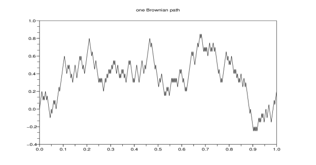
Figure 1: One path of the Brownian motion for $n=400$.

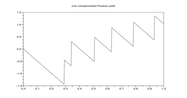
Figure 2: One path of the compensated Poisson process for $\lambda=5$ and $n=400$.

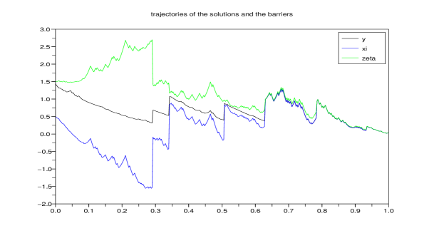
Figure 3: Trajectories of the solution ${y}^{n}$ and the barriers ${\xi}^{n}$ and ${\zeta}^{n}$ for $\lambda=5$ and $n=400$.

Appendix A Technical result for the implicit penalized scheme

In this Section, we use $N_{0}$ and $c$ introduced in Definition 4.2.

Lemma A.1.

Suppose Assumption 2.5 holds and $g$ is a Lipschitz driver. For each $p\in\mathbb{N}$ and $n\geq N_{0}$ we have

$$\sup_{j}\mathbb{E}[|y_{j}^{p,n}|^{2}]+\delta\sum_{j=0}^{n-1}\mathbb{E}[|z_{j}^{p,n}|^{2}]+\kappa_{n}(1-\kappa_{n})\sum_{j=0}^{n-1}\mathbb{E}[|u_{j}^{p,n}|^{2}]+\frac{1}{p\delta}\sum_{j=0}^{n-1}\mathbb{E}[|a_{j}^{p,n}|^{2}]+\frac{1}{p\delta}\sum_{j=0}^{n-1}\mathbb{E}[|k_{j}^{p,n}|^{2}]\leq c.$$

Proof.

By applying Lemma B.1 to the process $y^{p,n}$ between $i$ and $i+1$ and by suming the equality from $i=i$ to $i=n$, we get

$$\mathbb{E}[|y_{j}^{p,n}|^{2}]+\delta\sum_{i=j}^{n-1}\mathbb{E}[|z_{i}^{p,n}|^{2}] +\kappa_{n}(1-\kappa_{n})\sum_{i=j}^{n-1}\mathbb{E}[|u_{i}^{p,n}|^{2}]+\kappa_{n}(1-\kappa_{n})\sum_{i=j}^{n-1}\mathbb{E}[|v_{i}^{p,n}|^{2}]$$

$$\leq\mathbb{E}[|\xi^{n}_{n}|^{2}]+2\sum_{i=j}^{n-1}\mathbb{E}[|y_{i}^{p,n}||g(t_{i},y_{i}^{p,n},z_{i}^{p,n},u_{i}^{p,n})\delta|]+2\mathbb{E}[\sum_{i=j}^{n-1}(y_{i}^{p,n}a_{i}^{p,n}-y_{i}^{p,n}k_{i}^{p,n})].$$

Note that $y_{i}^{p,n}a_{i}^{p,n}=-\frac{1}{p\delta}(a_{i}^{p,n})^{2}+\xi_{i}^{n}a_{i}^{p,n}$ and $y_{i}^{p,n}k_{i}^{p,n}=\frac{1}{p\delta}(k_{i}^{p,n})^{2}+\zeta_{i}^{n}k_{i}^{p,n}$. We have that:

$$\mathbb{E}[|y_{j}^{p,n}|^{2}] +\frac{\delta}{2}\sum_{i=j}^{n-1}\mathbb{E}[|z_{i}^{p,n}|^{2}]+\frac{\kappa_{n}(1-\kappa_{n})}{2}\sum_{i=j}^{n-1}\mathbb{E}[|u_{i}^{p,n}|^{2}]+\frac{1}{p\delta}\sum_{i=j}^{n-1}\mathbb{E}[|a_{i}^{p,n}|^{2}]+\frac{1}{p\delta}\sum_{i=j}^{n-1}\mathbb{E}[|k_{i}^{p,n}|^{2}]$$

$$\leq\mathbb{E}[|\xi^{n}_{n}|^{2}]+\delta\mathbb{E}[\sum_{i=j}^{n-1}|g(t_{i},0,0,0)|^{2}]+2\delta\left(1+2C_{g}+2C_{g}^{2}+\frac{2C_{g}^{2}\delta}{\kappa_{n}(1-\kappa_{n})}\right)\sum_{i=j}^{n-1}\mathbb{E}[|y_{i}^{p,n}|^{2}]$$

$$+2\sum_{i=j}^{n-1}\mathbb{E}[(\xi_{i}^{n})a_{i}^{p,n}]-2\sum_{i=j}^{n-1}\mathbb{E}[(\zeta_{i}^{n})k_{i}^{p,n}].$$

We get $2\sum_{i=j}^{n-1}\mathbb{E}[(\xi_{i}^{n})a_{i}^{p,n}]\leq\alpha\mathbb{E}(\sup_{i}|\xi^{n}_{i}|^{2})+\frac{1}{\alpha}\mathbb{E}\left(\sum_{i=j}^{n-1}a_{i}^{p,n}\right)^{2}$ and $2\sum_{i=j}^{n-1}\mathbb{E}[(\zeta_{i}^{n})k_{i}^{p,n}]\leq\beta\mathbb{E}(\sup_{i}|\zeta^{n}_{i}|^{2})+\frac{1}{\beta}\mathbb{E}\left(\sum_{i=j}^{n-1}k_{i}^{p,n}\right)^{2}$. Following the same type of proof as [16, Lemma 2], we get

$$\mathbb{E}\left(\sum_{i=j}^{n-1}a_{i}^{p,n}\right)^{2}+\mathbb{E}\left(\sum_{i=j}^{n-1}k_{i}^{p,n}\right)^{2}\leq C(c+\mathbb{E}[\sum_{i=j}^{n-1}\delta(|y^{p,n}_{i}|^{2}+|z^{p,n}_{i}|^{2})+\kappa_{n}(1-\kappa_{n})(|u^{p,n}_{i}|^{2}+|v^{p,n}_{i}|^{2})].$$

Finally, by taking $\alpha=\beta=4C$ and by applying the Gronwall inequality (we recall $n\geq N_{0}$), we get that:

$$\sup_{j}\mathbb{E}[|y_{j}^{p,n}|^{2}+\frac{\delta}{4}\sum_{j=0}^{n-1}|z_{j}^{p,n}|^{2}+\frac{\kappa_{n}(1-\kappa_{n})}{4}\sum_{j=0}^{n-1}|u_{j}^{p,n}|^{2}+\frac{1}{p\delta}\sum_{j=0}^{n-1}|a_{j}^{p,n}|^{2}+\frac{1}{p\delta}\sum_{j=0}^{n-1}|k_{j}^{p,n}|^{2}]\leq c.$$

∎

Appendix B Some results on discrete stochastic calculus

In this section we present two lemmas which are used throughout the paper.

Lemma B.1.

Consider two integers $i_{0}$ and $i_{1}$ in ${0,...,N}$ and $(y_{n})_{n}$ a discrete process. We have

$$y_{i_{1}}^{2}=y_{i_{0}}^{2}+2y_{i_{0}}(y_{i_{1}}-y_{i_{0}})+(y_{i_{1}}-y_{i_{0}})^{2}.$$

The proof comes from the computation of $((b-a)+a)^{2}$, we omit it.

Lemma B.2.

(A discrete Gronwall lemma) Let $a$, $b$ and $\alpha$ be positive constants, $\delta b<1$ and a sequence $(v_{j})_{j=1,...n}$ of positive numbers such that for every $j$

$$v_{j}+\alpha\leq a+b\delta\sum_{i=1}^{j}v_{i}.$$

Then

$$\sup_{j\leq n}v_{j}+\alpha\leq ae^{bT}.$$

A proof of this lemma can be found in [17, Lemma 2.2], so we omit it.

References

- [1] B. Bouchard and R. Elie. Discrete-time approximation of decoupled Forward-Backward SDE with jumps. Stochastic Processes and their Applications, (118):53–75, 2008.
- [2] J.-F. Chassagneux. A discrete-time approximation for doubly reflected BSDEs. Adv. in Appl. Probab., 41(1):101–130, 2009.
- [3] S. Crépey and A. Matoussi. Reflected and doubly reflected BSDEs with jumps: a priori estimates and comparison. Ann. Appl. Probab., 18(5):2041–2069, 2008.
- [4] J. Cvitanic and I. Karatzas. Backward stochastic differential equations with reflection and Dynkin games. The Annals of Probability, (41):2024–2056, 1996.
- [5] R. Dumitrescu and C. Labart. Numerical approximation of doubly reflected BSDEs with jumps and RCLL obstacles. http://hal.archives-ouvertes.fr/hal-01006131, 2014.
- [6] R. Dumitrescu, M. Quenez, and A. Sulem. Double barrier reflected BSDEs with jumps and generalized Dynkin games. 2014.
- [7] N. El Karoui, C. Kapoudjian, E. Pardoux, S. Peng, and M. Quenez. Reflected solutions of Backward SDE’s and related obstacle problems for PDE’s. The Annals of Probability, 25(2):702–737, 1997.
- [8] E. Essaky. Reflected backward stochastic differential equation with jumps and RCLL obstacle. Bulletin des Sciences Mathématiques, (132):690–710, 2008.
- [9] E. Essaky, N. Harraj, and Y. Ouknine. Backward stochastic differential equation with two reflecting barriers and jumps. Stochastic Analysis and Applications, 23:921–938, 2005.
- [10] S. Hamadène and M. Hassani. BSDEs with two reacting barriers driven by a Brownian motion and an independent Poisson noise and related Dynkin game. Electronic Journal of Probability, 11:121–145, 2006.
- [11] S. Hamadène and Y. Ouknine. Reflected Backward Stochastic Differential Equation with jumps and random obstacle. Elec. Journ. of Prob., 8:1–20, 2003.
- [12] S. Hamadène and Y. Ouknine. Reflected Backward SDEs with general jumps. http://arxiv.org/abs/0812.3965, 2013.
- [13] S. Hamadène and H. Wang. BSDEs with two RCLL Reflecting Obstacles driven by a Brownian Motion and Poisson Measure and related Mixed Zero-Sum Games. Stochastic Processes and their Applications, 119:2881–2912, 2009.
- [14] J. Jacod and A. N. Shiryaev. Limit theorems for stochastic processes, volume 288 of Grundlehren der Mathematischen Wissenschaften [Fundamental Principles of Mathematical Sciences]. Springer-Verlag, Berlin, second edition, 2003.
- [15] A. Lejay, E. Mordecki, and S. Torres. Numerical approximation of Backward Stochastic Differential Equations with Jumps. https://hal.inria.fr/inria-00357992, Sept. 2014.
- [16] J. Lepeltier and J. San Martin. Backward SDEs with two barriers ans continuous coefficient: an existence result. Journal of Appl. Prob., (41):162–175, 2004.
- [17] J. Mémin, S. Peng, and M. Xu. Convergence of solutions of discrete Reflected backward SDE’s and Simulations. Acta Mathematica Sinica, 24(1):1–18, 2002.
- [18] E. Pardoux and S. Peng. Adapted solution of a backward stochastic differential equation. Systems Control Lett., 14(1):55–61, 1990.
- [19] S. Peng and M. Xu. Numerical algorithms for BSDEs with 1-d Brownian motion: convergence and simulation. ESAIM: Mathematical Modelling and Numerical Analysis, (45):335–360, 2011.
- [20] M. Quenez and A. Sulem. BSDEs with jumps, optimization and applications to dynamic risk measures. Stochastic Processes and their Applications, (123):3328–3357, 2013.
- [21] S. Tang and X. Li. Necessary conditions for optimal control of stochastic systems with random jumps. SIAM J. Cont. and Optim., 32:1447–1475, 1994.
- [22] M. Xu. Numerical algorithms and Simulations for Reflected Backward Stochastic Differential Equations with Two Continuous Barriers. Journal of Computational and Applied Mathematics, 236:1137–1154, 2011.