Brillouin precursors in Debye media

Abstract

We theoretically study the formation of Brillouin precursors in Debye media. We point out that the precursors are visible only at propagation distances such that the impulse response of the medium is essentially determined by the frequency dependence of its absorption and is practically Gaussian. By simple convolution, we then obtain explicit analytical expressions of the transmitted waves generated by reference incident waves, distinguishing precursor and main signal by a simple examination of the long-time behavior of the overall signal. These expressions are in good agreement with the signals obtained in numerical or real experiments performed on water in the radio-frequency domain and explain in particular some observed shapes of the precursor. Results are obtained for other remarkable incident waves. In addition, we show quite generally that the shape of the Brillouin precursor appearing alone at sufficiently large propagation distance and the law giving its amplitude as a function of this distance do not depend on the precise form of the incident wave but only on its integral properties. The incidence of a static conductivity of the medium is also examined and explicit analytical results are again given in the limit of weak and strong conductivities.

I INTRODUCTION

In their celebrated papers som14 ; bri14 ; bri32 ; bri60 on the propagation of a step-modulated optical wave through a single-resonance Lorentz medium, Sommerfeld and Brillouin found that, in suitable conditions, the arrival of the signal at the carrier frequency (“main signal”) is preceded by that of a first and a second transient, respectively generated from the high and low frequencies contained in the spectrum of the incident wave. More than a century after their discovery, these transients, currently named Sommerfeld and Brillouin precursors, continue to raise considerable interest, due in particular to their sub-exponential attenuation with the propagation distance. An abundant bibliography on the subject is given in Ref ou09 and more recent related studies are reported in Refs je09 ; ou10 ; bm11 ; cia11 ; bm12 .

In fact the simultaneous observation of well-distinguishable Sommerfeld and Brillouin precursors, as considered by their discoverers, requires experimental conditions that seem unrealizable in optics bm11 . A qualitative demonstration of separated Sommerfeld and Brillouin precursors has only been performed in microwaves by using guiding structures with dispersion characteristics similar to those of a Lorentz medium pl69 . In optics, only the unique precursor resulting from a complete overlapping of the Sommerfeld and Brillouin precursors aa88 ; bm13 has been actually observed bs87 ; aa91 ; je06 ; wei09 ; bm10 ; zh13 .

Precursors are obviously not specific to electromagnetic waves and Lorentz media. A convincing demonstration of Sommerfeld precursors has been performed by using elastic waves propagating on a liquid surface fa03 . We consider here electromagnetic waves propagating in dielectric media whose susceptibility is determined by the partial orientation of molecular dipoles under the effect of the applied electric field de30 . These currently called Debye media are opaque (transparent) at high (low) frequency. Only the Brillouin precursor is thus expected to be observable in good conditions, without the overlapping problem encountered in Lorentz media. Propagation of waves in Debye media has been extensively studied in the past, with particular attention paid to the important case of water in the radio-frequency and microwave domains. For papers related to the present study, see, e.g., Refs al89 ; ro96 ; fa97 ; ka98 ; li01 ; sto01 ; ro04 ; ou05 ; pi09 ; sa09 ; da10 ; ca11 ; bm12 ; ou12 . Albanese et al. were the first to refer to the Brillouin precursors in Debye media al89 . They numerically studied the propagation in water of sine waves at 1 GHz with square or trapezoidal envelopes and noticed “a well-formed transient field that appears similar to the Brillouin precursor observed in media with anomalous dispersion”. Stoudt et al. sto01 performed the corresponding experiments, achieving direct detection of Brillouin precursors. Indirect experimental demonstrations were achieved later pi09 ; da10 . Oughstun et al. theoretically studied at length the propagation of waves with a step, rectangular or trapezoidal envelope in Debye media by combining numerical computations and analytical calculations using saddle-point methods ou05 ; ou09 ; ou12 . Important features of the transmitted wave and, in particular, some remarkable shapes of the Brillouin precursor were unfortunately overlooked in these works.

In the present paper, the problem is greatly simplified by remarking that the precursor is only visible (discernible from the main signal) at propagation distances for which the impulse response of the medium is practically Gaussian. By convolution procedures, this enables us to obtain fully analytical expressions of the transmitted waves generated by different incident waves, distinguishing main signal and precursor by a simple examination of the long-time behavior of the overall signal. The arrangement of our paper is as follows. In Sec II, we present our approximation and give the corresponding impulse response of the medium. We derive in Sec III the transmitted wave generated from incident sine waves with a step or rectangular envelope. The response to sine-waves with linearly varying amplitude is studied in Sec IV. General properties of the precursors in the strict asymptotic limit are established in Sec V and the effects of a static conductivity of the medium are examined in Sec VI. We finally conclude in Sec VII by summarizing our main results.

II IMPULSE RESPONSE OF THE MEDIUM

As in the experiments on water reported in Refs fa97 ; sto01 , we consider transverse electromagnetic waves propagating in a coaxial transmission line containing the Debye medium. This coaxial geometry has the advantage of having a “flat frequency response down to and including DC” sto01 , as required for a good observation of the Brillouin precursors. We denote $\ell$ as the length of the transmission line, $v(0,t)$ [$v(\ell,t)$] as the voltage at its input [output] inside the medium and $V(0,\omega)$ [$V(\ell,\omega)$] as its Laplace-Fourier transform. In the frequency domain the medium is fully characterized by its transfer function $H(\ell,\omega)$ relating $V(\ell,\omega)$ to $V(0,\omega)$ pap87 :

.

$$V(\ell,\omega)=H(\ell,\omega)V(0,\omega)$$ (1)

with

$$H(\ell,\omega)=\exp\left[-i\frac{\omega\ell}{c}\tilde{n}(\omega)\right]$$ (2)

where $\omega$, $c$ and $\tilde{n}(\omega)$ are the (angular) frequency, the light velocity in vacuum and the complex refractive index of the medium, respectively. For Debye media, we have

$$\tilde{n}(\omega)=\sqrt{n_{\infty}^{2}+\frac{n_{0}^{2}-n_{\infty}^{2}}{1+i\omega\tau}}$$ (3)

In this expression $n_{\infty}$, $n_{0}$ and $\tau$ respectively denote the refractive index at high frequency (Debye plateau), the refractive index at vanishing frequency and the orientation relaxation time of the polar molecules. Eq.(3) provides a good approximation of the refractive index of Debye media in the radiofrequency and microwave domains. For deionized water, often taken as reference, $n_{0}^{2}\approx 79$ , $n_{\infty}^{2}\approx 5.5$ and $\tau\approx 8.5\,\mathrm{ps}$ may be considered as typical values sto01 and are used in our calculations. For the frequencies up to 100 GHz the real and imaginary parts of the refractive index derived from Eq. (3) with these parameters fit very well the measurements reported in Ref se81 .

In the time domain, the medium will be characterized by its impulse response $h(\ell,t)$, which is the inverse Fourier transform of $H(\ell,\omega)$, and the output voltage is given by the convolution product

$$v(\ell,t)=h(\ell,t)\otimes v(0,t)$$ (4)

$h(\ell,t)$ has no exact analytical form. Some general properties of $h(\ell,t)$ can however be derived from $H(\ell,\omega)$. The relation $\intop_{-\infty}^{+\infty}h(\ell,t)\,dt=H(\ell,0)=1$ shows that it has a unit area. The location of its center of gravity $t_{B}=\left(\intop_{-\infty}^{+\infty}t\,h(\ell,t)\,dt\right)/\left(\intop_{-\infty}^{+\infty}h(\ell,t)\,dt\right)$, its centered second moment or variance $\sigma^{2}=\left(\intop_{-\infty}^{+\infty}(t-t_{B})^{2}\,h(\ell,t)\,dt\right)/\left(\intop_{-\infty}^{+\infty}h(\ell,t)\,dt\right)$ and its centered third moment $\mu_{3}=\left(\intop_{-\infty}^{+\infty}(t-t_{B})^{3}\,h(\ell,t)\,dt\right)/\left(\intop_{-\infty}^{+\infty}h(\ell,t)\,dt\right)$ are respectively equal to the cumulants $k_{1}$, $k_{2}$ and $k_{3}$ of the transfer function bu04 as defined in the following expansion:

$$H(\ell,\omega)=\exp\left(\sum_{n=1}^{\infty}\frac{\left(-i\omega\right)^{n}}{n!}k_{n}\left(\ell\right)\right)$$ (5)

In the case of a Debye medium, we deduce from Eqs.(2) and (3) $t_{B}=n_{0}\ell/c$ , $\sigma^{2}=\frac{n_{0}^{2}-n_{\infty}^{2}}{n_{0}}\left(\frac{\ell\tau}{c}\right)$ and $\mu_{3}=\frac{3\left(n_{0}^{2}-n_{\infty}^{2}\right)\left(3n_{0}^{2}+n_{\infty}^{2}\right)}{4n_{0}^{3}}\left(\frac{\ell\tau^{2}}{c}\right)$. These expressions show that the center of gravity of $h(\ell,t)$ propagates at the phase velocity at zero frequency (equal to the group velocity for this frequency) and has a root-mean-square duration $\sigma$ proportional to $\sqrt{\ell}$ and a positive skewness or asymmetry $\xi=\tfrac{\mu_{3}}{\sigma^{3}}=\frac{3\left(3n_{0}^{2}+n_{\infty}^{2}\right)}{4\sqrt{n_{0}^{3}\left(n_{0}^{2}-n_{\infty}^{2}\right)}}\sqrt{\frac{c\tau}{\ell}}$.

The previous results are valid for arbitrary propagation distances. The expression of the skewness ($\xi\varpropto 1/\sqrt{\ell}$) suggests that the expansion of Eq. (5) may be limited to the term $n=2$ when $\ell$ is large enough. Taking the origin of time at $t=t_{B}$, the transfer function and the impulse response are reduced to the Gaussians

$$H(\ell,\omega)=e^{-\omega^{2}/(4\beta^{2})}=e^{-\alpha(\omega)\ell}$$ (6)

$$h(\ell,t)=\frac{\beta}{\sqrt{\pi}}e^{-\beta^{2}t^{2}}$$ (7)

where $\alpha(\omega)$ is the absorption coefficient of the medium at the frequency $\omega$ and

$$\beta=\frac{1}{\sigma\sqrt{2}}=\sqrt{\frac{cn_{0}}{2\ell\tau\left(n_{0}^{2}-n_{\infty}^{2}\right)}}$$ (8)

$h(\ell,t)$ has then a peak amplitude (a duration) proportional to $1/\sqrt{\ell}$ ($\sqrt{\ell}$) with a unit area, as expected. It meets the principle of relativistic causality re0 as long as $\exp\left[-\beta^{2}\left(n_{0}-n_{\infty}\right)^{2}\left(\ell/c\right)^{2}\right]$ is negligible, a condition superabundantly satisfied for the propagation distances at which the Brillouin precursor is visible. Decomposing the medium in $m$ subsections of impulse response $h(\ell/m,t)$, the Gaussian form of $h(\ell,t)$ given by Eq. (7) may be considered as a consequence of the central limit theorem in a deterministic case pap87 . It is also the limit when $\beta t_{B}\gg 1$ of the expressions of $h(\ell,t)$ obtained by direct studies in the time-domain ro96 ; ka98 ; ro04 . When $\xi\ll 1$, the condition $\beta t_{B}\gg 1$ is automatically fulfilled and the Gaussian form $h(\ell,t)$ given by Eq. (7) is expected to hold. This is illustrated Fig 1, obtained for $\ell=10\,\mathrm{cm}$ in deionized water.

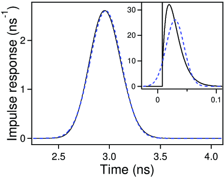
Figure 1: (Color online) Impulse response of deionized water as a function of time for a propagation distance $\ell=10\>\mathrm{cm}$ leading to $t_{B}=2.96\>\mathrm{ns}$ and $\beta=4.63\>\mathrm{\mathrm{n}s^{-1}}$. The solid [dashed] line is the exact numerical result obtained by FFT [the Gaussian shape given by Eq. (7)]. Inset: the same for $\ell=1\>\mathrm{mm}$, leading to $t_{B}=29.6\>\mathrm{ps}$ and $\beta=46.3\>\mathrm{\mathrm{n}s^{-1}}$.

We have then $\beta t_{B}\approx 13.7$ and the result given by Eq. (7) is actually very close to the exact result, numerically derived from the exact transfer function by fast Fourier transform (FFT). The main effect of the residual skewness is a very slight reduction of the time of the maximum by about $9.5\,\mathrm{ps}$ whereas $t_{B}\approx 2.96\,\mathrm{ns}$. For $\ell=1\>\mathrm{cm}$ ($\beta t_{B}\approx 4.3$), the skewness increases and the rise of $h(\ell,t)$ becomes significantly steeper than its fall. However the Gaussian form of Eq. (7) remains a reasonable approximation of the exact result. This approximation completely fails when $\beta t_{B}\lesssim 1$ . The impulse response then begins at the time $n_{\infty}\ell/c$ re0 by a Dirac peak and a discontinuity. The weight $w$ of the former and the amplitude $\Delta h$ of the latter are easily determined from an asymptotic expansion of $H(\ell,\omega)$. We get $w=\exp\left[-\left(n_{0}^{2}-n_{\infty}^{2}\right)\ell/\left(2n_{\infty}c\tau\right)\right]$ and $\Delta h=w\ell\left(n_{0}^{2}-n_{\infty}^{2}\right)\left(n_{0}^{2}+3n_{\infty}^{2}\right)/\left(8c\tau^{2}n_{\infty}^{3}\right)$. The inset of Fig. 1 shows the impulse response obtained for $\ell=1\>\mathrm{mm}$ ($\beta t_{B}\approx 1.37$). We have then $w\approx 2.14\times 10^{-3}$ and $\Delta h\approx 6.7\,\mathrm{ns^{-1}}$. The previous results are only given for completeness. Indeed, it will be shown later that the Brillouin precursor emerges from the main signal for $\ell>20\>\mathrm{cm}$ ($\beta t_{B}>19.4$ ) and the Gaussian approximation of $h(\ell,t)$ is then excellent. Note that this remarkable form of the impulse response is not specific to the Debye medium but holds at large enough propagation distances whenever the transfer function can be expanded in cumulants. It applies in particular to polar media with relaxation mechanisms more complex than those considered here. We incidentally note that the addition of a second relaxation time in the Debye model as considered in Refs ou05 ; ou09 does not significantly modify the parameters $t_{B}$ and $\beta$.

The considerable advantage of the Gaussian impulse response is that it can be convoluted with a great number of input signals to provide exact analytical forms of the output signal. This is the case, e.g., when $v(0,t)$ is a step, an algebraic function, an exponential, a Gaussian or an error function, when these functions modulate a sine wave (eventually linearly chirped) or when $v(0,t)$ is a combination of the previous signals al89 ; li01 ; sto01 ; ou05 ; ou09 ; da10 ; ou12 ; bm12 . The relation $V(\ell,0)=H(\ell,0)V(0,0)$ quite generally shows that the area of the output signal will be always equal to that of the input signal. We also remark that the Gaussian impulse response is obtained by neglecting the effects of the group-velocity dispersion. This explains why the shape of the output signals observed in the experiments reported in Ref sto01 was well reproduced by numerical simulations taking only into account the frequency-dependence of the medium absorption. This also means that the Brillouin precursors actually observed or observable in Debye media essentially originate from the latter and that group-velocity dispersion plays no significant role in their formation.

In the previous theoretical analysis it is assumed as usual that the input and output signals are measured inside the Debye medium. This is generally not the case in the experiments. $H(\ell,\omega)$ should then be multiplied by the transfer function $T(\omega)$ taking into account the losses at the air-medium and medium-air interfaces, that is

$$T(\omega)=\left[\frac{2}{1+\widetilde{n}(\omega)}\right]\times\left[\frac{2}{1+1/\widetilde{n}(\omega)}\right]=\frac{4\widetilde{n}(\omega)}{\left[1+\widetilde{n}(\omega)\right]^{2}}$$ (9)

The main effect of $T(\omega)$ will be an overall reduction of the amplitude of the output voltage by a factor $1/T(0)=\left(n_{0}+1\right)^{2}/\left(4n_{0}\right)$ that is $2.75$ for deionized water. The frequency-dependent effects can be determined by expanding $T(\omega)/T(0)$ in cumulants as made for $H(\ell,\omega)$ and exploiting the additivity property of the cumulants. Again for deionized water, we find that $t_{B}$ ($\sigma^{2}$) is reduced by about $3.15\,\mathrm{ps}$ ($15.7\,\mathrm{ps^{2}}$). For $\ell\geq 10\,\mathrm{cm}$, these quantities are fully negligible compared to those associated with $H(\ell,\omega)$. The output signals determined from $H(\ell,\omega)$ in the following should thus be simply multiplied by $T(0)=4n_{0}/\left(1+n_{0}\right)^{2}$ and delayed by the extra transit times in air when the voltages are measured outside the medium.

III RESPONSE TO STEP-MODULATED SINE-WAVES

We consider in this section input signals of the form $u_{H}(t)\sin\left(\omega_{c}t\right)$ or $u_{H}(t)\cos\left(\omega_{c}t\right)$, where $u_{H}(t)$ is the Heaviside unit step function. They consist of a sine wave of angular frequency $\omega_{c}$ (the “carrier”) switched on at time $t=0$. The former is the “canonical” signal used by Sommerfeld and Brillouin. Both cases can be jointly studied by considering the complex input signal $\tilde{v}(0,t)=u_{H}(t)\exp\left(i\omega_{c}t\right)$. Its convolution with the Gaussian impulse response gives for the corresponding output signal

$$\tilde{v}(\ell,t)\thickapprox\frac{1}{2}\left[1+\mathrm{erf}\left(\beta t+iy\right)\right]e^{-y^{2}}e^{i\omega_{c}t}$$ (10)

Here $\mathrm{erf}(z)$ indicates the error function, $t$ is the time retarded by $t_{B}$, and $y=\omega_{c}/\left(2\beta\right)=\sqrt{\alpha_{c}\ell}$, where $\alpha_{c}$ is a short-hand notation for $\alpha\left(\omega_{c}\right)$. Taking $t_{B}$ ($1/\beta$) as time origin (time scale), Eq.(10) shows that the output signal only depends on $y$. For sufficiently large $t$, this signal becomes

$$\tilde{v}_{m}(\ell,t)\thickapprox\frac{1}{2}\left[1+\mathrm{erf}\left(\beta t\right)\right]e^{-\alpha_{c}\ell}e^{i\omega_{c}t}$$ (11)

and tends to $\tilde{v}_{m}(\ell,t)\thickapprox e^{-\alpha_{c}\ell}e^{i\omega_{c}t}$ when $t\rightarrow\infty$. This part of $\tilde{v}(\ell,t)$ given by Eq.(11) may naturally be identified to the main signal. The Brillouin precursor is then given by the remaining part, that is

$$\tilde{v}_{p}(\ell,t)\thickapprox\frac{1}{2}\left[\mathrm{erf}\left(\beta t+i\sqrt{\alpha_{c}\ell}\right)\mathrm{-erf}\left(\beta t\right)\right]e^{-\alpha_{c}\ell}e^{i\omega_{c}t}$$ (12)

Since $\omega_{c}=2\beta\sqrt{\alpha_{c}\ell}$, all the previous signals appear as universal functions of $\beta t$ or of $\omega_{c}t$ that only depend on the optical thickness $\alpha_{c}\ell$ of the medium at the frequency $\omega_{c}$ of the carrier. To be definite we consider in the following deionized water and a carrier frequency $\omega_{c}=2\pi\times 10^{9}\,\mathrm{s^{-1}}$, i.e., a period $T_{c}=1\,\mathrm{ns}$ as often considered in the literature al89 ; sto01 ; ou05 ; ou09 . We, however, emphasize that our analytical results are quite general.

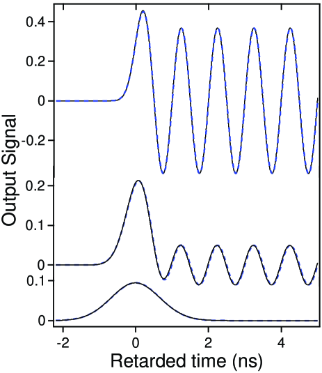
Figure 2: (Color online) Responses to the input signal $u_{H}(t)\sin(\omega_{c}t)$ as a function of the time retarded by $t_{B}$, for $\alpha_{c}\ell=1,\,3\>\mathrm{and}\>10$ (from top to bottom). The solid (dashed) lines give the exact numerical solution (our analytical solution in terms of error functions). Note that for the carrier frequency considered ($\omega_{c}/(2\pi)=1\>\mathrm{\mathrm{n}s^{-1}}$), the optical thickness $\alpha_{c}\ell=1$ is attained for $\ell=21.6\>\mathrm{cm}$.

The responses to the canonical input signal $u_{H}(t)\sin\left(\omega_{c}t\right)$ are obtained by taking the imaginary part of Eqs. (10à)-(12). Figure 2 shows the output signals $v(\ell,t)$ obtained for different values of $\alpha_{c}\ell$. As expected, they reproduce very well the exact signals obtained by a FFT calculation of the inverse Fourier transform of $H(\ell,\omega)V(0,\omega)$. For $\alpha_{c}\ell=1$ ($\ell\approx 21.6\,\mathrm{cm}$), the precursor appears as a small overshot on $v(\ell,t)$, which is hardly visible for smaller optical thicknesses. For $\alpha_{c}\ell=3$, we have an example of well developed precursor dominating the main signal. Finally for $\alpha_{c}\ell=10$, the main signal is extremely small and only the precursor remains visible. Figure 3 shows the corresponding precursors alone, as defined by Eq. (12). Owing to the symmetry properties of the real and imaginary parts of the error function, they are even functions of $t$. Their peak amplitude is simply

$$A_{p}(\ell)=\mathrm{Im}\left[\tilde{v}_{p}(\ell,0)\right]=\frac{\mathrm{erf}\left(i\sqrt{\alpha_{c}\ell}\right)}{2i}e^{-\alpha_{c}\ell},$$ (13)

whereas their area $S_{p}\left(\ell\right)$ , also deduced from Eq. (12), reads as

$$S_{p}\left(\ell\right)=\frac{\left(1-e^{-2\alpha_{c}\ell}\right)}{\omega_{c}}.$$ (14)

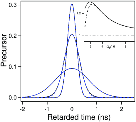
Figure 3: (Color online) Analytical forms of the precursor contribution to the signals of Fig. 2 (solid lines) and their approximation by the Gaussian given in Eq. (15) (dashed lines). Inset : ratios of $\beta_{p}$ (solid line) and $A_{p}$ (dashed line) over their asymptotic values as a function of the optical thickness.

Remarkably enough, their shape is practically Gaussian. The precursor part of the output signal can thus be written under the approximate form

$$v_{p}\left(\ell,t\right)=A_{p}(\ell)\,e^{-\beta_{p}^{2}t^{2}},$$ (15)

where the parameter $\beta_{p}$ is easily determined by combining Eqs. (13) and (14). We get

$$\beta_{p}=\frac{\sqrt{\pi\alpha_{c}\ell}\mathrm{\,erf}\left(i\sqrt{\alpha_{c}\ell}\right)}{i\left(e^{\alpha_{c}\ell}-e^{-\alpha_{c}\ell}\right)}\beta.$$ (16)

As shown in Fig. 3, Eq. (15), with $A_{p}$ and $\beta_{p}$ given by Eq. (13) and (16), provides an excellent approximation of the exact result. It strictly gives the exact result when $\alpha_{c}\ell\rightarrow\infty$. From the asymptotic form of the error function ni10 , we then get $A_{p}(\ell)=\frac{1}{2\sqrt{\pi\alpha_{c}\ell}}=\frac{\beta}{\omega_{c}\sqrt{\pi}}$ and $\beta_{p}=\beta$, that is,

$$v_{p}\left(\ell,t\right)=\frac{\beta}{\omega_{c}\sqrt{\pi}}e^{-\beta^{2}t^{2}}=\frac{e^{-\beta^{2}t^{2}}}{2\sqrt{\pi\alpha_{c}\ell}}.$$ (17)

The well-known law $A_{p}(\ell)\propto 1/\sqrt{\ell}$ is retrieved but we remark that it only holds for very large optical thicknesses. When $\alpha_{c}\ell$ is only large (such that $e^{-\alpha_{c}\ell}\ll 1$), it is possible to obtain a better approximation of $v_{p}\left(\ell,t\right)$ by considering one more term in the asymptotic expansion of the error function ni10 . This leads to a simple multiplication of $\beta$ by $\sqrt{1+1/\left(\alpha_{c}\ell\right)}$ in the first form of Eq. (17). The inset of Fig. 3 more generally shows how the ratios of $\beta_{p}$ and $A_{p}$ over their asymptotic limit (respectively $\beta$ and $\frac{\beta}{\omega_{c}\sqrt{\pi}}$) vary as a function of $\alpha_{c}\ell$.

We examine briefly the case where $v(0,t)=u_{H}(t)\cos\left(\omega_{c}t\right)$. Such an input field originates a class of precursors whose amplitude depends on $\ell$ according to a law differing from the previous one. We incidentally remark that, for $\omega_{c}=0$ (no carrier), the output signal is nothing other than the step response of the medium pap87 that reads as $a(\ell,t)=\left[1+erf\left(\beta t\right)\right]/2$, a result in agreement with the observations reported in Refs fa97 ; sto01 . For $\omega_{c}\neq 0$ , the output signals are obtained by taking the real parts of Eqs. (10)-(12).

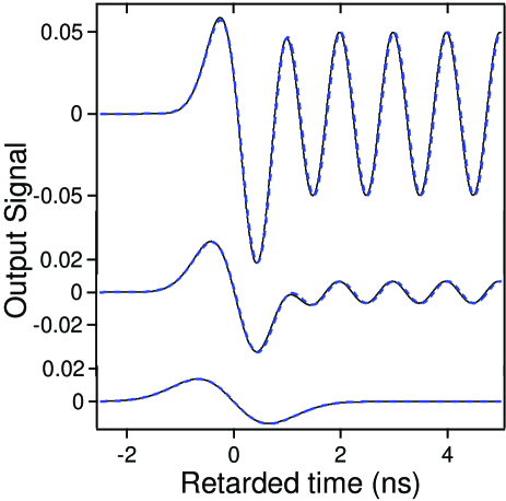
Figure 4: (Color online) Same as Fig. 2 when $v(0,t)=u_{H}(t)\cos(\omega_{c}t)$ for $\alpha_{c}\ell=3,\,5,\>\mathrm{and}\>10$ (from top to bottom).

Figure 4 shows the output signals $v(\ell,t)$ obtained for $\alpha_{c}\ell=3$, $5$, and $10$. The precursor appears for propagation distances larger than in the previous case and is not discernible from the main signal when $\alpha_{c}\ell=1$. The output signals $v(\ell,t)$ derived from Eq. (10) again fit very well the exact signals obtained by FFT. The contribution $v_{p}(\ell,t)$ of the precursor to the output signal (Fig. 5) is now an odd function of $t$. Its slope at $t=0$ can be determined by expanding Eq. (12) at the first order in $t$. We get $\dot{v}_{p}\left(\ell,0\right)=-B_{p}$, with

$$B_{p}=\beta\left[\sqrt{\alpha_{c}\ell}\frac{\mathrm{erf}\left(i\sqrt{\alpha_{c}\ell}\right)}{i}e^{-\alpha_{c}\ell}-\frac{1-e^{-\alpha_{c}\ell}}{\sqrt{\pi}}\right]>0.$$ (18)

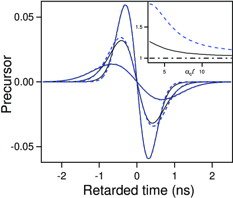
Figure 5: (Color online) Analytical forms of the precursor contribution to the signals of Fig. 4 (solid lines) and their approximation by the Gaussian derivative given Eq. (19) (dashed lines). Inset is the same that of Fig. 3.

The precursors are now well fitted by derivatives of Gaussian (Fig. 5) and can be written as $v_{p}(\ell,t)\thickapprox-B_{p}te^{-\gamma_{p}^{2}t^{2}}$. In fact, $\gamma_{p}$, achieving the best fit, never considerably differs from $\beta_{p}$. The precursor takes then the approximate form

$$v_{p}(\ell,t)\approx-B_{p}te^{-\beta_{p}^{2}t^{2}}=\frac{B_{p}}{2\beta_{p}^{2}}\frac{d}{dt}e^{-\beta_{p}^{2}t^{2}}$$ (19)

with a peak amplitude

$$A_{p}(\ell)=\frac{B_{p}}{\beta_{p}\sqrt{2e}}.$$ (20)

As shown in Fig. 5, Eq. (19) provides a satisfactory approximation of the precursor. It gives the exact result when $\alpha_{c}\ell\rightarrow\infty$. In this limit, $\beta_{p}=\beta$, $B_{p}=2\beta^{3}/\left(\omega_{c}^{2}\sqrt{\pi}\right)$, $A_{p}(\ell)=1/\left(2\alpha_{c}\ell\sqrt{2e\pi}\right)$ and

$$v_{p}(\ell,t)=\left(\frac{\beta}{\omega_{c}^{2}\sqrt{\pi}}\right)\frac{d}{dt}\left(e^{-\beta^{2}t^{2}}\right)=\\ -\left(\frac{1}{2\alpha_{c}\ell\sqrt{\pi}}\right)\beta t\,e^{-\beta^{2}t^{2}}.$$ (21)

Since $\omega_{c}u_{H}(t)\cos\left(\omega_{c}t\right)=\frac{d}{dt}\left[u_{H}(t)\sin\left(\omega_{c}t\right)\right]$ and $v_{p}(\ell,t)=v(\ell,t)$ when $\alpha_{c}\ell\rightarrow\infty$, this precursor is the time derivative of that obtained in the canonical case [see Eq.(17)] divided by $\omega_{c}$. Its amplitude now scales as $1/\ell$ instead as $1/\sqrt{\ell}$ in the previous case. As shown in the inset of Fig. 5, this law only holds for very large optical thicknesses.

From the results obtained with the input signals $u_{H}(t)\sin\left(\omega_{c}t\right)$ and $u_{H}(t)\cos\left(\omega_{c}t\right)$, the responses to the more general input signal $u_{H}(t)\sin\left(\omega_{c}t+\varphi\right)$ are easily determined. The precursor is then a superposition of a Gaussian and a Gaussian derivative with relative amplitudes depending on $\varphi$ and on the propagation distance.

In real or numerical experiments, the input signal has obviously a finite duration. One generally considers input signals with a rectangular envelope of duration $T$ long enough to avoid having the precursors generated by the rise and the fall of the pulse overlap. The corresponding complex signal reads as $\tilde{v}_{R}(0,t)=\left[u_{H}(t)-u_{H}(t-T)\right]e^{i\omega_{c}t}$, that is

$$\tilde{v}_{R}(0,t)=u_{H}(t)\,e^{i\omega_{c}t}-e^{i\omega_{c}T}u_{H}(t-T)\,e^{i\omega_{c}\left(t-T\right)}.$$ (22)

It generates the output signal

$$\tilde{v}_{R}(\ell,t)=\tilde{v}(\ell,t)-e^{i\omega_{c}T}\,\tilde{v}(\ell,t-T),$$ (23)

where $\tilde{v}(\ell,t)$ is given by Eq. (10). No matter $T$, the mains signals generated by the rise and the fall of the pulse destructively interferes when $\beta\left(t-T\right)\gg\sqrt{\alpha_{c}\ell}$. On the other hand, the second precursor (a postcursor since it follows the main signal) generally differs from the first one owing to the phase factor $e^{i\omega_{c}T}$. Precursor and postcursor are identical only when $T=\left(2n+1\right)T_{c}/2$, where $n$ is an integer. They have the same shape and amplitude but opposite signs when $T=nT_{c}$. Both cases have been evidenced in the experiments reported in Ref sto01 . The largest difference between precursor and postcursor is attained when $T=\left(2n+1\right)T_{c}/4$. In this case $e^{i\omega_{c}T}=\left(-1\right)^{n}i$. For an input signal $v(0,t)=\left[u_{H}(t)-u_{H}(t-T)\right]\,\sin\left(\omega_{c}t\right)$, we get an output signal

$$v_{R}(\ell,t)=\mathrm{Im}\left[\tilde{v}(\ell,t)\right]-\left(-1\right)^{n}\mathrm{Re}\left[\tilde{v}(\ell,t-T)\right]$$ (24)

The precursor is then Gaussian [see Eq. (15)] whereas the postcursor is a Gaussian derivative [see Eq. (19)] of smaller amplitude. The opposite occurs for an input signal $v(0,t)=\left[u_{H}(t)-u_{H}(t-T)\right]\,\cos\left(\omega_{c}t\right)$. These various behaviors are illustrated in Fig. 6.

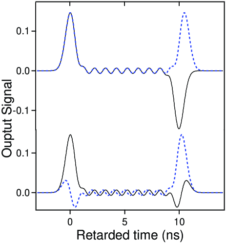
Figure 6: (Color online) Responses to input signals with a long rectangular envelope for $\alpha_{c}\ell=5$. The upper curves are obtained for $v(0,t)\propto\sin(\omega_{c}t)$ with $T=10\,T_{c}$ (solid line) and $T=10.5\,T_{c}$ (dashed line). The lower curves are obtained for $T=10.25\,T_{c}$ with $v(0,t)\propto\sin(\omega_{c}t)$ (solid line) and $v(0,t)\propto\cos(\omega_{c}t)$ (dotted line). Note that, in the latter case, the postcursor can completely dominate the precursor.

Equation (23) remains valid when the two precursors overlap and interfere to give a unique transient that may be considered as a generalized precursor. A remarkable behavior is obtained for an input signal $\left[u_{H}(t)-u_{H}(t-T_{c})\right]\,\cos\left(\omega_{c}t\right)$. A good overlapping of the precursors is achieved when $1/\beta\gg T_{c}$, that is in the asymptotic limit. We then get

$$v(\ell,t)\thickapprox v_{p}(\ell,t)-v_{p}(\ell,t-T_{c})\approx T_{c}\dot{v}_{p}\left(\ell,t-\frac{T_{c}}{2}\right),$$ (25)

where $v_{p}(\ell,t)$ is given by Eq. (21), and finally

$$v(\ell,\theta)=\left(\frac{2\beta\sqrt{\pi}}{\omega_{c}^{3}}\right)\frac{d^{2}}{d\theta^{2}}\left(e^{-\beta^{2}\theta^{2}}\right)=\\ -A_{\infty}\left(1-2\beta^{2}\theta^{2)}\right)e^{-\beta^{2}\theta^{2}},$$ (26)

where $\theta=t-T_{c}/2$ and $A_{\infty}=\left(\sqrt{\pi}/2\right)\left(\alpha_{c}\ell\right)^{-3/2}$. The output signal has now the shape of a Gaussian second-derivative centered at $t=T_{c}/2$ and a peak amplitude $A_{\infty}$ scaling as $\ell^{-3/2}$. For any optical thickness, it is easily shown from Eq.(23) that $v(\ell,\theta)$ is an even function of $\theta$ with a minimum at $\theta=0$ of algebraic amplitude $-A$, with

$$A=e^{-\alpha_{c}\ell}\,\mathrm{Re}\left[\mathrm{erf}\left(\frac{\pi\beta}{\omega_{c}}+i\frac{\omega_{c}}{2\beta}\right)\right]$$ (27)

that tends to $A_{\infty}$ when $\alpha_{c}\ell\rightarrow\infty$. It also results from Eq. (23) that

$$v\left(\ell,\theta\right)=\frac{e^{-\alpha_{c}\ell}}{2}\,\mathrm{Re}\left[\mathrm{erf}\left(\frac{2\pi\beta}{\omega_{c}}+i\frac{\omega_{c}}{2\beta}\right)\right]$$ (28)

for $\theta=\pm\pi/\omega_{c}$, that is, at the switching times of the input signal delayed by $t_{B}$. Unexpectedly enough, extensive numerical simulations show that $v\left(\ell,\theta\right)$ is very well fitted by a Gaussian second derivative as soon as $\alpha_{c}\ell>1$. The output signal then reads as

$$v\left(\ell,\theta\right)=-A\left(1-2\eta^{2}\beta^{2}\theta^{2}\right)e^{-\eta^{2}\beta^{2}\mathit{\theta}^{2}},$$ (29)

where $A$ is given by Eqs. (27) and $\eta$ is a parameter obtained by combing Eq. (27) and (28). Figure 7 shows the result obtained by this method for $\alpha_{c}\ell=5$. It perfectly fits the exact numerical result obtained by FFT. The asymptotic result of Eq. (26) is also given for comparison. In spite of the moderate value of the optical thickness, it is reasonable approximation of the exact result.

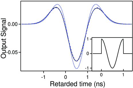
Figure 7: (Color online) Response to the input signal $\left[u_{H}(t)-u_{H}(t-T_{c})\right]\cos(\omega_{c}t)$ for $\alpha_{c}\ell=5$. The solid, dashed and dotted lines are the exact FFT solution, the approximate analytical solution given Eq. (29), and the asymptotic solution given Eq. (26), respectively. Inset: input signal.

IV RESPONSE TO SINE-WAVES WITH LINEARLY VARYING AMPLITUDE

We consider in this section input signals of the form $\left(t/T_{r}\right)u_{H}(t)\sin\left(\omega_{c}t\right)$ or $\left(t/T_{r}\right)u_{H}(t)\cos\left(\omega_{c}t\right)$ where $T_{r}$ is the time for which their amplitude equals 1 (rise time). Such signals can generate precursors preceding significantly the rise of the main signal. The corresponding complex signal reads as $\tilde{v}(0,t)=\left(t/T_{r}\right)u_{H}(t)\,e^{i\omega_{c}t}$. By convoluting this signal with the Gaussian impulse response, we get

$$\tilde{v}(\ell,t)=\frac{e^{-\beta^{2}t^{2}}}{2\beta T_{r}\sqrt{\pi}}+\frac{e^{-\alpha_{c}\ell}}{2\beta T_{r}}\times\\ \left\{\left(\beta t+i\sqrt{\alpha_{c}\ell}\right)\left[1+\mathrm{erf}\left(\beta t+i\sqrt{\alpha_{c}\ell}\right)\right]\right\}e^{i\omega_{c}t}.$$ (30)

Proceeding as in the previous section, we get for the main signal and the precursor

$$\tilde{v}_{m}(\ell,t)=\frac{e^{-\alpha_{c}\ell}}{2\beta T_{r}}\left\{\left(\beta t+i\sqrt{\alpha_{c}\ell}\right)\left[1+\mathrm{erf}\left(\beta t\right)\right]\right\}e^{i\omega_{c}t},$$ (31)

$$\tilde{v}_{p}(\ell,t)=\tilde{v}(\ell,t)-\tilde{v}_{m}(\ell,t).$$ (32)

All these signals are inversely proportional to $T_{r}$, and $\omega_{c}$ being fixed, it is convenient to normalize them to $1/\left(\omega_{c}T_{r}\right)$.

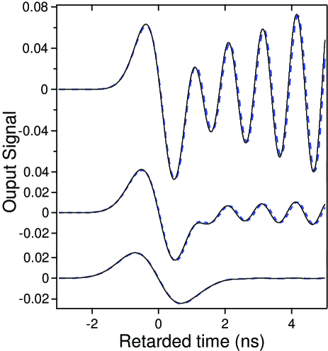
Figure 8: (Color online) Responses to the input signal $(t/T_{r})u_{H}(t)\sin(\omega_{c}t)$ normalized to $1/(\omega_{c}T_{r})$ for $\alpha_{c}\ell=6$, $8$, and $12$ (from top to bottom). The solid (dashed) line is the FFT exact solution (the approximate analytical solution in terms of error functions).

Figure 8 shows the output signal $v(\ell,t)=\mathrm{Im}\left[\tilde{v}(\ell,t)\right]$ generated by $v(0,t)=\left(t/T_{r}\right)u_{H}(t)\sin\left(\omega_{c}t\right)$ for different optical thicknesses. The precursor becomes discernible from the main field for $\alpha_{c}\ell\geq 6$ and is fully separated from it for $\alpha_{c}\ell=12$. In every case the analytical result derived from Eq. (30) fits very well the exact numerical result obtained by FFT. The contribution $v_{p}(\ell,t)=\mathrm{Im}\left[\tilde{v_{p}}(\ell,t)\right]$ of the precursor to the output signal is now an odd function of the retarded time $t$ and, for $\alpha_{c}\ell\geq 6$ , is well fitted by a Gaussian derivative (Fig. 9). This result is rigorous when $\alpha_{c}\ell\rightarrow\infty$ . By means of asymptotic expansions of the error function limited to its first non zero term in $1/\sqrt{\alpha_{c}\ell}$, we then get

$$v_{p}(\ell,t)=-\left(\frac{1}{\omega_{c}T_{r}}\right)\left(\frac{1}{\alpha_{c}\ell\sqrt{\pi}}\right)\beta t\,e^{-\beta^{2}t^{2}}=\\ \left(\frac{2\beta}{\omega_{c}^{3}T_{r}\sqrt{\pi}}\right)\frac{d}{dt}\left(e^{-\beta^{2}t^{2}}\right),$$ (33)

the precursor amplitude scaling as $1/\ell$.

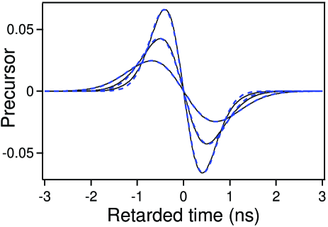
Figure 9: (Color online) Analytical forms of the precursor contribution to the signals of Fig. 8 (solid lines) and their best fit by Gaussian derivatives (dashed lines).

When $v(0,t)=\left(t/T_{r}\right)u_{H}(t)\cos\left(\omega_{c}t\right)$ , the overall output signal and the precursor read as $v(\ell,t)=\mathrm{Re}\left[\tilde{v}(\ell,t)\right]$ and $v_{p}(\ell,t)=\mathrm{Re}\left[\tilde{v_{p}}(\ell,t)\right]$ . The precursor becomes discernible from the main field for $\alpha_{c}\ell\geq 4.5$ (Fig. 10) and, again owing to the symmetry properties of the error function, is an even function of $t$.

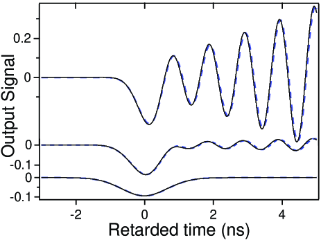
Figure 10: (Color online) Same as Fig. 8 with $v(0,t)=(t/T_{r})u_{H}(t)\cos(\omega_{c}t)$ for $\alpha_{c}\ell=4.5$, $7$, and $12$ (from top to bottom).

At $t=0$, $v_{p}(\ell,t)$ has the remarkable value

$$v_{p}(\ell,0)=-A=\frac{1}{\omega_{c}T_{r}}\left[\sqrt{\frac{\alpha_{c}\ell}{\pi}}-\alpha_{c}\ell\frac{\mathrm{erf}\left(i\sqrt{\alpha_{c}\ell}\right)}{i}e^{-\alpha_{c}\ell}\right],$$ (34)

where $A>0$ as soon as $\alpha_{c}\ell\geq 1$. For $\alpha_{c}\ell\geq 4.5$, the precursor is well fitted by a (negative) Gaussian (Fig. 11). This solution is exact when $\alpha_{c}\ell\rightarrow\infty$ and we then get from Eq. (32)

$$v_{p}(\ell,t)=-\frac{\beta}{\omega_{c}^{2}T_{r}\sqrt{\pi}}e^{-\beta^{2}t^{2}}=-A_{\infty}e^{-\beta^{2}t^{2}},$$ (35)

where $A_{\infty}=1/\left(2\omega_{c}T_{r}\sqrt{\pi\alpha_{c}\ell}\right)$ is the limit of $A$ when $\alpha_{c}\ell\rightarrow\infty$ and scales as $1/\sqrt{\ell}$.

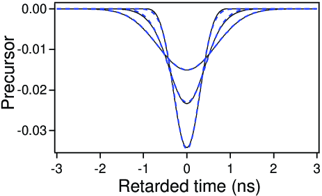
Figure 11: (Color online) Analytical forms of the precursor contribution to the signals of Fig. 10 (solid lines) and their best fit by Gaussians (dashed lines).

When the precursors are generated by a single discontinuity of the input signal, their shape in the asymptotic limit strongly depends on the order of this discontinuity. Equations (17), (21), (33), and (35) lead us to conjecture that the precursor has a Gaussian (Gaussian derivative) shape when the discontinuity order is odd (even). Complementary calculations made when $v(0,t)=\left(t/T_{r}\right)^{n}u_{H}(t)\sin\left(\omega_{c}t\right)$ or $\left(t/T_{r}\right)^{n}u_{H}(t)\cos\left(\omega_{c}t\right)$ for $n=2$ and $n=3$ support this conjecture but it should be remarked that the precursor amplitude is a rapidly decreasing function of $n$ .

The effect of the rise time of the input signal on the precursors is generally studied by considering input signals whose amplitude linearly increases during a time $T_{r}\leq T_{c}$ and is then maintained constant al89 ; sto01 ; ou09 ; ou12 . The corresponding complex signal may be written as

$$\tilde{v}_{L}(0,t)=\frac{t}{T_{r}}u_{H}(t)\,e^{i\omega_{c}t}\\ -e^{i\omega_{c}T_{r}}\frac{t-T_{r}}{T_{r}}u_{H}(t-T_{r})\,e^{i\omega_{c}(t-T_{r})}.$$ (36)

It generates the output signal

$$\tilde{v}_{L}(\ell,t)=\tilde{v}(\ell,t)-e^{i\omega_{c}T_{r}}\tilde{\,v}(\ell,t-T_{r}),$$ (37)

where $\tilde{v}(\ell,t)$ is given by Eq. (30). For $\beta\left(t-T_{r}\right)\gg\alpha_{c}\ell$, Eq. (37) is reduced to $\tilde{v}_{L}(\ell,t)=e^{-\alpha_{c}\ell}e^{i\omega_{c}t}$, as expected since the long-term behavior of the main signal should not depend on the rise time of the input signal. Remarkable behaviors are obtained in the asymptotic limit when $T_{r}=T_{c}$ and $T_{r}=T_{c}/2$. When $T_{r}=T_{c}$, the precursors generated by the first and second discontinuities of the slope of the input signal interfere nearly destructively and the output signal are again given by Eq. (25) where $\tilde{v}_{p}(\ell,t)$ is now given by Eq. (33) for $v(0,t)\propto\sin\left(\omega_{c}t\right)$ and by Eq. (35) for $v(0,t)\propto\cos\left(\omega_{c}t\right)$ . The output signals then reads as

$$v(\ell,\theta)=\frac{2\beta}{\omega_{c}^{3}\sqrt{\pi}}\frac{d^{2}}{d\theta^{2}}\left(e^{-\beta^{2}\theta^{2}}\right)\\ =-\frac{\left(1-2\beta^{2}\theta^{2}\right)e^{-\beta^{2}\theta^{2}}}{2\left(\alpha_{c}\ell\right)^{3/2}\sqrt{\pi}}$$ (38)

(amplitude $\propto\ell^{-3/2}$) in the former case and as

$$v(\ell,\theta)=-\frac{\beta}{\omega_{c}^{2}\sqrt{\pi}}\frac{d}{d\theta}\left(e^{-\beta^{2}\theta^{2}}\right)=\frac{\beta\theta\,e^{-\beta^{2}\theta^{2}}}{2\alpha_{c}\ell\sqrt{\pi}}$$ (39)

(amplitude $\propto 1/\ell$) in the latter case. In both cases, $\theta=t-T_{c}/2$ . When $T_{r}=T_{c}/2$, the two precursors interfere constructively. For $v(0,t)\propto\sin\left(\omega_{c}t\right)$ and $v(0,t)\propto\cos\left(\omega_{c}t\right)$, we respectively get

$$v(\ell,\theta)=\frac{4\beta}{\omega_{c}^{2}\pi^{3/2}}\,\frac{d}{d\theta}\left(e^{-\beta^{2}\theta^{2}}\right)=-\frac{2\beta\theta\,e^{-\beta^{2}\mathit{\theta}^{2}}}{\alpha_{c}\ell\pi^{3/2}}$$ (40)

(amplitude $\propto 1/\ell$) and

$$v(\ell,\theta)=-\frac{2\beta}{\omega_{c}\pi^{3/2}}\,e^{-\beta^{2}\theta^{2}}=-\frac{e^{-\beta^{2}\theta^{2}}}{\pi^{3/2}\sqrt{\alpha_{c}\ell}}$$ (41)

(amplitude $\propto\ell^{-1/2}$), with $\theta=t-T_{c}/4$ in both cases. Figure 12 shows the output signals given by Eqs. (37) combined with Eq. (30) in the four cases considered in this paragraph. The optical thickness $\alpha_{c}\ell=7$ has been chosen in order that the main signal is dominated by the precursor but remains visible. The precursors obtained at the asymptotic limit are given for reference. Though the asymptotic limit is not attained, they provide a reasonable approximation of the complete signals. Complementary simulations obviously show that as $\alpha_{c}\ell$ is larger, the fit of the output signals by the asymptotic form of the precursors is better. Signals as those shown Fig. 12 have been actually observed in the numerical experiments reported in Refs al89 ; sto01 ; ou09 ; ou12 but the fact that the precursor shape may be a Gaussian, a Gaussian first derivative or a Gaussian second derivative is either not clearly stated or completely overlooked. All these numerical simulations were made by using a trapezoidal modulation with the same rise and fall times and a plateau whose duration is much larger than that of the precursors.

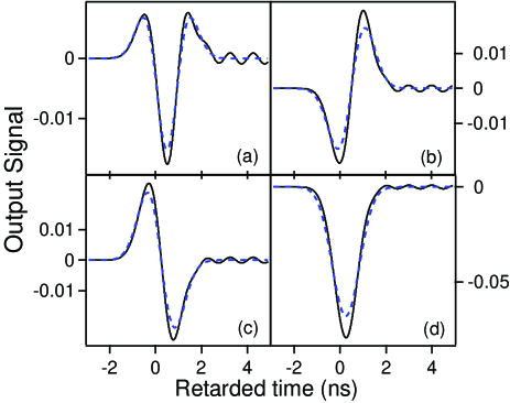
Figure 12: (Color online) Responses (solid line) to input signals with trapezoidal envelope of rise times $T_{r}=T_{c}$ or $T_{c}/2$ for $\alpha_{c}\ell=7$. (a) $T_{r}=T_{c}$, $v(0,t)\propto\sin(\omega_{c}t)$; (b) $T_{r}=T_{c}$, $v(0,t)\propto\cos(\omega_{c}t)$; (c) $T_{r}=T_{c}/2$, $v(0,t)\propto\sin(\omega_{c}t)$; and (d) $T_{r}=T_{c}/2$, $v(0,t)\propto\cos(\omega_{c}t)$ . The asymptotic solutions (dashed lines) are given for comparison.

As in the case of a rectangular modulation, depending on the plateau duration, the precursor and the postcursor may have the same or opposite signs al89 ; sto01 ; ou09 ; ou12 and even different shapes, e.g. a Gaussian associated with a Gaussian first-derivative or a Gaussian first derivative associated to a Gaussian second derivative. We incidentally remark that, by using a modulation with rise time, plateau duration and fall time all equal to $T_{c}$, it would theoretically be possible to generate a precursor with a Gaussian third derivative shape and an amplitude scaling as $1/\ell^{2}$. Calculations made in this case show that the corresponding precursor would emerge from the main field at distances where it would be too small to be detected in a real experiment.

V GENERAL ASYMPTOTIC PROPERTIES OF THE PRECURSORS

The shapes of the precursors obtained at the asymptotic limit and the dependence of their amplitude with the propagation distance (as $\ell^{-1/2}$, $\ell^{-1}$ or $\ell^{-3/2}$) are not specific to the input signals considered in the previous sections. As shown below they only result from the fact that, in the asymptotic limit, the width of the transfer function $H(\ell,\omega)$ is infinitely small compared to that of the Laplace-Fourier transform $V(0,\omega)$ of the input signal. The latter can then be developed in cumulants by keeping only the first of them. It reads as $V(0,\omega)=V(0,0)\,\mathrm{e}^{-i\omega t_{0}}=S_{0}e^{-i\omega t_{0}}$ where $S_{0}$ is the area of the input signal and $t_{0}$ its center of gravity re1 . We then get $V(\ell,\omega)=S_{0}H(\ell,\omega)e^{-i\omega t_{0}}$ and finally

$$v(\ell,t)=S_{0}\,h(t-t_{0})$$ (42)

This result, leading to a precursor amplitude scaling as $\ell^{-1/2}$, is general and applies in particular to the precursors given by Eqs. (17), (35), and (41), for which the input signals are such that $\left[S_{0},t_{0}\right]=\left[1/\omega_{c},0\right]$, $\left[-1/\left(\omega_{c}^{2}T_{r}\right),0\right]$ and $\left[-2/\left(\pi\omega_{c}\right),T_{c}/4\right]$, respectively.

The previous demonstration obviously fails when the input signal has a zero area. We consider in this case the first antiderivative of the input signal, namely ${}^{\left(1\right)}v(0,t)=\int_{-\infty}^{t}v(0,u_{1})\,du_{1}$, the Fourier transform of which reads as $V(0,\omega)/\left(i\omega\right)$. Repeating the previous procedure, we get $V(\ell,\omega)=\left(i\omega\right)S_{1}H(\ell,\omega)\mathrm{e}^{-i\omega t_{1}}$ and finally

$$v(\ell,t)=S_{1}\,\dot{h}(t-t_{1})$$ (43)

where $S_{1}$ and $t_{1}$ are the area and the center of gravity of ${}^{\left(1\right)}v(0,t)$ re1 . This general result, leading to a precursor amplitude scaling as $1/\ell$, applies in particular to the precursors given by Eqs. (21), (33), (39), and (40). The corresponding input signals are actually such that $S_{0}=0$ whereas $\left[S_{1},t_{1}\right]=\left[1/\omega_{c}^{2},0\right]$, $\left[2/\left(\omega_{c}^{3}T_{r}\right),0\right]$, $\left[-1/\omega_{c}^{2},T_{c}/2\right]$ and $\left[4/\left(\pi\omega_{c}^{2}\right),T_{c}/4\right]$, respectively.

When $S_{0}$ and $S_{1}$ are both zero, the same method is applied to the second antiderivative ${}^{\left(2\right)}v(0,t)=\int_{-\infty}^{t}\int_{-\infty}^{u_{2}}v(0,u_{1})\,du_{1}du_{2}$, the Fourier transform of which reads as $V(0,\omega)/\left(i\omega\right)^{2}$. Denoting $S_{2}$ as the area of ${}^{\left(2\right)}v(0,t)$ and $t_{2}$ as its center of gravity re1 , we finally get the output signal

$$v(\ell,t)=S_{2}\,\ddot{h}(t-t_{2})$$ (44)

the amplitude of which scales as $\ell^{-3/2}$. This result applies in particular to the precursors given by Eqs. (26) and (38). The second antiderivative of the corresponding input signals is such that $t_{2}=T_{c}/2$ in both cases, $S_{2}=2\pi/\omega_{c}^{3}$ in the first case and $S_{2}=2/\omega_{c}^{3}$ in the second case. According to Eq. (44), identical precursors will be thus obtained by amplifying the input signal in the second case by a factor $\pi$. This result is illustrated Fig. 13, which spectacularly shows that quite different input signals can generate the same precursor as long as they have the same integral properties.

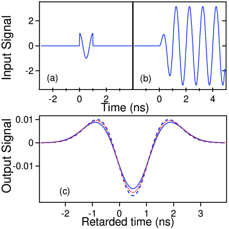
Figure 13: (Color online) Responses to the input signals (a) (solid line) and (b) (dashed line) for $\alpha_{c}\ell=12$. The asymptotic solution of Eq. (44) is given for comparison (dotted line).

Figure 13 has been drawn for a finite optical thickness ($\alpha_{c}\ell=12$) for which the precursors have sufficient amplitude and can be really observed. Both are close to the asymptotic form given by Eq. (44) from which they become undistinguishable for $\alpha_{c}\ell\geq 30$.

VI EFFECTS OF THE MEDIUM CONDUCTION

Debye media have always some conductivity. In the reference case of water, this conductivity $\sigma$ is essentially static in the radiofrequency and microwave domains ja98 ; ca09 and ranges from about $5\times 10^{-6}\,\mathrm{S/m}$ for ultrapure water (only due to $H^{+}$ and $OH^{-}$ ions) to $5\,\mathrm{S/m}$ for typical seawater (mainly due to dissolved salts). In the presence of conductivity, the complex refractive index reads as

$$\tilde{n}(\omega)=\sqrt{n_{\infty}^{2}+\frac{n_{0}^{2}-n_{\infty}^{2}}{1+i\omega\tau}+\frac{\sigma}{i\omega\varepsilon_{0}}}$$ (45)

When the conductivity is small enough, the main contribution to $\tilde{n}(\omega)$ and thus to $H(\ell,\omega)$ is expected to originate from frequencies such that the last term in Eq. (45) may be treated as a perturbation. Repeating the procedure that led to Eq. (6), we then get

$$\ln\left[H\left(\ell,\omega\right)\right]\approx-i\omega t_{B}-\frac{\omega^{2}}{4\beta^{2}}-\frac{\sigma\ell Z_{0}}{2},$$ (46)

where $Z_{0}=\sqrt{\mu_{0}/\left(n_{0}^{2}\varepsilon_{0}\right)}$ is the characteristic impedance of the medium at $\omega=0$ when $\sigma=0$. Using again a time retarded by $t_{B}$, we finally get the approximate transfer function $H_{a}(\ell,\omega)$

$$H_{a}(\ell,\omega)=\exp\left(-\frac{\sigma\ell Z_{0}}{2}\right)e^{-\frac{\omega^{2}}{4\beta^{2}}}$$ (47)

and the approximate impulse response $h_{a}\left(\ell,t\right)$

$$h_{a}\left(\ell,t\right)=\frac{\beta}{\sqrt{\pi}}\,e^{-\beta^{2}t^{2}}\exp\left(-\frac{\sigma\ell Z_{0}}{2}\right).$$ (48)

At this order of approximation, the effect of the medium conductivity is simply to reduce the impulse response and thus the response to any input signal by the factor $F=\exp\left(\frac{\sigma\ell Z_{0}}{2}\right)$. The effect of the medium conductivity will be negligible when the product of its conductance $\sigma\ell$ by its characteristic impedance $Z_{0}$ is small compared to $1$. For $\ell=1\,\mathrm{m}$, this condition is practically realized with ordinary drinking water whose typical conductivity ($10^{-3}\,\mathrm{S/m}$) leads to $F\approx 1.02$. The value $F=2$ is attained for $\sigma\approx 0.033\,\mathrm{S/m}$ and numerical simulations shows that $h_{a}\left(\ell,t\right)$ is then a very good approximation of the exact impulse response $h\left(\ell,t\right)$. We, however, note that the area of $h_{a}\left(\ell,t\right)$ is only $1/F$ whereas that of the exact impulse function remains equal to $1$. The reason for this apparent discrepancy is that the low frequencies, not fully taken into account in the previous calculation, originate a very small but very long tail whose area is the missing area. This tail is well visible on Fig. 14, obtained for $\sigma\approx 0.1\,\mathrm{S/m}$.

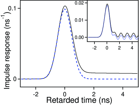
Figure 14: (Color online) Impulse response of water for $\ell=1\,\mathrm{m}$ ($t_{B}\approx 29.6\,\mathrm{ns}$) and $\sigma\approx 0.1\,\mathrm{S/m}$. The solid (dashed) line is the exact numerical result (our approximate analytical result). Inset: corresponding response to the canonical input signal $u_{H}(t)\sin\left(\omega_{c}t\right)$ with $\omega_{c}=2\pi\times 10^{9}\,\mathrm{s}^{-1}$.

Though $F$ is now as large as $8.3$, Eq. (48) continue to provide a good approximation of the main part of the impulse response. The inset of Fig. 14 shows the output signal generated by the canonical input signal $u_{H}(t)\sin\left(\omega_{c}t\right)$ with $\omega_{c}=2\pi\times 10^{9}\,\mathrm{s}^{-1}$ as previously. As expected, $v(\ell,t)$ is fairly well reproduced by the analytical expression $\mathrm{Im}\left[\tilde{v}(\ell,t)\right]/F$, where $\tilde{v}(\ell,t)$ is given by Eq. (10), and the long tail of $h\left(\ell,t\right)$ originates the upshift of the main signal.

Before considering the general case, it is instructive to examine the effects of the sole conductivity. This is achieved by neglecting the second term under the square root in Eq. (45). The transfer function is then reduced to $H_{c}(\ell,\omega)$ of the form

$$H_{c}(\ell,\omega)=\exp\left[-t_{\infty}\sqrt{\left(s+\gamma\right)^{2}-\gamma^{2}}\right],$$ (49)

where $s=i\omega$, $t_{\infty}=n_{\infty}\ell/c$ and $\gamma=\sigma/\left(2\varepsilon_{0}n_{\infty}^{2}\right)$. Using the inverse Laplace transform of $\exp\left[-t_{\infty}\sqrt{s^{2}-\gamma^{2}}\right]$ as given in Ref ab72 and translating $s$ by $\gamma$, we get the impulse response

$$h_{c}\left(\ell,t\right)=\gamma t_{\infty}\frac{\mathrm{I_{1}}\left(\gamma\,\sqrt{t^{2}-t_{\infty}^{2}}\right)}{\sqrt{t^{2}-t_{\infty}^{2}}}e^{-\gamma t}u_{H}(t-t_{\infty})\\ +e^{-\gamma t_{\infty}}\delta\left(t-t_{\infty}\right).$$ (50)

Here $\mathrm{I}_{1}(z)$ designates the first-order modified Bessel function and $t$ is the real time. A more rigorous demonstration of this result, showing its consistency with the boundary conditions, can be found in Ref lo94 . For $t^{2}\gg t_{\infty}^{2}$ and $\gamma t\gg 1$, Eq. (50) takes the asymptotic form

$$h_{c}\left(\ell,t\right)\approx\sqrt{\frac{\mu_{0}\sigma\ell^{2}}{4\pi t^{3}}}\exp\left(-\frac{\mu_{0}\sigma\ell^{2}}{4t}\right),$$ (51)

which is maximum for $t=t_{m}=\mu_{0}\sigma\ell^{2}/6$ with an amplitude

$$h_{m}=\sqrt{\frac{54}{\pi e^{3}}}\left(\frac{1}{\mu_{0}\sigma\ell^{2}}\right).$$ (52)

Coming back to the general problem, Eq. (48) is expected to provide a good approximation of the precursor if, at the time of its maximum, the ratio $R$ of $h_{a}\left(\ell,t\right)$ over $h_{c}\left(\ell,t\right)$is large. Using Eqs. (48) and (51) and taking into account that $n_{0}^{2}\gg n_{\infty}^{2}$, we get the approximate expression

$$R\approx n_{0}\sqrt{\frac{2\varepsilon_{0}}{\sigma\tau}}\exp\left(-\frac{Z_{0}\sigma\ell}{4}\right)=n_{0}\sqrt{\frac{2\varepsilon_{0}}{F\sigma\tau}}$$ (53)

In the conditions of the inset of Fig. 14 ($\ell=1\,\mathrm{m}$ , $\sigma\approx 0.1\,\mathrm{S/m}$.), $R$ was about $14$ and Eq.(48) actually provided a good approximation of the medium response to the canonical input signal with $\omega_{c}=2\pi\times 10^{9}\,\mathrm{s}^{-1}$ .

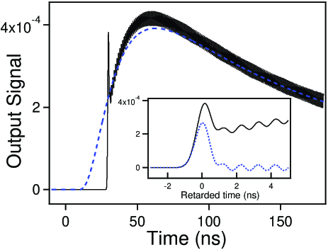
Figure 15: (Color online) Response to the canonical input signal for $\sigma\approx 0.3\,\mathrm{S/m}$ (other parameters as for the inset of Fig. 14). The solid (dashed) line is the exact numerical result (the analytical result obtained by considering the sole effects of conductivity). Inset: enlargement of the output signal around $t=t_{B}$. Here the dashed line is the analytical result derived from Eq. (48).

Figure 15 shows the result obtained for $\sigma\approx 0.3\,\mathrm{S/m}$, leading to $R\approx 1$. The response obtained by considering the sole effects of conductivity re2 approximates fairly well the mean value of the exact response for $t>t_{B}$. The coincidence becomes exact for $t\gg t_{B}$, the long-time behavior being mainly determined by the low frequencies where the conductivity term prevails on the polarization term in Eq. (45). On the other hand, the inset shows that the beginning of the response is perfectly reproduced by the analytical response derived from Eq. (48). Main signal and precursor obviously decrease with the conductivity. For $\sigma\approx 0.4\,\mathrm{S/m}$, the former remains visible whereas the latter appears as a slight overshot of amplitude about $10^{5}$ times smaller than that of the input signal and would be probably undetectable in a real experiment.

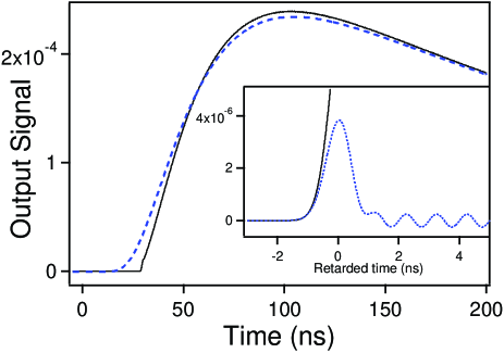
Figure 16: (Color online) Same as Fig. 15 for $\sigma\approx 0.5\,\mathrm{S/m}$. Note that the scales of the inset and the main figure are very different.

Figure 16 shows that main signal and precursor become practically invisible for $\sigma\approx 0.5\,\mathrm{S/m}$. The overall response is well fitted by the analytical function derived from Eq. (50) re2 but Eq. (48) continue to perfectly reproduce the very first beginning of the signal (inset). Finally, as the conductivity increases, the fit of the output signal by $h_{c}\left(\ell,t\right)/\omega_{c}$ improvies. Any trace of precursor then disappears and the response is reduced to a broad signal of amplitude (duration) scaling as $1/\ell^{2}$ (as $\ell^{2}$). See Eq. (51) and (52).

The simulations of Figs. 14 (inset), 15, and 16 have been made for $\ell=1\,\mathrm{m}$ and $\omega_{c}=2\pi\times 10^{9}\,\mathrm{s}^{-1}$. These parameters are those of a realistic experiment on water and, such that the Brillouin precursor generated by the canonical input signal predominates on the main field which remains visible. The analytical results are, however, general. They notably show that the validity domains of the low- and high-conductivity approximations are not entirely determined by the absolute value of the conductivity as considered in Ref ca09 but strongly depend on the propagation length. For example, a conductivity $\sigma\approx 3.3\times 10^{-2}\,\mathrm{S/m}$ suffices to be perfectly inside the low conductivity domain ($R\approx 51$) when $\ell=1\,\mathrm{m}$, whereas a conductivity as low as $\sigma\approx 1.72\times 10^{-3}\,\mathrm{S/m}$ is required to attain the same value of $R$ when $\ell=100\,\mathrm{m}$ . Note additionally that the amplitude-reduction factor $F$ is as large as $38$ in the latter case but $2$ in the former.

VII CONCLUSION

Sommerfeld and Brillouin precursors originate from interrelated effects of group-velocity dispersion and of frequency-dependent absorption of the medium. The former prevail in the formation of the Sommerfeld precursors som14 ; fa03 ; bm12 but both effects generally contribute to that of the Brillouin precursors bri14 ; bri32 ; bm12 . In Debye media, however, as soon as the Brillouin precursor is distinguishable from the main field, we have shown that the impulse response of the medium is perfectly fitted by the Gaussian obtained by neglecting the dispersion effects. By means of simple convolutions, we have then obtained explicit analytical expressions of the response of the medium to a wide class of input signals and extracted from them those of the precursor. Our main results are summarized below.

For input signals with a single initial discontinuity, the Brillouin precursor is well approximated by a Gaussian (Figs. 3 and 11) or a Gaussian derivative (Figs. 5 and 9), depending on the parity of the discontinuity order. This approximation is excellent in the case of the canonical input signal $u_{H}(t)\sin\left(\omega_{c}t\right)$ considered by Sommerfeld and Brillouin (Fig. 3) and an exact expression of the precursor amplitude is obtained in this case [Eq. (13)]. When the input signal has two successive discontinuities separated by one period of the carrier frequency, the quasi-destructive interference of the corresponding precursors may generate a unique precursor with a second-Gaussian-derivative shape (Figs. 7, 12a, and 13).

In the limit where the optical thickness of the medium at the carrier frequency is very large, the above-mentioned shapes of precursor are exact and the precursors are simply proportional to the impulse response, to its first or to its second derivative, with amplitude scaling with the propagation distance $\ell$ as $\ell^{-1/2}$, $\ell^{-1}$ and $\ell^{-3/2}$ respectively. These remarkable asymptotic properties are not specific to particular input signals but are common to the precursors generated by all the input signals having the same integral properties. The same precursor can thus be generated by quite different input signals (Fig. 13).

An eventual static conductivity of the medium does not affect significantly the shape of the output signal and in particular of the precursor when the parameter $R$ given Eq.(53) is large (low conductivity limit). The main effect of the conductivity is then an overall reduction of the medium response [see Eq. (48) and Fig. 14]. In the opposite case where $R\ll 1$ (high conductivity limit), the precursor disappears and the output signal is well approximated by the broad signal obtained by neglecting the polarization contribution, the amplitude of which scales as $\ell^{-2}$ [see Eq. (52) and Fig. 16].

The results obtained in our study cover various situations. Only the Brillouin precursor generated by the canonical input signal has been actually evidenced in real experiments sto01 . Our theoretical analysis is expected to stimulate complementary experimental works.

References

- (1) A. Sommerfeld, Ann. Phys. (Leipzig) 44, 177 (1914).
- (2) L. Brillouin, Ann. Phys. (Leipzig) 44, 203 (1914).
- (3) L. Brillouin, Comptes Rendus du Congrès International d’Electricité, Paris 1932 (Gauthier-Villars, Paris 1933), Vol.2, pp. 739-788.
- (4) L. Brillouin,Wave Propagation and Group Velocity (Academic Press, New York, 1960). Authorized translations in English of Ref som14 ; bri14 ; bri32 can be found in this book.
- (5) K.E. Oughstun, Electromagnetic and Optical Pulse Propagation 2 : Temporal Pulse Dynamics in Dispersive Attenuative Media (Springer, New York, 2009).
- (6) H. Jeong, U.L. Österberg, and T. Hansson, J. Opt. Soc. Am. B 26, 2455 (2009).
- (7) K.E. Oughstun, N.A. Cartwright, D.J. Gauthier, and H. Jeong, J. Opt. Soc. Am. B 27, 1664 (2010).
- (8) B. Macke and B. Ségard, J. Opt. Soc. Am. B 28, 450 (2011).
- (9) A. Ciarkowski, Int. J. Electron. Telecommun. 57, 251 (2011).
- (10) B. Macke and B. Ségard, Phys. Rev. A 86, 013837 (2012).
- (11) P. Pleshko and I. Palocz, Phys. Rev. Lett. 22, 1201 (1969).
- (12) J. Aaviksoo, J. Lippmaa, and J. Kuhl, J. Opt. Soc. Am. B 5, 1631 (1988).
- (13) B. Macke and B. Ségard, Phys. Rev. A 87, 043830 (2013).
- (14) B. Ségard, J. Zemmouri, and B. Macke, Europhys. Lett. 4, 47 (1987). See in particular Fig. 2 in this reference.
- (15) J. Aaviksoo, J. Kuhl, and K. Ploog, Phys. Rev. A 44, 5353(R) (1991).
- (16) H. Jeong, A. M. C. Dawes, and D. J. Gauthier, Phys. Rev. Lett. 96, 143901 (2006).
- (17) D. Wei, J.F. Chen, M.M.T. Loy, G.K.L. Wong, and S. Du, Phys. Rev. Lett. 103, 093602 (2009).
- (18) B. Macke and B. Ségard, Phys. Rev. A 81, 015803 (2010). See Fig. 1 in this paper.
- (19) Z.Q. Zhou, C.F. Li, and G.C. Guo, Phys. Rev. A 87, 045801 (2013).
- (20) E. Falcon, C. Laroche, and S. Fauve, Phys. Rev. Lett. 91, 064502 (2003).
- (21) P. Debye, Polar Molecules (Dover, New York 1929).
- (22) R. Albanese, J. Penn, and R. Medina, J. Opt. Soc. Am. A 6, 1441 (1989).
- (23) T.M. Roberts and P.G. Petropoulos, J. Opt. Soc. Am. A 13, 1204 (1996).
- (24) E.G. Farr and C.A. Frost, U.S Air Force, Laboratory Technical Report No. WL-TR-1997-7050, 1997. Available at http://www.dtic.mil/dtic/tr/fulltext/u2/a328788.pdf.
- (25) A. Karlsson and S. Rike, J. Opt. Soc. Am. A 15, 487 (1998).
- (26) Y. Liu and W. Wang, IEEE Trans. Electromagn. Compat. 43, 223 (2001).
- (27) D. C. Stoudt, F. E. Peterkin, and B. J. Hankla, NSWC Report No. JPOSTC-CRF-005-03, 2001. Available at http://ece-research.unm.edu/summa/notes/In/IN622.pdf.
- (28) T.M. Roberts, IEEE Trans. Antennas Propag. 52, 310 (2004).
- (29) K.E. Oughstun, IEEE Trans. Antennas Propag. 53, 1582 (2005).
- (30) M. Pieraccini, A. Bicci, D. Mecatti, G. Macaluso, and C. Atzeni, IEEE Trans. Antennas Propag. 57, 3612 (2009).
- (31) R. Safian, C.D. Sarris, and M. Mojahedi, IEEE Trans. Antennas Propag. 57, 3676 (2009).
- (32) M. Dawood, H.U.R. Mohammed, and A.V. Alejos, Electron. Lett. 46, 1645 (2010).
- (33) N. Cartwright, IEEE Trans. Antennas Propag. 59, 1571 (2011).
- (34) K.E. Oughstun and C.L. Palombini, in Proceedings of the International Microwave Symposium Digest (MTT), 2012 IEEE MTT-S International (IEEE, New York, 2012), pp. 1-3.
- (35) We use the definitions, sign conventions, and results of the linear system theory. See, for example, A.Papoulis, The Fourier Integral and Its Applications (Mc Graw Hill, New York, 1987).
- (36) D. Segelstein, M.S. Thesis, University of Missouri, Kansas City 1981 (unpublished). For a direct access to the relevant numerical data, see: http://www.philiplaven.com/Segelstein.txt
- (37) N.S. Bukhman, Quantum Electron. 34, 299 (2004).
- (38) Causality implies that for real time less than , that is for retarded time less than .
- (39) NIST Handbook of Mathematical functions, edited by F.W.J. Olver, D.W. Lozier, R.F. Boisvert, and C.W. Clark (Cambridge University Press, Cambridge, 2010).
- (40) The area (the center of gravity) is simply given by the first non-zero term (the following term) of the expansion of in power series of .
- (41) J.A. Jackson, Classical Electrodynamics, ed. (Wiley, New York, 1998).
- (42) N.A. Cartwright and K.E. Oughstun, Antennas and Propagation Society International Symposium, 2009. APSURSI ’09. IEEE (IEEE, Charleston, 2009) pp. 1-4.
- (43) Handbook of Mathematical Functions, edited by M. Abramowitz and I. A. Stegun (Dover, New York, 1972). See Eq.(29.3.96), p. 1027, in this book.
- (44) J. LoVetri and J.B. Ehrman, IEEE Trans. Electromagn. Compat. 36, 221 (1994). See Eq.(25) in this article, and the references cited therein.
- (45) evolving slowly at the scale of the period , this response is simply with and . See Eq. (42) and Ref re1 . Note also that the location and the amplitude of the maximum are in excellent agreement with those derived from the asymptotic form of .