Implementing Randomized Matrix Algorithms in Parallel and Distributed Environments

Abstract

In this era of large-scale data, distributed systems built on top of clusters of commodity hardware provide cheap and reliable storage and scalable processing of massive data. With cheap storage, instead of storing only currently-relevant data, it is common to store as much data as possible, hoping that its value can be extracted later. In this way, exabytes ($10^{18}$ bytes) of data are being created on a daily basis. Extracting value from these data however, requires scalable implementations of advanced analytical algorithms beyond simple data processing, e.g., statistical regression methods, linear algebra, and optimization algorithms. Many traditional methods are designed to minimize floating-point operations, which is the dominant cost of in-memory computation on a single machine. In parallel and distributed environments, however, load balancing and communication, including disk and network I/O, can easily dominate computation. These factors greatly increase the complexity of algorithm design and challenge traditional ways of thinking about the design of parallel and distributed algorithms.

Here, we review recent work on developing and implementing randomized matrix algorithms in large-scale parallel and distributed environments. Randomized algorithms for matrix problems have received a great deal of attention in recent years, thus far typically either in theory or in machine learning applications or with implementations on a single machine. Our main focus is on the underlying theory and practical implementation of random projection and random sampling algorithms for very large very overdetermined (i.e., overconstrained) $\ell_{1}$ and $\ell_{2}$ regression problems. Randomization can be used in one of two related ways: either to construct sub-sampled problems that can be solved, exactly or approximately, with traditional numerical methods; or to construct preconditioned versions of the original full problem that are easier to solve with traditional iterative algorithms. Theoretical results demonstrate that in near input-sparsity time and with only a few passes through the data one can obtain very strong relative-error approximate solutions, with high probability. Empirical results highlight the importance of various trade-offs (e.g., between the time to construct an embedding and the conditioning quality of the embedding, between the relative importance of computation versus communication, etc.) and demonstrate that $\ell_{1}$ and $\ell_{2}$ regression problems can be solved to low, medium, or high precision in existing distributed systems on up to terabyte-sized data.

1 Introduction

Matrix algorithms lie at the heart of many applications, both historically in areas such as signal processing and scientific computing as well as more recently in areas such as machine learning and data analysis. Essentially, the reason is that matrices provide a convenient mathematical structure with which to model data arising in a broad range of applications: an $m\times n$ real-valued matrix $A$ provides a natural structure for encoding information about $m$ objects, each of which is described by $n$ features. Alternatively, an $n\times n$ real-valued matrix $A$ can be used to describe the correlations between all pairs of $n$ data points, or the weighted edge-edge adjacency matrix structure of an $n$-node graph. In astronomy, for example, very small angular regions of the sky imaged at a range of electromagnetic frequency bands can be represented as a matrix—in that case, an object is a region and the features are the elements of the frequency bands. Similarly, in genetics, DNA SNP (Single Nucleotide Polymorphism) or DNA microarray expression data can be represented in such a framework, with $A_{ij}$ representing the expression level of the $i^{th}$ gene or SNP in the $j^{th}$ experimental condition or individual. Similarly, term-document matrices can be constructed in many Internet applications, with $A_{ij}$ indicating the frequency of the $j^{th}$ term in the $i^{th}$ document.

Most traditional algorithms for matrix problems are designed to run on a single machine, focusing on minimizing the number of floating-point operations per second (FLOPS). On the other hand, motivated by the ability to generate very large quantities of data in relatively automated ways, analyzing data sets of billions or more of records has now become a regular task in many companies and institutions. In a distributed computational environment, which is typical in these applications, communication costs, e.g., between different machines, are often much more important than computational costs. What is more, if the data cannot fit into memory on a single machine, then one must scan the records from secondary storage, e.g., hard disk, which makes each pass through the data associated with enormous I/O costs. Given that, in many of these large-scale applications, regression, low-rank approximation, and related matrix problems are ubiquitous, the fast computation of their solutions on large-scale data platforms is of interest.

In this paper, we will provide an overview of recent work in Randomized Numerical Linear Algebra (RandNLA) on implementing randomized matrix algorithms in large-scale parallel and distributed computational environments. RandNLA is a large area that applies randomization as an algorithmic resource to develop improved algorithms for regression, low-rank matrix approximation, and related problems [1]. To limit the presentation, here we will be most interested in very large very rectangular linear regression problems on up to terabyte-sized data: in particular, in the $\ell_{2}$ regression (also known as least squares, or LS) problem and its robust alternative, the $\ell_{1}$ regression (also known as least absolute deviations, LAD, or least absolute errors, LAE) problem, with strongly rectangular “tall” data. Although our main focus is on $\ell_{2}$ and $\ell_{1}$ regression, much of the underlying theory holds for $\ell_{p}$ regression, either for $p\in[1,2]$ or for all $p\in[1,\infty)$, and thus for simplicity we formulate many of our results in $\ell_{p}$.

Several important conclusions will emerge from our presentation.

• First, many of the basic ideas from RandNLA in RAM extend to RandNLA in parallel/distributed environments in a relatively straightforward manner, assuming that one is more concerned about communication than computation. This is important from an algorithm design perspective, as it highlights which aspects of these RandNLA algorithms are peculiar to the use of randomization and which aspects are peculiar to parallel/distributed environments.

• Second, with appropriate engineering of random sampling and random projection algorithms, it is possible to compute good approximate solutions—to low precision (e.g., $1$ or $2$ digits of precision), medium precision (e.g., $3$ or $4$ digits of precision), or high precision (e.g., up to machine precision)—to several common matrix problems in only a few passes over the original matrix on up to terabyte-sized data. While low precision is certainly appropriate for many data analysis and machine learning applications involving noisy input data, the appropriate level of precision is a choice for user of an algorithm to make; and there are obvious advantages to having the developer of an algorithm provide control to the user on the quality of the answer returned by the algorithm.

• Third, the design principles for developing high-quality RandNLA matrix algorithms depend strongly on whether one is interested in low, medium, or high precision. (An example of this is whether to solve the randomized subproblem with a traditional method or to use the randomized subproblem to create a preconditioned version of the original problem.) Understanding these principles, the connections between them, and how they relate to traditional principles of NLA algorithm design is important for providing high-quality implementations of recent theoretical developments in the RandNLA literature.

	$m$	$n$
SNP	number of SNPs ($10^{7}$)	number of subjects ($10^{3}$)
TinyImages	number of images ($10^{8}$)	number of pixels in each image ($10^{3}$)
PDE	number of degrees of freedom	number of time steps
sensor network	size of sensing data	number of sensors
NLP	number of words and $n$-grams	number of documents
tick data	number of ticks	number of stocks

Table 1: Examples of strongly rectangular datasets

Although many of the ideas we will discuss can be extended to related matrix problems such as low-rank matrix approximation, there are two main reasons for restricting attention to strongly rectangular data. The first, most obvious, reason is that strongly rectangular data arises in many fields to which machine learning and data analysis methods are routinely applied. Consider, e.g., Table 1, which lists a few examples.

• In genetics, single nucleotide polymorphisms (SNPs) are important in the study of human health. There are roughly $10$ million SNPs in the human genome. However, there are typically at most a few thousand subjects for a study of a certain type of disease, due to the high cost of determination of genotypes and limited number of target subjects.

• In Internet applications, strongly rectangular datasets are common. For example, the image dataset called TinyImages [2] which contains $80$ million images of size $32\times 32$ collected from Internet.

• In spatial discretization of high-dimensional partial differential equations (PDEs), the number of degrees of freedom grows exponentially as dimension increases. For 3D problems, it is common that the number of degrees of freedom reaches $10^{9}$, for example, by having a $1000\times 1000\times 1000$ discretization of a cubic domain. However, for a time-dependent problem, time stays one-dimensional. Though depending on spatial discretization (e.g., the Courant-Friedrichs-Lewy condition for hyperbolic PDEs), the number of time steps is usually much less than the number of degrees of freedoms in spatial discretization.

• In geophysical applications, especially in seismology, the number of sensors is much less than the number of data points each sensor collects. For example, Werner-Allen et al. [3] deployed three wireless sensors to monitor volcanic eruptions. In 54 hours, each sensor sent back approximately $20$ million packets.

• In natural language processing (NLP), the number of documents is much less than the number of $n$-grams, which grows geometrically as $n$ increases. For example, the webspam dataset contains 350,000 documents and 254 unigrams, but 680,715 trigrams.

• In high-frequency trading, the number of relevant stocks is much less than the number of ticks, changes to the best bid and ask. For example, in 2012 ISE Historical Options Tick Data has daily files with average size greater than 100GB uncompressed.

A second, less obvious, reason for restricting attention to strongly rectangular data is that many of the algorithmic methods that are developed for them (both the RandNLA methods we will review as well as deterministic NLA methods that have been used traditionally) have extensions to low-rank matrix approximation and to related problems on more general “fat” matrices. For example, many of the methods for SVD-based low-rank approximation and related rank-revealing QR decompositions of general matrices have strong connections to QR decomposition methods for rectangular matrices; and, similarly, many of the methods for more general linear and convex programming arise in special (e.g., $\ell_{1}$ regression) linear programming problems. Thus, they are a good problem class to consider the development of matrix algorithms (either in general or for RandNLA algorithms) in parallel and distributed environments.

It is worth emphasizing that the phrase “parallel and distributed” can mean quite different things to different research communities, in particular to what might be termed HPC (high performance computing) or scientific computing researchers versus data analytics or database or distributed data systems researchers. There are important technical and cultural differences here, but there are also some important similarities. For example, to achieve parallelism, one can use multi-threading on a shared-memory machine, or one can use message passing on a multi-node cluster. Alternatively, to process massive data on large commodity clusters, Google’s MapReduce [4] describes a computational framework for distributed computation with fault tolerance. For computation not requiring any internode communication, one can achieve even better parallelism. We don’t want to dwell on many of these important details here: this is a complicated and evolving space; and no doubt the details of the implementation of many widely-used algorithms will evolve as the space evolves. To give the interested reader a quick sense of some of these issues, though, here we provide a very high-level representative description of parallel environments and how they scale. As one goes down this list, one tends to get larger and larger.

name	cores	memory	notes
Shared memory	$[10,10^{3}]$	$[100\text{GB},100\text{TB}]$
Message passing	$[200,10^{5}]$	$[1\text{TB},1000\text{TB}]$	CUDA cores: $[5\times 10^{4},3\times 10^{6}]$
			GPU memory: $[500\text{GB},20\text{TB}]$
MapReduce	$[40,10^{5}]$	$[240\text{GB},100\text{TB}]$	storage: $[100\text{TB},100\text{PB}]$
Distributed computing	$[-,3\times 10^{5}]$

Table 2: High-level representative description of parallel environments.

In addition, it is also worth emphasizing that there is a great deal of related work in parallel and distributed computing, both in numerical linear algebra as well as more generally in scientific computing. For example, Valiant has provided a widely-used model for parallel computation [5]; Aggarwal et al. have analyzed the communication complexity of PRAMs [6]; Lint and Agerwala have highlighted communication issues that arise in the design of parallel algorithms [7]; Heller has surveyed parallel algorithms in numerical linear algebra [8]; Toledo has provided a survey of out-of-core algorithms in numerical linear algebra [9]; Ballard et al. have focused on developing algorithms for minimizing communication in numerical linear algebra [10]; and Bertsekas and Tsitsiklis have surveyed parallel and distributed iterative algorithms [11]. We expect that some of the most interesting developments in upcoming years will involve coupling the ideas for implementing RandNLA algorithms in parallel and distributed environments that we describe in this review with these more traditional ideas for performing parallel and distributed computation.

In the next section, Section 2, we will review the basic ideas underlying RandNLA methods, as they have been developed in the special case of $\ell_{2}$ regression in the RAM model. Then, in Section 3, we will provide notation, some background and preliminaries on $\ell_{2}$ and more general $\ell_{p}$ regression problems, as well as traditional methods for their solution. Then, in Section 4, we will describe rounding and embedding methods that are used in a critical manner by RandNLA algorithms; and in Section 5, we will review recent empirical results on implementing these ideas to solve up to terabyte-sized $\ell_{2}$ and $\ell_{1}$ regression problems. Finally, in Section 6, we will provide a brief discussion and conclusion. An overview of the general RandNLA area has been provided [1], and we refer the interested reader to this overview. In addition, two other reviews are available to the interested reader: an overview of how RandNLA methods can be coupled with traditional NLA algorithms for low-rank matrix approximation [12]; and an overview of how data-oblivious subspace embedding methods are used in RandNLA [13].

2 RandNLA in RAM

In this section, we will highlight several core ideas that have been central to prior work in RandNLA in (theory and/or practice in) RAM that we will see are also important as design principles for extending RandNLA methods to larger-scale parallel and distributed environments. We start in Section 2.1 by describing a prototypical example of a RandNLA algorithm for the very overdetermined LS problem; then we describe in Section 2.2 two problem-specific complexity measures that are important for low-precision and high-precision solutions to matrix problems, respectively, as well as two complementary ways in which randomization can be used by RandNLA algorithms; and we conclude in Section 2.3 with a brief discussion of running time considerations.

2.1 A meta-algorithm for RandNLA

A prototypical example of the RandNLA approach is given by the following meta-algorithm for very overdetermined LS problems [14, 1, 15, 16]. In particular, the problem of interest is to solve:

$$\min_{x}\|Ax-b\|_{2}.$$ (1)

The following meta-algorithm takes as input an $m\times n$ matrix $A$, where $m\gg n$, a vector $b$, and a probability distribution $\{\pi_{i}\}_{i=1}^{m}$, and it returns as output an approximate solution $\hat{x}$, which is an estimate of the exact answer $x^{*}$ of Problem (1).

• Randomly sampling. Randomly sample $r>n$ constraints, i.e., rows of $A$ and the corresponding elements of $b$, using $\{\pi_{i}\}_{i=1}^{m}$ as an importance sampling distribution.

• Subproblem construction. Rescale each sampled row/element by $1/(r\pi_{i})$ to form a weighted LS subproblem.

• Solving the subproblem. Solve the weighted LS subproblem, formally given in (2) below, and then return the solution $\hat{x}$.

It is convenient to describe this meta-algorithm in terms of a random “sampling matrix” $S$, in the following manner. If we draw $r$ samples (rows or constraints or data points) with replacement, then define an $r\times m$ sampling matrix, $S$, where each of the $r$ rows of $S$ has one non-zero element indicating which row of $A$ (and element of $b$) is chosen in a given random trial. In this case, the $(i,k)^{th}$ element of $S$ equals $1/\sqrt{r\pi_{k}}$ if the $k^{th}$ data point is chosen in the $i^{th}$ random trial (meaning, in particular, that every non-zero element of $S$ equals $\sqrt{n/r}$ for sampling uniformly at random). With this notation, this meta-algorithm constructs and solves the weighted LS estimator:

$$\hat{x}=\arg\min_{x}\|SAx-Sb\|_{2}.$$ (2)

Since this meta-algorithm samples constraints and not variables, the dimensionality of the vector $\hat{x}$ that solves the (still overconstrained, but smaller) weighted LS subproblem is the same as that of the vector $x^{*}$ that solves the original LS problem. The former may thus be taken as an approximation of the latter, where, of course, the quality of the approximation depends critically on the choice of $\{\pi_{i}\}_{i=1}^{n}$. Although uniform subsampling (with or without replacement) is very simple to implement, it is easy to construct examples where it will perform very poorly [14, 1, 16]. On the other hand, it has been shown that, for a parameter $\gamma\in(0,1]$ that can be tuned, if

$$\pi_{i}\geq\gamma\frac{h_{ii}}{p},\;\;\mbox{and }r=\operatorname{\mathcal{O}}(p\log(p)/(\gamma\epsilon^{2})),$$ (3)

where the so-called statistical leverage scores $h_{ii}$ are defined in (6) below, i.e., if one draws the sample according to an importance sampling distribution that is proportional to the leverage scores of $A$, then with constant probability (that can be easily boosted to probability $1-\delta$, for any $\delta>0$) the following relative-error bounds hold:

$$||b-A\hat{x}||_{2} \leq (1+\epsilon)||b-Ax^{*}||_{2}\hskip 5.69054pt\mbox{ and }$$ (4)

$$||x^{*}-\hat{x}||_{2} \leq \sqrt{\epsilon}\left(\kappa(A)\sqrt{\xi^{-2}-1}\right)||x^{*}||_{2},$$ (5)

where $\kappa(A)$ is the condition number of $A$ and where $\xi=||UU^{T}b||_{2}/||b||_{2}$ is a parameter defining the amount of the mass of $b$ inside the column space of $A$ [14, 1, 15].

Due to the crucial role of the statistical leverage scores in (3), this canonical RandNLA procedure has been referred to as the algorithmic leveraging approach to approximating LS approximation [16]. In addition, although this meta-algorithm has been described here only for very overdetermined LS problems, it generalizes to other linear regression problems and low-rank matrix approximation problems on less rectangular matrices [17, 18, 19, 20, 21].

2.2 Leveraging, conditioning, and using randomization

Leveraging and conditioning refer to two types of problem-specific complexity measures, i.e., quantities that can be computed for any problem instance that characterize how difficult that problem instance is for a particular class of algorithms. Understanding these, as well as different uses of randomization in algorithm design, is important for designing RandNLA algorithms, both in theory and/or practice in RAM as well as in larger parallel and distributed environments. For now, we describe these in the context of very overdetermined LS problems.

• Statistical leverage. (Related to eigenvectors; important for obtaining low-precision solutions.) If we let $H=A(A^{T}A)^{-1}A^{T}$, where the inverse can be replaced with the Moore-Penrose pseudoinverse if $A$ is rank deficient, be the projection matrix onto the column span of $A$, then the $i^{th}$ diagonal element of $H$,

  $$h_{ii}=A_{(i)}(A^{T}A)^{-1}A_{(i)}^{T},$$ (6)

  where $A_{(i)}$ is the $i^{th}$ row of $A$, is the statistical leverage of $i^{th}$ observation or sample. Since $H$ can alternatively be expressed as $H=UU^{T}$, where $U$ is any orthogonal basis for the column space of $X$, e.g., the $Q$ matrix from a QR decomposition or the matrix of left singular vectors from the thin SVD, the leverage of the $i^{th}$ observation can also be expressed as

  $$h_{ii}=\sum_{j=1}^{n}U_{ij}^{2}=||U_{(i)}||^{2},$$ (7)

  where $U_{(i)}$ is the $i^{th}$ row of $U$. Leverage scores provide a notion of “coherence” or “outlierness,” in that they measure how well-correlated the singular vectors are with the canonical basis [18, 15, 22] as well as which rows/constraints have largest “influence” on the LS fit [23, 24, 25, 26]. Computing the leverage scores $\{h_{ii}\}_{i=1}^{m}$ exactly is generally as hard as solving the original LS problem (but $1\pm\epsilon$ approximations to them can be computed more quickly, for arbitrary input matrices [15]).

  Leverage scores are important from an algorithm design perspective since they define the key nonuniformity structure needed to control the complexity of high-quality random sampling algorithms. In particular, naïve uniform random sampling algorithms perform poorly when the leverage scores are very nonuniform, while randomly sampling in a manner that depends on the leverage scores leads to high-quality solutions. Thus, in designing RandNLA algorithms, whether in RAM or in parallel-distributed environments, one must either quickly compute approximations to the leverage scores or quickly preprocess the input matrix so they are nearly uniformized—in which case uniform random sampling on the preprocessed matrix performs well.

  Informally, the leverage scores characterize where in the high-dimensional Euclidean space the (singular value) information in $A$ is being sent, i.e., how the quadratic well (with aspect ratio $\kappa(A)$ that is implicitly defined by the matrix $A$) “sits” with respect to the canonical axes of the high-dimensional Euclidean space. If one is interested in obtaining low-precision solutions, e.g., $\epsilon=10^{-1}$, that can be obtained by an algorithm that provides $1\pm\epsilon$ relative-error approximations for a fixed value of $\epsilon$ but whose $\epsilon$ dependence is polynomial in $1/\epsilon$, then the key quantities that must be dealt with are statistical leverage scores of the input data.

• Condition number. (Related to eigenvalues; important for obtaining high-precision solutions.) If we let $\sigma_{\max}(A)$ and $\sigma_{\min}(A)$ denote the largest and smallest nonzero singular values of $A$, respectively, then $\kappa(A)=\sigma_{\max}(A)/\sigma^{+}_{\min}(A)$ is the $\ell_{2}$-norm condition number of $A$ which is formally defined in Definition 3. Computing $\kappa(A)$ exactly is generally as hard as solving the original LS problem. The condition number $\kappa(A)$ is important from an algorithm design perspective since $\kappa(A)$ defines the key nonuniformity structure needed to control the complexity of high-precision iterative algorithms, i.e., it bounds the number of iterations needed for iterative methods to converge. In particular, for ill-conditioned problems, e.g., if $\kappa(A)\approx 10^{6}\gg 1$, then the convergence speed of iterative methods is very slow, while if $\kappa\gtrsim 1$ then iterative algorithms converge very quickly. Informally, $\kappa(A)$ defines the aspect ratio of the quadratic well implicitly defined by $A$ in the high-dimensional Euclidean space. If one is interested in obtaining high-precision solutions, e.g., $\epsilon=10^{-10}$, that can be obtained by iterating a low-precision solution to high precision with an iterative algorithm that converges as $\log(1/\epsilon)$, then the key quantity that must be dealt with is the condition number of the input data.

• Monte Carlo versus Las Vegas uses of randomization. Note that the guarantee provided by the meta-algorithm, as stated above, is of the following form: the algorithm runs in no more than a specified time $T$, and with probability at least $1-\delta$ it returns a solution that is an $\epsilon$-good approximation to the exact solution. Randomized algorithms that provide guarantees of this form, i.e., with running time that is is deterministic, but whose output may be incorrect with a certain small probability, are known as Monte Carlo algorithms [27]. A related class of randomized algorithms, known as Las Vegas algorithms, provide a different type of guaranatee: they always produce the correct answer, but the amount of time they take varies randomly [27]. In many applications of RandNLA algorithms, guarantees of this latter form are preferable.

The notions of condition number and leverage scores have been described here only for very overdetermined $\ell_{2}$ regression problems. However, as discussed in Section 3 below (as well as previously [17, 19]), these notions generalize to very overdetermined $\ell_{p}$, for $p\neq 2$, regression problems [19] as well as to $p=2$ for less rectangular matrices, as long as one specifies a rank parameter $k$ [17]. Understanding these generalizations, as well as the associated tradeoffs, will be important for developing RandNLA algorithms in parallel and distributed environments.

2.3 Running Time Considerations in RAM

As presented, the meta-algorithm of the previous subsection has a running time that depends on both the time to construct the probability distribution, $\{\pi_{i}\}_{i=1}^{n}$, and the time to solve the subsampled problem. For uniform sampling, the former is trivial and the latter depends on the size of the subproblem. For estimators that depend on the exact or approximate (recall the flexibility in (3) provided by $\gamma$) leverage scores, the running time is dominated by the exact or approximate computation of those scores. A naïve algorithm involves using a QR decomposition or the thin SVD of $A$ to obtain the exact leverage scores. This naïve implementation of the meta-algorithm takes roughly $\operatorname{\mathcal{O}}(mn^{2}/\epsilon)$ time and is thus no faster (in the RAM model) than solving the original LS problem exactly [14, 17]. There are two other potential problems with practical implementations of the meta-algorithm: the running time dependence of roughly $\operatorname{\mathcal{O}}(mn^{2}/\epsilon)$ time scales polynomially with $1/\epsilon$, which is prohibitive if one is interested in moderately small (e.g., $10^{-4}$) to very small (e.g., $10^{-10}$) values of $\epsilon$; and, since this is a randomized Monte Carlo algorithm, with some probability $\delta$ the algorithm might completely fail.

Importantly, all three of these potential problems can be solved to yield improved variants of the meta-algorithm.

• Making the algorithm fast: improving the dependence on $m$ and $n$. We can make this meta-algorithm “fast” in worst-case theory in RAM [28, 29, 14, 15, 20]. In particular, this meta-algorithm runs in $\operatorname{\mathcal{O}}(mn\log n/\epsilon)$ time in RAM if one does either of the following: if one performs a Hadamard-based random random projection and then performs uniform sampling in the randomly rotated basis [28, 29] (which, recall, is basically what random projection algorithms do when applied to vectors in a Euclidean space [1]); or if one quickly computes approximations to the statistical leverage scores (using the algorithm of [15], the running time bottleneck of which is applying a random projection to the input data) and then uses those approximate scores as an importance sampling distribution [14, 15]. In addition, by using carefully-constructed extremely-sparse random projections, both of these two approaches can be made to run in so-called “input sparsity time,” i.e., in time proportional to the number of nonzeros in the input data, plus lower-order terms that depend on the lower dimension of the input matrix [20].

• Making the algorithm high-precision: improving the dependence on $\epsilon$. We can make this meta-algorithm “fast” in practice, e.g., in “high precision” numerical implementation in RAM [30, 31, 32, 33]. In particular, this meta-algorithm runs in $\operatorname{\mathcal{O}}(mn\log n\log(1/\epsilon))$ time in RAM if one uses the subsampled problem constructed by the random projection/sampling process to construct a preconditioner, using it as a preconditioner for a traditional iterative algorithm on the original full problem [30, 31, 32]. This is important since, although the worst-case theory holds for any fixed $\epsilon$, it is quite coarse in the sense that the sampling complexity depends on $\epsilon$ as $1/\epsilon$ and not $\log(1/\epsilon)$. In particular, this means that obtaining high-precision with (say) $\epsilon=10^{-10}$ is not practically possible. In this iterative use case, there are several tradeoffs: e.g., one could construct a very high-quality preconditioner (e.g., using a number of samples that would yield a $1+\epsilon$ error approximation if one solved the LS problem on the subproblem) and perform fewer iterations, or one could construct a lower quality preconditioner by drawing many fewer samples and perform a few extra iterations. Here too, the input sparsity time algorithm of [20] could be used to improve the running time still further.

• Dealing with the $\delta$ failure probability. Although fixing a failure probability $\delta$ is convenient for theoretical analysis, in certain applications having even a very small probability that the algorithm might return a completely meaningless answer is undesirable. In this case, one is interested in converting a Monte Carlo algorithm into a Las Vegas algorithm. Fortuitously, those application areas, e.g., scientific computing, are often more interested in moderate to high precision solutions than in low precision solutions. In these case, using the subsampled problem to create a preconditioner for iterative algorithms on the original problem has the side effect that one changes a “fixed running time but might fail” algorithm to an “expected running time but will never fail” algorithm.

From above, we can make the following conclusions. The “fast in worst-case theory” variants of our meta-algorithm ([28, 29, 14, 15, 20]) represent qualitative improvements to the $\operatorname{\mathcal{O}}(mn^{2})$ worst-case asymptotic running time of traditional algorithms for the LS problem going back to Gaussian elimination. The “fast in numerical implementation” variants of the meta-algorithm ([30, 31, 32]) have been shown to beat Lapack’s direct dense least-squares solver by a large margin on essentially any dense tall matrix, illustrating that the worst-case asymptotic theory holds for matrices as small as several thousand by several hundred [31].

While these results are a remarkable success for RandNLA in RAM, they leave open the question of how these RandNLA methods perform in larger-scale parallel/distributed environments, and they raise the question of whether the same RandNLA principles can be extended to other common regression problems. In the remainder of this paper, we will review recent work showing that if one wants to solve $\ell_{2}$ regression problems in parallel/distributed environments, and if one wants to solve $\ell_{1}$ regression problems in theory or in RAM or in parallel/distributed environments, then one can use the same RandNLA meta-algorithm and design principles. Importantly, though, depending on the exact situation, one must instantiate the same algorithmic principles in different ways, e.g., one must worry much more about communication rather than FLOPS.

3 Preliminaries on $\ell_{p}$ regression problems

In this section, we will start in Section 3.1 with a brief review of notation that we will use in the remainder of the paper. Then, in Sections 3.2, 3.3, and 3.4, we will review $\ell_{p}$ regression problems and the notions of condition number and preconditioning for these problems. Finally, in Sections 3.5 and 3.6, we will review traditional deterministic solvers for $\ell_{2}$ as well as $\ell_{1}$ and more general $\ell_{p}$ regression problems.

3.1 Notation conventions

We briefly list the notation conventions we follow in this work:

• We use uppercase letters to denote matrices and constants, e.g., $A$, $R$, $C$, etc.

• We use lowercase letters to denote vectors and scalars, e.g., $x$, $b$, $p$, $m$, $n$, etc.

• We use $\|\cdot\|_{p}$ to denote the $\ell_{p}$ norm of a vector, $\|\cdot\|_{2}$ the spectral norm of a matrix, $\|\cdot\|_{F}$ the Frobenius norm of a matrix, and $|\cdot|_{p}$ the element-wise $\ell_{p}$ norm of a matrix.

• We use uppercase calligraphic letters to denote point sets, e.g., $\mathcal{A}$ for the linear subspace spanned by $A$’s columns, $\mathcal{C}$ for a convex set, and $\mathcal{E}$ for an ellipsoid, except that $\operatorname{\mathcal{O}}$ is used for big O-notation.

• The “$\tilde{\ }$” accent is used for sketches of matrices, e.g., $\tilde{A}$, the “^∗” superscript is used for indicating optimal solutions, e.g., $x^{*}$, and the “$\hat{\ }$” accent is used for estimates of solutions, e.g., $\hat{x}$.

3.2 $\ell_{p}$ regression problems

In this work, a parameterized family of linear regression problems that is of particular interest is the $\ell_{p}$ regression problem.

Definition 1 ($\ell_{p}$ regression)

Given a matrix $A\in\operatorname{\mathbb{R}}^{m\times n}$, a vector $b\in\operatorname{\mathbb{R}}^{m}$, and $p\in[1,\infty]$, the $\ell_{p}$ regression problem specified by $A$, $b$, and $p$ is the following optimization problem:

$$\mathrm{minimize}_{x\in\operatorname{\mathbb{R}}^{n}}~{}\|Ax-b\|_{p},$$ (8)

where the $\ell_{p}$ norm of a vector $x$ is $\|x\|_{p}=\left(\sum_{i}|x_{i}|^{p}\right)^{1/p}$, defined to be $\max_{i}|x_{i}|$ for $p=\infty$. We call the problem strongly over-determined if $m\gg n$, and strongly under-determined if $m\ll n$.

Important special cases include the $\ell_{2}$ regression problem, also known as linear least squares (LS), and the $\ell_{1}$ regression problem, also known as least absolute deviations (LAD) or least absolute errors (LAE). The former is ubiquitous; and the latter is of particular interest as a robust regression technique, in that it is less sensitive to the presence of outliers than the former.

For general $p\in[1,\infty]$, denote $\operatorname{\mathcal{X}}^{*}$ the set of optimal solutions to (8). Let $x^{*}\in\operatorname{\mathcal{X}}^{*}$ be an arbitrary optimal solution, and let $f^{*}=\|Ax^{*}-b\|_{p}$ be the optimal objective value. We will be particularly interested in finding a relative-error approximation, in terms of the objective value, to the general $\ell_{p}$ regression problem (8).

Definition 2 (Relative-error approximation)

Given an error parameter $\epsilon>0$, $\hat{x}\in\operatorname{\mathbb{R}}^{n}$ is a $(1+\epsilon)$-approximate solution to the $\ell_{p}$ regression problem (8) if and only if

$$\hat{f}=\|A\hat{x}-b\|_{p}\leq(1+\epsilon)f^{*}.$$

In order to make our theory and our algorithms for general $\ell_{p}$ regression simpler more concise, we can use an equivalent formulation of (8) in our discussion.

$$\mathrm{minimize}_{x\in\operatorname{\mathbb{R}}^{n}} \|Ax\|_{p}$$ (9)

$$\mathrm{subject~{}to} c^{T}x=1.$$

Above, the “new” $A$ is $A$ concatenated with $-b$, i.e., $\begin{pmatrix}A&-b\end{pmatrix}$ and $c$ is a vector with a $1$ at the last coordinate and zeros elsewhere, i.e., $c\in\operatorname{\mathbb{R}}^{d+1}$ and $c=\begin{pmatrix}0&\ldots&0&1\end{pmatrix}$, to force the last element of any feasible solution to be $1$. We note that the same formulation is also used by [34] for solving unconstrained convex problems in relative scale. This formulation of $\ell_{p}$ regression, which consists of a homogeneous objective and an affine constraint, can be shown to be equivalent to the formulation of (8).

Consider, next, the special case $p=2$. If, in the LS problem

$$\text{minimize}_{x\in\mathbb{R}^{n}}\quad\|Ax-b\|_{2},$$ (10)

we let $r=\operatorname{rank}(A)\leq\min(m,n)$, then recall that if $r<n$ (the LS problem is under-determined or rank-deficient), then (10) has an infinite number of minimizers. In that case, the set of all minimizers is convex and hence has a unique element having minimum length. On the other hand, if $r=n$ so the problem has full rank, there exists only one minimizer to (10) and hence it must have the minimum length. In either case, we denote this unique min-length solution to (10) by $x^{*}$, and we are interested in computing $x^{*}$ in this work. This was defined in Problem (1) above. In this case, we will also be interested in bounding $\|x^{*}-\hat{x}\|_{2}$, for arbitrary or worst-case input, where $\hat{x}$ was defined in Problem (2) above and is an approximation to $x^{*}$.

3.3 $\ell_{p}$-norm condition number

An important concept in $\ell_{2}$ and more general $\ell_{p}$ regression problems, and in developing efficient algorithms for their solution, is the concept of condition number. For linear systems and LS problems, the $\ell_{2}$-norm condition number is already a well-established term.

Definition 3 ($\ell_{2}$-norm condition number)

Given a matrix $A\in\operatorname{\mathbb{R}}^{m\times n}$ with full column rank, let $\sigma^{\max}_{2}(A)$ be the largest singular value and $\sigma^{\min}_{2}(A)$ be the smallest singular value of $A$. The $\ell_{2}$-norm condition number of $A$ is defined as $\kappa_{2}(A)=\sigma^{\max}_{2}(A)/\sigma^{\min}_{2}(A)$. For simplicity, we use $\kappa_{2}$, $\sigma_{2}^{\min}$, and $\sigma_{2}^{\max}$ when the underlying matrix is clear from context.

For general $\ell_{p}$ norm and general $\ell_{p}$ regression problems, here we state here two related notions of condition number and then a lemma that characterizes the relationship between them.

Definition 4 ($\ell_{p}$-norm condition number (Clarkson et al. [19]))

Given a matrix $A\in\operatorname{\mathbb{R}}^{m\times n}$ and $p\in[1,\infty]$, let

$$\sigma_{p}^{\max}(A)=\max_{\|x\|_{2}=1}\|Ax\|_{p}\text{ and }\sigma_{p}^{\min}(A)=\min_{\|x\|_{2}=1}\|Ax\|_{p}.$$

Then, we denote by $\kappa_{p}(A)$ the $\ell_{p}$-norm condition number of $A$, defined to be:

$$\kappa_{p}(A)=\sigma_{p}^{\max}(A)/\sigma_{p}^{\min}(A).$$

For simplicity, we use $\kappa_{p}$, $\sigma_{p}^{\min}$, and $\sigma_{p}^{\max}$ when the underlying matrix is clear.

Definition 5 ($(\alpha,\beta,p)$-conditioning (Dasgupta et al. [35]))

Given a matrix $A\in\operatorname{\mathbb{R}}^{m\times n}$ and $p\in[1,\infty]$, let $\|\cdot\|_{q}$ be the dual norm of $\|\cdot\|_{p}$. Then $A$ is $(\alpha,\beta,p)$-conditioned if (1) $|A|_{p}\leq\alpha$, and (2) for all $z\in\operatorname{\mathbb{R}}^{n}$, $\|z\|_{q}\leq\beta\|Az\|_{p}$. Define $\bar{\kappa}_{p}(A)$, the $(\alpha,\beta,p)$-condition number of $A$, as the minimum value of $\alpha\beta$ such that $A$ is $(\alpha,\beta,p)$-conditioned. We use $\bar{\kappa}_{p}$ for simplicity if the underlying matrix is clear.

Lemma 1 (Equivalence of $\kappa_{p}$ and $\bar{\kappa}_{p}$ (Clarkson et al. [19]))

Given a matrix $A\in\operatorname{\mathbb{R}}^{m\times n}$ and $p\in[1,\infty]$, we always have

$$n^{-|1/2-1/p|}\kappa_{p}(A)\leq\bar{\kappa}_{p}(A)\leq n^{\max\{1/2,1/p\}}\kappa_{p}(A).$$

That is, by Lemma 1, if $m\gg n$, then the notions of condition number provided by Definition 4 and Definition 5 are equivalent, up to low-dimensional factors. These low-dimensional factors typically do not matter in theoretical formulations of the problem, but they can matter in practical implementations.

The $\ell_{p}$-norm condition number of a matrix can be arbitrarily large. Given the equivalence established by Lemma 1, we say that a matrix $A$ is well-conditioned in the $\ell_{p}$ norm if $\kappa_{p}$ or $\bar{\kappa}_{p}=\operatorname{\mathcal{O}}(\operatorname{poly}(n))$, independent of the high dimension $m$. We see in the following sections that the condition number plays a very important part in the analysis of traditional algorithms.

3.4 Preconditioning $\ell_{p}$ regression problems

Preconditioning refers to the application of a transformation, called the preconditioner, to a given problem instance such that the transformed instance is more-easily solved by a given class of algorithms. Most commonly, the preconditioned problem is solved with an iterative algorithm, the complexity of which depends on the condition number of the preconditioned problem.

To start, consider $p=2$, and recall that for a square linear system $Ax=b$ of full rank, this preconditioning usually takes one of the following forms:

left preconditioning $$\quad M^{\raisebox{0.62997pt}{\hbox{\tiny$T$}}}Ax=M^{\raisebox{0.62997pt}{\hbox{\tiny$T$}}}b,$$

right preconditioning $$\quad ANy=b,~{}x=Ny,$$

left and right preconditioning $$\quad M^{\raisebox{0.62997pt}{\hbox{\tiny$T$}}}ANy=M^{\raisebox{0.62997pt}{\hbox{\tiny$T$}}}b,~{}x=Ny.$$

Clearly, the preconditioned system is consistent with the original one, i.e., has the same $x^{*}$ as the unique solution, if the preconditioners $M$ and $N$ are nonsingular.

For the general LS Problem (1), more care should be taken so that the preconditioned system has the same min-length solution as the original one. In particular, if we apply left preconditioning to the LS problem $\min_{x}\|Ax-b\|_{2}$, then the preconditioned system becomes $\min_{x}\|M^{\raisebox{0.62997pt}{\hbox{\tiny$T$}}}Ax-M^{\raisebox{0.62997pt}{\hbox{\tiny$T$}}}b\|_{2}$, and its min-length solution is given by

$$x^{*}_{\text{left}}=(M^{\raisebox{0.62997pt}{\hbox{\tiny$T$}}}A)^{\dagger}M^{\raisebox{0.62997pt}{\hbox{\tiny$T$}}}b.$$

Similarly, the min-length solution to the right preconditioned system is given by

$$x^{*}_{\text{right}}=N(AN)^{\dagger}b.$$

The following lemma states the necessary and sufficient conditions for $A^{\dagger}=N(AN)^{\dagger}$ or $A^{\dagger}=(M^{\raisebox{0.62997pt}{\hbox{\tiny$T$}}}A)^{\dagger}M^{\raisebox{0.62997pt}{\hbox{\tiny$T$}}}$ to hold. Note that these conditions holding certainly imply that $x_{\text{right}}^{*}=x^{*}$ and $x_{\text{left}}^{*}=x^{*}$, respectively.

Lemma 2 (Left and right preconditioning (Meng et al. [32])

Given $A\in\mathbb{R}^{m\times n}$, $N\in\mathbb{R}^{n\times p}$ and $M\in\mathbb{R}^{m\times q}$, we have

1. $A^{\dagger}=N(AN)^{\dagger}$ if and only if $\text{range}(NN^{\raisebox{0.62997pt}{\hbox{\tiny$T$}}}A^{\raisebox{0.62997pt}{\hbox{\tiny$T$}}})=\text{range}(A^{\raisebox{0.62997pt}{\hbox{\tiny$T$}}})$,

2. $A^{\dagger}=(M^{\raisebox{0.62997pt}{\hbox{\tiny$T$}}}A)^{\dagger}M^{\raisebox{0.62997pt}{\hbox{\tiny$T$}}}$ if and only if $\text{range}(MM^{\raisebox{0.62997pt}{\hbox{\tiny$T$}}}A)=\text{range}(A)$.

Given this preconditioned problem, (13) (see below) bounds the number of itrations for certain iterative algorithms for the LS problem.

Just as with $p=2$, for more general $\ell_{p}$ regression problems with matrix $A\in\operatorname{\mathbb{R}}^{m\times n}$ with full column rank, although its condition numbers $\kappa_{p}(A)$ and $\bar{\kappa}_{p}(A)$ can be arbitrarily large, we can often find a matrix $R\in\operatorname{\mathbb{R}}^{n\times n}$ such that $AR^{-1}$ is well-conditioned. (This is not the $R$ from a QR decomposition of $A$, unless $p=2$, but some other matrix $R$.) In this case, the $\ell_{p}$ regression Problem (9) is equivalent to the following well-conditioned problem:

$$\text{minimize}_{y\in\operatorname{\mathbb{R}}^{n}} \|AR^{-1}y\|_{p},$$ (11)

subject to $$c^{T}R^{-1}y=1.$$

Clearly, if $y^{*}$ is an optimal solution to (11), then $x^{*}=R^{-1}y$ is an optimal solution to (9), and vice versa; however, (11) may be easier to solve than (9) because of better conditioning.

Since we want to reduce the condition number of a problem instance via preconditioning, it is natural to ask what the best possible outcome would be in theory. For $p=2$, an orthogonal matrix, e.g., the matrix $Q$ computed from a QR decomposition, has $\kappa_{2}(Q)=1$. More generally, for the $\ell_{p}$-norm condition number $\kappa_{p}$, we have the following existence result.

Lemma 3

Given a matrix $A\in\operatorname{\mathbb{R}}^{m\times n}$ with full column rank and $p\in[1,\infty]$, there exist a matrix $R\in\operatorname{\mathbb{R}}^{n\times n}$ such that $\kappa_{p}(AR^{-1})\leq n^{1/2}$.

This is a direct consequence of John’s theorem [36] on ellipsoidal rounding of centrally symmetric convex sets. For the $(\alpha,\beta,p)$-condition number $\bar{\kappa}_{p}$, we have the following lemma.

Lemma 4

Given a matrix $A\in\operatorname{\mathbb{R}}^{m\times n}$ with full column rank and $p\in[1,\infty]$, there exist a matrix $R\in\operatorname{\mathbb{R}}^{n\times n}$ such that $\bar{\kappa}_{p}(AR^{-1})\leq n$.

Note that Lemmas 3 and 4 are both existential results. Unfortunately, except the case when $p=2$, no polynomial-time algorithm is known that can provide such preconditioning for general matrices. Below, in Section 4, we will discuss two practical approaches for $\ell_{p}$-norm preconditioning: via ellipsoidal rounding and via subspace embedding, as well as subspace-preserving sampling algorithms built on top of them.

3.5 Traditional solvers for $\ell_{2}$ regression

Least squares is a classic problem in linear algebra. It has a long history, tracing back to Gauss, and it arises in numerous applications. A detailed survey of numerical algorithms for least squares is certainly beyond the scope of this work. In this section, we briefly describe some well-known direct methods and iterative methods that compute the min-length solution to a possibly rank-deficient least squares problem, and we refer readers to Björck [37] for additional details.

Direct methods

It is well known that the min-length solution of a least squares problem can be computed using the singular value decomposition (SVD). Let $A=U\Sigma V^{\raisebox{0.62997pt}{\hbox{\tiny$T$}}}$ be the compact SVD, where $U\in\operatorname{\mathbb{R}}^{m\times r}$, $\Sigma\in\operatorname{\mathbb{R}}^{r\times r}$, and $V\in\operatorname{\mathbb{R}}^{n\times r}$, i.e., only singular vectors corresponding to the non-zero singular values are calculated. We have $x^{*}=V\Sigma^{-1}U^{\raisebox{0.62997pt}{\hbox{\tiny$T$}}}b$. The matrix $V\Sigma^{-1}U^{\raisebox{0.62997pt}{\hbox{\tiny$T$}}}$ is the Moore-Penrose pseudoinverse of $A$, denoted by $A^{\dagger}$, which is defined and unique for any matrix. Hence we can simply write $x^{*}=A^{\dagger}b$. The SVD approach is accurate and robust to rank-deficiency.

Another way to solve a least squares problem is using complete orthogonal factorization. If we can find orthonormal matrices $Q\in\operatorname{\mathbb{R}}^{m\times r}$ and $Z\in\operatorname{\mathbb{R}}^{n\times r}$, and a matrix $T\in\operatorname{\mathbb{R}}^{r\times r}$, such that $A=QTZ^{\raisebox{0.62997pt}{\hbox{\tiny$T$}}}$, then the min-length solution is given by $x^{*}=ZT^{-1}Q^{\raisebox{0.62997pt}{\hbox{\tiny$T$}}}b$. We can treat SVD as a special case of complete orthogonal factorization. In practice, complete orthogonal factorization is usually computed via rank-revealing QR factorizations, making $T$ a triangular matrix. The QR approach is less expensive than SVD, but it is slightly less robust at determining the rank.

A third way to solve a least squares problem is by computing the min-length solution to the normal equation $A^{\raisebox{0.62997pt}{\hbox{\tiny$T$}}}Ax=A^{\raisebox{0.62997pt}{\hbox{\tiny$T$}}}b$, namely

$$x^{*}=(A^{\raisebox{0.62997pt}{\hbox{\tiny$T$}}}A)^{\dagger}A^{\raisebox{0.62997pt}{\hbox{\tiny$T$}}}b=A^{\raisebox{0.62997pt}{\hbox{\tiny$T$}}}(AA^{\raisebox{0.62997pt}{\hbox{\tiny$T$}}})^{\dagger}b.$$ (12)

It is easy to verify the correctness of (12) by replacing $A$ by its compact SVD $U\Sigma V^{\raisebox{0.62997pt}{\hbox{\tiny$T$}}}$. If $r=\min(m,n)$, a Cholesky factorization of either $A^{\raisebox{0.62997pt}{\hbox{\tiny$T$}}}A$ (if $m\geq n$) or $AA^{\raisebox{0.62997pt}{\hbox{\tiny$T$}}}$ (if $m\leq n$) solves (12). If $r<\min(m,n)$, we need the eigensystem of $A^{\raisebox{0.62997pt}{\hbox{\tiny$T$}}}A$ or $AA^{\raisebox{0.62997pt}{\hbox{\tiny$T$}}}$ to compute $x^{*}$. The normal equation approach is the least expensive among the three direct approaches we have mentioned, but it is also the least accurate one, especially on ill-conditioned problems. See Chapter 5 of Golub and Van Loan [38] for a detailed analysis. A closely related direct solver is the semi-normal equation method. It is often useful when the $R$-factor of the QR decomposition is known; see [39] for more details.

For sparse least squares problems, by pivoting $A$’s columns and rows, we may find a sparse factorization of $A$, which is preferred to a dense factorization for more efficient storage. For sparse direct methods, we refer readers to Davis [40].

Iterative methods

Instead of direct methods, we can use iterative methods to solve (10). If all the iterates $\{x^{(k)}\}$ are in $\text{range}(A^{\raisebox{0.62997pt}{\hbox{\tiny$T$}}})$ and if $\{x^{(k)}\}$ converges to a minimizer, it must be the minimizer having minimum length, i.e., the solution to Problem (1). This is the case when we use a Krylov subspace method starting with a zero vector. For example, the conjugate gradient (CG) method on the normal equation leads to the min-length solution (see Paige and Saunders [41]). In practice, CGLS [42], LSQR [43] are preferable because they are equivalent to applying CG to the normal equation in exact arithmetic but they are numerically more stable. Other Krylov subspace methods such as LSMR [44] can also solve (10) as well. The Chebyshev semi-iterative method [45] can also be modified to solve LS problems.

Importantly, however, it is in general hard to predict the number of iterations for CG-like methods. The convergence rate is affected by the condition number of $A^{\raisebox{0.62997pt}{\hbox{\tiny$T$}}}A$. A classical result [46, p.187] states that

$$\frac{\|x^{(k)}-x^{*}\|_{A^{\raisebox{0.44998pt}{\hbox{\tiny$T$}}}A}}{\|x^{(0)}-x^{*}\|_{A^{\raisebox{0.44998pt}{\hbox{\tiny$T$}}}A}}\leq 2\left(\frac{\sqrt{\kappa(A^{\raisebox{0.62997pt}{\hbox{\tiny$T$}}}A)}-1}{\sqrt{\kappa(A^{\raisebox{0.62997pt}{\hbox{\tiny$T$}}}A)}+1}\right)^{k},$$ (13)

where $\|z\|_{A^{\raisebox{0.44998pt}{\hbox{\tiny$T$}}}A}=z^{\raisebox{0.62997pt}{\hbox{\tiny$T$}}}A^{\raisebox{0.62997pt}{\hbox{\tiny$T$}}}Az=\|Az\|^{2}$ for any $z\in\operatorname{\mathbb{R}}^{n}$, and where $\kappa(A^{\raisebox{0.62997pt}{\hbox{\tiny$T$}}}A)$ is the condition number of $A^{\raisebox{0.62997pt}{\hbox{\tiny$T$}}}A$ under the $2$-norm. Estimating $\kappa(A^{\raisebox{0.62997pt}{\hbox{\tiny$T$}}}A)$ is generally as hard as solving the LS problem itself, and in practice the bound does not hold in any case unless reorthogonalization is used. Thus, the computational cost of CG-like methods remains unpredictable in general, except when $A^{\raisebox{0.62997pt}{\hbox{\tiny$T$}}}A$ is very well-conditioned and the condition number can be well estimated.

3.6 Traditional solvers for $\ell_{1}$ and more general $\ell_{p}$ regression

While $\ell_{2}$ regression can be solved with direct methods such as SVD and QR, the solution of general $\ell_{p}$ regression has to rely on iterative methods due to the lack of analytical solution. In particular, $\ell_{1}$ and $\ell_{\infty}$ regression problems can be formulated as linear programs and solved by linear programming solvers, and general $\ell_{p}$ regression problems can be formulated as convex programs and hence solved by general convex solvers. This, however, comes at the cost of increased complexity, compared to the $\ell_{2}$ case. For example, it is easy to see that all $\ell_{p}$ regression problems are convex due to the convexity of vector norms. Therefore, standard convex solvers, e.g., gradient-based methods [47], interior-point methods (IPMs) [48], and interior-point cutting-plane methods (IPCPMs)[49] can be used to solve $\ell_{p}$ regression problems. Discussing those convex solvers is beyond the scope of the work. We refer readers to the monographs mentioned above or Boyd and Vandenberghe [50] for a general introduction.

When $p=1$ or $\infty$, the problem is still convex but not smooth. Subgradient methods [51] or gradient methods with smoothing [52] can be used to handle non-smoothness, while another solution is via linear programming. In particular, an $\ell_{1}$ regression problem specified by $A\in\operatorname{\mathbb{R}}^{m\times n}$ and $b\in\operatorname{\mathbb{R}}^{m}$ is equivalent to the following linear program:

minimize $$\mathbf{1}_{m}^{T}y_{+}+\mathbf{1}_{m}^{T}y_{-}$$

subject to $$Ax-b=y_{+}-y_{-},$$

$$y_{+},y_{-}\geq 0,\quad y_{+},y_{-}\in\operatorname{\mathbb{R}}^{m},\quad x\in\operatorname{\mathbb{R}}^{n},$$

and an $\ell_{\infty}$ regression problem specified by $A$ and $b$ is equivalent to the following:

minimize $$y$$

subject to $$-y\leq Ax-b\leq y,$$

$$y\in\operatorname{\mathbb{R}},\quad x\in\operatorname{\mathbb{R}}^{n},$$

where $\mathbf{1}_{m}\in\operatorname{\mathbb{R}}^{m}$ indicates a vector of length $m$ with all ones. As a linear programming problem, an $\ell_{1}$ or $\ell_{\infty}$ regression problem can be solved by any linear programming solver, using the simplex method [53] or IPMs. Similar to the case for least squares, the $\ell_{p}$ condition number affects the performance of $\ell_{p}$ regression solvers, e.g., on the convergence rate for subgradient [51] or gradient method [54], on the search of an initial feasible point for IPMs [55], and on the initial search region for ellipsoid methods and IPCPMs [49]. Generally speaking, a smaller $\ell_{p}$ condition number makes the problem easier to solve.

Another popular way to solve $\ell_{p}$ regression problems is via iteratively re-weighted least squares (IRLS) [56], which solves a sequence of weighted least squares problems and makes the solutions converge to an optimal solution of the original $\ell_{p}$ regression problem. At step $k$, it solves the following weighted least squares problem:

$$x^{(k+1)}=\arg\min_{x\in\operatorname{\mathbb{R}}^{n}}\|W^{(k)}(Ax-b)\|_{2},$$

where $W^{(k)}$ is a diagonal matrix with positive diagonals $w^{(k)}_{i}$, $i=1,\ldots,m$. Let $W^{(0)}$ be an identity matrix and choose

$$w^{(k)}_{i}=|a_{i}^{T}x^{(k)}-b_{i}|^{p-2},\quad i=1,\ldots,m,\quad k=1,\ldots.$$

until $\{x^{(k)}\}$ converges. The choice of $w^{(k)}_{i}$ is often smoothed to avoid dividing by zero in practice. It is not hard to show that if $\{x^{(k)}\}$ converges, it converges to an optimal solution of the $\ell_{p}$ regression problem. However, the convergence theory of IRLS only exists under certain assumptions and the convergence rate is much harder to derive. See Burrus [57] for a survey of related work.

4 Rounding, embedding, and sampling $\ell_{p}$ regression problems

Preconditioning, ellipsoidal rounding, and low-distortion subspace embedding are three core technical tools underlying RandNLA regression algorithms. In this section, we will describe in detail how these methods are used for $\ell_{p}$ regression problems, with an emphasis on tradeoffs that arise when applying these methods in parallel and distributed environments. Recall that, for any matrix $A\in\operatorname{\mathbb{R}}^{m\times n}$ with full column rank, Lemmas 3 and 4 above show that there always exists a preconditioner matrix $R\in\operatorname{\mathbb{R}}^{n\times n}$ such that $AR^{-1}$ is well-conditioned, for $\ell_{p}$ regression, for general $p\in[1,\infty]$. For $p=2$, such a matrix $R$ can be computed in $O(mn^{2})$ time as the “R” matrix from a QR decomposition, although it is of interest to compute other such preconditioner matrices $R$ that are nearly as good more quickly; and for $p=1$ and other values of $p$, it is of interest to compute a preconditioner matrix $R$ in time that is linear in $m$ and low-degree polynomial in $n$. In this section, we will discuss these and related issues.

In particular, in Sections 4.1 and 4.2, we discuss practical algorithms to find such $R$ matrices, and we describe the trade-offs between speed (e.g., FLOPS, number of passes, additional space/time, etc.) and conditioning quality. The algorithms fall into two general families: ellipsoidal rounding (Section 4.1) and subspace embedding (Section 4.2). We present them roughly in the order of speed (in the RAM model), from slower ones to faster ones. We will discuss practical tradeoffs in Section 5. For simplicity, here we assume $m\gg\operatorname{poly}(n)$, and hence $mn^{2}\gg mn+\operatorname{poly}(n)$; and if $A$ is sparse, we assume that $mn\gg\operatorname{nnz}(A)$. Hereby, the degree of $\operatorname{poly}(n)$ depends on the underlying algorithm, which may range from $\operatorname{\mathcal{O}}(n)$ to $\operatorname{\mathcal{O}}(n^{7})$.

Before diving into the details, it is worth mentioning a few high-level considerations about subspace embedding methods. (Similar considerations apply to ellipsoidal rounding methods.) Subspace embedding algorithms involve mapping data points, e.g., the columns of an $m\times n$ matrix, where $m\gg n$ to a lower-dimensional space such that some property of the data, e.g., geometric properties of the point set, is approximately preserved; see Definition 7 for definition for low-distortion subspace embedding matrix. As such, they are critical building blocks for developing improved random sampling and random projection algorithms for common linear algebra problems more generally, and they are one of the main technical tools for RandNLA algorithms. There are several properties of subspace embedding algorithms that are important in order to optimize their performance in theory and/or in practice. For example, given a subspace embedding algorithm, we may want to know:

• whether it is data-oblivious (i.e., independent of the input subspace) or data-aware (i.e., dependent on some property of the input matrix or input space),

• the time and storage it needs to construct an embedding,

• the time and storage to apply the embedding to an input matrix,

• the failure rate, if the construction of the embedding is randomized,

• the dimension of the embedding, i.e., the number of dimensions being sampled by sampling algorithms or being projected onto by projection algorithms,

• the distortion of the embedding, and

• how to balance the trade-offs among those properties.

Some of these considerations may not be important for typical theoretical analysis but still affect the practical performance of implementations of these algorithms.

After the discussion of rounding and embedding methods, we will then show in Section 4.3 that ellipsoidal rounding and subspace embedding methods (that show that the $\ell_{p}$ norms of the entire subspace of vectors can be well-preserved) can be used in one of two complementary ways: one can solve an $\ell_{p}$ regression problem on the rounded/embedded subproblem; or one can use the rounding/embedding to construct a preconditioner for the original problem. (We loosely refer to these two complementary types of approaches as low-precision methods and high-precision methods, respectively. The reason is that the running time complexity with respect to the error parameter $\epsilon$ for the former is $\mbox{poly}(1/\epsilon)$, while the running time complexity with respect to $\epsilon$ for the latter is $\log(1/\epsilon)$.) We also discuss various ways to combine these two types of approaches to improve their performance in practice.

Since we will introduce several important and distinct but closely-related concepts in this long section, in Figure 1 we provide an overview of these relations as well as of the structure of this section.

Figure 1: Overview of relationships between several core technical components in RandNLA algorithms for solving $\ell_{p}$ regression. Relevant subsection and tables in this section are also shown. A directed edge implies the tail component contributes to the head component.

4.1 Ellipsoidal rounding and fast ellipsoid rounding

In this subsection, we will describe ellipsoidal rounding methods. In particular, we are interested in the ellipsoidal rounding of a centrally symmetric convex set and its application to $\ell_{p}$-norm preconditioning. We start with a definition.

Definition 6 (Ellipsoidal rounding)

Let $\mathcal{C}\subseteq\operatorname{\mathbb{R}}^{n}$ be a convex set that is full-dimensional, closed, bounded, and centrally symmetric with respect to the origin. An ellipsoid $\mathcal{E}(0,E)=\{x\in\operatorname{\mathbb{R}}^{n}\,|\,\|Ex\|_{2}\leq 1\}$ is a $\kappa$-rounding of $\mathcal{C}$ if it satisfies $\mathcal{E}/\kappa\subseteq\mathcal{C}\subseteq\mathcal{E}$, for some $\kappa\geq 1$, where $\mathcal{E}/\kappa$ means shrinking $\mathcal{E}$ by a factor of $1/\kappa$.

Finding an ellipsoidal rounding with a small $\kappa$ factor for a given convex set has many applications such as in computational geometry [58], convex optimization [59], and computer graphics [60]. In addition, the $\ell_{p}$-norm condition number $\kappa_{p}$ naturally connects to ellipsoidal rounding. To see this, let $\mathcal{C}=\{x\in\operatorname{\mathbb{R}}^{n}\,|\,\|Ax\|_{p}\leq 1\}$ and assume that we have a $\kappa$-rounding of $\mathcal{C}$: $\mathcal{E}=\{x\,|\,\|Rx\|_{2}\leq 1\}$. This implies

$$\|Rx\|_{2}\leq\|Ax\|_{p}\leq\kappa\|Rx\|_{2},\quad\forall x\in\operatorname{\mathbb{R}}^{n}.$$

If we let $y=Rx$, then we get

$$\|y\|_{2}\leq\|AR^{-1}y\|_{p}\leq\kappa\|y\|_{2},\quad\forall y\in\operatorname{\mathbb{R}}^{n}.$$

Therefore, we have $\kappa_{p}(AR^{-1})\leq\kappa$. So a $\kappa$-rounding of $\mathcal{C}$ leads to a $\kappa$-preconditioning of $A$.

Recall the well-known result due to John [36] that for a centrally symmetric convex set $\mathcal{C}$ there exists a $n^{1/2}$-rounding. It is known that this result is sharp and that such rounding is given by the Löwner-John (LJ) ellipsoid of $\mathcal{C}$, i.e., the minimal-volume ellipsoid containing $\mathcal{C}$. This leads to Lemma 3 above. Unfortunately, finding an $n^{1/2}$-rounding is a hard problem. No constant-factor approximation in polynomial time is known for general centrally symmetric convex sets, and hardness results have been shown [59].

To state algorithmic results, suppose that $\mathcal{C}$ is described by a separation oracle and that we are provided an ellipsoid $\mathcal{E}_{0}$ that gives an $L$-rounding for some $L\geq 1$. In this case, we can find a $(n(n+1))^{1/2}$-rounding in polynomial time, in particular, in $\operatorname{\mathcal{O}}(n^{4}\log L)$ calls to the oracle; see Lovász [59, Theorem 2.4.1]. (Polynomial time algorithms with better $\kappa$ have been proposed for special convex sets, e.g., the convex hull of a finite point set [61] and the convex set specified by the matrix $\ell_{\infty}$ norm [54].) This algorithmic result was used by Clarkson [51] and then by Dasgupta et al. [35] for $\ell_{p}$ regression. Note that, in these works, only $\operatorname{\mathcal{O}}(n)$-rounding is actually needed, instead of $(n(n+1))^{1/2}$-rounding.

	$\kappa$	time	# passes	# calls to oracle
ER [51, 35]	$(n(n+1))^{1/2}$	$\operatorname{\mathcal{O}}(mn^{5}\log m)$	$n^{3}\log m$	$\operatorname{\mathcal{O}}(n^{4}\log m)$
Fast ER [19]	$2n$	$\operatorname{\mathcal{O}}(mn^{3}\log m)$	$n\log m$	$\operatorname{\mathcal{O}}(n^{2}\log m)$
Single-pass ER [62]	$2n^{|2/p-1|+1}$	$\operatorname{\mathcal{O}}(mn^{2}\log m)$	$1$	$\operatorname{\mathcal{O}}(n^{2}\log m)^{\ast}$

Table 3: Summary of several ellipsoidal rounding for $\ell_{p}$ conditioning. Above, the $\ast$ superscript denotes that the oracles are described and called through a smaller matrix with size $m/n$ by $n$.

Recent work has focused on constructing ellipsoid rounding methods that are much faster than these more classical techniques but that lead to only slight degredation in preconditioning quality. See Table 3 for a summary of these results. In particular, Clarkson et al. [19] follow the same construction as in the proof of Lovász [59] but show that it is much faster (in $\operatorname{\mathcal{O}}(n^{2}\log L)$ calls to the oracle) to find a (slightly worse) $2n$-rounding of a centrally symmetric convex set in $\operatorname{\mathbb{R}}^{n}$ that is described by a separation oracle.

Lemma 5 (Fast ellipsoidal rounding (Clarkson et al. [19]))

Given a centrally symmetric convex set $\mathcal{C}\subseteq\operatorname{\mathbb{R}}^{n}$, which is centered at the origin and described by a separation oracle, and an ellipsoid $\mathcal{E}_{0}$ centered at the origin such that $\mathcal{E}_{0}/L\subseteq\mathcal{C}\subseteq\mathcal{E}_{0}$ for some $L\geq 1$, it takes at most $3.15n^{2}\log L$ calls to the oracle and additional $\operatorname{\mathcal{O}}(n^{4}\log L)$ time to find a $2n$-rounding of $\mathcal{C}$.

By applying Lemma 5 to the convex set $\mathcal{C}=\{x\,|\,\|Ax\|_{p}\leq 1\}$, with the separation oracle described via a subgradient of $\|Ax\|_{p}$ and the initial rounding provided by the “R” matrix from the QR decomposition of $A$, one immediately improves the running time of the algorithm used by Clarkson [51] and by Dasgupta et al. [35] from $\operatorname{\mathcal{O}}(mn^{5}\log m)$ to $\operatorname{\mathcal{O}}(mn^{3}\log m)$ while maintaining an $\operatorname{\mathcal{O}}(n)$-conditioning.

Corollary 1

Given a matrix $A\in\operatorname{\mathbb{R}}^{m\times n}$ with full column rank, it takes at most $\operatorname{\mathcal{O}}(mn^{3}\log m)$ time to find a matrix $R\in\operatorname{\mathbb{R}}^{n\times n}$ such that $\kappa_{p}(AR^{-1})\leq 2n$.

Unfortunately, even this improvement for computing a $2n$-conditioning is not immediately applicable to very large matrices. The reason is that such matrices are usually distributively stored on secondary storage and each call to the oracle requires a pass through the data. We could group $n$ calls together within a single pass, but this would still need $\operatorname{\mathcal{O}}(n\log m)$ passes. Instead, Meng and Mahoney [62] present a deterministic single-pass conditioning algorithm that balances the cost-performance trade-off to provide a $2n^{|2/p-1|+1}$-conditioning of $A$ [62]. This algorithm essentially invoke the fast ellipsoidal rounding (Lemma 5) method on a smaller problem which is constructed via a single-pass on the original dataset. Their main algorithm is stated in Algorithm 1, and the main result for Algorithm 1 is the following.

Lemma 6 (One-pass conditioning (Meng and Mahoney [62]))

Algorithm 1 is a $2n^{|2/p-1|+1}$-conditioning algorithm, and it runs in $\operatorname{\mathcal{O}}((mn^{2}+n^{4})\log m)$ time. It needs to compute a $2n$-rounding on a problem with size $m/n$ by $n$ which needs $\operatorname{\mathcal{O}}(n^{2}\log m)$ calls to the separation oracle on the smaller problem.

Algorithm 1 A single-pass conditioning algorithm.

0:  $A\in\mathbb{R}^{m\times n}$ with full column rank and $p\in[1,\infty]$.

0:  A non-singular matrix $E\in\mathbb{R}^{n\times n}$ such that

$$\|y\|_{2}\leq\|AEy\|_{p}\leq 2n^{|2/p-1|+1}\|y\|_{2},\ \forall y\in\mathbb{R}^{n}.$$

1:  Partition $A$ along its rows into sub-matrices of size $n^{2}\times n$, denoted by $A_{1},\ldots,A_{M}$.

2:  For each $A_{i}$, compute its economy-sized SVD: $A_{i}=U_{i}\Sigma_{i}V_{i}^{T}$.

3:  Let $\tilde{A}_{i}=\Sigma_{i}V_{i}^{T}$ for $i=1,\ldots,M$,

$$\tilde{\mathcal{C}}=\left\{x\in\operatorname{\mathbb{R}}^{n}\,\left|\,\left(\sum_{i=1}^{M}\|\tilde{A}_{i}x\|_{2}^{p}\right)^{1/p}\leq 1\right.\right\},\text{ and }\tilde{A}={\tiny\begin{pmatrix}\tilde{A}_{1}\\ \vdots\\ \tilde{A}_{M}\end{pmatrix}}.$$

4:  Compute $\tilde{A}$’s SVD: $\tilde{A}=\tilde{U}\tilde{\Sigma}\tilde{V}^{T}$.

5:  Let $\mathcal{E}_{0}=\mathcal{E}(0,E_{0})$ where $E_{0}=n^{\max\{1/p-1/2,0\}}\tilde{V}\tilde{\Sigma}^{-1}$.

6:  Compute an ellipsoid $\mathcal{E}=\mathcal{E}(0,E)$ that gives a $2n$-rounding of $\tilde{\mathcal{C}}$ starting from $\operatorname{\mathcal{E}}_{0}$ that gives an $(Mn^{2})^{|1/p-1/2|}$-rounding of $\tilde{\mathcal{C}}$.

7:  Return $n^{\min\{1/p-1/2,0\}}E$.

Remark 1

Solving the rounding problem of size $m/n\times n$ in Algorithm 1 requires $\operatorname{\mathcal{O}}(m)$ RAM, which might be too much for very large-scale problems. In such cases, one can increase the block size from $n^{2}$ to, e.g., $n^{3}$. A modification to the proof of Lemma 6 shows that this gives us a $2n^{|3/p-3/2|+1}$-conditioning algorithm that only needs $\operatorname{\mathcal{O}}(m/n)$ RAM and $\operatorname{\mathcal{O}}((mn+n^{4})\log m)$ FLOPS for the rounding problem.

Remark 2

One can replace SVD computation in Algorithm 1 by a fast randomized $\ell_{2}$ subspace embedding (i.e., a fast low-rank approximation algorithm as described in [12, 1] and that we describe below). This reduces the overall running time to $\operatorname{\mathcal{O}}((mn+n^{4})\log(mn)$), and this is an improvement in terms of FLOPS; but this would lead to a non-deterministic result with additional variability due to the randomization (that in our experience substantially degrades the embedding/conditioning quality in practice). How to balance those trade-offs in real applications and implementations depends on the underlying application and problem details.

4.2 Low-distortion subspace embedding and subspace-preserving embedding

In this subsection, we will describe in detail subspace embedding methods. Subspace embedding methods were first used in RandNLA by Drineas et al. in their relative-error approximation algorithm for $\ell_{2}$ regression (basically, the meta-algorithm described in Section 2.1) [14]; they were first used in a data-oblivious manner in RandNLA by Sarlós [28]; and an overview of data-oblivious subspace embedding methods as used in RandNLA has been provided by Woodruff [13]. Based on the properties of the subspace embedding methods, we will present them in the following four categories. In Section 4.2.1 and 4.2.2, we will discuss the data-oblivious subspace embedding methods for $\ell_{2}$ and $\ell_{1}$ norms, respectively; and then in Section 4.2.3 and 4.2.4, we will discuss the data-aware subspace embedding methods for $\ell_{2}$ and $\ell_{1}$ norms, respectively. Before getting into the details of these methods, we first provide some background and definitions.

Let us denote by $\operatorname{\mathcal{A}}\subset\operatorname{\mathbb{R}}^{m}$ the subspace spanned by the columns of $A$. A subspace embedding of $\operatorname{\mathcal{A}}$ into $\operatorname{\mathbb{R}}^{s}$ with $s>0$ is a structure-preserving mapping $\phi:\operatorname{\mathcal{A}}\hookrightarrow\operatorname{\mathbb{R}}^{s}$, where the meaning of “structure-preserving” varies depending on the application. Here, we are interested in low-distortion linear embeddings of the normed vector space $\operatorname{\mathcal{A}}_{p}=(\operatorname{\mathcal{A}},\|\cdot\|_{p})$, the subspace $\operatorname{\mathcal{A}}$ paired with the $\ell_{p}$ norm $\|\cdot\|_{p}$. (Again, although we are most interested in $\ell_{1}$ and $\ell_{2}$, some of the results hold more generally than for just $p=2$ and $p=1$, and so we formulate some of these results for general $p$.) We start with the following definition.

Definition 7 (Low-distortion $\ell_{p}$ subspace embedding)

Given a matrix $A\in\operatorname{\mathbb{R}}^{m\times n}$ and $p\in[1,\infty]$, $\Phi\in\operatorname{\mathbb{R}}^{s\times m}$ is an embedding of $\operatorname{\mathcal{A}}_{p}$ if $s=\operatorname{\mathcal{O}}(\operatorname{poly}(n))$, independent of $m$, and there exist $\sigma_{\Phi}>0$ and $\kappa_{\Phi}>0$ such that

$$\sigma_{\Phi}\cdot\|y\|_{p}\leq\|\Phi y\|_{p}\leq\kappa_{\Phi}\sigma_{\Phi}\cdot\|y\|_{p},\quad\forall y\in\operatorname{\mathcal{A}}_{p}.$$

We call $\Phi$ a low-distortion subspace embedding of $\operatorname{\mathcal{A}}_{p}$ if the distortion of the embedding $\kappa_{\Phi}=\operatorname{\mathcal{O}}(\operatorname{poly}(n))$, independent of $m$.

We remind the reader that low-distortion subspace embeddings can be used in one of two related ways: for $\ell_{p}$-norm preconditioning and/or for solving directly $\ell_{p}$ regression subproblems. We will start by establishing some terminology for their use for preconditioning.

Given a low-distortion embedding matrix $\Phi$ of $\operatorname{\mathcal{A}}_{p}$ with distortion $\kappa_{\Phi}$, let $R$ be the “R” matrix from the QR decomposition of $\Phi A$. Then, the matrix $AR^{-1}$ is well-conditioned in the $\ell_{p}$ norm. To see this, note that we have

$$\|AR^{-1}x\|_{p} \leq\sigma_{\Phi}\kappa_{\Phi}\|\Phi AR^{-1}x\|_{p}\leq\sigma_{\Phi}\kappa_{\Phi}s^{\max\{0,1/p-1/2\}}\cdot\|\Phi AR^{-1}\|_{2}\cdot\|x\|_{2}$$

$$=\sigma_{\Phi}\kappa_{\Phi}s^{\max\{0,1/p-1/2\}}\cdot\|x\|_{2},\quad\forall x\in\operatorname{\mathbb{R}}^{n},$$

where the first inequality is due to low distortion and the second inequality is due to the equivalence of vector norms. By similar arguments, we can show that

$$\|AR^{-1}x\|_{p} \geq\sigma_{\Phi}\cdot\|\Phi AR^{-1}\|_{p}\geq\sigma_{\Phi}s^{\min\{0,1/p-1/2\}}\cdot\|\Phi AR^{-1}x\|_{2}$$

$$=\sigma_{\Phi}s^{\min\{0,1/p-1/2\}}\cdot\|x\|_{2},\quad\forall x\in\operatorname{\mathbb{R}}^{n}.$$

Hence, by combining these results, we have

$$\kappa_{p}(AR^{-1})\leq\kappa_{\Phi}s^{|1/p-1/2|}=\operatorname{\mathcal{O}}(\operatorname{poly}(n)),$$

i.e., the matrix $AR^{-1}$ is well-conditioned in the $\ell_{p}$ norm. We call a conditioning method that is obtained via computing the QR factorization of a low-distortion embedding a QR-type method; and we call a conditioning method that is obtained via an ellipsoid rounding of a low-distortion embedding an ER-type method.

Furthermore, one can construct a well-conditioned basis by combining QR-like and ER-like methods. To see this, let $R$ be the matrix obtained by applying Corollary 1 to $\Phi A$. We have

$$\|AR^{-1}x\|_{p}\leq\sigma_{\Phi}\kappa_{\Phi}\cdot\|\Phi AR^{-1}x\|_{p}\leq 2n\sigma_{\Phi}\kappa_{\Phi}\|x\|_{2},\quad\forall x\in\operatorname{\mathbb{R}}^{n},$$

where the second inequality is due to the ellipsoidal rounding result, and

$$\|AR^{-1}x\|_{p}\geq\sigma_{\Phi}\|\Phi AR^{-1}x\|_{p}\geq\sigma_{\Phi}\|x\|_{2},\quad\forall x\in\operatorname{\mathbb{R}}^{n}.$$

Hence

$$\kappa_{p}(AR^{-1})\leq 2n\kappa_{\Phi}=\operatorname{\mathcal{O}}(\operatorname{poly}(n))$$

and $AR^{-1}$ is well-conditioned. Following our previous conventions, we call this combined type of conditioning method a QR+ER-type method.

name	$\kappa$	running time	# passes	type	norm
ER [51, 35]	$(n(n+1))^{1/2}$	$\operatorname{\mathcal{O}}(mn^{5}\log m)$	$\operatorname{\mathcal{O}}(n^{3}L)$	ER	$\ell_{1}$
Fast ER [19]	$2n$	$\operatorname{\mathcal{O}}(mn^{3}\log m)$	$\operatorname{\mathcal{O}}(nL)$	ER	$\ell_{1}$
Single-pass ER [62]	$2n^{2}$	$\operatorname{\mathcal{O}}(mn^{2}\log m)$	$1$	ER	$\ell_{1}$
CT [63]	$\operatorname{\mathcal{O}}(n^{3/2}\log^{3/2}n)$	$\operatorname{\mathcal{O}}(mn^{2}\log n)$	$1$	QR	$\ell_{1}$
FCT [19]	$\operatorname{\mathcal{O}}(n^{9/2}\log^{9/2}n)$	$\operatorname{\mathcal{O}}(mn\log n)$	$1$	QR	$\ell_{1}$
SPCT [62]	$\operatorname{\mathcal{O}}(n^{11/2}\log^{11/2}n)$	$\operatorname{\mathcal{O}}(\textup{nnz}(A))$	$1$	QR	$\ell_{1}$
SPCT2 [62]	$6n$	$\operatorname{\mathcal{O}}(\textup{nnz}(A)\cdot\log n)$	$2$	QR+ER	$\ell_{1}$
RET [64]	$\operatorname{\mathcal{O}}(n^{5/2}\log^{5/2}n)$	$\operatorname{\mathcal{O}}(\textup{nnz}(A))$	$1$	QR	$\ell_{1}$
Gaussian	$\operatorname{\mathcal{O}}(1)$	$\operatorname{\mathcal{O}}(mn^{2})$	1	QR	$\ell_{2}$
SRHT [65, 29, 15]	$\operatorname{\mathcal{O}}(1)$	$\operatorname{\mathcal{O}}(mn\log m)$	1	QR	$\ell_{2}$
CW [20, 66, 67]	$\operatorname{\mathcal{O}}(1)$	$\operatorname{\mathcal{O}}(\textup{nnz}(A))$	1	QR	$\ell_{2}$

Table 4: Summary of of $\ell_{1}$ and $\ell_{2}$ norm conditioning methods. QR and ER refer, respectively, to methods based on the QR factorization and methods based on Ellipsoid Rounding, as discussed in the text.

In Table 4, we summarize several different types of conditioning methods for $\ell_{1}$ and $\ell_{2}$ conditioning. Comparing the QR-type approach and the ER-type approach to obtaining the preconditioner matrix $R$, we see there are trade-offs between running times and conditioning quality. Performing the QR decomposition takes $\operatorname{\mathcal{O}}(sn^{2})$ time, which is faster than fast ellipsoidal rounding that takes $\operatorname{\mathcal{O}}(sn^{3}\log s)$ time. However, the latter approach might provide a better conditioning quality when $2n<s^{|1/p-1/2|}$. We note that those trade-offs are not important in most theoretical formulations, as long as both take $\operatorname{\mathcal{O}}(\operatorname{poly}(n))$ time and provide $\operatorname{\mathcal{O}}(\operatorname{poly}(n))$ conditioning, independent of $m$, but they certainly do affect the performance in practice.

A special family of low-distortion subspace embedding that has very low distortion factor is called subspace-preserving embedding.

Definition 8 (Subspace-preserving embedding)

Given a matrix $A\in\operatorname{\mathbb{R}}^{m\times n}$, $p\in[1,\infty]$ and $\epsilon\in(0,1)$, $\Phi\in\operatorname{\mathbb{R}}^{s\times m}$ is a subspace-preserving embedding of $\operatorname{\mathcal{A}}_{p}$ if $s=\operatorname{\mathcal{O}}(\operatorname{poly}(n))$, independent of $m$, and

$$(1-\epsilon)\cdot\|y\|_{p}\leq\|\Phi y\|_{p}\leq(1+\epsilon)\cdot\|y\|_{p},\quad\forall y\in\operatorname{\mathcal{A}}_{p}.$$

4.2.1 Data-oblivious low-distortion $\ell_{2}$ subspace embeddings

An $\ell_{2}$ subspace embedding is distinct from but closely related to the embedding provided by the Johnson-Lindenstrauss (J-L) lemma.

Lemma 7 (Johnson-Lindenstrauss lemma [68])

Given $\epsilon\in(0,1)$, a point set $\operatorname{\mathcal{X}}$ of $N$ points in $\operatorname{\mathbb{R}}^{m}$, there is a linear map $\phi:\operatorname{\mathbb{R}}^{m}\hookrightarrow\operatorname{\mathbb{R}}^{s}$ with $s=C\log N/\epsilon^{2}$, where $C>0$ is a global constant, such that

$$(1-\epsilon)\|x-y\|^{2}\leq\|\phi(x)-\phi(y)\|^{2}\leq(1+\epsilon)\|x-y\|^{2},\quad\forall x,y\in\operatorname{\mathcal{X}}.$$

We say a mapping has J-L property if it satisfies the above condition with a constant probability.

The original proof of the J-L lemma is done by constructing a projection from $\operatorname{\mathbb{R}}^{m}$ to a randomly chosen $s$-dimensional subspace. The projection can be represented by a random orthonormal matrix in $\operatorname{\mathbb{R}}^{s\times m}$. Indyk and Motwani [69] show that a matrix whose entries are independent random variables drawn from the standard normal distribution scaled by $s^{-1/2}$ also satisfies the J-L property. This simplifies the construction of a J-L transform, and it has improved algorithmic properties. Later, Achlioptas [70] show that the random normal variables can be replaced by random signs, and moreover, we can zero out approximately $2/3$ of the entries with proper scaling, while still maintaining the J-L property. The latter approach allows faster construction and projection with less storage, although still at the same order as the random normal projection.

The original J-L lemma applies to an arbitrary set of $N$ vectors in $\operatorname{\mathbb{R}}^{m}$. By using an $\epsilon$-net argument and triangle inequality, Sarlós [28] shows that a J-L transform can also preserve the Euclidean geometry of an entire $n$-dimensional subspace of vectors in $\operatorname{\mathbb{R}}^{m}$, with embedding dimension $\operatorname{\mathcal{O}}(n\log(n/\epsilon)/\epsilon^{2})$.

Lemma 8 (Sarlós [28])

Let $\operatorname{\mathcal{A}}_{2}$ be an arbitrary $n$-dimensional subspace of $\operatorname{\mathbb{R}}^{m}$ and $0\leq\epsilon,\delta<1$. If $\Phi$ is a J-L transform from $\operatorname{\mathbb{R}}^{m}$ to $\operatorname{\mathcal{O}}(n\log(n/\epsilon)/\epsilon^{2}\cdot f(\delta))$ dimensions for some function $f$. Then

$$\Pr(\forall x\in\operatorname{\mathcal{A}}_{2}:|\|x\|_{2}-\|\Phi x\|_{2}|\leq\epsilon\|x\|_{2})\geq 1-\delta.$$

The result of Lemma 8 applies to any J-L transform, i.e., to any transform (including those with better or worse asymptotic FLOPS behavior) that satisfies the J-L distortion property.

It is important to note, however, that for some J-L transforms, we are able to obtain more refined results. In particular, these can be obtained by bounding the spectral norm of $(\Phi U)^{T}(\Phi U)-I$, where $U$ is an orthonormal basis of $\operatorname{\mathcal{A}}_{2}$. If $\|(\Phi U)^{T}(\Phi U)-I\|\leq\epsilon$, for any $x\in\operatorname{\mathcal{A}}_{2}$, we have

$$|\|\Phi x\|_{2}^{2}-\|x\|_{2}^{2}|=|(Ux)^{T}((\Phi U)^{T}(\Phi U)-I)(Ux)|\leq\epsilon\|Ux\|_{2}^{2}=\epsilon\|x\|_{2}^{2},$$

and hence

$$|\|\Phi x\|_{2}-\|x\|_{2}|\leq\frac{\epsilon\|x\|_{2}^{2}}{\|\Phi x\|_{2}+\|x\|_{2}}\leq\epsilon\|x\|_{2}.$$

We show some results following this approach. First consider the a random normal matrix, which has the following concentration result on its extreme singular values.

Lemma 9 (Davidson and Szarek [71])

Consider an $s\times n$ random matrix $G$ with $s>n$, whose entries are independent random variables following the standard normal distribution. Let the singular values be $\sigma_{1}\geq\cdots\geq\sigma_{n}$. Then for any $t>0$,

$$\max\left\{\Pr(\sigma_{1}\geq\sqrt{s}+\sqrt{n}+t),\Pr(\sigma_{n}\leq\sqrt{s}-\sqrt{n}-t)\right\}<e^{-t^{2}/2}.$$ (14)

Using this concentration result, we can easily present a better analysis of random normal projection than in Lemma 8.

Corollary 2

Given an $n$-dimensional subspace $\operatorname{\mathcal{A}}_{2}\subset\operatorname{\mathbb{R}}^{m}$ and $\epsilon,\delta\in(0,1)$, let $G\in\operatorname{\mathbb{R}}^{s\times m}$ be a random matrix whose entries are independently drawn from the standard normal distribution. There exist $s=\operatorname{\mathcal{O}}((\sqrt{n}+\log(1/\delta))^{2}/\epsilon^{2})$ such that, with probability at least $1-\delta$, we have

$$(1-\epsilon)\|x\|_{2}\leq\|s^{-1/2}Gx\|_{2}\leq(1+\epsilon)\|x\|_{2},\quad\forall x\in\operatorname{\mathcal{A}}_{2}.$$

Dense J-L transforms, e.g., a random normal projection and its variants, use matrix-vector multiplication for the embedding. Given a matrix $A\in\operatorname{\mathbb{R}}^{m\times n}$, computing $\tilde{A}=\Phi A$ takes $\operatorname{\mathcal{O}}(\operatorname{nnz}(A)\cdot s)$ time when $\Phi$ is a dense matrix of size $s\times m$ and $\operatorname{nnz}(A)$ is the number of non-zero elements in $A$. There is also a line of research work on “fast” J-L transforms that started with [72, 73]. These use FFT-like algorithms for the embedding, and thus they lead to $\operatorname{\mathcal{O}}(m\log m)$ time for each projection. Hence, computing $\tilde{A}=\Phi A$ takes $\operatorname{\mathcal{O}}(mn\log m)$ time when $\Phi$ is a fast J-L transform. Before stating these results, we borrow the notion of FJLT from [72, 73] and use that to define a stronger and faster version of the simple J-L transform.

Definition 9 (FJLT)

Given an $n$-dimensional subspace $\operatorname{\mathcal{A}}_{2}\subset\operatorname{\mathbb{R}}^{m}$, we say $\Phi\in\operatorname{\mathbb{R}}^{r\times m}$ is an FJLT for $\operatorname{\mathcal{A}}_{2}$ if $\Phi$ satisfies the following two properties:

• $\|(\Phi U)^{T}(\Phi U)-I_{n}\|_{2}\leq\epsilon$, where $U$ is an orthonormal basis of $\operatorname{\mathcal{A}}_{2}$.

• Given any $x\in\operatorname{\mathbb{R}}^{n}$, $\Phi x$ can be computed in at most $\operatorname{\mathcal{O}}(m\log m)$ time.

Ailon and Chazelle construct the so-called fast Johnson-Lindenstrauss transform (FJLT) [73], which is a product of three matrices $\Phi=PHD$, where $P\in\operatorname{\mathbb{R}}^{s\times m}$ is a sparse J-L transform with approximately $\operatorname{\mathcal{O}}(s\log^{2}N)$ nonzeros, $H\in\operatorname{\mathbb{R}}^{m\times m}$ is a normalized Walsh-Hadamard matrix, and $D\in\operatorname{\mathbb{R}}^{m\times m}$ is a diagonal matrix with its diagonals drawn independently from $\{-1,1\}$ with probability $1/2$. Because multiplying $H$ with a vector can be done in $\operatorname{\mathcal{O}}(m\log m)$ time using an FFT-like algorithm, it reduces the projection time from $\operatorname{\mathcal{O}}(sm)$ to $\operatorname{\mathcal{O}}(m\log m)$. This FJLT construction is further simplified by Ailon and Liberty [74, 75].

A subsequently-refined FJLT was analyzed by Tropp [65], and it is named the subsampled randomized Hadamard transform (SRHT). As with other FJLT methods, the SRHT preserves the geometry of an entire $\ell_{2}$ subspace of vectors by using a matrix Chernoff inequality to bound $\|(\Phi U)^{T}(\Phi U)-I\|_{2}$. We describe this particular FJLT in more detail.

Definition 10

An SRHT is an $s\times m$ matrix of the form

$$\Phi=\sqrt{\frac{m}{s}}RHD,$$

where

• $D\in\operatorname{\mathbb{R}}^{m\times m}$ is a diagonal matrix whose entries are independent random signs,

• $H\in\operatorname{\mathbb{R}}^{m\times m}$ is a Walsh-Hadamard matrix scaled by $m^{-1/2}$,

• $R\in\operatorname{\mathbb{R}}^{s\times m}$ restricts an $n$-dimensional vector to $s$ coordinates, chosen uniformly at random.

Below we present the main results for SRHT from [15] since it has a better characterization of the subspace-preserving properties. We note that its proof is essentially a combination of the results in [65, 29].

Lemma 10 (SRHT [65, 29, 15])

Given an $n$-dimensional subspace $\operatorname{\mathcal{A}}_{2}\subset\operatorname{\mathbb{R}}^{m}$ and $\epsilon,\delta\in(0,1)$, let $\Phi\in\operatorname{\mathbb{R}}^{s\times m}$ be a random SRHT with embedding dimension $s\geq\frac{14n\ln(40mn)}{\epsilon^{2}}\ln\left(\frac{30^{2}n\ln(40mn)}{\epsilon^{2}}\right)$. Then, with probability at least $0.9$, we have

$$(1-\epsilon)\|x\|_{2}\leq\|\Phi x\|_{2}\leq(1+\epsilon)\|x\|_{2},\quad\forall x\in\operatorname{\mathcal{A}}_{2}.$$

Note that besides Walsh-Hardamard transform, other FFT-based transform, e.g., discrete Hartley transform (DHT), discrete cosine transform (DCT) which have more practical advantages can be also be used; see [31] for an details of other choices. Another important point to keep in mind (in particular, for parallel and distributed applications) is that, although called “fast,” a fast transform might be slower than a dense transform: when $\operatorname{nnz}(A)=\operatorname{\mathcal{O}}(m)$ (since machines are optimized for matrix-vector multiplies); when $A$’s columns are distributively stored (since this slows down FFT-like algorithms, due to communication issues); or for other machine-related issues.

More recently, Clarkson and Woodruff [20] developed an algorithm for the $\ell_{2}$ subspace embedding that runs in so-called input-sparsity time, i.e., in $\operatorname{\mathcal{O}}(\operatorname{nnz}(A))$ time, plus lower-order terms that depend polynomially on the low dimension of the input. Their construction is exactly the CountSketch matrix in the data stream literature [76], which is an extremely simple and sparse matrix. It can be written as the product of two matrices $\Phi=SD\in\operatorname{\mathbb{R}}^{s\times m}$, where $S\in\operatorname{\mathbb{R}}^{s\times m}$ has each column chosen independently and uniformly from the $s$ standard basis vectors of $\operatorname{\mathbb{R}}^{s}$ and $D\in\operatorname{\mathbb{R}}^{m\times m}$ is a diagonal matrix with diagonal entries chosen independently and uniformly from $\pm 1$. By decoupling $\operatorname{\mathcal{A}}$ into two orthogonal subspaces, called “heavy” and “light” based on the row norms of $U$, an orthonormal basis of $\operatorname{\mathcal{A}}$, i.e., based on the statistical leverage scores of $A$, they proved that with an embedding dimension $\operatorname{\mathcal{O}}(n^{2}/\epsilon^{2})$, the above construction gives an $\ell_{2}$ subspace embedding matrix. Improved bounds and simpler proofs (that have much more linear algebraic flavor) were subsequently provided by Mahoney and Meng [66] and Nelson and Nguyen [67]. In rest of this paper, we refer to this method as CW. Below, we present the main results from [20, 66, 67].

Lemma 11 (Input-sparsity time embedding for $\ell_{2}$ [20, 66, 67])

Given an $n$-dimensional subspace $\operatorname{\mathcal{A}}_{2}\subset\operatorname{\mathbb{R}}^{m}$ and any $\delta\in(0,1)$, let $s=(n^{2}+n)/(\epsilon^{2}\delta)$. Then, with probability at least $1-\delta$,

$$(1-\epsilon)\|x\|_{2}\leq\|\Phi x\|_{2}\leq(1+\epsilon)\|x\|_{2},\quad\forall x\in\operatorname{\mathcal{A}}_{2},$$

where $\Phi\in\operatorname{\mathbb{R}}^{s\times m}$ is the CountSketch matrix described above.

Remark 3

It is easy to see that computing $\Phi A$, i.e., computing the subspace embedding, takes $\operatorname{\mathcal{O}}(\operatorname{nnz}(A))$ time. The $\operatorname{\mathcal{O}}(\operatorname{nnz}(A))$ running time is indeed optimal, up to constant factors, for general inputs. Consider the case when $A$ has an important row $a_{i}$ such that $A$ becomes rank-deficient without it. Thus, we have to observe $a_{i}$ in order to compute a low-distortion embedding. However, without any prior knowledge, we have to scan at least a constant portion of the input to guarantee that $a_{i}$ is observed with a constant probability, which takes $\operatorname{\mathcal{O}}(\operatorname{nnz}(A))$ time. Also note that this optimality result applies to general $\ell_{p}$ norms.

To summarize, in Table 5, we provide a summary of the basic properties of several data-oblivious $\ell_{2}$ subspace embeddings discussed here (as well as of several data-aware $\ell_{2}$ subspace-preserving embeddings that will be discussed in Section 4.2.3).

Remark 4

With these low-distortion $\ell_{2}$ subspace embeddings, one can use the QR-type method to compute an $\ell_{2}$ preconditioner. That is, one can compute the QR factorization of the low-distortion subspace embeddings in Table 5 and use $R^{-1}$ as the preconditioner; see Table 4 for more details. We note that the tradeoffs in running time are implicit although they have the same conditioning quality. This is because the running time for computing the QR factorization depends on the embedding dimension which is varied from method to method. However, normally this is absorbed by the time for forming $\Phi A$ (theoretically, and it is in practice not the dominant effect).

name	running time	$s$	$\kappa_{\Phi}$
Gaussian (REF)	$\operatorname{\mathcal{O}}(mns)$	$\operatorname{\mathcal{O}}(n/\epsilon^{2})$	$1+\epsilon$
SRHT [65, 29, 15]	$\operatorname{\mathcal{O}}(mn\log m)$	$\operatorname{\mathcal{O}}(n\log(mn)\log(n/\epsilon^{2})/\epsilon^{2})$	$1+\epsilon$
CW [20, 66, 67]	$\operatorname{\mathcal{O}}(\texttt{nnz}(A))$	$(n^{2}+n)/\epsilon^{2}$	$1+\epsilon$
Exact lev. scores sampling [14]	$\operatorname{\mathcal{O}}(mn^{2})$	$\operatorname{\mathcal{O}}(n\log n/\epsilon^{2})$	$1+\epsilon$
Appr. lev. scores sampling (SRHT) [15]	$\operatorname{\mathcal{O}}(mn\log m)$	$\operatorname{\mathcal{O}}(n\log n/\epsilon^{2})$	$1+\epsilon$
Appr. lev. scores sampling (CW) [20, 15]	$\operatorname{\mathcal{O}}(\texttt{nnz}(A))\log m$	$\operatorname{\mathcal{O}}(n\log n/\epsilon^{2})$	$1+\epsilon$

Table 5: Summary of data-oblivious and data-aware $\ell_{2}$ embeddings. Above, $s$ denotes the embedding dimension. By running time, we mean the time needed to compute $\Phi A$. For each method, we set the failure rate to be a constant. Moreover, “Exact lev. scores sampling” means sampling algorithm based on using the exact leverage scores (as importance sampling probabilities); and “Appr. lev. scores sampling (SRHT)” and “Appr. lev. scores sampling (CW)” are sampling algorithms based on approximate leverage scores estimated by using SRHT and CW (using the algorithm of [15]) as the underlying random projections, respectively. Note that within the algorithm (of [15]) for approximating the leverage scores, the target approximation accuracy is set to be a constant.

4.2.2 Data-oblivious low-distortion $\ell_{1}$ subspace embeddings

General $\ell_{p}$ subspace embedding and even $\ell_{1}$ subspace embedding is quite different from $\ell_{2}$ subspace embedding. Here, we briefly introduce some existing results on $\ell_{1}$ subspace embedding; for more general $\ell_{p}$ subspace embedding, Meng and Mahoney[66] and Clarkson and Woodruff [20].

name	running time	$s$	$\kappa_{\Phi}$
CT [63]	$\operatorname{\mathcal{O}}(mn^{2}\log n)$	$\operatorname{\mathcal{O}}(n\log n)$	$\operatorname{\mathcal{O}}(n\log n)$
FCT [19]	$\operatorname{\mathcal{O}}(mn\log n)$	$\operatorname{\mathcal{O}}(n\log n)$	$\operatorname{\mathcal{O}}(n^{4}\log^{4}n)$
SPCT [66]	$\operatorname{nnz}(A)$	$\operatorname{\mathcal{O}}(n^{5}\log^{5}n)$	$\operatorname{\mathcal{O}}(n^{3}\log^{3}n)$
Reciprocal Exponential [64]	$\operatorname{nnz}(A)$	$\operatorname{\mathcal{O}}(n\log n)$	$\operatorname{\mathcal{O}}(n^{2}\log^{2}n)$
Sampling (FCT) [19, 77]	$\operatorname{\mathcal{O}}(mn\log n)$	$\operatorname{\mathcal{O}}(n^{13/2}\log^{9/2}n\log(1/\epsilon)/\epsilon^{2})$	$1+\epsilon$
Sampling (SPCT) [66, 19, 77]	$\operatorname{\mathcal{O}}(\operatorname{nnz}(A)\cdot\log n)$	$\operatorname{\mathcal{O}}(n^{15/2}\log^{11/2}n\log(1/\epsilon)/\epsilon^{2})$	$1+\epsilon$
Sampling (RET) [64, 77]	$\operatorname{\mathcal{O}}(\operatorname{nnz}(A)\cdot\log n)$	$\operatorname{\mathcal{O}}(n^{9/2}\log^{5/2}n\log(1/\epsilon)/\epsilon^{2})$	$1+\epsilon$

Table 6: Summary of data-oblivious and data-aware $\ell_{1}$ embeddings. Above, $s$ denotes the embedding dimension. By running time, we mean the time needed to compute $\Pi A$. For each method, we set the failure rate to be a constant. Moreover, “Sampling (FCT)”, “Sampling (SPCT)” and “Sampling (RET)” denote the $\ell_{1}$ sampling algorithms obtained by using FCT, SPCT and RET as the underlying preconditioning methods, respectively.

For $\ell_{1}$, the first question to ask is whether there exists an J-L transform equivalent. This question was answered in the negative by Charikar and Sahai [78].

Lemma 12 (Charikar and Sahai [78])

There exists a set of $\operatorname{\mathcal{O}}(m)$ points in $\ell_{1}^{m}$ such that any linear embedding into $\ell_{1}^{s}$ has distortion at least $\sqrt{m/s}$. The trade-off between dimension and distortion for linear embeddings is tight up to a logarithmic factor. There exists a linear embedding of any set of $N$ points in $\ell_{1}^{m}$ to $\ell_{1}^{s^{\prime}}$ where $s^{\prime}=\operatorname{\mathcal{O}}(s\log N)$ and the distortion is $\operatorname{\mathcal{O}}(\sqrt{m/s})$.

This result shows that linear embeddings are particularly “bad” in $\ell_{1}$, compared to the particularly “good” results provided by the J-L lemma for $\ell_{2}$. To obtain a constant distortion, we need $s\geq Cm$ for some constant $C$. So the embedding dimension cannot be independent of $m$. However, the negative result is obtained by considering arbitrary point sets. In many applications, we are dealing with structured point sets, e.g., vectors from a low-dimensional subspace. In this case, Sohler and Woodruff [63] give the first linear oblivious embedding of a $n$-dimensional subspace of $\ell_{1}^{m}$ into $\ell_{1}^{\operatorname{\mathcal{O}}(n\log n)}$ with distortion $\operatorname{\mathcal{O}}(n\log n)$, where both the embedding dimension and the distortion are independent of $m$. In particular, they prove the following quality bounds.

Lemma 13 (Cauchy transform (CT), Sohler and Woodruff [63])

Let $\operatorname{\mathcal{A}}_{1}$ be an arbitrary $n$-dimensional linear subspace of $\operatorname{\mathbb{R}}^{m}$. Then there is an $s_{0}=s_{0}(n)=\operatorname{\mathcal{O}}(n\log n)$ and a sufficiently large constant $C_{0}>0$, such that for any $s$ with $s_{0}\leq s\leq n^{\operatorname{\mathcal{O}}(1)}$, and any constant $C\geq C_{0}$, if $\Phi\in\operatorname{\mathbb{R}}^{s\times m}$ is a random matrix whose entries are choose independently from the standard Cauchy distribution and are scaled by $C/s$, then with probability at least $0.99$,

$$\|x\|_{1}\leq\|\Phi x\|_{1}\leq\operatorname{\mathcal{O}}(n\log n)\cdot\|x\|_{1},\quad\forall x\in\operatorname{\mathcal{A}}_{1}.$$

The proof is by constructing tail inequalities for the sum of half Cauchy random variables [63]. The construction here is quite similar to the construction of the dense Gaussian embedding for $\ell_{2}$ in Lemma 2, with several important differences. The most important differences are the following:

• Cauchy random variables replace standard normal random variables;

• a larger embedding dimension does not always lead to better distortion quality; and

• the failure rate becomes harder to control.

As CT is the $\ell_{1}$ counterpart of the dense Gaussian transform, the Fast Cauchy Transform (FCT) proposed by Clarkson et al. [19] is the $\ell_{1}$ counterpart of FJLT. There are several related constructions. For example, this FCT construction first preprocesses by a deterministic low-coherence matrix, then rescales by Cauchy random variables, and finally samples linear combinations of the rows. Then, they construct $\Phi$ as

$$\Phi=4BCH,$$

where:

• $B\in\operatorname{\mathbb{R}}^{s\times 2m}$ has each column chosen independently and uniformly from the $s$ standard basis vectors for $\operatorname{\mathbb{R}}^{s}$; for $\alpha$ sufficiently large, the parameter is set as $s=\alpha n\log(n/\delta)$, where $\delta\in(0,1)$ controls the probability that the algorithm fails;

• $C\in\operatorname{\mathbb{R}}^{2m\times 2m}$ is a diagonal matrix with diagonal entries chosen independently from a Cauchy distribution; and

• $H\in\operatorname{\mathbb{R}}^{2m\times m}$ is a block-diagonal matrix comprised of $m/t$ blocks along the diagonal. Each block is the $2t\times t$ matrix $G_{s}=\begin{pmatrix}H_{t}\\ I_{t}\end{pmatrix}$, where $I_{t}$ is the $t\times t$ identity matrix, and $H_{t}$ is the normalized Hadamard matrix. (For simplicity, assume $t$ is a power of two and $m/t$ is an integer.)

  $$H=\begin{pmatrix}G_{s}&&\\ &G_{s}&&\\ &&\ddots&\\ &&&G_{s}\\ \end{pmatrix}.$$

Informally, the effect of $H$ in the above FCT construction is to spread the weight of a vector, so that $Hy$ has many entries that are not too small. This means that the vector $CHy$ comprises Cauchy random variables with scale factors that are not too small; and finally these variables are summed up by $B$, yielding a vector $BCHy$, whose $\ell_{1}$ norm won’t be too small relative to $\|y\|_{1}$. They prove the following quality bounds.

Lemma 14 (Fast Cauchy Transform (FCT), Clarkson et al. [19])

There is a distribution (given by the above construction) over matrices $\Phi\in\operatorname{\mathbb{R}}^{s\times m}$, with $s=\operatorname{\mathcal{O}}(n\log n+n\log(1/\delta))$, such that for an arbitrary (but fixed) $A\in\operatorname{\mathbb{R}}^{m\times n}$, and for all $x\in\operatorname{\mathbb{R}}^{n}$, the inequalities

$${\|Ax\|}_{1}\leq{\|\Phi Ax\|}_{1}\leq\kappa{\|Ax\|}_{1}$$

hold with probability $1-\delta$, where

$$\kappa=\operatorname{\mathcal{O}}\left(\frac{n\sqrt{t}}{\delta}\log(sn)\right).$$

Further, for any $y\in\operatorname{\mathbb{R}}^{m}$, the product $\Phi y$ can be computed in $\operatorname{\mathcal{O}}(m\log s)$ time.

To make the algorithm work with high probability, one has to set $t$ to be at the order of $s^{6}$ and $s=\operatorname{\mathcal{O}}(n\log n)$. It follows that $\kappa=\operatorname{\mathcal{O}}(n^{4}\log^{4}n)$ in the above theorem. That is, while faster in terms of FLOPS than the CT, the FCT leads to worse embedding/preconditioning quality. Importantly, this result is different from how FJLT compares to dense Gaussian transform: FJLT is faster than the dense Gaussian transform, while both provide the same order of distortion; but FCT becomes faster than the dense Cauchy transform, at the cost of somewhat worse distortion quality.

Similar to [20, 66, 67] for computing an $\ell_{2}$ subspace embedding, Meng and Mahoney [66] developed an algorithm for computing an $\ell_{1}$ subspace embedding matrix in input-sparsity time, i.e., in $\operatorname{\mathcal{O}}(\operatorname{nnz}(A))$ time. They used a CountSketch-like matrix which can be written as the product of two matrices $\Phi=SC\in\operatorname{\mathbb{R}}^{s\times m}$, where $S\in\operatorname{\mathbb{R}}^{s\times m}$ has each column chosen independently and uniformly from the $s$ standard basis vectors of $\operatorname{\mathbb{R}}^{s}$ and $C\in\operatorname{\mathbb{R}}^{m\times m}$ is a diagonal matrix with diagonal entries chosen independently from the standard Cauchy distribution. We summarize the main theoretical results in the following lemma.

Lemma 15 (Sparse Cauchy Transform (SPCT), Meng and Mahoney [66])

Given an $n$-dimensional subspace $\operatorname{\mathcal{A}}_{1}\subset\operatorname{\mathbb{R}}^{m}$ and $\epsilon\in(0,1)$, there is $s=\operatorname{\mathcal{O}}(n^{5}\log^{5}n)$ such that with a constant probability,

$$1/\operatorname{\mathcal{O}}(n^{2}\log^{2}n)\|x\|_{1}\leq\|\Phi x\|_{1}\leq\operatorname{\mathcal{O}}(n\log n)\|x\|_{1},\quad\forall x\in\operatorname{\mathcal{A}}_{1},$$

where $\Phi$ is the sparse Cauchy transform described above.

More recently, Woodruff and Zhang [64] proposed another algorithm that computes an $\ell_{1}$ subspace embedding matrix in input-sparsity time. Its construction is similar to that of sparse Cauchy transform. That is, $\Phi=SD$ where $D$ is a diagonal matrix with diagonal entries $1/u_{1},1/u_{2},\ldots,1/u_{n}$ where $u_{i}$ are exponential variables. Comparing to sparse Cauchy transform, the embedding dimension and embedding quality have been improved. We summarize the main results in the following lemma.

Lemma 16 (Woodruff and Zhang [64])

Given an $n$-dimensional subspace $\operatorname{\mathcal{A}}_{1}\subset\operatorname{\mathbb{R}}^{m}$ and $\epsilon\in(0,1)$, there is $s=\operatorname{\mathcal{O}}(n\log n)$ such that with a constant probability,

$$1/\operatorname{\mathcal{O}}(n\log n)\|x\|_{1}\leq\|\Phi x\|_{1}\leq\operatorname{\mathcal{O}}(n\log n)\|x\|_{1},\quad\forall x\in\operatorname{\mathcal{A}}_{1},$$

where $\Phi$ is the sparse transform using reciprocal exponential variables described above.

To summarize, in Table 6, we provide a summary of the basic properties of several data-oblivious $\ell_{1}$ subspace embeddings discussed here (as well as of several data-aware $\ell_{1}$ subspace-preserving embeddings that will be discussed in Section 4.2.4).

4.2.3 Data-aware low-distortion $\ell_{2}$ subspace embeddings

All of the linear subspace embedding algorithms mentioned in previous subsections are oblivious, i.e., independent of the input subspace. That has obvious algorithmic advantages, e.g., one can construct the embedding matrix without even looking at the data. Since using an oblivious embedding is not a hard requirement for the downstream task of solving $\ell_{p}$ regression problems (and since one can use random projection embeddings to construct importance sampling probabilities [15] in essentially “random projection time,” up to small constant factors), a natural question is whether non-oblivious or data-aware embeddings could give better conditioning performance. In general, the answer is yes.

As mentioned in Section 2.2, Drineas et al. [14] developed a sampling algorithm for solving $\ell_{2}$ regression by constructing a $(1\pm\epsilon)$-distortion $\ell_{2}$ subspace-preserving sampling matrix. The underlying sampling distribution is defined based on the statistical leverage scores of the design matrix which can be viewed as the “influence” of that row on the LS fit. That is, the sampling distribution is a distribution $\{p_{i}\}_{i=1}^{m}$ satisfying

$$p_{i}\geq\beta\cdot\frac{\ell_{i}}{\sum_{j}\ell_{j}},~{}~{}~{}i=1,\ldots,m.$$ (15)

Above $\{\ell_{i}\}_{i=1}^{m}$ are the leverage scores of $A$ and $\beta\in(0,1]$. When $\beta=1$ and $\beta<1$, (15) implies we define $\{p_{i}\}_{i=1}^{m}$ according to the exact and estimated leverage scores, respectively.

More importantly, theoretical results indicate that, given a target desired accuracy, the required sampling complexity is independent of the higher dimension of the matrix. Similar construction of the sampling matrix appeared in several subsequent works, e.g., [14, 29, 15], with improved analysis of the sampling complexity. For completeness, we include the the main theoretical result regarding the subspace-preserving quality below, stated here for $\ell_{2}$.

Theorem 1 ($\ell_{2}$ subspace-preserving sampling [14, 29, 15])

Given an $n$-dimensional subspace $\operatorname{\mathcal{A}}_{2}\subset\operatorname{\mathbb{R}}^{m}$ represented by a matrix $A\in\operatorname{\mathbb{R}}^{m\times n}$ and $\epsilon\in(0,1)$, choose $s=\operatorname{\mathcal{O}}(n\log n\log(1/\delta)/\beta\epsilon^{2})$, and construct a sampling matrix $S\in\operatorname{\mathbb{R}}^{m\times m}$ with diagonals

$$s_{ii}=\begin{cases}1/\sqrt{q_{i}}&\text{with probability }q_{i},\\ 0&\text{otherwise},\end{cases}\quad i=1,\ldots,m,$$

where

$$q_{i}\geq\min\left\{1,s\cdot p_{i}\right\},\quad i=1,\ldots,m,$$

and $\{p_{i}\}_{i=1}^{m}$ satisfies (15). Then, with probability at least $0.7$,

$$(1-\epsilon)\|y\|_{2}\leq\|Sy\|_{2}\leq(1+\epsilon)\|y\|_{2},\quad\forall y\in\operatorname{\mathcal{A}}_{2}.$$

An obvious (but surmountable) challenge to applying this result is that computing the leverage scores exactly involves forming an orthonormal basis for $A$ first. Normally, this step will take $\operatorname{\mathcal{O}}(mn^{2})$ time which becomes undesirable when for large-scale applications.

On the other hand, by using the algorithm of [15], computing the leverage scores approximately can be done in essentially the time it takes to perform a random projection: in particular, Drineas et al. [15] suggested that one can estimate the leverage scores by replacing $A$ with a “similar” matrix in the computation of the pseudo-inverse (which is the main computational bottleneck in the exact computation of the leverage scores). To be more specific, by noticing that the leverage scores can be expressed as the row norms of $AA^{\dagger}$, we can use $\ell_{2}$ subspace embeddings to estimate them. The high-level idea is,

$$\|e_{i}AA^{\dagger}\|_{2}\approx\|e_{i}A(\Pi_{1}A)^{\dagger}\|_{2}\approx\|e_{i}A(\Pi_{1}A)^{\dagger}\Pi_{2}\|_{2},$$

where $e_{i}$ is a vector with zeros but $1$ in the $i$-th coordinate, $\Pi_{1}\in\operatorname{\mathbb{R}}^{r_{1}\times m}$ is a FJLT and $\Pi_{2}\in\operatorname{\mathbb{R}}^{n\times r_{2}}$ is a JLT which preserve the $\ell_{2}$ norms of certain set of points. If the estimation of the leverage scores $\tilde{\ell}_{i}$ satisfies

$$(1-\gamma)\ell_{i}\leq\tilde{\ell}_{i}\leq(1+\gamma)\ell_{i},~{}~{}~{}i=1,\ldots,m,$$

then it is not hard to show that a sampling distribution $\{p_{i}\}_{i=1}^{m}$ defined according to $p_{i}=\frac{\tilde{\ell}_{i}}{\sum_{j}\tilde{\ell}_{j}}$ satisfies (15) with $\beta=\frac{1-\gamma}{1+\gamma}$. When $\gamma$ is constant, say $0.5$, from Theorem 1, the required sampling complexity will only need to be increased by a constant factor $1/\beta=3$. This is less expensive, compared to the gain in the computation cost.

Suppose, now, we use SRHT (Lemma 10) or CW (Lemma 11) method as the underlying FJLT, i.e., $\Pi_{1}$, in the approximation of the leverage scores. Then, combining the theory suggested in [15] and Theorem 1, we have the following lemma.

Lemma 17 (Fast $\ell_{2}$ subspace-preserving sampling (SRHT) [15])

Given an $n$-dimensional subspace $\operatorname{\mathcal{A}}_{2}\subset\operatorname{\mathbb{R}}^{m}$ represented by a matrix $A\in\operatorname{\mathbb{R}}^{m\times n}$ and $\epsilon\in(0,1)$, it takes $\operatorname{\mathcal{O}}(mn\log m)$ time to compute a sampling matrix $S\in\operatorname{\mathbb{R}}^{s^{\prime}\times m}$ (with only one nonzero element per row) with $s^{\prime}=\operatorname{\mathcal{O}}(n\log n/\epsilon^{2})$ such that with constant probability

$$(1-\epsilon)\|y\|_{2}\leq\|Sy\|_{2}\leq(1+\epsilon)\|y\|_{2},\quad\forall y\in\operatorname{\mathcal{A}}_{2}.$$

Lemma 18 (Fast $\ell_{2}$ subspace-preserving sampling (CW)[15, 20])

Given an $n$-dimensional subspace $\operatorname{\mathcal{A}}_{2}\subset\operatorname{\mathbb{R}}^{m}$ represented by a matrix $A\in\operatorname{\mathbb{R}}^{m\times n}$ and $\epsilon\in(0,1)$, it takes $\operatorname{\mathcal{O}}(\operatorname{nnz}(A)\cdot\log m)$ time to compute a sampling matrix $S\in\operatorname{\mathbb{R}}^{s^{\prime}\times m}$ (with only one nonzero element per row) with $s^{\prime}=\operatorname{\mathcal{O}}(n\log n/\epsilon^{2})$ such that with constant probability

$$(1-\epsilon)\|y\|_{2}\leq\|Sy\|_{2}\leq(1+\epsilon)\|y\|_{2},\quad\forall y\in\operatorname{\mathcal{A}}_{2}.$$

Remark 5

Although using CW runs asymptotically faster than using SRHT, due to the poorer embedding quality of CW, in order to achieve the same embedding quality, and relatedly the same quality results in applications to $\ell_{2}$ regression, it may need a higher embedding dimension, i.e., $r_{1}$. This results in a substantially longer QR factorization time for CW-based methods.

Finally, recall that a summary of both data-oblivious and data-aware subspace embedding for $\ell_{2}$ norm can be found in Table 5.

4.2.4 Data-aware low-distortion $\ell_{1}$ subspace embeddings

In the same way as we can use data-aware embeddings for $\ell_{2}$ regression, we can also use data-aware embeddings for $\ell_{1}$ regression. Indeed, the idea of using data-aware sampling to obtain $(1\pm\epsilon)$-distortion subspace embeddings for $\ell_{1}$ regression was first used in [51], where it was shown that an $\ell_{1}$ subspace embedding can be done by weighted sampling after preprocessing the matrix, including preconditioning, using ellipsoidal rounding. Sampling probabilities depend on the $\ell_{1}$ norms of the rows of the preconditioned matrix. Moreover, the resulting sample has each coordinate weighted by the reciprocal of its sampling probability. Different from oblivious $\ell_{1}$ subspace embeddings, the sampling approach can achieve a much better distortion.

Lemma 19 (Clarkson [51])

Given an $n$-dimensional subspace $\operatorname{\mathcal{A}}_{1}\subset\operatorname{\mathbb{R}}^{m}$ represented by a matrix $A\in\operatorname{\mathbb{R}}^{m\times n}$ and $\epsilon,\delta\in(0,1)$, it takes $\operatorname{\mathcal{O}}(mn^{5}\log m)$ time to compute a sampling matrix $S\in\operatorname{\mathbb{R}}^{s^{\prime}\times m}$ (with only one nonzero element per row) with $s^{\prime}=\operatorname{\mathcal{O}}(n^{3.5}\log(n/(\delta\epsilon))/\epsilon^{2})$ such that, with probability at least $1-\delta$,

$$(1-\epsilon)\|y\|_{1}\leq\|Sy\|_{1}\leq(1+\epsilon)\|y\|_{1},\quad\forall y\in\operatorname{\mathcal{A}}_{1}.$$

Therefore, to estimate the $\ell_{1}$ norms of any vector from a $n$-dimensional subspace of $\operatorname{\mathbb{R}}^{m}$, we only need to compute the weighted sum of the absolute values of a few coordinates of this vector.

Recall that the $\ell_{2}$ leverage scores used in the $\ell_{2}$ sampling algorithm described in Theorem 1 are the squared row norms of a orthonormal basis of $\operatorname{\mathcal{A}}_{2}$ which can be a viewed as a “nice” basis for the subspace of interest. Dasgupta et al. [35] generalized this method to the general $\ell_{p}$ case; in particular, they proposed to sample rows according to the $\ell_{p}$ row norms of $AR^{-1}$, where $AR^{-1}$ is a well-conditioned (in the $\ell_{p}$ sense of well-conditioning) basis for $\operatorname{\mathcal{A}}_{p}$. Different from $\ell_{1}$ sampling algorithm [51] described above, computing such matrix $R$ is usually sufficient, meaning it is not needed to preprocess $A$ and form the basis $AR^{-1}$ explicitly.

Theorem 2 ($\ell_{p}$ subspace-preserving sampling, Dasgupta et al. [35])

Given an $n$-dimensional subspace $\operatorname{\mathcal{A}}_{p}\subset\operatorname{\mathbb{R}}^{m}$ represented by a matrix $A\in\operatorname{\mathbb{R}}^{m\times n}$ and a matrix $R\in\operatorname{\mathbb{R}}^{n\times n}$ such that $AR^{-1}$ is well-conditioned, $p\in[1,\infty)$, $\epsilon\in(0,1/7)$, and $\delta\in(0,1)$, choose

$$s\geq 16(2^{p}+2)\bar{\kappa}_{p}^{p}(AR^{-1})(n\log(12/\epsilon)+\log(2/\delta))/(p^{2}\epsilon^{2}),$$

and construct a sampling matrix $S\in\operatorname{\mathbb{R}}^{m\times m}$ with diagonals

$$s_{ii}=\begin{cases}1/p_{i}^{1/p}&\text{with probability }p_{i},\\ 0&\text{otherwise},\end{cases}\quad i=1,\ldots,m,$$

where

$$p_{i}\geq\min\left\{1,s\cdot\|a_{i}R^{-1}\|_{p}^{p}/|AR^{-1}|_{p}^{p}\right\},\quad i=1,\ldots,m.$$

Then, with probability at least $1-\delta$,

$$(1-\epsilon)\|y\|_{p}\leq\|Sy\|_{p}\leq(1+\epsilon)\|y\|_{p},\quad\forall y\in\operatorname{\mathcal{A}}_{p}.$$

In fact, Theorem 2 holds for any choice of $R$. When $R=I$, it implies sampling according to the $\ell_{p}$ row norms of $A$ and the sampling complexity replies on $\bar{\kappa}_{p}^{p}(A)$. However, it is worth mentioning that a large condition number for $A$ will leads to a large sampling size, which in turn affects the running time of the subsequent operations. Therefore, preconditioning is typically necessary. That is, one must find a matrix $R\in\operatorname{\mathbb{R}}^{n\times n}$ such that $\bar{\kappa}_{p}(AR^{-1})=\operatorname{\mathcal{O}}(\operatorname{poly}(n))$, which could be done by the preconditioning algorithms introduced in the previous sections.

Given $R$ such that $AR^{-1}$ is well-conditioned, computing the row norms of $AR^{-1}$ takes $\operatorname{\mathcal{O}}(\operatorname{nnz}(A)\cdot n)$ time. Clarkson et al. [19] improve this running time by estimating the row norms of $AR^{-1}$ instead of computing them exactly. The central idea is to post-multiply a random projection matrix $\Pi_{2}\in\operatorname{\mathbb{R}}^{n\times r}$ with $r=\operatorname{\mathcal{O}}(\log m)$ which takes only $\operatorname{\mathcal{O}}(\operatorname{nnz}(A)\cdot\log m)$ time.

If one uses FCT or SPCT in Table 4 to compute a matrix $R$ such that $AR^{-1}$ is well-conditioned and then uses the above idea to estimate quickly the $\ell_{1}$ row norms of $AR^{-1}$ to define the sampling distribution, then by combining with Theorem 2, we have the following two results.

Lemma 20 (Fast $\ell_{1}$ subspace-preserving sampling (FCT) [19, 77])

Given an $n$-dimensional subspace $\operatorname{\mathcal{A}}_{1}\subset\operatorname{\mathbb{R}}^{m}$ represented by a matrix $A\in\operatorname{\mathbb{R}}^{m\times n}$ and $\epsilon\in(0,1)$, it takes $\operatorname{\mathcal{O}}(mn\log m)$ time to compute a sampling matrix $S\in\operatorname{\mathbb{R}}^{s^{\prime}\times m}$ (with only one nonzero element per row) with $s^{\prime}=\operatorname{\mathcal{O}}(n^{\frac{13}{2}}\log^{\frac{9}{2}}n\log(1/\epsilon)/\epsilon^{2})$ such that with a constant probability,

$$(1-\epsilon)\|x\|_{1}\leq\|Sx\|_{1}\leq(1+\epsilon)\|x\|_{1},\quad\forall x\in\operatorname{\mathcal{A}}_{1}.$$

Lemma 21 (Fast $\ell_{1}$ subspace-preserving sampling (SPCT) [66, 19, 77])

Given an $n$-dimensional subspace $\operatorname{\mathcal{A}}_{1}\subset\operatorname{\mathbb{R}}^{m}$ represented by a matrix $A\in\operatorname{\mathbb{R}}^{m\times n}$ and $\epsilon\in(0,1)$, it takes $\operatorname{\mathcal{O}}(\operatorname{nnz}(A)\cdot\log m)$ time to compute a sampling matrix $S\in\operatorname{\mathbb{R}}^{s^{\prime}\times m}$ (with only one nonzero element per row) with $s^{\prime}=\operatorname{\mathcal{O}}(n^{\frac{15}{2}}\log^{\frac{11}{2}}n\log(1/\epsilon)/\epsilon^{2})$ such that with a constant probability,

$$(1-\epsilon)\|x\|_{1}\leq\|Sx\|_{1}\leq(1+\epsilon)\|x\|_{1},\quad\forall x\in\operatorname{\mathcal{A}}_{1}.$$

Remark 6

Fast sampling algorithm also exists for $\ell_{p}$ regression. That is, after computing a matrix $R$ such that $AR^{-1}$ is well-conditioned, one can use a similar idea to approximate the $\ell_{2}$ row norms of $AR^{-1}$, e.g., post-multiplying a random matrix with independent Gaussian variables (JLT), which lead to estimation of the $\ell_{p}$ row norms of $AR^{-1}$ up to small factors; see [19] for more details.

Remark 7

We note that the speed-up comes at the cost of increased sampling complexity, which does not substantially affect most theoretical formulations, since the sampling complexity is still $\operatorname{\mathcal{O}}(\operatorname{poly}(n)\log(1/\epsilon)/\epsilon^{2})$. In practice, however, it might be worth computing $U=AR^{-1}$ and its row norms explicitly to obtain a smaller sample size. One should be aware of this trade-off when implementing a subspace-preserving sampling algorithm.

Finally, recall that a summary of both data-oblivious and data-aware subspace embeddings for $\ell_{1}$ norm can be found in Table 6.

4.3 Application of rounding/embedding methods to $\ell_{1}$ and $\ell_{2}$ regression

In this subsection, we will describe how the ellipsoidal rounding and subspace embedding methods described in the previous subsections can be applied to solve $\ell_{2}$ and $\ell_{1}$ regression problems. In particular, by combining the tools we have introduced in the previous two subsections, e.g., solving subproblems and constructing preconditioners with ellipsoid rounding and subspace-embedding methods, we are able to describe several approaches to compute very fine $(1+\epsilon)$ relative-error solutions to $\ell_{p}$ regression problems.

Depending on the downstream task of interest, e.g., how the solution to the regression problem will be used, one might be interested in obtaining low-precision solutions, e.g., $\epsilon=10^{-1}$, medium-precision solutions, e.g., $\epsilon=10^{-4}$, or high-precision solutions, e.g., $\epsilon=10^{-10}$. As described in Section 2, the design principles for these cases are somewhat different. In particular, the use of $\ell_{2}$ and $\ell_{1}$ well-conditioned bases is somewhat different, depending on whether or not one is interested in low precision. Here, we elaborate on how we can use the methods described previously construct low-precision solvers and high-precision solvers for solving $\ell_{p}$ regression problems. As a reference, see Table 7 and Table 8 for a summary of several representative RandNLA algorithms for solving $\ell_{2}$ and $\ell_{1}$ regression problems, respectively. (Most of these have been previously introduced for smaller-scale computations in RAM; and in Section 5 we will describe several variants that extend to larger-scale parallel and distributed environments.)

type	precision	example	reference
embedding + solving subproblem	low	CW + (FJLT+SVD)	[20]
		appr. lev. samp. (SRHT) + SVD	[15]
direct solver	high	SVD or QR	[38]
PC + direct solver	high	PC (Gaussian) + normal equation	[33]
PC + iterative alg.	high	PC (FJLT) + LSQR	[31, 30]

Table 7: Summary of RandNLA-based $\ell_{2}$ regression solvers; PC stands for preconditioning.

type	precision	example	reference
(PC + sampling) + solving subproblem	low	(ER/fast ER + sampling) + IPM	[51, 35]
		(SCT/FCT + sampling) + IPM	[63, 19]
second-order	high	IPM	[79]
PC + first-order	high	ER + accelerated gradient descent	[54]

Table 8: Summary of RandNLA-based $\ell_{1}$ regression solvers; PC stands for preconditioning.

4.3.1 Low-precision solvers

The most straightforward use of these methods (and the one to which most of the theory has been developed) is to construct a subspace-preserving embedding matrix and then solve the resulting reduced-sized problem exactly, thereby obtaining an approximate solution to the original problem. In somewhat more detail, this algorithmic approach performs the following two steps.

1. Construct a subspace-preserving embedding matrix $\Pi$ with distortion $1\pm\frac{\epsilon}{4}$.

2. Using a black-box solver, solve the reduced-sized problem exactly, i.e., exactly solve

   $$\hat{x}=\min_{x\in\mathbb{R}^{n}}\|\Pi Ax-\Pi b\|_{p}.$$

(We refer to this approach as low-precision since the running time complexity with respect to the error parameter $\epsilon$ is $\mbox{poly}(1/\epsilon)$. Thus, while this approach can be analyzed for a fixed $\epsilon$, this dependence means that as a practical matter this approach cannot achieve high-precision solutions.)

To see why this approach gives us a $(1+\epsilon)$-approximate solution to the original problem, recall that a subspace-preserving embedding matrix $\Pi$ with distortion factor $(1\pm\frac{\epsilon}{4})$ satisfies

$$(1-\epsilon/4)\cdot\|Ax\|_{p}\leq\|\Pi Ax\|_{p}\leq(1+\epsilon/4)\cdot\|Ax\|_{p},\quad\forall x\in\operatorname{\mathbb{R}}^{n}.$$

Therefore, the following simple reasoning shows that $\hat{x}$ is indeed a $(1+\epsilon)$-approximation solution.

$$\|A\hat{x}\|_{p}\leq\frac{1}{1-\epsilon/4}\|\Pi A\hat{x}\|_{p}\leq\frac{1}{1-\epsilon/4}\|\Pi Ax^{\ast}\|_{p}\leq\frac{1+\epsilon/4}{1-\epsilon/4}\|Ax^{\ast}\|_{p}<(1+\epsilon)\|Ax^{\ast}\|_{p}.$$

For completeness, we include the following lemma stating this result more precisely.

Lemma 22

Given an $\ell_{p}$ regression problem specified by $A\in\operatorname{\mathbb{R}}^{m\times n}$ and $p\in[1,\infty)$ using the constrained formulation (9), let $\Phi$ be a $(1\pm\epsilon/4)$-distortion embedding of $\operatorname{\mathcal{A}}_{p}$, and $\hat{x}$ be an optimal solution to the reduced-sized problem $\min_{c^{T}x=1}\|\Phi Ax\|_{p}$. Then $\hat{x}$ is a $(1+\epsilon)$-approximate solution to the original problem.

A great deal of work has followed this general approach. In particular, the meta-algorithm for $\ell_{2}$ regression from Section 2 is of this general form. Many other authors have proposed related algorithms that require solving the subproblem by first computing a subspace-preserving sampling matrix. See, e.g., [1] and references therein. Here, we simply cite several of the most immediately-relevant for our subsequent discussion.

• Sampling for $\ell_{2}$ regression. One could use the original algorithm of [14, 17], which performs a data-aware random sampling and solves the subproblem in $\operatorname{\mathcal{O}}(mn^{2})$ time to obtain an approximate solution. Using the algorithm of [15], the running time of this method was improved to roughly $\operatorname{\mathcal{O}}(mn\log(n))$ time, and by combining the algorithm of [15] with the algorithm of [20], the running time was still further improved to input-sparsity time.

• Projections for $\ell_{2}$ regression. Alternatively, one could use the algorithm of [28, 29], which performs a data-oblivious Hadamard-based random projection and solves the subproblem in roughly $\operatorname{\mathcal{O}}(mn\log(n))$ time, or one could use the algorithm of [20], which runs in input-sparsity time.

• Sampling and projections for $\ell_{1}$ and $\ell_{p}$ regression. See [51, 63, 19] and see [35, 66, 20] and references therein for both data-oblivious and data-aware methods.

To summarize these and other results, depending on whether the idealization that $m\gg n$ holds, either the Hadamard-based projections for $\ell_{2}$ regression (e.g., the projection algorithm of [29] or the sampling algorithm of [14] combined with the algorithm of [15]) and $\ell_{1}$ regression (e.g., the algorithm of [19]) or the input-sparsity time algorithms for $\ell_{2}$ and $\ell_{1}$ regression (e.g., the algorithms of [20] and [66]) lead to the best worst-case asymptotic performance. There are, however, practical tradeoffs, both in RAM and in parallel-distributed environments, and the most appropriate method to use in any particular situation is still a matter of ongoing research.

4.3.2 High-precision solvers

A more refined use of these methods (and the one that has been used most in implementations) is to construct a subspace-preserving embedding matrix and then use that to construct a preconditioner for the original $\ell_{p}$ regression problem, thereby obtaining an approximate solution to the original problem. In somewhat more detail, this algorithmic approach performs the following two steps.

1. Construct a randomized preconditioner for $A$, called $N$.

2. Invoke an iterative algorithm whose convergence rate depends on the condition number of the problem being solved (a linear system for $\ell_{2}$ regression, and a linear or convex program for $\ell_{1}$ regression) on the preconditioned system $AN$.

(We refer to this approach as high-precision since the running time complexity with respect to the error parameter $\epsilon$ is $\log(1/\epsilon)$. Among other things, this means that, given a moderately good solution—e.g., the one obtained from the embedding that could be used in a low-precision solver—one can very easily obtain a very high precision solution.)

Most of the work for high-precision RandNLA solvers for $\ell_{p}$ regression has been for $\ell_{2}$ regression (although we mention a few solvers for $\ell_{1}$ regression for completeness and comparison).

• For $\ell_{2}$ regression. Recall that theoretical (and empirical) results suggest that the required number of iterations in many iterative solvers such as LSQR [43] depends strongly on the condition number of the system. Thus, a natural idea is first to compute a randomized preconditioner and then to apply one of these iterative solvers on the preconditioned system. For example, if we use SRHT (Lemma 10) to create a preconditioned system with condition number bounded by a small constant and then use LSQR to solve the preconditioned problem iteratively, the total running time would be $\operatorname{\mathcal{O}}(mn\log(m/\epsilon)+n^{3}\log n)$, where $\operatorname{\mathcal{O}}(mn\log(m))$ comes from SRHT, $\operatorname{\mathcal{O}}(n^{3}\log n)$ from computing the preconditioner matrix, and $\operatorname{\mathcal{O}}(mn\log(1/\epsilon))$ from LSQR iterations. Authors in [31, 30] developed algorithms that use FJLT for preconditioning and LSQR as an iterative solver. In [32], the authors developed a randomized solver for $\ell_{2}$ regression using Gaussian transform and LSQR or the Chebyshev semi-iterative method; see Section 5.1 for more details.

  As with the low-precision solvers, note that if we use the input-sparsity time algorithm of [20] for embedding and then use an (SRHT + LSQR) approach above to solve the reduced-sized problem, then under the assumption that $m\geq\operatorname{poly}(n)$ and $\epsilon$ is fixed, this particular combination would become the best approach proposed. However, there are various trade-offs among those approaches. For instance, there are trade-offs between running time and conditioning quality in preconditioning for computing the subspace-preserving sampling matrix, and there are trade-offs between embedding dimension/sample size and failure rate in embedding/sampling. Some of the practical trade-offs on different problem types and computing platforms will be discussed in Section 5.3 below.

• For $\ell_{1}$ regression. While most of the work in RandNLA for high-precision solvers has been for $\ell_{2}$ regression, we should point out related work for $\ell_{1}$ regression. In particular, Nesterov [54] proposed an algorithm that employs a combination of ellipsoid rounding and accelerated gradient descent; and second-order methods from [79] use interior point techniques more generally. See also the related solvers of Portnoy et al. [80, 81]. For $\ell_{1}$ regression, Meng and Mahoney [62] coupled these ideas with RandNLA ideas to develop an iterative medium-precision algorithm for $\ell_{1}$ regression; see Section 5.2 for more details.

5 Implementations and empirical results

In this section, we describe several implementations in large-scale computational environments of the theory described in Section 4. In particular, in Section 5.1, we will describe LSRN, an $\ell_{2}$ regression solver appropriate for parallel environments using multi-threads and MPI; and then in Section 5.2, we will describe the results of both a low-precision algorithm as well as a related medium-precision iterative algorithm for the $\ell_{1}$ regression problem. Both of these subsections summarize recent previous work, and they both illustrate how implementing RandNLA algorithms in parallel and distributed environments requires paying careful attention to computation-communication tradeoffs. These prior results do not, however, provide a comprehensive evaluation of any particular RandNLA method. Thus, for completeness, we also describe in Section 5.3 several new results: a comprehensive empirical evaluation of low-precision, medium-precision, and high-precision random sampling and random projection algorithms for the very overdetermined $\ell_{2}$ regression problem. Hereby, by “medium-precision”, typically we mean calling a high-precision solver but executing less iterations in the underlying iterative solver. These implementations were done in Apache Spark; they have been applied to matrices of up to terabyte size; and they illustrate several points that will be important to understand as other RandNLA algorithms are implemented in very large-scale computational environments.

5.1 Solving $\ell_{2}$ regression in parallel environments

In this subsection, we describe implementation details for a high-precision $\ell_{2}$ regression solver designed for large-scale parallel environments. LSRN [32] is designed to solve the minimum-length least squares problem (1) to high precision; and it works for linear systems that are either strongly over-determined, i.e., $m\gg n$ or strongly under-determined, i.e., $m\ll n$, and possibly rank-deficient. LSRN uses random normal projections to compute a preconditioner matrix such that the preconditioned system is provably extremely well-conditioned. In particular, either LSQR [43] (a conjugate gradient based method) or the Chebyshev semi-iterative (CS) method [45] can be used at the iterative step to compute the min-length solution within just a few iterations. As we will describe, the latter method is preferred on clusters with high communication cost. Here, we only present the formal description of the Algorithm LSRN for strongly over-determined systems in Algorithm 2.

1:  Choose an oversampling factor $\gamma>1$, e.g., $\gamma=2$. Set $s=\lceil\gamma n\rceil$.

2:  Generate $G=\text{randn}(s,m)$, a Gaussian matrix.

3:  Compute $\tilde{A}=GA$.

4:  Compute $\tilde{A}$’s economy-sized SVD: $\tilde{U}\tilde{\Sigma}\tilde{V}^{T}$.

5:  Let $N=\tilde{V}\tilde{\Sigma}^{-1}$. (Note: that this is basically $R^{-1}$ from QR on the embedding, but it is written here ito the SVD.)

6:  Iteratively compute the min-length solution $\hat{y}$ to

$$\text{minimize}_{y\in\mathbb{R}^{r}}\quad\|ANy-b\|_{2}.$$

7:  Return $\hat{x}=N\hat{y}$.

Algorithm 2 LSRN for strongly over-determined systems

Two important aspects of LSRN are the use of the Gaussian transform and the CS method, and they are coupled in a nontrivial way. In the remainder of this subsection, we discuss these issues.

To start, note that, among the available choices for the random projection matrix, the Gaussian transform has particularly-good conditioning properties. In particular, the distribution of the spectrum of the preconditioned system depends only on that of a certain Gaussian matrix, not the original linear system. In addition, one can show that

$$\mathcal{P}\left(\kappa(AN)\leq\frac{1+\alpha+\sqrt{r/s}}{1-\alpha-\sqrt{r/s}}\right)\geq 1-2e^{-\alpha^{2}s/2},$$

where $\kappa(AN)$ is the condition number of the preconditioned system, $r$ is the rank of $A$, and $\alpha$ is a parameter [32]. For example, if we choose the oversampling factor $\gamma$ in Algorithm 2 to be $2$, then the condition number of the new linear system is less than $6$ with high probability. In addition, a result on bounds on the singular values provided in [32] enable CS to work more efficiently.

Moreover, while slower in terms of FLOPS than FFT-based fast transforms, the Gaussian transform comes with several other advantages for large-scale environments. First, it automatically speeds up with sparse input matrices and fast linear operators (in which case FFT-based fast transforms are no longer “fast”). Second, the preconditioning process is embarrassingly parallel and thus scales well in parallel environments. Relatedly, it is easy to implement using multi-threads or MPI. Third, it still works (with an extra “allreduce” operation) when $A$ is partitioned along its bigger dimension. Lastly, when implemented properly, Gaussian random variables can be generated very fast [82] (which is nontrivial, given that the dominant cost in naïvely-implemented Gaussian-based projections can be generating the random variables). For example, it takes less than 2 seconds to generate $10^{9}$ random Gaussian numbers using 12 CPU cores [32].

To understand why CS is preferable as a choice of iterative solver compared to other methods such as the conjugate gradient based LSRN, one has to take the convergence rate and computation/communication costs into account. In general, if (a bound for) the condition number of the linear system is large or not known precisely, then the CS method will fail ungracefully (while LSQR will just converge very slowly). However, with the very strong preconditioning guarantee of the Gaussian transform, we have very strong control on the condition number of the embedding, and thus the CS method can be expected to converge within a very few iterations. In addition, since CS doesn’t have vector inner products that require synchronization between nodes (while the conjugate gradient based LSQR does), CS has one less synchronization point per iteration, i.e., it has improved communication properties. See Figure 2 for the Python code snippets of LSQR and CS, respectively. On each iteration, both methods have to do two matrix-vector multiplications, while CS only needs one cluster-wide synchronization compared to two in LSQR. Thus, the more communication-efficient CS method is enabled by the very strong control on conditioning that is provided by the more expensive Gaussian projection. It is this advantage that makes CS favorable in the distributed environments, where communication costs are considered more expensive.

Listing 1: One iteration in LSQR

⬇

u = A.matvec(v) - alpha*u

beta = sqrt(comm.allreduce(np.dot(u,u)))

…

v = comm.allreduce(A.rmatvec(u)) - beta*v

Listing 2: One iteration in CS

⬇

v = comm.allreduce(A.rmatvec(r)) - beta*v

x += alpha*v

r -= alpha*A.matvec(v)

Figure 2: Python code snippets for LSQR-based and CS-based iterations, respectively, illustrating that the latter has one synchronization point periteration, while the former has two.

5.2 Solving $\ell_{1}$ regression in distributed environments

In this subsection, we describe implementation details for both low-precision and high-precision solvers for the $\ell_{1}$ regression problem in large-scale distributed environments. These algorithms were implemented using MapReduce framework [4] which (at least until the relatively recent development of the Apache Spark framework) was the de facto standard parallel environment for analyzing massive datasets.

Low-precision solver

Recall that one can use the sampling algorithm described in Section 4.3 to obtain a low-precision approximate solution for $\ell_{1}$ regression. This can be summarized in the following three steps.

1. Compute an $\ell_{1}$-well-conditioned basis $U=AR^{-1}$ for $A$.

2. Construct an importance sampling distribution $\{p_{i}\}_{i=1}^{m}$ based on the $\ell_{1}$ row norms of $U$. Randomly sample a small number of constraints according to $\{p_{i}\}_{i=1}^{m}$ to construct a subproblem.

3. Solve the $\ell_{1}$-regression problem on the subproblem.

Next, we will discuss some of the implementation details of the above three steps in the MapReduce framework. The key thing to note is that, for the problems we are considering, the dominant cost is the cost of input/output, i.e., communicating the data, and hence we want to extract as much information as possible for each pass over the data.

The first step, as described in Section 4.3, is to construct an $\ell_{1}$ well-conditioned basis for $A$; and for this one can use one of the following three methods—ellipsoid rounding (ER), a QR factorization of $\Pi A$, where $\Pi A$ is a low-distortion subspace embedding matrix in terms of $\ell_{1}$ norm (QR), or a combination of these two (QR+ER method). See Table 4 for summary of these approaches to conditioning. Note that many conditioning methods are embarrassingly parallel, in which case it is straightforward to implement them in MapReduce. For example, the Cauchy transform (CT) with embedding dimension $r$ can be implemented in the following manner.

Mapper:

1:  For each row $a_{i}$ of $A$, generate a vector $c_{i}\in\operatorname{\mathbb{R}}^{r\times 1}$ consisting $r$ standard Cauchy random variables.

2:  For $j=1,\ldots r$, emit $(j,c_{i,j}a_{i})$ where $c_{i,j}$ denotes the $j$-th element of $c_{i}$.

Reducer:

1:  Reduce vectors associated with key $k$ to $v_{k}$ with addition operation.

2:  Return $v_{k}$.

After collecting all the vectors $v_{k}$, for $k=1,\ldots,r$, one only has to assemble these vectors and perform QR decomposition on the resulting matrix, which completes the preconditioning process.

With the matrix $R^{-1}$ such that $AR^{-1}$ is well-conditioned, a second pass over the dataset is sufficient to construct a subproblem and obtain several approximate solutions to the original problem, i.e., the second and three steps of the sampling algorithm above. Note that since computation is a less precious resource than communication here, one can exploit this to compute multiple subsampled solutions in this single pass. (E.g., performing, say, $100$ matrix-vector products is only marginally more expensive than performing $1$, and thus one we can solve multiple subsampled solutions in a single “pass” with almost no extra effort. To provide an example, on a $10$-node Hadoop cluster, with a matrix of size ca. $10^{8}\times 50$, a single query took $282$ seconds, while $100$ queries took only $383$ seconds, meaning that the extra $99$ queries come almost “for free.”) We summarize the basic steps as follows. Assume that $A\in\operatorname{\mathbb{R}}^{m\times n}$ has condition number $\kappa_{1}$, $s$ is the sampling size and $n_{x}$ is the number of approximate solutions desired. Then the following algorithm returns $n_{x}$ approximate solutions to the original problem.

Mapper:

1:  For each row $a_{i}$ of $A$, let $p_{i}=\min\{s\|a_{i}\|_{1}/(\kappa_{1}n^{1/2}),1\}$.

2:  For $k=1,\ldots,n_{x}$, emit $(k,a_{i}/p_{i})$ with probability $p_{i}$.

Reducer:

1:  Collect row vectors associated with key $k$ and assemble $A_{k}$.

2:  Compute $\hat{x}_{k}=\arg\min_{c^{T}x=1}\|A_{k}x\|_{1}$ using interior-point methods.

3:  Return $\hat{x}_{k}$.

Note here, in the second step of the reducer above, since the size of the subsampled matrix $A_{k}$ typically only depends on the low dimension $n$, the subproblem can be fit into the memory of a single machine and can be solved locally.

As an aside, note that such an algorithm can be used to compute approximate solutions for other problems such as the quantile regression problem by only increasing the sampling size by a constant factor. In [77], the authors evaluate the empirical performance of this algorithm by using several different underlying preconditioners, e.g., CT, FCT, etc., on a terabyte-size dataset in Hadoop to solve $\ell_{1}$ regression and other quantile regression problems.

High-precision solver

To obtain a high-precision solution for the $\ell_{1}$ regression problem, we have to resort to iterative algorithms. See Table 9, where we summarize several iterative algorithms in terms of their convergence rates and complexity per iteration. Note that, among these methods, although IPCPM (interior point cutting plane methods) needs additional work at each iteration, the needed of number of passes is linear in the low dimension $n$ and it only has a dependence on $\log(1/\epsilon)$. Again, since communication is a much more precious resource than computation in the distributed application where this was implemented, this can be an acceptable tradeoff when, e.g., a medium-precision solution is needed.

	passes	extra work per pass
subgradient [51]	$\mathcal{O}(n^{4}/\epsilon^{2})$
gradient [34]	$\mathcal{O}(m^{1/2}/\epsilon)$
ellipsoid [83]	$\mathcal{O}(n^{2}\log(\kappa_{1}/\epsilon))$
IPCPM [84]	$\mathcal{O}(n\log(\kappa_{1}/\epsilon))$	$\mathcal{O}(n^{7/2}\log n)$

Table 9: Iterative algorithms for solving $\ell_{1}$ regression.

Meng and Mahoney [62] proposed a randomized IPCPM algorithm to solve the $\ell_{1}$ regression problem to medium precision in large-scale distributed environments. It includes several features specially-designed for MapReduce and distributed computation. (To describe the method, recall that IPCPM is similar to a bisection method, except that it works in a high dimensional space. It starts with a search region $\mathcal{S}_{0}=\{x\,|\,Sx\leq t\}$, which contains a ball of desired solutions described by a separation oracle. At step $k$, we first compute the maximum-volume ellipsoid $\mathcal{E}_{k}$ inscribing $\mathcal{S}_{k}$. Let $y_{k}$ be the center of $\mathcal{E}_{k}$, and send $y_{k}$ to the oracle. If $y_{k}$ is not a desired solution, the oracle returns a linear cut that refines the search region $\mathcal{S}_{k}\to\mathcal{S}_{k+1}$.) The algorithm of [62] is different from the standard IPCPM, mainly for the following two reasons.

• Initialization using all the solutions returned by sampling algorithms. To construct a search region $\mathcal{S}_{0}$, one can use the multiple solutions returned by calling the sampling algorithm, e.g., low-precision solutions, to obtain a much better initial condition. If we denote by $\hat{x}_{1},\ldots\hat{x}_{N}$ the $N$ approximation solution, then given each $\hat{x}$, let $\hat{f}=\|A\hat{x}\|_{1}$ and $\hat{g}=A^{T}\text{sign}(A\hat{x})$. Note that given $\hat{x}_{1},\ldots,\hat{x}_{N}$, computing $\hat{f}_{i},\hat{g}_{i}$ for $i=1,\ldots,N$ can be done in a single pass. Then we have

  $$\|x^{*}-\hat{x}\|_{2}\leq\|A(x^{*}-\hat{x})\|_{1}\leq\|Ax^{*}\|_{1}+\|A\hat{x}\|_{1}\leq 2\hat{f}.$$

  Hence, for each subsampled solution $\hat{x}_{i}$, we have a hemisphere that contains the optimal solution. We use all these hemispheres to construct a better initial search region $\mathcal{S}_{0}$, which may potentially reduce the number of iterations needed for convergence.

• Performing multiple queries per iteration. Instead of sending one query point at each iteration, one can exploit the fact that it is inexpensive to compute multiple query points per iteration, and one can send multiple query points at a time. Let us still use $\hat{x}_{i}$ to denote the multiple query points. Notice that by convexity,

  $$\|Ax^{*}\|_{1}\geq\|A\hat{x}\|_{1}+\hat{g}^{T}(x^{*}-\hat{x}).$$

  This implies $g^{T}x^{*}\leq g^{T}\hat{x}$. That is, given any query point $\hat{x}$, the subgradient serves as a separation oracle which returns a half-space that contains the desired ball. This means that, for each query point $\hat{x}_{i}$, a half-space containing the ball of desired solutions will be returned.

Note that both of these differences take advantage of performing extra computation while minimizing the number of iterations (which is strongly correlated with communication for MapReduce computations).

5.3 Detailed empirical evaluations of $\ell_{2}$ regression solvers in parallel/distributed environments

In this subsection, we provide a detailed empirical evaluation of the performance of RandNLA algorithms for solving very over-determined very large-scale $\ell_{2}$ regression problems. Recall that the subspace embedding that is a crucial part of RandNLA algorithms can be data-aware (i.e., a sampling algorithm) or data-oblivious (i.e., a projection algorithm). Recall also that, after obtaining a subspace embedding matrix, one can obtain a low-precision solution by solving the resulting subproblem, or one can obtain a high-precision solution by invoking a iterative solver, e.g., LSQR [43], for $\ell_{2}$ regression, with a preconditioner constructed from by the embedding. Thus, in this empirical evaluation, we consider both random sampling and random projection algorithms, and we consider solving the problem to low-precision, medium-precision, and high-precision on a suite or data sets chosen to be challenging for different classes of algorithms. We consider a range of matrices designed to “stress test” all of the variants of the basic meta-algorithm of Section 2 that we have been describing, and we consider matrices of size ranging up to just over the terabyte size scale.

5.3.1 Experimental setup

In order to illustrate a range of uniformity and nonuniformity properties for both the leverage scores and the condition number, we considered the following four types of datasets.

• UG (matrices with uniform leverage scores and good condition number);

• UB (matrices with uniform leverage scores and bad condition number);

• NG (matrices with nonuniform leverage scores and good condition number);

• NB (matrices with nonuniform leverage scores and bad condition number).

These matrices are generated in the following manner. For matrices with uniform leverage scores, we generated the matrices by using the commands that are listed in Table 10. For matrices with nonuniform leverage scores, we considered matrices with the following structure:

$$A=\begin{pmatrix}\alpha B&R\\ \bf{0}&I\end{pmatrix},$$

where $B\in\operatorname{\mathbb{R}}^{(m-d/2)\times(d/2)}$ is a random matrix with each element sampled from $\operatorname{\mathcal{N}}(0,1)$, $I\in\operatorname{\mathbb{R}}^{(d/2)\times(d/2)}$ is the identity matrix, and $R\in\operatorname{\mathbb{R}}^{(m-d/2)\times(d/2)}$ is a random matrix generated using 1e-8 * rand(m-d/2,d/2). In this case, the condition number of $A$ is controlled by $\alpha$. It is worth mentioning that the last $d/2$ rows of the above matrix have leverage scores exactly $1$ and the rest ones are approximately $d/2/(n-d/2)$. Also, for matrices with bad condition number, the condition number is approximately $1e6$ (meaning $10^{6}$); while for matrices with good condition number, the condition number is approximately $5$.

⬇

U = orth(randn(m,n));

S = diag(linspace(1,1/kappa,n));

V = orth(randn(n,n));

A = U*S*V’;

x = randn(n,1);

b = A*x;

err = randn(m,1);

b = b+0.25*norm(b)/norm(err)*err;

Table 10: Commands (presented in MATLAB format) used to generate matrices with uniform leverage scores, i.e., the UG and UB matrices. Here, kappa is a parameter used to determine the condition number of the generated matrix.

To generate a large-scale matrix that is beyond the capacity of RAM, and to evaluate the quality of the solution for these larger inputs, we used two methods. First, we replicate the matrix (and the right hand side vector, when it is needed to solve regression problems) REPNUM times, and we “stack” them together vertically. We call this naïve way of stacking matrices as STACK1. Alternatively, for NB or NG matrices, we can stack them in the following manner:

$$\tilde{A}=\begin{pmatrix}\alpha B&R\\ \cdots\\ \alpha B&R\\ \bf{0}&I\end{pmatrix}.$$

We call this stacking method STACK2. The two different stacking methods lead to different properties for the linear system being solved—we summarize these in Table 11—and, while they yielded results that were usually similar, as we mention below, the results were different in certain extreme cases. With either method of stacking matrices, the optimal solution remains the same, so that we can evaluate the approximate solutions of the new large least-squares problems. We considered these and other possibilities, but in the results reported below, unless otherwise specified we choose the following: for large-scale UG and UB matrices, we use STACK1 to generate the data; and, for large-scale NG and NB matrices, we use STACK2 to generate the data.

name	condition number	leverage scores	coherence
STACK1	unchanged	divided by REPNUM	divided by REPNUM
STACK2 (for NB and NG only)	increased	unknown	always $1$

Table 11: Summary of methods for stacking matrices, to generate matrices too large to fit into RAM; here, REPNUM denotes the number of replications and coherence is defined as the largest leverage score of the matrix.

Recall that Table 5 provides several methods for computing an $\ell_{2}$ subspace embedding matrix. Since a certain type of random projection either can be used to obtain an embedding directly or can be used (with the algorithm of [15]) to approximate the leverage scores for use in sampling, we consider both data-aware and data-oblivious methods. Throughout our evaluation, we use the following notations to denote various ways of computing the subspace embedding.

• PROJ CW — Random projection with the input-sparsity time CW method

• PROJ GAUSSIAN — Random projection with Gaussian transform

• PROJ RADEMACHER — Random projection with Rademacher transform

• PROJ SRDHT — Random projection with Subsampled randomized discrete Hartley transform [85]

• SAMP APPR — Random sampling based on approximate leverage scores

• SAMP UNIF — Random sampling with uniform distribution

Note that, instead of using a vanilla SRHT, we perform our evaluation with a SRDHT (i.e., a subsampled randomized discrete Hartley transform). (An SRDHT is a related FFT-based transform which has similar properties to a SRHT in terms of speed and accuracy but doesn’t have the restriction on the dimension to be a power of $2$.) Also note that, instead of using a distributed FFT-based transform to implement SRDHT, we treat the transform as a dense matrix-matrix multiplication, hence we should not expect SRDHT to have computational advantage over other transforms.

Throughout this section, by embedding dimension, we mean the projection size for projection based methods and the sampling size for sampling based methods. Also, it is worth mentioning that for sampling algorithm with approximate leverage scores, we fix the underlying embedding method to be PROJ CW and the projection size $c$ to be $d^{2}/4$. In our experiments, we found that—when they were approximated sufficiently well—the precise quality of the approximate leverage scores do not have a strong influence on the quality of the solution obtained by the sampling algorithm. We will elaborate this more in Section 5.3.3.

The computations for Table 12, Figure 4, and Table 13 below (i.e., for the smaller-sized problems) were performed on a shared-memory machine with 12 Intel Xeon CPU cores at clock rate 2GHz with 128GB RAM. In these cases, the algorithms are implemented in MATLAB. All of the other computations (i.e., for the larger-sized problems) were performed on a cluster with 16 nodes (1 master and 15 slaves), each of which has 8 CPU cores at clock rate 2.5GHz with 25GB RAM. For all these cases, the algorithms are implemented in Spark via a Python API.

5.3.2 Overall performance of low-precision solvers

Here, we evaluate the performance of the 6 kinds of embedding methods described above (with different embedding dimension) on the 4 different types of dataset described above (with size $1e7$ by $1000$). For dense transforms, e.g., PROJ GAUSSIAN, due to the memory capacity, the largest embedding dimension we can handle is $5e4$. For each dataset and each kind of the embedding, we compute the following three quantities: relative error of the objective $|f-f^{\ast}|/f^{\ast}$; relative error of the solution certificate $\|x-x^{\ast}\|_{2}/\|x^{\ast}\|_{2}$; and the total running time to compute the approximate solution. The results are presented in Figure 3.

As we can see, when the matrices have uniform leverage scores, all the methods including SAMP UNIF behave similarly. As expected, SAMP UNIF runs fastest, followed by PROJ CW. On the other hand, when the leverages scores are nonuniform, SAMP UNIF breaks down even with large sampling size. Among the projection based methods, the dense transforms, i.e., PROJ GAUSSIAN, PROJ RADEMACHER and PROJ SRDHT, behave similarly. Although PROJ CW runs much faster, it yields very poor results until the embedding dimension is large enough, i.e., $c=3e5$. Meanwhile, sampling algorithm with approximate leverage scores, i.e., SAMP APPR, tends to give very reliable solutions. (This breaks down if the embedding dimension in the approximate leverage score algorithm is chosen to be too small.) In particular, the relative error is much lower throughout all choices of the embedding dimension. This can be understood in terms of the theory; see [14, 17] and [29] for details. In addition, its running time becomes more favorable when the embedding dimension is larger.

As a more minor point, theoretical results also indicate that the upper bound of the relative error of the solution vector depends on the condition number of the system as well as the amount of mass of $b$ lies in the range space of $A$, denote by $\gamma$ [15]. Across the four datasets, $\gamma$ is roughly the same. This is why we see the relative error of the certificate, i.e., the vector achieving the minimum solution, tends to be larger when the condition number of the matrix becomes higher.

$1e7\times 1000$ UG matrix
$1e7\times 1000$ UB matrix
$1e7\times 1000$ NG matrix
$1e7\times 1000$ NB matrix

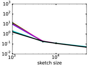
(a) $\|x-x^{\ast}\|_{2}/\|x^{\ast}\|_{2}$

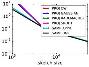
(b) $|f-f^{\ast}|/|f^{\ast}|$

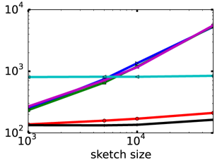
(c) Running time(sec)

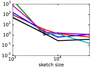
(d) $\|x-x^{\ast}\|_{2}/\|x^{\ast}\|_{2}$

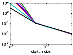
(e) $|f-f^{\ast}|/|f^{\ast}|$

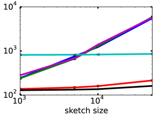
(f) Running time(sec)

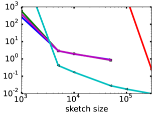
(g) $\|x-x^{\ast}\|_{2}/\|x^{\ast}\|_{2}$

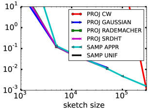
(h) $|f-f^{\ast}|/|f^{\ast}|$

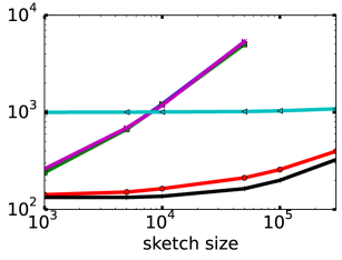
(i) Running time(sec)

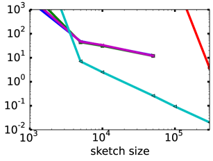
(j) $\|x-x^{\ast}\|_{2}/\|x^{\ast}\|_{2}$

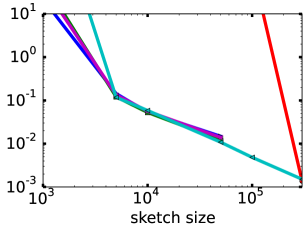
(k) $|f-f^{\ast}|/|f^{\ast}|$

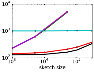
(l) Running time(sec)

Figure 3: Evaluation of all 6 of the algorithms on the 4 different types of matrices of size $1e7$ by $1000$. For each method, the following three quantities are computed: relative error of the objective $|f-f^{\ast}|/f^{\ast}$; relative error of the certificate $\|x-x^{\ast}\|_{2}/\|x^{\ast}\|_{2}$; and the running time to compute the approximate solution. Each subplot shows one of the above quantities versus the embedding dimension, respectively. For each setting, 3 independent trials are performed and the median is reported.

5.3.3 Quality of the approximate leverage scores

Here, we evaluate the quality of the fast approximate leverage score algorithm of [15], and we investigate the quality of the approximate leverage scores with several underlying embeddings. (The algorithm of [15] considered only Hadamard-based projections, but other projection methods could be used, leading to similar approximation quality but different running times.) We consider only an NB matrix since leverage scores with nonuniform distributions are harder to approximate. In addition, the size of the matrix we considered is only rather small, $1e6$ by $500$, due to the need to compute the exact leverage scores for comparison. Our implementation follows closely the main algorithm of [15], except that we consider other random projection matrices. In particular, we used the following four ways to compute the underlying embedding: namely, PROJ CW, PROJ GAUSSIAN, PROJ RADEMACHER, and PROJ SRDHT. For each kind of embedding and embedding dimension, we compute a series of quantities which characterize the statistical properties of the approximate leverage scores. The results are summarized in Table 12.

$c$	PROJ CW	PROJ GAUSSIAN	PROJ RADEMACHER	PROJ SRDH
	$\|\hat{p}-p^{\ast}\|_{2}/\|p^{\ast}\|_{2}$
5e2	0.9205	0.7738	0.7510	0.5008
1e3	0.9082	0.0617	0.0447	0.0716
5e3	0.9825	0.0204	0.0072	0.0117
1e4	0.9883	0.0143	0.0031	0.0075
5e4	0.9962	0.0061	0.0006	0.0030
1e5	0.0016	0.0046	0.0003	0.0023
	$D_{KL}(p^{\ast}||\hat{p})$
5e2	18.5241	0.0710	0.6372	0.1852
1e3	19.7773	0.0020	0.0015	0.0029
5e3	20.3450	0.0002	0.0001	0.0001
1e4	20.0017	0.0001	0.0001	0.0001
5e4	19.2417	1.9e-5	1.0e-5	1.0e-5
1e5	0.0001	1.0e-5	5e-6	5e-6
	$\alpha_{L}=\max_{i}\{\hat{p}^{L}_{i}/p_{i}^{\ast,L}\}$
5e2	28.6930	7.0267	7.3124	4.0005
1e3	11.4425	1.1596	1.1468	1.2201
5e3	50.3311	1.0584	1.0189	1.0379
1e4	82.6574	1.0449	1.0099	1.0199
5e4	218.9658	1.0192	1.0018	1.0094
1e5	1.0016	1.0108	1.0009	1.0060
	$\alpha_{S}=\max_{i}\{\hat{p}^{S}_{i}/p_{i}^{\ast,S}\}$
5e2	0	24.4511	16.8698	4.5227
1e3	0	1.3923	1.3718	1.3006
5e3	0	1.1078	1.1040	1.1077
1e4	0	1.0743	1.0691	1.0698
5e4	0	1.0332	1.0317	1.0310
1e5	1.0236	1.0220	1.0218	1.0198
	$\beta_{L}=\min_{i}\{\hat{p}^{L}_{i}/p_{i}^{\ast,L}\}$
5e2	0	0.0216	0.0448	0.4094
1e3	0	0.8473	0.8827	0.8906
5e3	0	0.9456	0.9825	0.9702
1e4	0	0.9539	0.9916	0.9827
5e4	0	0.9851	0.9982	0.9922
1e5	0.9969	0.9878	0.9993	0.9934
	$\beta_{S}=\min_{i}\{\hat{p}^{S}_{i}/p_{i}^{\ast,S}\}$
5e2	0	0.0077	0.0141	0.1884
1e3	0	0.7503	0.7551	0.7172
5e3	0	0.9037	0.9065	0.9065
1e4	0	0.9328	0.9306	0.9356
5e4	0	0.9704	0.9691	0.9710
1e5	0.9800	0.9787	0.9789	0.9803

Table 12: Quality of the approximate leverage scores. The test was performed on an NB matrix with size $1e6$ by $500$. In above, $\hat{p}$ denotes the distribution by normalizing the approximate leverage scores and $p^{\ast}$ denotes the exact leverage score distribution. $D_{KL}(p||q)$ is the KL divergence [86] of $q$ from $p$ defined as $\sum_{i}p_{i}\ln\frac{p_{i}}{q_{i}}$. Let $L=\{i|p^{\ast}_{i}=1\}$ and $S=\{i|p^{\ast}_{i}<1\}$. In this case, $\hat{p}^{L}$ denotes the corresponding slice of $\hat{p}$, and the quantities $\hat{p}^{S},p^{\ast,L},p^{\ast.S}$ are defined similarly.

As we can see, when the projection size is large enough, all the projection-based methods to compute approximations to the leverage scores produce highly accurate leverage scores. Among these projection methods, PROJ CW is typically faster but also requires a much larger projection size in order to yield reliable approximate leverage scores. The other three random projections perform similarly. In general, the algorithms approximate the large leverage scores (those that equal or are close to $1$) better than the small leverage scores, since $\alpha_{L}$ and $\beta_{L}$ are closer to $1$. This is crucial when calling SAMP APPR since the important rows shall not be missed, and it is a sufficient condition for the theory underlying the algorithm of [15] to apply.

Next, we invoke the sampling algorithm for the $\ell_{2}$ regression problem, with sampling size $s=1e4$ by using these approximate leverage scores. We evaluate the relative error on both the solution vector and objective and the total running time. For completeness and in order to evaluate the quality of the approximate leverage score algorithm, we also include the results by using the exact leverage scores. The results are presented in Figure 4.

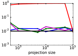
(a) $\|x-x^{\ast}\|_{2}/\|x^{\ast}\|_{2}$

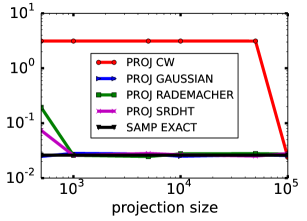
(b) $|f-f^{\ast}|/|f^{\ast}|$

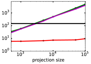
(c) Running time(sec)

Figure 4: Performance of sampling algorithms with approximate leverage scores, as computed by several different underlying projections. The test was performed on an NB matrix of size $1e6$ by $500$ and the sampling size was $1e4$. Each subplot shows one of the following three quantities versus the projection size used in the underlying random projection phase: relative error of the objective $|f-f^{\ast}|/f^{\ast}$; relative error of the certificate $\|x-x^{\ast}\|_{2}/\|x^{\ast}\|_{2}$; and the running time. For each setting, 5 independent trials are performed and the median is reported.

These results suggest that the precise quality of the approximate leverage scores does not substantially affect the downstream error, i.e., sampling-based algorithms are robust to imperfectly-approximated leverage scores, as long as the largest scores are not too poorly approximated. (Clearly, however, we could have chosen parameters such that some of the larger scores were very poorly approximated, e.g., by choosing the embedding dimension to be too small, in which case the quality would matter. In our experience, the quality matters less since these approximate leverage scores are sufficient to solve $\ell_{2}$ regression problems.) Finally, and importantly, note that the solution quality obtained by using approximate leverage scores is as good as that of using exact leverage scores, while the running time can be much less.

5.3.4 Performance of low-precision solvers when $n$ changes

Here, we explore the scalability of the low-precision solvers by evaluating the performance of all the embeddings on NB matrices with varying $n$. We fix $d=1000$ and let $n$ take values from $2.5e5$ to $1e8$. These matrices are generated by stacking an NB matrix with size $2.5e5$ by $1000$ REPNUM times, with REPNUM varying from $1$ to $400$ using STACK1. For conciseness, we fix the embedding dimension of each method to be either $5e3$ or $5e4$. The relative error on certificate and objective and running time are evaluated. The results are presented in Figure 5.

Especially worthy mentioning is that when using STACK1, by increasing REPNUM, as we pointed out, the coherence of the matrix, i.e., the maximum leverage score, is decreasing, as the size is increased. We can clearly see that, when $n=2.5e5$, i.e., the coherence is $1$, PROJ CW fails. Once the coherence gets smaller, i.e., $n$ gets larger, the projection-based methods behave similarly and the relative error remains roughly the same as we increased $n$. This is because STACK1 doesn’t alter the condition number and the amount of mass of the right hand side vector that lies in the range space of the design matrix and the lower dimension $d$ remains the same. However, SAMP APPR tends to yield larger error on approximating the certificate as we increase REPNUM, i.e., the coherence gets smaller. Moreover, it breaks down when the embedding dimension is very small.

$s=5e3$
$s=5e4$

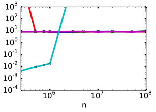
(a) $\|x-x^{\ast}\|_{2}/\|x^{\ast}\|_{2}$

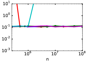
(b) $|f-f^{\ast}|/|f^{\ast}|$

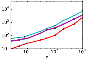
(c) Running time(sec)

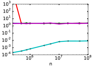
(d) $\|x-x^{\ast}\|_{2}/\|x^{\ast}\|_{2}$

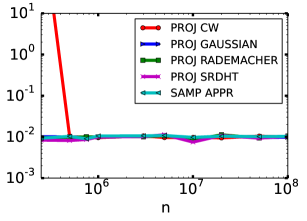
(e) $|f-f^{\ast}|/|f^{\ast}|$

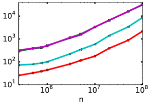
(f) Running time(sec)

Figure 5: Performance of all the algorithms on NB matrices with varying $n$ from $2.5e5$ to $1e8$ and fixed $d=1000$. The matrix is generated using STACK1. For each method, the embedding dimension is fixed to be $5e3$ or $5e4$. The following three quantities are computed: relative error of the objective $|f-f^{\ast}|/f^{\ast}$; relative error of the certificate $\|x-x^{\ast}\|_{2}/\|x^{\ast}\|_{2}$; and the running time to compute the approximate solution. For each setting, 3 independent trials are performed and the median is reported.

5.3.5 Performance of low-precision solvers when $d$ changes

Here, we evaluate the performance of the low-precision solvers by evaluating the performance of all the embeddings on NB matrices with changing $d$. We fix $n=1e7$ and let $d$ take values from $10$ to $2000$. For each $d$, the matrix is generated by stacking an NB matrix with size $2.5e5$ by $d$ 40 times using STACK1, so that the coherence of the matrix is $1/40$. For conciseness, we fix the embedding of each method to be $2e3$ or $5e4$. The relative error on certificate and objective and running time are evaluated. The results are shown in Figure 6.

As can be seen, overall, all the projection-based methods behave similarly. As expected, the relative error goes up as $d$ gets larger. Meanwhile, SAMP APPR yields lower error as $d$ increases. However, it seems to have a stronger dependence on the lower dimension of the matrix, as it breaks down when $d$ is $100$ for small sampling size, i.e., $s=2e3$.

$s=2e3$
$s=5e4$

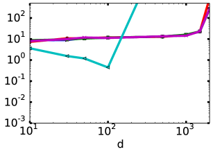
(a) $\|x-x^{\ast}\|_{2}/\|x^{\ast}\|_{2}$

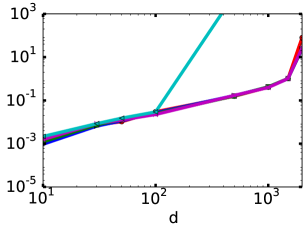
(b) $|f-f^{\ast}|/|f^{\ast}|$

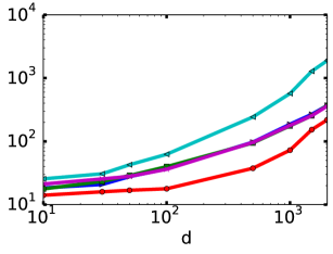
(c) Running time(sec)

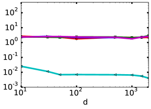
(d) $\|x-x^{\ast}\|_{2}/\|x^{\ast}\|_{2}$

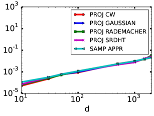
(e) $|f-f^{\ast}|/|f^{\ast}|$

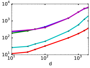
(f) Running time(sec)

Figure 6: Performance of all the algorithms on NB matrices with varying $d$ from $10$ to $2000$ and fixed $n=1e7$. The matrix is generated using STACK1. For each method, the embedding dimension is fixed to be $2e3$ or $5e4$. The following three quantities are computed: relative error of the objective $|f-f^{\ast}|/f^{\ast}$; relative error of the certificate $\|x-x^{\ast}\|_{2}/\|x^{\ast}\|_{2}$; and the running time to compute the approximate solution. For each setting, 3 independent trials are performed and the median is reported.

5.3.6 Performance of high precision solvers

Here, we evaluate the use of these methods as preconditioners for high-precision iterative solvers. Since the embedding can be used to compute a preconditioner for the original linear system, one can invoke iterative algorithms such as LSQR [43] to solve the preconditioned least-squares problem. Here, we will use LSQR. We first evaluate the conditioning quality, i.e., $\kappa(AR^{-1})$, on an NB matrix with size $1e6$ by $500$ using several different ways for computing the embedding. The results are presented in Table 13. Then we test the performance of LSQR with these preconditioners on an NB matrix with size $1e8$ by $1000$ and an NG matrix with size $1e7$ by $1000$. For simplicity, for each method of computing the embedding, we try a small embedding dimension where some of the methods fail, and a large embedding dimension where most of the methods succeed. See Figure 7 and Figure 8 for details.

The convergence rate of the LSQR phase depends on the preconditioning quality, i.e., $\kappa(AR^{-1})$ where $R$ is obtained by the QR decomposition of the embedding of $A$, $\Phi A$. See Section 4.2 for more details. Table 13 implies that all the projection-based methods tend to yield preconditioners with similar condition numbers once the embedding dimension is large enough. Among them, PROJ CW needs a much larger embedding dimension to be reliable (clearly consistent with its use in low-precision solvers). In addition, overall, the conditioning quality of the sampling-based embedding method, i.e., SAMP APPR tends to be worse than that of projection-based methods.

As for the downstream performance, from Figure 7 we can clearly see that, when a small embedding dimension is used, i.e., $s=5e3$, PROJ GAUSSIAN yields the best preconditioner, as its better preconditioning quality translates immediately into fewer iterations for LSQR to converge. This is followed by SAMP APPR. This relative order is also suggested by Table 13. As the embedding dimension is increased, i.e., using large embedding dimension, all the method yield significant improvements and produce much more accurate solutions compared to that of NOCO (LSQR without preconditioning), among which PROJ CW with embedding dimension $3e5$ converges to a nearly machine-precision solution within only $5$ iterations. As for the running time, since each iteration of LSQR only involves with two matrix-vector multiplications (costs less than 2 minutes in our experiments), the overall running time is dominated by the time for computing the preconditioner. As expected, PROJ CW runs the fastest and the running time of PROJ GAUSSIAN scales linearly in the embedding dimension. In SAMP APPR, the sampling process needs to make $1$-$2$ passes over the dataset but the running time is relatively stable regardless of the sampling size, as reflected in Figure 7(c)&(f). Finally, note that the reason that the error does not drop monotonically in the solution vector is the following. With the preconditioners, we work on a transformed system, and the theory only guarantees monotonicity in the decreasing of the relative error of the certificate of the transformed system, not the original one.

Finally, a minor but potentially important point should be mentioned as a word of caution. As expected, when the condition number of the linear system is large, vanilla LSQR does not converge at all. On the other hand, when the condition number is very small, from Figure 8, there is no need to precondition. If, in this latter case, a randomized preconditioning method is used, then the embedding dimension must be chosen to be sufficiently large: unless the embedding dimension is large enough such that the conditioning quality is sufficiently good, then preconditioned LSQR yields larger errors than even vanilla LSQR.

$c$	PROJ CW	PROJ GAUSSIAN	PROJ RADEMACHER	PROJ SRDHT	SAMP APPR
5e2	1.08e8	2.17e3	1.42e3	1.19e2	1.21e2
1e3	1.1e6	5.7366	5.6006	7.1958	75.0290
5e3	5.5e5	1.9059	1.9017	1.9857	25.8725
1e4	5.1e5	1.5733	1.5656	1.6167	17.0679
5e4	1.8e5	1.2214	1.2197	1.2293	6.9109
1e5	1.1376	1.1505	1.1502	1.1502	4.7573

Table 13: Quality of preconditioning on an NB matrix with size $1e6$ by $500$ using several kinds of embeddings. For each setting, 5 independent trials are performed and the median is reported.

small embedding dimension
large embedding dimension

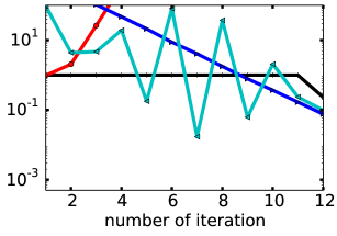
(a) $\|x-x^{\ast}\|_{2}/\|x^{\ast}\|_{2}$

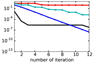
(b) $|f-f^{\ast}|/|f^{\ast}|$

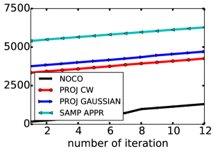
(c) Running time(sec)

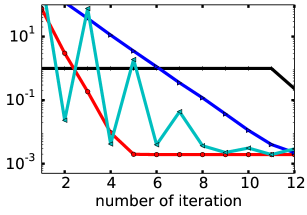
(d) $\|x-x^{\ast}\|_{2}/\|x^{\ast}\|_{2}$

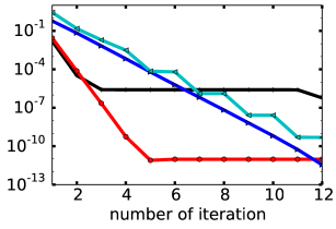
(e) $|f-f^{\ast}|/|f^{\ast}|$

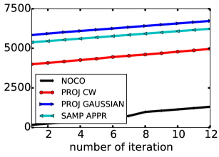
(f) Running time(sec)

Figure 7: Evaluation of LSQR with randomized preconditioner on an NB matrix with size $1e8$ by $1000$ and condition number $1e6$. Here, several ways for computing the embedding are implemented. In SAMP APPR, the underlying random projection is PROJ CW with projection dimension $3e5$. For completeness, LSQR without preconditioner is evaluated, denoted by NOCO. In above, by small embedding dimension, we mean $5e3$ for all the methods. By large embedding dimension, we mean 3e5 for PROJ CW, 1e4 for PROJ GAUSSIAN and 5e4 for SAMP APPR. For each method and embedding dimension, the following three quantities are computed: relative error of the objective $|f-f^{\ast}|/f^{\ast}$; relative error of the certificate $\|x-x^{\ast}\|_{2}/\|x^{\ast}\|_{2}$; and the running time to compute the approximate solution. Each subplot shows one of the above quantities versus number of iteration, respectively. For each setting, only one trial is performed.

small embedding dimension
large embedding dimension

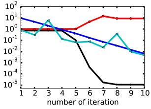
(a) $\|x-x^{\ast}\|_{2}/\|x^{\ast}\|_{2}$

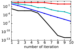
(b) $|f-f^{\ast}|/|f^{\ast}|$

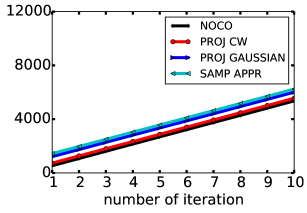
(c) Running time(sec)

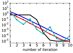
(d) $\|x-x^{\ast}\|_{2}/\|x^{\ast}\|_{2}$

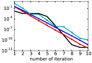
(e) $|f-f^{\ast}|/|f^{\ast}|$

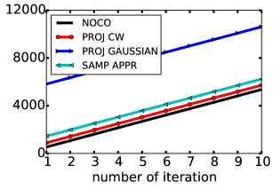
(f) Running time(sec)

Figure 8: Evaluation of LSQR with randomized preconditioner on an NB matrix with size $1e7$ by $1000$ and condition number $5$. Here, several ways for computing the embedding are implemented. In SAMP APPR, the underlying random projection is PROJ CW with projection dimension $3e5$. For completeness, LSQR without preconditioner is evaluated, denoted by NOCO. In above, by small embedding dimension, we mean $5e3$ for all the methods. By large embedding dimension, we mean $3e5$ for PROJ CW and $5e4$ for the rest. For each method and embedding dimension, the following three quantities are computed: relative error of the objective $|f-f^{\ast}|/f^{\ast}$; relative error of the certificate $\|x-x^{\ast}\|_{2}/\|x^{\ast}\|_{2}$; and the running time to compute the approximate solution. Each subplot shows one of the above quantities versus number of iteration, respectively. For each setting, 3 independent trials are performed and the median is reported.

6 Discussion and conclusion

Large-scale data analysis and machine learning problems present considerable challenges and opportunities to signal processing, electrical engineering, scientific computing, numerical linear algebra, and other research areas that have historically been developers of and/or consumers of high-quality matrix algorithms. RandNLA is an approach, originally from theoretical computer science, that uses randomization as a resource for the development of improved matrix algorithms, and it has had several remarkable successes in theory and in practice in small to medium scale matrix computations in RAM. The general design strategy of RandNLA algorithms (for problems such as $\ell_{2}$ regression and low-rank matrix approximation) in RAM is by now well known: construct a sketch (either by performing a random projection or by random sampling according to a judiciously-chosen data-dependent importance sampling probability distribution), and then use that sketch to approximate the solution to the original problem (either by solving a subproblem on the sketch or using the sketch to construct a preconditioner for the original problem).

The work reviewed here highlights how, with appropriate modifications, similar design strategies can extend (for $\ell_{2}$-based regression problems as well as other problems such as $\ell_{1}$-based regression problems) to much larger-scale parallel and distributed environments that are increasingly common. Importantly, though, the improved scalability often comes due to restricted communications, rather than improvements in FLOPS. (For example, the use of Chebyshev semi-iterative method vs. LSQR in LSRN on MPI; and the use of the MIE with multiple queries on MapReduce.) In these parallel/distributed settings, we can take advantage of the communication-avoiding nature of RandNLA algorithms to move beyond FLOPS to design matrix algorithms that use more computation than the traditional algorithms but that have much better communication profiles, and we can do this by mapping the RandNLA algorithms to the underlying architecture in very nontrivial ways. (For example, using more computationally-expensive Gaussian projections to ensure stronger control on the condition number; and using the MIE with multiple initial queries to construct a very good initial search region.) These examples of performing extra computation to develop algorithms with improved communication suggests revisiting other methods from numerical linear algebra, optimization, and scientific computing, looking in other novel ways beyond FLOPS for better communication properties for many large-scale matrix algorithms.

Acknowledgments. We would like to thank Michael Saunders for advice and helpful discussions. We would also like to acknowledge the Army Research Office, the Defense Advanced Research Projects Agency, and the Department of Energy for providing partial support for this work.

References

- [1] M. W. Mahoney. Randomized Algorithms for Matrices and Data. Foundations and Trends in Machine Learning. NOW Publishers, Boston, 2011. Also available at arXiv:1104.5557v2.
- [2] A. Torralba, R. Fergus, and W. T. Freeman. 80 million tiny images: A large data set for nonparametric object and scene recognition. IEEE Trans. Pattern Anal. Mach. Intell., 30(11):1958–1970, 2008.
- [3] G. Werner-Allen, J. Johnson, M. Ruiz, J. Lees, and M. Welsh. Monitoring volcanic eruptions with a wireless sensor network. In Proceeedings of the 2nd European Workshop on Wireless Sensor Networks, pages 108–120. IEEE, 2005.
- [4] J. Dean and S. Ghemawat. MapReduce: Simplified data processing on large clusters. In Proceedings of the 6th Symposium on Operating System Design and Implementation (OSDI), pages 137–149, 2004.
- [5] L. G. Valiant. A bridging model for parallel computation. Communications of the ACM, 33(8):103–111, 1990.
- [6] A. Aggarwal, A. K. Chandra, and M. Snir. Communication complexity of PRAMs. Theoretical Computer Science, 71(1):3–28, 1990.
- [7] B. Lint and T. Agerwala. Communication issues in the design and analysis of parallel algorithms. IEEE Transactions on Software Engineering, SE-7(2):174–188, 1981.
- [8] D. Heller. A survey of parallel algorithms in numerical linear algebra. SIAM Review, 20(4):740–777, 1976.
- [9] S. Toledo. A survey of out-of-core algorithms in numerical linear algebra. In J. M. Abello and J. S. Vitter, editors, External memory algorithms, Dimacs Series In Discrete Mathematics And Theoretical Computer Science, pages 161–179. American Mathematical Society, 1999.
- [10] G. Ballard, J. Demmel, O. Holtz, and O. Schwartz. Minimizing communication in numerical linear algebra. SIAM Journal on Matrix Analysis and Applications, 32(3):866–901, 2011.
- [11] D. P. Bertsekas and J. N. Tsitsiklis. Some aspects of parallel and distributed iterative algorithms—a survey. Automatica, 27(1):3–21, 1991.
- [12] N. Halko, P. G. Martinsson, and J. A. Tropp. Finding structure with randomness: Probabilistic algorithms for constructing approximate matrix decompositions. SIAM Review, 53(2):217–288, 2011.
- [13] D. P. Woodruff. Sketching as a Tool for Numerical Linear Algebra. Foundations and Trends in Theoretical Computer Science. NOW Publishers, Boston, 2014.
- [14] P. Drineas, M. W. Mahoney, and S. Muthukrishnan. Sampling algorithms for regression and applications. In Proceedings of the 17th Annual ACM-SIAM Symposium on Discrete Algorithms (SODA), pages 1127–1136. ACM, 2006.
- [15] P. Drineas, M. Magdon-Ismail, M. W. Mahoney, and D. P. Woodruff. Fast approximation of matrix coherence and statistical leverage. Journal of Machine Learning Research, 13:3475–3506, 2012.
- [16] P. Ma, M. W. Mahoney, and B. Yu. A statistical perspective on algorithmic leveraging. Journal of Machine Learning Research.
- [17] P. Drineas, M .W. Mahoney, and S. Muthukrishnan. Relative-error CUR matrix decompositions. SIAM Journal on Matrix Analysis and Applications, 30:844–881, 2008.
- [18] M. W. Mahoney and P. Drineas. CUR matrix decompositions for improved data analysis. Proc. Natl. Acad. Sci. USA, 106:697–702, 2009.
- [19] K. L. Clarkson, P. Drineas, M. Magdon-Ismail, M. W. Mahoney, X. Meng, and D. P. Woodruff. The Fast Cauchy Transform and faster robust linear regression. In Proceedings of the 24th Annual ACM-SIAM Symposium on Discrete Algorithms (SODA), 2013.
- [20] K. L. Clarkson and D. P. Woodruff. Low rank approximation and regression in input sparsity time. In Proceedings of the 45th Annual ACM symposium on Theory of Computing (STOC), 2013.
- [21] A. Gittens and M. W. Mahoney. Revisiting the Nyström method for improved large-scale machine learning. Technical report, 2013. Preprint: arXiv:1303.1849.
- [22] E. J. Candes and B. Recht. Exact matrix completion via convex optimization. Communications of the ACM, 55(6):111–119, 2012.
- [23] D. C. Hoaglin and R. E. Welsch. The hat matrix in regression and ANOVA. The American Statistician, 32(1):17–22, 1978.
- [24] S. Chatterjee and A. S. Hadi. Influential observations, high leverage points, and outliers in linear regression. Statistical Science, 1(3):379–393, 1986.
- [25] P. F. Velleman and R. E. Welsch. Efficient computing of regression diagnostics. The American Statistician, 35(4):234–242, 1981.
- [26] S. Chatterjee and A.S. Hadi. Sensitivity Analysis in Linear Regression. John Wiley & Sons, New York, 1988.
- [27] R. Motwani and P. Raghavan. Randomized Algorithms. Cambridge University Press, New York, 1995.
- [28] T. Sarlós. Improved approximation algorithms for large matrices via random projections. In Proceedings of the 47th Annual IEEE Symposium on Foundations of Computer Science (FOCS), pages 143–152. IEEE, 2006.
- [29] P. Drineas, M. W. Mahoney, S. Muthukrishnan, and T. Sarlós. Faster least squares approximation. Numer. Math., 117(2):219–249, 2011.
- [30] V. Rokhlin and M. Tygert. A fast randomized algorithm for overdetermined linear least-squares regression. Proc. Natl. Acad. Sci. USA, 105(36):13212–13217, 2008.
- [31] H. Avron, P. Maymounkov, and S. Toledo. Blendenpik: Supercharging LAPACK’s least-squares solver. SIAM J. Sci. Comput., 32(3):1217–1236, 2010.
- [32] X. Meng, M. A. Saunders, and M. W. Mahoney. LSRN: A parallel iterative solver for strongly over- or under-determined systems. SIAM J. Sci. Comput., 36(2):95–118, 2014.
- [33] E. S. Coakley, V. Rokhlin, and M. Tygert. A fast randomized algorithm for orthogonal projection. SIAM J. Sci. Comput., 33(2):849–868, 2011.
- [34] Y. Nesterov. Unconstrained convex minimization in relative scale. Mathematics of Operations Research, 34(1):180–193, 2009.
- [35] A. Dasgupta, P. Drineas, B. Harb, R. Kumar, and M. W. Mahoney. Sampling algorithms and coresets for regression. SIAM J. Comput., 38(5):2060–2078, 2009.
- [36] F. John. Extremum problems with inequalities as subsidiary conditions. In Studies and Essays presented to R. Courant on his 60th Birthday, pages 187–204, 1948.
- [37] Å. Björck. Numerical Methods for Least Squares Problems. SIAM, 1996.
- [38] G. H. Golub and C. F. Van Loan. Matrix Computations. Johns Hopkins Univ Press, third edition, 1996.
- [39] Å. Björck. Stability analysis of the method of seminormal equations for linear least squares problems. Linear Algebra and its Applications, 88:31–48.
- [40] T. A. Davis. Direct Methods for Sparse Linear Systems. SIAM, Philadelphia, 2006.
- [41] C. C. Paige and M. A. Saunders. Solution of sparse indefinite systems of linear equations. SIAM J. Numer. Anal., 12(4):617–629, 1975.
- [42] M. R. Hestenes and E. Stiefel. Methods of conjugate gradients for solving linear systems. J. Res. Nat. Bur. Stand., 49(6):409–436, 1952.
- [43] C. C. Paige and M. A. Saunders. LSQR: An algorithm for sparse linear equations and sparse least squares. ACM Trans. Math. Softw., 8(1):43–71, 1982.
- [44] D. C.-L. Fong and M. Saunders. LSMR: An iterative algorithm for sparse least-squares problems. SIAM J. Sci. Comput., 33:2950, 2011.
- [45] G. H. Golub and R. S. Varga. Chebyshev semi-iterative methods, successive over-relaxation methods, and second-order Richardson iterative methods, parts I and II. Numer. Math., 3(1):147–168, 1961.
- [46] D. G. Luenberger. Introduction to Linear and Nonlinear Programming. Addison-Wesley, 1973.
- [47] Y. Nesterov. Introductory Lectures on Convex Optimization: A Basic Course, volume 87. Springer, 2004.
- [48] Y. Ye. Interior Point Algorithms: Theory and Analysis, volume 44. John Wiley & Sons, 2011.
- [49] J. E. Mitchell. Polynomial interior point cutting plane methods. Optimization Methods and Software, 18(5):507–534, 2003.
- [50] S. Boyd and L. Vandenberghe. Convex Optimization. Cambridge University Press, 2004.
- [51] K. L. Clarkson. Subgradient and sampling algorithms for regression. In Proceedings of the 16th Annual ACM-SIAM Symposium on Discrete Algorithms (SODA), pages 257–266. SIAM, 2005.
- [52] Y. Nesterov. Smooth minimization of non-smooth functions. Mathematical Programming, 103(1):127–152, 2005.
- [53] G. B. Dantzig. Linear Programming and Extensions. Princeton University Press, 1998.
- [54] Y. Nesterov. Rounding of convex sets and efficient gradient methods for linear programming problems. Optimization Methods and Software, 23(1):109–128, 2008.
- [55] S. A. Vavasis and Y. Ye. Condition numbers for polyhedra with real number data. Operations Research Letters, 17(5):209–214, 1995.
- [56] P. W. Holland and R. E. Welsch. Robust regression using iteratively reweighted least-squares. Communications in Statistics - Theory and Methods, 6(9):813–827, 1977.
- [57] C. S. Burrus. Iterative reweighted least squares, 12 2012. http://cnx.org/content/m45285/1.12/.
- [58] G. Barequet and S. Har-Peled. Efficiently approximating the minimum-volume bounding box of a point set in three dimensions. Journal of Algorithms, 38(1):91–109, 2001.
- [59] L. Lovász. An Algorithmic Theory of Numbers, Graphs, and Convexity. SIAM, 1986.
- [60] C. Bouville. Bounding ellipsoids for ray-fractal intersection. In ACM SIGGRAPH Computer Graphics, volume 19, pages 45–52. ACM, 1985.
- [61] L. G. Khachiyan and M. J. Todd. On the complexity of approximating the maximal inscribed ellipsoid for a polytope. Math. Prog., 61(1):137–159, 1993.
- [62] X. Meng and M. W. Mahoney. Robust regression on MapReduce. In Proceedings of the 30th International Conference on Machine Learning (ICML), 2013.
- [63] C. Sohler and D. P. Woodruff. Subspace embeddings for the -norm with applications. In Proceedings of the 43rd Annual ACM Symposium on Theory of Computing (STOC), pages 755–764. ACM, 2011.
- [64] David P. Woodruff and Qin Zhang. Subspace embeddings and -regression using exponential random variables. In COLT, volume 30, pages 546–567, 2013.
- [65] J. A. Tropp. Improved analysis of the subsampled randomized Hadamard transform. Adv. Adapt. Data Anal., 3(1-2):115–126, 2011.
- [66] X. Meng and M. W. Mahoney. Low-distortion subspace embeddings in input-sparsity time and applications to robust linear regression. In Proceedings of the 45th Annual ACM Symposium on Theory of Computing (STOC), 2013.
- [67] J. Nelson and H. Nguyen. OSNAP: Faster numerical linear algebra algorithms via sparser subspace embeddings. In Proceedings of the 54th Annual IEEE Symposium on Foundations of Computer Science (FOCS), pages 117–126. IEEE, 2013.
- [68] W. B. Johnson and J. Lindenstrauss. Extensions of Lipschitz mappings into a Hilbert space. Contemporary Mathematics, 26(189-206):1, 1984.
- [69] P. Indyk and R. Motwani. Approximate nearest neighbors: towards removing the curse of dimensionality. In Proceedings of the 30th Annual ACM Symposium on Theory of Computing (STOC), pages 604–613. ACM, 1998.
- [70] D. Achlioptas. Database-friendly random projections. In Proceedings of the 20th ACM SIGMOD-SIGACT-SIGART Symposium on Principles of Database Systems (PODS), pages 274–281. ACM, 2001.
- [71] K. R. Davidson and S. J. Szarek. Local operator theory, random matrices and Banach spaces. In Handbook of the Geometry of Banach Spaces, volume 1, pages 317–366. North Holland, 2001.
- [72] N. Ailon and B. Chazelle. Approximate nearest neighbors and the fast Johnson-Lindenstrauss transform. In Proceedings of the 38th Annual ACM Symposium on Theory of Computing (STOC), pages 557–563. ACM, 2006.
- [73] N. Ailon and B. Chazelle. The fast Johnson-Lindenstrauss transform and approximate nearest neighbors. SIAM J. Comput., 39(1):302–322, 2009.
- [74] N. Ailon and E. Liberty. Fast dimension reduction using Rademacher series on dual BCH codes. Discrete & Computational Geometry, 42(4):615–630, 2009.
- [75] N. Ailon and E. Liberty. An almost optimal unrestricted fast Johnson-Lindenstrauss transform. In Proceedings of the 22nd Annual ACM-SIAM Symposium on Discrete Algorithms (SODA), pages 185–191, 2011.
- [76] M. Charikar, K. Chen, and M. Farach-Colton. Finding frequent items in data streams. In Automata, Languages and Programming, pages 693–703. Springer, 2002.
- [77] J. Yang, X. Meng, and M. W. Mahoney. Quantile regression for large-scale applications. SIAM J. Sci. Comput., 36(5):S78–S110, 2014.
- [78] M. Charikar and A. Sahai. Dimension reduction in the norm. In Proceedings of the 43rd Annual IEEE Symposium on Foundations of Computer Science (FOCS), pages 551–560, 2002.
- [79] Y. Nesterov and A. Nemirovsky. Interior Point Polynomial Methods in Convex Programming. SIAM, 1994.
- [80] S. Portnoy and R. Koenker. The Gaussian hare and the Laplacian tortoise: computability of squared-error versus absolute-error estimators. Statistical Science, 12(4):279–300, 1997.
- [81] S. Portnoy. On computation of regression quantiles: Making the Laplacian tortoise faster. Lecture Notes-Monograph Series, Vol. 31, -Statistical Procedures and Related Topics, pages 187–200, 1997.
- [82] G. Marsaglia and W. W. Tsang. The ziggurat method for generating random variables. J. Stat. Softw., 5(8):1–7, 2000.
- [83] M. Grötschel, L. Lovász, and A. Schrijver. The ellipsoid method and its consequences in combinatorial optimization. Combinatorica, 1(2):169–197, 1981.
- [84] S. Tarasov, L. G. Khachiyan, and I. Erlikh. The method of inscribed ellipsoids. In Soviet Mathematics Doklady, volume 37, pages 226–230, 1988.
- [85] R. N. Bracewell. Discrete hartley transform. J. Opt. Soc. Am., 73(12):1832–1835, 1983.
- [86] S. Kullback and R. A. Leibler. On information and sufficiency. Ann. Math. Statist., 22(1):79–86, 1951.