Angular asymmetries as a probe
for anomalous contributions to $HZZ$ vertex at the LHC

Abstract

In this article, the prospects for studying the tensor structure of the $HZZ$ vertex with the LHC experiments are presented. The structure of tensor couplings in Higgs di-boson decays is investigated by measuring the asymmetries and by studing the shapes of the final state angular distributions. The expected background contributions, detector resolution, and trigger and selection efficiencies are taken into account. The potential of the LHC experiments to discover sizeable non-Standard Model contributions to the $HZZ$ vertex with $300\;{\rm fb}^{-1}$ and $3000\;{\rm fb}^{-1}$ is demonstrated.

I Introduction

In the Summer of 2012, the CMS and ATLAS Collaborations at the LHC reported the discovery of a new neutral resonance in searches for the Standard Model Higgs boson. This discovery was later confirmed by analyses of the full LHC Run-I dataset by both collaborations cms_higgs ; atlas_higgs . It was demonstrated that the new particle with a mass around $125.5$ GeV was dominantly produced via the gluon-fusion process and decays into pairs of gauge bosons: $\gamma\gamma$, $ZZ$ and $WW$. The observed production and decay modes identified the discovered particle as a neutral boson. The subsequent measurement of its couplings to fermions and bosons demonstrated the compatibility of the discovered resonance with the expectations for the Standard Model Higgs boson within available statistics atlas_couplings ; Khachatryan:2014kca ; Chatrchyan:2012jja .

In the Standard Model, electroweak symmetry breaking via the Higgs mechanism requires the presence of a single neutral Higgs boson with spin 0 and even CP-parity. Theories beyond the Standard Model often require an extended Higgs sector featuring several neutral Higgs bosons of both even and odd CP-parity. In such a case, mixing between Higgs boson CP-eigenstates is possible. The Higgs boson mass eigenstates observed in experiment may thus have mixed CP-parity. Such an extension of the Higgs sector is important because effects of CP violation in the SM are too small and, in particular, cannot explain the baryon asymmetry of the Universe.

Dedicated studies of spin and parity of the Higgs candidate discovered by ATLAS and CMS showed that its dominant spin and parity are compatible with $J^{CP}=0^{++}$ atlas_spin ; Chatrchyan:2012jja ; Khachatryan:2014kca . The dataset of about $25\;{\rm fb}^{-1}$ currently collected by each of the major LHC experiments allows to set an upper limit on the possible CP-odd contribution. The sensitivity is expected to improve with larger datasets to be collected at the LHC.

There have been many works on direct measurement of CP violation in the Higgs sector  Chang:1993jy ; Grzadkowski:1995rx ; Gunion:1996vv ; Grzadkowski:1999ye ; Grzadkowski:2000hm ; Plehn:2001nj ; Choi:2002jk ; Buszello:2002uu ; Hankele:2006ma ; Godbole:2007cn ; Keung:2008ve ; Berge:2008dr ; Cao:2009ah ; DeRujula:2010ys ; Gao:2010qx ; Berge:2011ij ; Bishara:2013vya ; Harnik:2013aja ; Berge:2013jra ; Modak:2013sb ; Chen:2014gka ; Gainer:2013rxa ; Avery:2012um ; Gainer:2014hha ; Chen:2013waa ; Stolarski:2012ps . In this paper the sensitivity of LHC experiments to observe CP-mixing effects with $300\;{\rm fb}^{-1}$ and $3000\;{\rm fb}^{-1}$ is evaluated using the method of angular asymmetries.

This paper is organised as follows. In Section II observables sensitive to CP violation in the $HZZ$ vertex are discussed. The spin-0 model, a Monte Carlo production of signal and background, and a lagrangian parametrisation for CP-mixing measurements are discussed in Section III. In Section IV the expected sensitivity of the LHC experiments to the CP-violation effects based on angular asymmetries is presented. Constraits are set on the contribution of anomalous couplings to the $HZZ$ vertex. Section V introduces the measurement technique based on observables fit. Exclusion regions for the mixing angle are presented. Section VI gives the overall summary of obtained results.

II Observables

In this paper we study the sensitivity of final state observables to the CP violating $HZZ$ vertex in the process:

$$gg\to H\to ZZ\to 4l.$$ (1)

Following the notation introduced in Gao:2010qx , the general scattering amplitude describing interactions of a spin-zero boson with the gauge bosons is given by:

$$A(X\to VV)=\frac{1}{v}\big{(}g_{1}m_{V}^{2}\epsilon_{1}^{\ast}\epsilon_{2}^{\ast}+g_{2}f_{\mu\nu}^{\ast(1)}f^{\ast(2)\mu\nu}$$

$$+\;g_{4}f^{\ast(1)}_{\mu\nu}{\tilde{f}}^{\ast(2)\mu\nu}\big{)}\,.$$ (2)

Here the $f^{(i){\mu\nu}}=\epsilon_{i}^{\mu}q_{i}^{\nu}-\epsilon_{i}^{\nu}q_{i}^{\mu}$ is the field strength tensor of a gauge boson with momentum $q_{i}$ and polarisation vector $\epsilon_{i}$; ${\tilde{f}}^{(i)\mu\nu}=1/2\epsilon^{\mu\nu\alpha\beta}f_{\alpha\beta}$ is the conjugate field strength tensor. The symbols $v$ and $m_{V}$ denote the SM vacuum expectation value of the Higgs field and the mass of the gauge boson respectively.

In the Standard Model, the only non-vanishing coupling of the Higgs to $ZZ$ or $WW$ boson pairs at tree-level is $g_{1}=2i$, while $g_{2}$ is generated through radiative corrections. For final states with at least one massless gauge boson, such as $\gamma\gamma$, $gg$ or $Z\gamma$, the SM interactions with the Higgs boson are loop-induced. These interactions are described by the coupling $g_{2}$. The coupling $g_{4}$ is associated with the interaction of CP-odd Higgs boson with a pair of gauge bosons. The simultaneous presence of CP-even terms $g_{1}$ and/or $g_{2}$ and the CP-odd term $g_{4}$ leads to CP violation.

In general, $g_{i}$ couplings can be complex and momentum dependent. However imaginary parts of these couplings are generated by absorptive parts of the corresponding diagrams and expected to be small: approximately less than $1\%$. We further assume that the energy scale of new physics is around $1$ TeV or higher, so that the momentum dependence of the couplings can be neglected. Thus, in the following we will consider $g_{i}$ couplings as real and momentum-independent.

These assumptions are entirely consistent with the framework of an effective field theory (EFT) of the SM. If the energy scale of the new physics is much higher than the electroweak scale new effects can be described by an EFT with the SM Lagrangian supplemented by higher dimension operators of $d=6$. Such an approach was worked out in detail in Buchmuller:1985jz ; Grzadkowski:2010es

One of possibilities to study CP violation in the process of Eq. 1 is to analyse the shapes of angular and mass distributions of the final state JHU2 ; JHU3 . The common choice of angular observables for this type of analysis is show in Fig. 1.

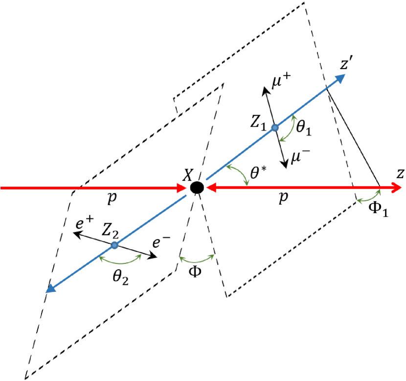
Figure 1: Definitions of the CP-sensitive final state angular observables in $gg\to H\to ZZ\to 4l$ decay.

A complimentary approach is based on studies of angular-function asymmetries arising in the case of CP violation. There are six observable functions proposed in asymmetries . The first angular observable function is defined as follows:

$$O_{1}=\frac{(\vec{p}_{2Z}-\vec{p}_{1Z})\cdot(\vec{p}_{3H}+\vec{p}_{4H})}{|\vec{p}_{2Z}-\vec{p}_{1Z}||\vec{p}_{3H}+\vec{p}_{4H}|}\;.$$

Here $\vec{p}_{i}$, $i=1,\ldots 4$ are the 3-momenta of the final state leptons in the order $l_{1}\bar{l}_{1}l_{2}\bar{l}_{2}$. The subscripts $Z$ and $H$ denote that the corresponding 3-vector is taken in the $Z$ or in the Higgs boson rest frames. Using these definitions, the second observable function reads:

$$O_{2}=\frac{(\vec{p}_{2Z}-\vec{p}_{1Z})\cdot(\vec{p}_{4H}\times\vec{p}_{3H})}{|\vec{p}_{2Z}-\vec{p}_{1Z}||\vec{p}_{4H}\times\vec{p}_{3H}|}\;.$$

The third observable function $O_{3}$ is constructed using $O_{1}$:

$$O_{3}=O_{1}\,O_{3a}\,O_{3b}\;,$$

where

$$O_{3a}=\frac{(\vec{p}_{4Z}-\vec{p}_{3Z})\cdot(\vec{p}_{1H}\times\vec{p}_{2H})}{|\vec{p}_{4Z}-\vec{p}_{3Z}||\vec{p}_{1H}\times\vec{p}_{2H}|}\;$$

and

$$O_{3b}=\frac{(\vec{p}_{3Z}-\vec{p}_{4Z})\cdot(\vec{p}_{1H}+\vec{p}_{2H})}{|\vec{p}_{3Z}-\vec{p}_{4Z}||\vec{p}_{1H}+\vec{p}_{2H}|}\;.$$

The remaining three observable functions are given by:

$$O_{4}=\frac{[(\vec{p}_{3H}\times\vec{p}_{4H})\cdot\vec{p}_{1H}][(\vec{p}_{3H}\times\vec{p}_{4H})\cdot(\vec{p}_{1H}\times\vec{p}_{2H})]}{|\vec{p}_{3H}+\vec{p}_{4H}|^{2}|\vec{p}_{1H}+\vec{p}_{2H}||\vec{p}_{3Z}-\vec{p}_{4Z}|^{2}|\vec{p}_{1Z}-\vec{p}_{2Z}|^{2}/16}\;,$$

$$O_{5}=\frac{[(\vec{p}_{4H}\times\vec{p}_{3H})\cdot\vec{p}_{1H}][(\vec{p}_{1Z}-\vec{p}_{2Z})\cdot\vec{p}_{3Z}]}{|\vec{p}_{3H}+\vec{p}_{4H}||\vec{p}_{3Z}-\vec{p}_{4Z}|^{2}|\vec{p}_{1Z}-\vec{p}_{2Z}|^{2}/8}\;,$$

and

$$O_{6}=\frac{[(\vec{p}_{1Z}-\vec{p}_{2Z})\cdot(\vec{p}_{3H}+\vec{p}_{4H})][(\vec{p}_{3H}\times\vec{p}_{4H})\cdot\vec{p}_{1H}]}{|\vec{p}_{1Z}-\vec{p}_{2Z}|^{2}|\vec{p}_{3H}+\vec{p}_{4H}|^{2}|\vec{p}_{3Z}-\vec{p}_{4Z}|/4}\;.$$

These observables are related to the final state angular variables defined in JHU2 and illustrated in Fig. 1. For instance, a trivial calculation yeilds: $O_{1}=\cos\theta_{1}$ and $O_{2}=-\sin\phi\sin\theta_{1}$.

Note that the total cross section is CP even (no interference between CP-even and CP-odd terms) and cannot be used to detect the presence of CP violating terms in the $HZZ$ vertex.

III Spin-0 model and Monte Carlo production

The dominant Higgs boson production mechanism at the LHC is gluon-fusion. To simulate the production of a Higgs-like boson and its consequent decay into $ZZ$ and $4l$, the MadGraph5 Monte Carlo generator Alwall:2011uj was used. This generator implements the Higgs Characterisation model Artoisenet:2013puc . The corresponding effective Lagrangian describing the interaction of the spin-$0$ Higgs-like boson with vector bosons is given by:

$${\cal L}_{0}^{V}=\bigg{\{} c_{\alpha}\kappa_{\rm SM}\big{[}\frac{1}{2}g_{HZZ}\,Z_{\mu}Z^{\mu}+g_{HWW}\,W^{+}_{\mu}W^{-\mu}\big{]}$$

$$\mkern-40.0mu-\frac{1}{4}\big{[}c_{\alpha}\kappa_{H\gamma\gamma}g_{H\gamma\gamma}\,A_{\mu\nu}A^{\mu\nu}+s_{\alpha}\kappa_{A\gamma\gamma}g_{A\gamma\gamma}\,A_{\mu\nu}\widetilde{A}^{\mu\nu}\big{]}$$

$$\mkern-40.0mu-\frac{1}{2}\big{[}c_{\alpha}\kappa_{HZ\gamma}g_{HZ\gamma}\,Z_{\mu\nu}A^{\mu\nu}+s_{\alpha}\kappa_{AZ\gamma}g_{AZ\gamma}\,Z_{\mu\nu}\widetilde{A}^{\mu\nu}\big{]}$$

$$\mkern-40.0mu-\frac{1}{4}\big{[}c_{\alpha}\kappa_{Hgg}g_{Hgg}\,G_{\mu\nu}^{a}G^{a,\mu\nu}+s_{\alpha}\kappa_{Agg}g_{Agg}\,G_{\mu\nu}^{a}\widetilde{G}^{a,\mu\nu}\big{]}$$

$$\mkern-40.0mu-\frac{1}{4}\frac{1}{\Lambda}\big{[}c_{\alpha}\kappa_{HZZ}\,Z_{\mu\nu}Z^{\mu\nu}+s_{\alpha}\kappa_{AZZ}\,Z_{\mu\nu}\widetilde{Z}^{\mu\nu}\big{]}$$

$$\mkern-40.0mu-\frac{1}{2}\frac{1}{\Lambda}\big{[}c_{\alpha}\kappa_{HWW}\,W^{+}_{\mu\nu}W^{-\mu\nu}+s_{\alpha}\kappa_{AWW}\,W^{+}_{\mu\nu}\widetilde{W}^{-\mu\nu}\big{]}$$

$$\mkern-40.0mu-\frac{1}{\Lambda}c_{\alpha}\big{[}\kappa_{H\partial\gamma}\,Z_{\nu}\partial_{\mu}A^{\mu\nu}+\kappa_{H\partial Z}\,Z_{\nu}\partial_{\mu}Z^{\mu\nu}$$

$$\mkern-40.0mu+\big{(}\kappa_{H\partial W}\,W_{\nu}^{+}\partial_{\mu}W^{-\mu\nu}+h.c.\big{)}\big{]}\bigg{\}}X\,,$$ (3)

where $\Lambda$ is the new physics energy scale and the field strength tensors are defined as follows:

$$V_{\mu\nu} =\partial_{\mu}V_{\nu}-\partial_{\nu}V_{\mu}\quad(V=A,Z,W^{\pm})\,,$$

$$G_{\mu\nu}^{a} =\partial_{\mu}G_{\nu}^{a}-\partial_{\nu}G_{\mu}^{a}+g_{s}f^{abc}G_{\mu}^{b}G_{\nu}^{c}\,.$$

The dual tensor $\widetilde{V}_{\mu\nu}$ is defined as:

$$\widetilde{V}_{\mu\nu}=\frac{1}{2}\epsilon_{\mu\nu\rho\sigma}V^{\rho\sigma}.\,$$

The mixing angle $\alpha$ allows the production and decay of CP-mixed states and implies CP violation when $\alpha\neq 0$ or $\alpha\neq\pi/2$. The definitions of effective tensor couplings $g_{XVV^{\prime}}$ are shown in Table 1.

	$ZZ/WW$	$\gamma\gamma$	$Z\gamma$	$gg$
$v\cdot g_{HVV^{\prime}}$	$2m_{Z/W}^{2}$	$\frac{47\alpha_{\rm EM}}{18\pi}$	$C\frac{94\cos^{2}\theta_{W}-13}{9\pi}$	$-\frac{\alpha_{s}}{3\pi}$
$v\cdot g_{AVV^{\prime}}$	0	$\frac{4\alpha_{\rm EM}}{3\pi}$	$2C\frac{8\cos^{2}\theta_{W}-5}{3\pi}$	$\frac{\alpha_{s}}{2\pi}$

Table 1: Definitions of effective tensor couplings $g_{XVV^{\prime}}$ introduced in Eq. (3) in units of the Higgs vacuum expectation $v$. The symbol $C$ is defined as: $C=\sqrt{\frac{\alpha_{\rm EM}G_{F}m_{Z}^{2}}{8\sqrt{2}\pi}}$.

The Lagrangian in Eq. (3) is an effective Lagrangian with $U(1)_{EM}$ symmetry. It parametrizes all possible Lorentz structures, is not $SU(2)\times U(1)$ invariant and does not assume that the Higgs boson belongs to a doublet of the weak $SU(2)$ group. Interaction terms corresponding to a Lagrangian of this type do not necessarily form a complete basis. However, this form is convenient for analysis of experimental data, as it relates in a simple way effective couplings and quantities observed in experiments. Note that there is a different and very popular EFT approach  Grzadkowski:2010es to studies of the Higgs boson sector based on a complete set of operators of dimension six (the so-called Warsaw basis).

The relations between parameters of the Lagrangian of Eq. (3) and tensor couplings of the effective amplitude of Eq. (2) can be derived from Feynman rules. The corresponding conversion coefficients are shown in Table 2.

Coupling	ZZ	WW	$\gamma\gamma$	Z $\gamma$	$gg$
$g_{1}$/$2ic_{a}$	$k_{SM}$	$k_{SM}$	-	-	-
$g_{2}$/$2ic_{a}$	$\tilde{K}_{HZZ}$	$\tilde{K}_{HWW}$	$\tilde{K}_{H\gamma\gamma}$	$\tilde{K}_{HZ\gamma}$	$\tilde{K}_{Hgg}$
$g_{4}$/$2is_{a}$	$\tilde{K}_{AZZ}$	$\tilde{K}_{AWW}$	$\tilde{K}_{A\gamma\gamma}$	$\tilde{K}_{AZ\gamma}$	$\tilde{K}_{Agg}$
$g^{{}^{\prime\prime}}_{1}$/$2ic_{a}$	$\tilde{K}_{H\partial Z}$	$Re(\tilde{K}_{H\partial W})$	-	-	-
$g^{{}^{\prime\prime\prime}}_{1}$/$2ic_{a}$	-	$iIm(\tilde{K}_{H\partial W})$	-	-	-

Table 2: Conversion coefficients between parameters of the Lagrangian of Eq. (3) and tensor couplings of the effective amplitude of Eq. (2).

In this table the following definitions are used:

$$\tilde{K}_{XVV^{\prime}}=\frac{1}{4}\frac{v}{\Lambda}\tilde{g}_{XVV^{\prime}}k_{XVV^{\prime}},$$

$$\tilde{K}_{H\partial V}=\frac{1}{2}\frac{v}{\Lambda}\left(\frac{\Lambda_{1}}{m_{V}}\right)^{2}k_{H\partial V},$$

$$c_{\alpha}=\cos\alpha,\;{\rm and}\;s_{\alpha}=\sin\alpha.$$

Here $X$ denotes either $H$ or $A$ and the index $VV^{\prime}$ denotes the final state gauge boson pair. The effective couplings $\tilde{g}_{XVV^{\prime}}$ are defined as follows:

• In the case of $ZZ$ or $WW$ interactions, $\tilde{g}_{XVV^{\prime}}=1$;

• For $\gamma\gamma$, $Z\gamma$ and $gg$ interactions, couplings $\tilde{g}_{XVV^{\prime}}$ are equivalent to the couplings $g_{XVV^{\prime}}$ defined in Table 1.

The couplings $\tilde{K}_{H\partial V}$, where $V=W,Z,\gamma$, correspond to the so-called contact terms of the Higgs Characterisation Lagrangian of Eq. (3). These contact terms can be reproduced in the amplitude of Eq. (2) by re-parametrising the $g_{1}$ coupling in the following form JHU_manual :

$$g_{1}\left(q^{2}_{1},q^{2}_{2}\right)=g_{1}^{SM}+g^{{}^{\prime}2}_{1}\frac{\left|q_{1}^{2}\right|+\left|q_{2}^{2}\right|}{\Lambda_{1}^{2}}+g^{{}^{\prime}3}_{1}\frac{\left|q_{1}^{2}\right|-\left|q_{2}^{2}\right|}{\Lambda_{1}^{2}}.$$

This equation represents the leading terms of the form factor expansion. In the case of complex $k_{H\partial W}$, the momenta of the $W$ bosons should be assigned as follows: $q_{1}$ for $W^{-}$ and $q_{2}$ for $W^{+}$. In the case of $HZ\gamma$ interaction with a real photon, the term proportional to $k_{H\partial\gamma}$ vanishes.

In the following we will consider a model based on the Lagrangian of Eq. (3) in which the mixing is provided by the simultaneous presence of the Standard model CP-even term and a non-Standard model CP-odd term in the $HZZ$ decay vertex. The signal Monte Carlo samples used in this analysis are produced using the Higgs Characterisation model parameters presented in Table 3.

$k_{SM}$	$k_{HZZ}$	$k_{AZZ}$	$k_{Hgg}$	$k_{Agg}$	$\Lambda,GeV$
$1$	$0$	$28.6$	$1$	$1$	$10^{3}$

Table 3: Parameters of Higgs Characterisation model used for Monte-Carlo simulation of signal samples.

The coefficient $k_{AZZ}$ was chosen such that it provided equal cross sections for decays of CP-odd and CP-even Higgs states: $\sigma(c_{\alpha}=0)=\sigma(c_{\alpha}=1)$. The tensor couplings for the decay vertex corresponding to the amplitude of Eq. (2) can be restored using the following relations: $g_{2}=2ic_{\alpha}$ and $g_{4}=2is_{\alpha}\tilde{K}_{AZZ}$, where $\tilde{K}_{AZZ}=1.76$. It is noted that the factor $2i$ is not important in the study of asymmetries because it defines the overall cross-section normalisation.

The signal samples were produced using the MadGraph5 Monte Carlo generator Alwall:2011uj . These samples were created in the range of mixing angles $-1\leq\cos\alpha\leq 1$ in steps of $0.05$. The dominant background processes $q\bar{q}\to ZZ,Z\gamma$ were also simulated with MadGraph5.

After simulation of signal and background events at $\sqrt{s}=14$ TeV, the parton showering was performed using the PYTHIA6 Monte Carlo generator pythia . Generic detector effects were included by using the PGS package Alwall:2011uj . The main detector parameters used for this simulation are presented in Table 4.

Parameter	Value
Electromagnetic calorimeter resolution $\cdot\sqrt{E}$	0.1
Hadronic calolrimeter resolution$\cdot\sqrt{E}$	0.8
MET resolution	0.2
Outer radius of tracker (m)	1.0
Magnetic field (T)	2.0
Track finding efficiency	0.98
Tracking $\eta$ coverage	2.5
$e/\gamma$ $\eta$ coverage	2.8
Muon $\eta$ coverage	2.8

Table 4: Tuning parameters used to simulate detector effects with PGS package.

For comparison, the expected acceptance, efficiencies and resolutions of the ATLAS and CMS detectors of the LHC can be found in  ATLAS_paper ; CMS_paper .
Finally a kinematic selection was applied. It was required that candidates decayed to two same flavour oppositely charged lepton pairs. If several of such candidates could be reconstructed in an event, the leptons pairs with invariant masses closest to the on-shell Z mass where chosen. Each individual lepton had a psudorapidity $|\eta|<2.5$ and transverse momentum $p_{T}>7~{}$GeV. The most energetic lepton should satisfy $p_{T}>20~{}$GeV whereas the second (third) similarly had $p_{T}>15~{}$GeV ($p_{T}>10~{}$GeV). The invariant mass of the on-shell Z boson was in the mass window $(50,106)~{}$GeV while the off-shell Z boson $m_{Z*}>20~{}$GeV. Only Higgs candidates in the signal region $115~{}$GeV$<m_{H}<130~{}$GeV where considered. The selection is a simplified version of the one presented in  atlas_higgs .

IV Asymmetries

For each observable $O_{i}$ sensitive to CP violation, the corresponding asymmetry can be defined as:

$$A_{i}=\frac{N(O_{i}>0)-N(O_{i}<0)}{N(O_{i}>0)+N(O_{i}<0)},$$ (4)

where $N$ is the number of events with the observable less or greater than zero. Integrating the corresponding decay probabilities, it can be shown that these asymmetries directly probe the tensor couplings defined in the amplitude of Eq. (2) asymmetries . The value of $A_{1}$ is proportional to $Im(g_{4})$, while $A_{2},A_{3},A_{4},A_{5}$ and $A_{6}$ probe the values of $Re(g_{4})$ and $Im(g_{2})$ respectively.

Analysis of asymmetries sensitive to CP-violation for the process of Eq. (1) was performed in asymmetries . In this section we extend this analysis by including effects of parton showering, hadronization, generic detector effects and contributions from the irreducible $q\bar{q}\to ZZ/Z\gamma\to 4l$ background. Lepton interference in the final state and the contribution of two off-shell $Z$-bosons are also taken into account.

The distributions of observables $O_{2},O_{3},O_{4}$ and $O_{5}$ for two values of the mixing angle $\cos\alpha=1$ and $\cos\alpha=0.5$ are shown in Fig. 2.

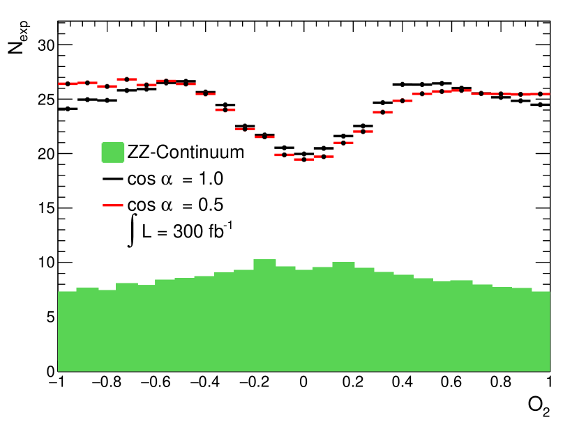
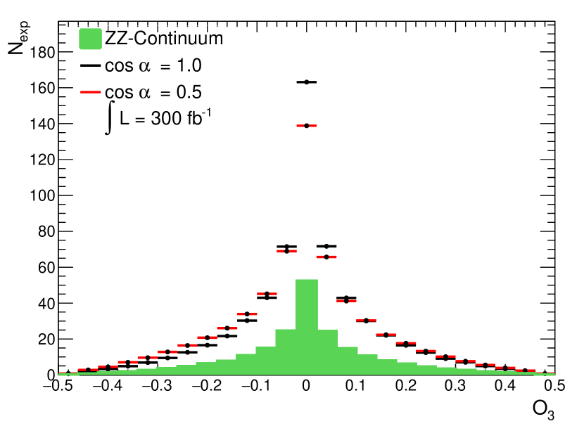
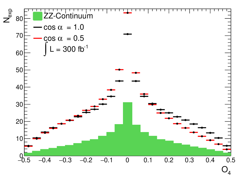
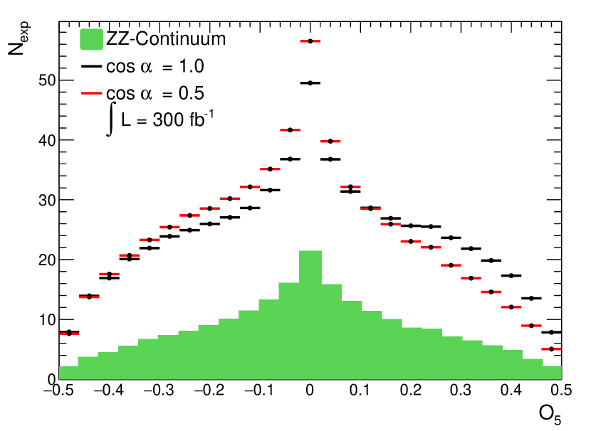
Figure 2: Distributions of observables $O_{2},O_{3},O_{4}$ and $O_{5}$ for two values of the mixing angle $\alpha$.

Signal $H\to ZZ\to 4l$ events are generated using the production and decay model defined in Table 3. The contributions from the signal and $q\bar{q}\to ZZ\to 4l$ background are normalised to their respective expectations at $300fb^{-1}$. It is noted that the presence of CP-mixing leads to distortions of distributions of selected observables. The distributions of $O_{2}$ through $O_{5}$ become asymmetric in the presence of a real component of $g_{4}$. This asymmetry is especially pronounced for $O_{4}$ and $O_{5}$. As suggested in asymmetries , the background is CP conserving and the corresponding distributions of observables are symmetric. The shapes of asymmetries $A_{i}$ for the model presented in Table 3 are shown in Fig. 3.

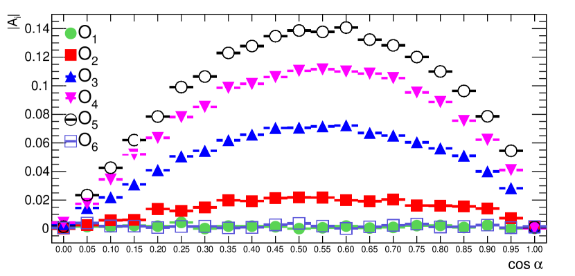
Figure 3: Asymmetries generated for observables $O_{i}$.

The pure CP-even and CP-odd cases are given by $\cos\alpha=1$ and $\cos\alpha=0$, respectively.

Note, that according to the structure of Lagrangian (Eq. (3)) the CP-violating contribution is defined by the parameter $p=\tilde{K}_{AZZ}\tan\alpha$. This parameter thus determines the corresponding asymmetries of angular observables. Knowing the distribution of asymmetries for given $\tilde{K}_{AZZ}$ it is possible to obtain the corresponding distributions for any $\tilde{K}_{AZZ}$ by using the condition $p=const$.

It is noted, that for the physics model used in this study, the observables $O_{1}$ and $O_{6}$ do not generate asymmetries visible with the current Monte Carlo sample. The consistency of these asymmetries with zero confirms that additional effects that are taken into account in our work such as lepton interference, off-shell $ZZ$ production, $ZZ$ background, experimental cuts and detector acceptance do not produce an artificial asymmetry not related with the presence of CP-odd terms. The asymmetric behaviour is clearly visible for $O_{2}$ through $O_{5}$. The asymmetries for $O_{4}$ and $O_{5}$ calculated using Eq. (4) may exceed $10\%$ .

In Fig. 3 asymmetry plots are given for $\cos\alpha$ in the range from $0$ to $1$. For negative $\cos\alpha$ the asymmetries change sign but keep the same shape. This property allows using the asymmetry approach to measure the relative phase in the amplitude of Eq. (2).

The significance of the expected asymmetry can be estimated as:

$$S=\Delta N/\sqrt{N}=A_{i}N_{S}/\sqrt{N},$$

where $N=N_{S}+N_{B}$ is the total number of signal and background events and $\Delta N$ is the difference in the number of events with $O_{i}<0$ and $O_{i}>0$. It is also noted that $\Delta N\approx\Delta N_{S}$, because the $ZZ$ background does not contribute to asymmetries at leading order. Following the results of the simulation presented in  ATLAS-Collaboration:2013jwa , the number of signal and background events at $\sqrt{s}=14$ TeV can be estimated as: $N_{S}=1.32L$ and $N_{B}=0.71L$ respectively. Here $L$ represents the integrated luminosity in ${\rm fb}^{-1}$. A dataset with the integrated luminosity of $300\;{\rm fb}^{-1}$ is expected to be collected during the Run III of the LHC.

Using the above expressions, one can estimate an expected asymmetry of about $9.5\%$ to be measured with this data sample. The corresponding significance will be around two standard deviations. The region $0.340<\cos\alpha<0.789$ will then be excluded at $95\%$ CL.

This exclusion range can be expressed in terms of $f_{g_{4}}$ fraction of events Khachatryan:2014kca arising from the anomalous coupling $g_{4}$:

$$f_{g_{4}}=\frac{\sigma_{4}|g_{4}|^{2}}{\sigma_{1}|g_{1}|^{2}+\sigma_{4}|g_{4}|^{2}},$$ (5)

where $g_{i}$ are couplings of the decay vertex, and $\sigma_{i}$ is the cross section of the processes $H\to ZZ\to 4l$ corresponding to $g_{i}=1,g_{i\neq j}=0$. Eq. (5) can be rewritten in terms of the mixing angle $\alpha$ as:

$$f_{g_{4}}=\frac{1}{1+\frac{\sigma_{1}}{\sigma_{4}}\,\left(\frac{k_{SM}}{\tilde{K}_{AZZ}}\right)^{2}\cot^{2}\alpha},$$

where the ratio of cross sections $\sigma_{4}/\sigma_{1}=0.139$ is obtained from the Monte Carlo generator.

The range of the fraction of events of Eq. (5) close to $1$ has been already excluded by CMS Khachatryan:2014kca . Taking this into account, the exclusion limit obtained in the presented analysis becomes $f_{g_{4}}<0.206$ at $300\;{\rm fb}^{-1}$ for the model described by the Lagrangian of Eq. (3) and parameters given in Table 3.

For the high luminosity LHC, assuming the same signal and background yields per fb as above, the following exclusion range can be established: $0.089<\cos\alpha<0.968$ at $95\%$ CL. This corresponds to an upper limit $f_{g_{4}}=0.028$ at $3000\;{\rm fb}^{-1}$.

In the same way as above, we performed estimates for four more values of the model parameter $\tilde{K}_{AZZ}$. Monte Carlo samples were generated for each point of two dimensional model space $(\cos\alpha,\tilde{K}_{AZZ})$. The number of signal events was calculated as $N_{S}=N_{S}^{SM}\sigma/\sigma^{SM}$ assuming constant K-factors. The results are presented in Table 5. These limits on $f_{g_{4}}$ are close to the ones expected in ATLAS ATLAS-Collaboration:2013jwa and CMS Khachatryan:2014kca experiments.

$L,\;{\rm fb}^{-1}$	$300$		$3000$
$\tilde{K}_{AZZ}/1.76$	$\Delta c_{\alpha}$	$f_{g_{4}}$	$\Delta c_{\alpha}$	$f_{g_{4}}$
0.6	-	-	0.122-0.921	0.026
0.8	0.431-0.650	0.274	0.100-0.953	0.027
1.0	0.340-0.789	0.207	0.089-0.968	0.028
1.2	0.307-0.852	0.191	0.087-0.975	0.031
1.4	0.297-0.886	0.188	0.086-0.981	0.032

Table 5: Upper limit on $f_{g_{4}}$ and $\cos\alpha$ range excluded at the $95\%$ CL.

The region of $\tilde{K}_{AZZ}/1.76$ above 1.4 is not considered. In this region the cross sections exceed the SM cross section by more than a factor of two.

In Figs. 4 and 5 the regions of model parameter space ($c_{\alpha}$, $\tilde{K}_{AZZ}$) excluded by the current analysis are shown. The shadowed areas are excluded at the $95\%$ CL. Lines in Figs. 4 and 5 represent a polinomial fit to the results of the method of asymmetries.

Note that CP-odd observables were studied also in Buchalla:2013mpa . According to this article the detection of CP-violating effects is out of reach of the LHC. However, as was mentioned in Buchalla:2013mpa , these effects might in principle attain large values because of numerical enhancements.

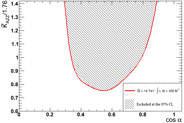
Figure 4: The $95\%$ CL exclusion limits for model parameters $c_{\alpha}$, $\tilde{K}_{AZZ}$ at $300fb^{-1}$. Regions of rejected model parameters are shown.

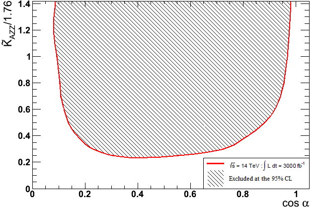
Figure 5: The $95\%$ CL exclusion limits for model parameters $c_{\alpha}$, $\tilde{K}_{AZZ}$ at $3000fb^{-1}$. Regions of rejected model parameters are shown.

V Mixing angle observable fit

The asymmetries $A_{i}$ discussed in the Section IV are integrated quantities of angular observables $O_{i}$ and thus provide limited information about the anomalous contributions to the $HZZ$ vertex. The optimal sensitivity to these contributions can be obtained by studying the shapes of distributions of observables $O_{i}$ and their correlations.

The sensitivity of individual observables to the presence of anomalous contributions to the $HZZ$ vertex is studied by fitting the shape of these observables as a function of the mixing angle. The likelihood function of the fit is defined as:

$$\mathcal{L}(\cos{\alpha},\mu,\theta)=\prod_{j}^{\mathrm{N_{chan}}}\prod_{i}^{\mathrm{N_{bin}}}P(N_{i,j}|\mu_{j}\cdot S_{i,j}(\cos{\alpha},\theta)+B_{i,j}(\theta)).$$

Here besides the parameter of interest $\cos{\alpha}$, two nuisance parameters have been introduced: the best fitting signal strength $\mu$ and a systematic normalization uncertainty $\theta$. The likelihood function is a product over the different final states and bins of the specific observable that is being fitted. In each bin, the observed number of events from pseudo-data $N$, is compared to the expected number of events of the model $S+B$ assuming a Poissonian distribution of entries $P$. By varying the mixing parameter $\cos{\alpha}$ of the likelihood for a given dataset we can construct the standard log-likelihood test statistic:

$$-2\ln\Lambda(\cos{\alpha})=-2\ln\frac{\mathcal{L}(\cos{\alpha})}{\mathcal{L}(\cos{\hat{\alpha}})},$$

where $\hat{\alpha}$ denotes the mixing angle that maximises the likelihood function over the scan. The other likelihood parameters are profiled at the corresponding $\cos{\alpha}$ value. The 95$\%$ exclusion is reached when $-2\ln\Lambda(\cos{\alpha})>3.84$. The definitions of the $64\%$ CL and $95\%$ CL exclusion regions is demonstrated in Fig. 6.

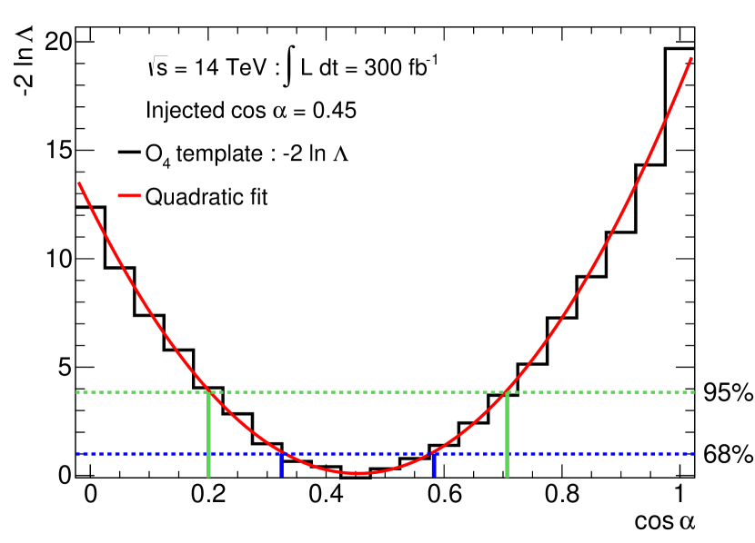
Figure 6: Example of the likelihood curve for the mixing angle observable fit of $O_{4}$. The definitions of the $64\%$ CL and $95\%$ CL exclusion regions are demonstrated.

Results of the scan of the mixing angle $\alpha$ produced with the mixing angle observable fit corresponding to the integrated luminosity of $300\;{\rm fb}^{-1}$ are presented in Fig. 7.

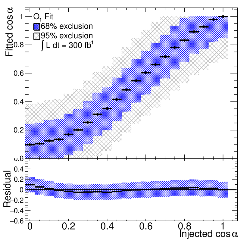
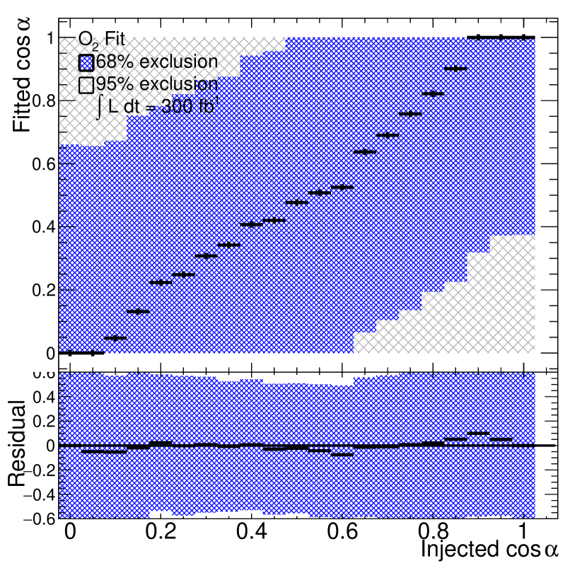
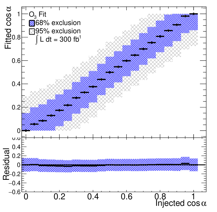
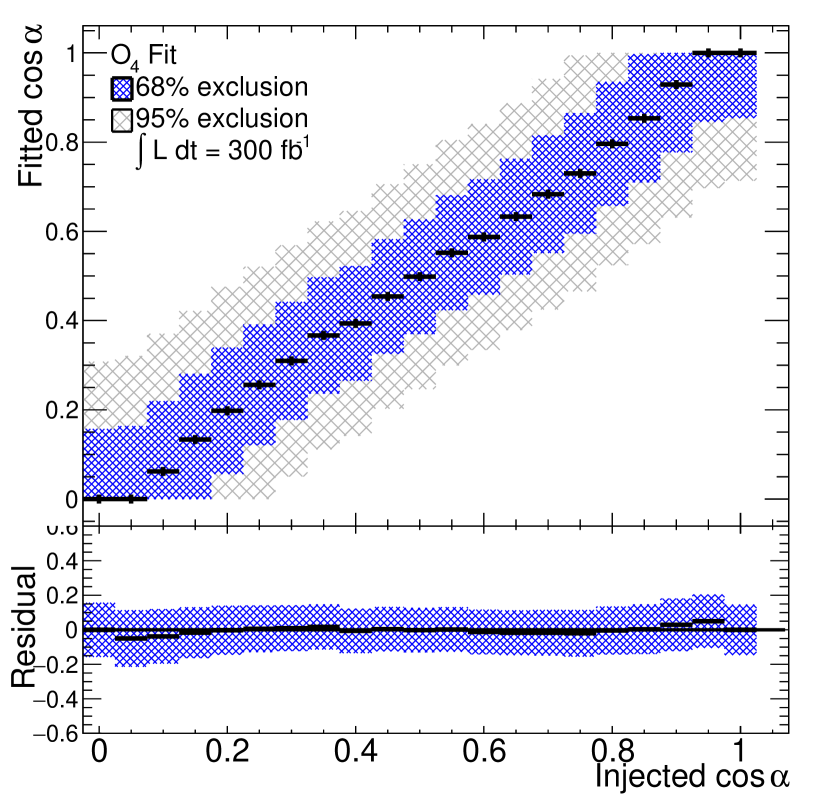
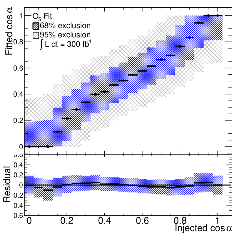
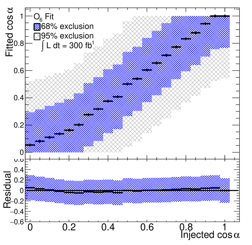
Figure 7: Results of the mixing angle $\alpha$ scan produced with the mixing angle observable fit corresponding to the integrated luminosity of $300\;{\rm fb}^{-1}$.

The results are reported for the model with $\tilde{K}_{AZZ}=1.76$ and remaining parameters as defined in Table 3. The values of the mixing angle $\cos\alpha$ used to generate the input pseudo-data are marked on the $x$-axis. Every bin of the injected $\cos\alpha$ on represents the null-hypothesis likelihood curve similar to Fig. 6. The $y$-axis shows the $\cos\hat{\alpha}$ values reconstructed in the fit. The blue and grey dashed areas represent the $64\%$ CL and $95\%$ CL limits respectively. The white area in each bin of injected $\cos\alpha$ is excluded at $95\%$ CL. As expected, the sensitivity to the mixing angle varies for different observables, resulting in significantly different exclusion regions. The weakest exclusion is reached with the $O_{2}$, while the strongest is reached with the $O_{4}$.

The results corresponding to the integrated luminosity of $3000\;{\rm fb}^{-1}$ are presented in Fig. 8.

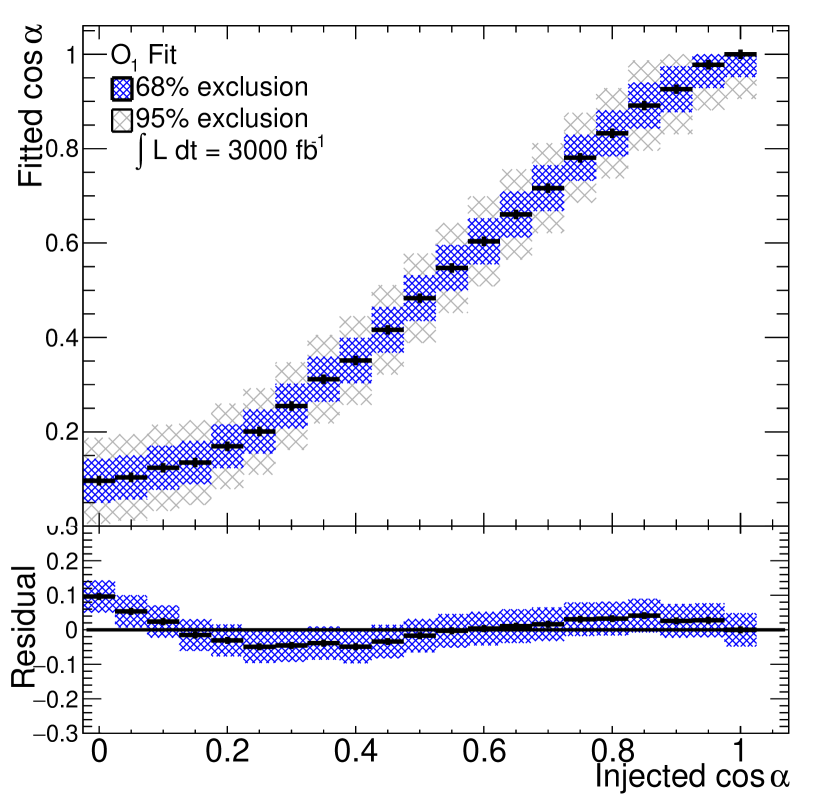
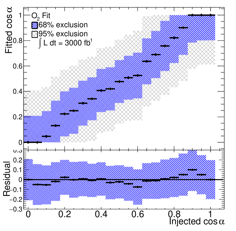
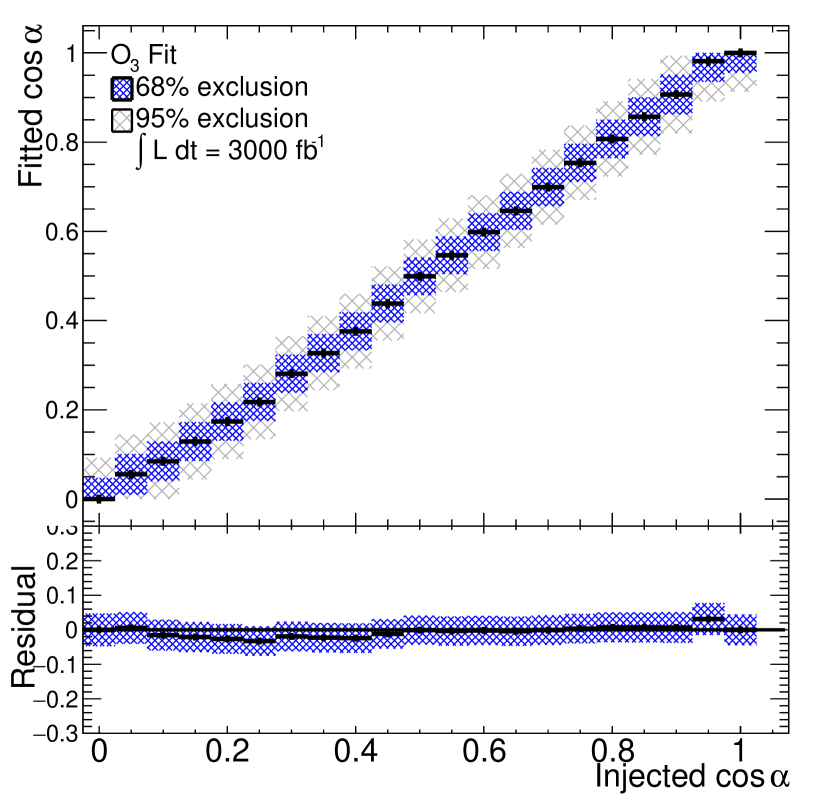
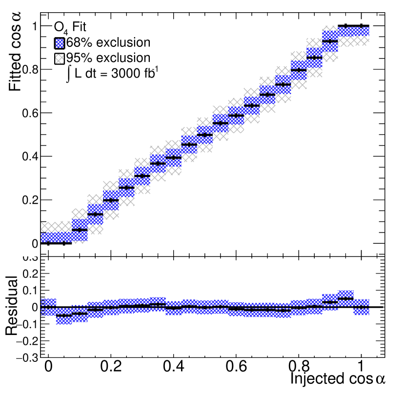
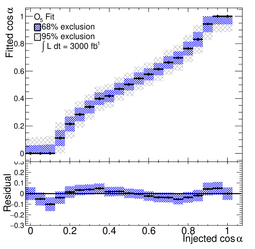
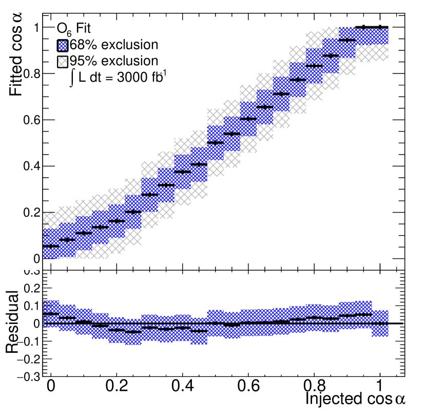
Figure 8: Results of the mixing angle $\alpha$ scan produced with the mixing angle observable fit corresponding to the integrated luminosity of $3000\;{\rm fb}^{-1}$.

Compared to $300\;{\rm fb}^{-1}$, the $95\%$ CL exclusion regions around the fitted $\cos\hat{\alpha}$ values are significantly reduced. Assuming the pure Standard Model signal, the following exclusion limits can be set using the $O_{4}$ observable alone: $0<\cos\hat{\alpha}<0.708$ at the $95\%$ CL for $300\;{\rm fb}^{-1}$ and $0<\cos\hat{\alpha}<0.908$ at the $95\%$ CL for $3000\;{\rm fb}^{-1}$. The exclusion limits obtained from other observables assuming the Standard Model signal are reported in Table 6.

The exclusion limits obtained for hypothetical BSM signals can be read from Fig. 7 and 8. It is noted that by fitting the shape of the $O_{4}$ observable alone the exclusion limits similar to those reported in the Section IV can be obtained. Further improvements can be obtained by combining several observables in the same fit.

$L,\;{\rm fb}^{-1}$	$300$		$3000$
Observable	$\Delta c_{\alpha}$	$f_{g_{4}}$	$\Delta c_{\alpha}$	$f_{g_{4}}$
$O_{1}$	0 - 0.695	0.315	0 - 0.903	0.089
$O_{2}$	-	-	0 - 0.604	0.428
$O_{3}$	0 - 0.719	0.287	0 - 0.911	0.081
$O_{4}$	0 - 0.708	0.300	0 - 0.908	0.084
$O_{5}$	0 - 0.631	0.394	0 - 0.883	0.108
$O_{6}$	0 - 0.533	0.520	0 - 0.852	0.104

Table 6: Upper limit on $f_{g_{4}}$ and $\cos\alpha$ range excluded at the $95\%$ CL with the mixing angle observable fit. The Standard Model signal is assumed. The BSM templates are generated according to the model defined in Table 3 with $\tilde{K}_{AZZ}=1.76$.

VI Conclusion

In this article studies of tensor structure of the $HZZ$ vertex are presented. The investigation is performed using the $pp\to H\to ZZ\to 4l$ process assuming the gluon fusion production of the spin-0 resonance. The background contributions, detector resolution, trigger and selection efficiencies expected for the LHC are taken into account. Two different approaches to detect CP-violation effects in the $HZZ$ vertex were used. The first approach is based on a simple counting experiment for angular asymmetries of CP-sensitive observables. It was shown that the presence of CP violating terms may result in angular asymmetries exceeding $10\%$. The $95\%$ CL exclusion ranges for the mixing angle at different parameters of spin-0 Higgs boson model including the Standard Model CP-even term and anomalous CP-odd term $g_{4}$ are calculated. These results are also presented in terms of the effective cross section fraction $f_{g_{4}}$. The obtained limits are comparable with the ATLAS and CMS projections for Run III at the LHC and the High-Luminosity LHC presented in  Khachatryan:2014kca ; ATLAS-Collaboration:2013jwa .

The sensitivity of individual observables to the presence of anomalous contributions to the $HZZ$ vertex was studied by fitting the shape of these observables as a function of the mixing angle. It is demonstrated that using a single most sensitive observable, this approach gives $f_{g_{4}}$ limits comparable with asymmetries method and with the ATLAS and CMS projections. Compared to the method of angular asymmetries, this approach has an advantage of using the complete shape information of CP-odd observables. It is demonstrated that some of the observables, that do not generate significant angular asymmetry in presence of significant CP-mixing, can still provide restrictive $f_{g_{4}}$ limits when their complete shape is analysed. Combining several CP-odd observables in the same fit or combining several angular asymmetries would likely further improve sensitivity to the CP violating coupling. It is noted that careful experimental investigation of all observables, even not the leading ones, is important, since they probe different terms of the $HZZ$ vertex.

References

- (1) CMS Collaborations, Phys. Lett. B 716, 30 (2012).
- (2) ATLAS Collaborations, Phys. Lett. B 716, 1 (2012).
- (3) ATLAS Collaborations, Phys. Lett. B 726, 88 (2013).
- (4) CMS Collaboration, (2014), arXiv:1411.3441.
- (5) CMS Collaboration, Phys. Rev. Lett. 110, 081803 (2013).
- (6) ATLAS Collaborations, Phys. Lett. B 726, 120 (2013).
- (7) D. Chang, W.-Y. Keung, and I. Phillips, Phys. Rev. D 48, 3225 (1993).
- (8) B. Grzadkowski and J. Gunion, Phys. Lett. B 350, 218 (1995).
- (9) J. F. Gunion, B. Grzadkowski, and X.-G. He, Phys. Rev. Lett. 77, 5172 (1996).
- (10) B. Grzadkowski, J. F. Gunion, and J. Kalinowski, Phys. Rev. D 60, 075011 (1999).
- (11) B. Grzadkowski, J. F. Gunion, and J. Pliszka, Nucl. Phys. B583, 49 (2000).
- (12) T. Plehn, D. L. Rainwater, and D. Zeppenfeld, Phys. Rev. Lett. 88, 051801 (2002).
- (13) S. Choi, D. Miller, M. Muhlleitner, and P. Zerwas, Phys. Lett. B 553, 61 (2003).
- (14) C. Buszello, I. Fleck, P. Marquard, and J. van der Bij, Eur. Phys. J. C 32, 209 (2004).
- (15) V. Hankele, G. Klamke, D. Zeppenfeld, and T. Figy, Phys. Rev. D 74, 095001 (2006).
- (16) R. M. Godbole, D. Miller, and M. M. Muhlleitner, JHEP 0712, 031 (2007).
- (17) W.-Y. Keung, I. Low, and J. Shu, Phys. Rev. Lett. 101, 091802 (2008).
- (18) S. Berge and W. Bernreuther, Phys. Lett. B 671, 470 (2009).
- (19) Q.-H. Cao, C. Jackson, W.-Y. Keung, I. Low, and J. Shu, Phys. Rev. D 81, 015010 (2010).
- (20) A. De Rujula, J. Lykken, M. Pierini, C. Rogan, and M. Spiropulu, Phys. Rev. D 82, 013003 (2010).
- (21) Y. Gao et al., Phys. Rev. D 81, 075022 (2010).
- (22) S. Berge, W. Bernreuther, B. Niepelt, and H. Spiesberger, Phys. Rev. D 84, 116003 (2011).
- (23) F. Bishara et al., JHEP 1404, 084 (2014).
- (24) R. Harnik, A. Martin, T. Okui, R. Primulando, and F. Yu, Phys. Rev. D 88, 076009 (2013).
- (25) S. Berge, W. Bernreuther, and H. Spiesberger, Phys. Lett. B 727, 488 (2013).
- (26) A. Menon, T. Modak, D. Sahoo, R. Sinha, and H. Cheng, Phys. Rev. D 89, 095021 (2014).
- (27) Y. Chen, R. Harnik, and R. Vega-Morales, Phys. Rev. Lett. 113, 191801 (2014).
- (28) J. S. Gainer, J. Lykken, K. T. Matchev, S. Mrenna, and M. Park, Phys. Rev. Lett. 111, 041801 (2013).
- (29) P. Avery et al., Phys. Rev. D 87, 055006 (2013).
- (30) J. S. Gainer, J. Lykken, K. T. Matchev, S. Mrenna, and M. Park, Phys. Rev. D 91, 035011 (2014).
- (31) M. Chen et al., Phys. Rev. D 89, 034002 (2014).
- (32) D. Stolarski and R. Vega-Morales, Phys. Rev. D 86, 117504 (2012).
- (33) W. Buchmuller and D. Wyler, Nucl .Phys. B 268, 621 (1986).
- (34) B. Grzadkowski, M. Iskrzynski, M. Misiak, and J. Rosiek, JHEP 1010, 085 (2010).
- (35) S. Bolognesi et al., Phys. Rev. D 86, 095031 (2012).
- (36) I. Anderson et al., Phys. Rev. D 89, 035007 (2014).
- (37) R. M. Godbole, D. J. Miller, and M. M. Muhlleitner, JHEP 0712, 031 (2007).
- (38) J. Alwall, M. Herquet, F. Maltoni, O. Mattelaer, and T. Stelzer, JHEP 1106, 128 (2011).
- (39) P. Artoisenet et al., JHEP 1311, 043 (2013).
- (40) I. Anderson et al., 2014, http://www.pha.jhu.edu/spin/- -manJHUGenerator.v4.8.1.pdf .
- (41) T. Sjostrand, S. Mrenna, and P. Z. Skands, JHEP 05, 026 (2006).
- (42) ATLAS Collaboration, JINST 3, S08003 (2008).
- (43) CMS Collaboration, JINST 3, S08004 (2008).
- (44) ATLAS Collaboration, Report No. ATL-PHYS-PUB-2013-013, 2013, http://cds.cern.ch/record/1611123 .
- (45) G. Buchalla, O. Cata, and G. D’Ambrosio, Eur .Phys. J. C 74, 2798 (2014).