Driven-dissipative Ising model: mean-field solution

Abstract

We study the fate of the Ising model and its universal properties when driven by a rapid periodic drive and weakly coupled to a bath at equilibrium. The far-from-equilibrium steady-state regime of the system is accessed by means of a Floquet mean-field approach. We show that, depending on the details of the bath, the drive can strongly renormalize the critical temperature to higher temperatures, modify the critical exponents, or even change the nature of the phase transition from second to first order after the emergence of a tricritical point. Moreover, by judiciously selecting the frequency of the field and by engineering the spectrum of the bath, one can drive a ferromagnetic Hamiltonian to an antiferromagnetically ordered phase and vice-versa.

The Ising model is undoubtedly the most studied model of statistical mechanics. Besides its equilibrium properties, its coarsening dynamics following a temperature quench from the paramagnetic to the ordered phase is also quite well understood BrayReview ; Exact2d , even in the presence of weak disorder Dziarmaga ; SAALFC ; ACLFCP . Taking into account the dissipative mechanisms due to the inevitable coupling of the spin system to an environment has been successful in the description of important many-body phenomena such as the decay of metastable phases key-30 ; key-31 ; key-32 ; key-33 ; key-34 ; key-35 , hysteretic responses key-36 ; key-37 ; key-38 and magnetization switching in mesoscale ferromagnets key-39 ; key-40 . As it is becoming clear these days that driven-dissipative physics, i.e. the balancing of non-equilibrium conditions and dissipative mechanisms, is a promising route to achieve a new type of control over matter, a burning question arises: can the Ising model be driven to non-equilibrium steady states (NESS) with enhanced or even novel properties?

This question has been approached in the context of slowly oscillating drives (magnetic fields or electrochemical potentials) by means of Monte-Carlo simulations key-35b ; key-36 ; key-37 ; key-38 ; key-47 ; key-48 ; key-49 , mean-field treatment key-41 ; key-42 ; key-43 ; key-44 ; key-45 ; key-46 , or other analytical techniques key-50 ; key-51 ; key-52 ; key-53 . One of the key results is the existence of a so-called dynamical phase transition, where the cycle-averaged magnetization becomes non-zero in a singular fashion. This has recently been supported by experimental evidence in the dynamics of thin ferromagnetic films key-54 .

In this Letter, we focus on the Ising model driven by a rapidly oscillating magnetic field $h\cos(\omega t)$. We depart from the usual Floquet engineering approach to many-body phases, mostly directed towards cold-atomic systems PolkovnikovReview , by including a dissipative mechanism, namely by weakly coupling the system to an external equilibrium bath. The properties of the latter are kept generic in order to study the influence of its spectrum on the dynamics. Dissipation is the natural counterpart of driving and our results are an unquestionable proof that the presence of a bath can have far-reaching consequences.

We access the non-equilibrium steady states by means of a Floquet mean-field approach. We derive the mean-field self-consistent equation for the magnetization and use it to derive the non-equilibrium phase diagram. Whenever analytical solutions are beyond reach, we complete the picture with numerical results. Our main results are to show how to combine drive (i.e. $h$ and $\omega$) and dissipation (i.e. mostly the low-energy spectrum of the bath) to increase the critical temperature $T_{{\rm c}}$, to modify the critical exponent $\beta_{T}$, as well as to change the order of the phase transition. Additionally, we show that the drive can, in the presence of carefully selected baths, convert a ferromagnetically ordered system to an antiferromagnetic order, and vice versa.

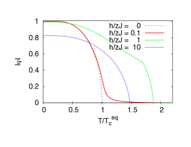
Figure 1: (color online) Mean-field magnetization $|\varphi|$ as a function of the temperature $T$ of the bath (super-Ohmic, $s=1$) for different values of the drive $h$ given in the key: $h=0$ (equilibrium), $h\ll\omega$, $h\sim\omega$ and $h\gg\omega$. The critical temperature for $h\ll\omega$, $T_{{\rm c}}=(1+s)T_{{\rm c}}^{{\rm eq}}$, is computed exactly in Eq. (16). In the temperature range $T_{{\rm c}}^{{\rm eq}}<T<T_{{\rm c}}$, $|\varphi|\sim(h/\omega)^{2/s}\omega/zJ$. ($\omega=zJ=T_{{\rm c}}^{{\rm eq}}$).

Model.

The total Hamiltonian is composed of the system, the bath and the system-bath Hamiltonians, $H(t)=H_{S}\left(t\right)+H_{B}+H_{SB}$ with (we set $\hbar=k_{{\rm B}}=1$)

$$H_{S}\left(t\right)= -J\sum_{\langle ij\rangle}\sigma_{i}^{z}\sigma_{j}^{z}-h\cos\left(\omega t\right)\sum_{i}\sigma_{i}^{z}\;,$$ (1a)

$${H}_{B}= \sum_{i,\alpha}\omega_{\alpha}\;b_{i,\alpha}^{\dagger}\,b_{i,\alpha}\;,$$ (1b)

$${H}_{SB}= \sum_{i,\alpha}t_{\alpha}\,\sigma_{i}^{x}\left(b_{i,\alpha}+b_{i,\alpha}^{\dagger}\right)\;.$$ (1c)

The spin $1/2$’s, represented at each site $i$ of the bipartite lattice by the usual Pauli operators $\sigma_{i}^{x,y,z}$, are interacting through a nearest-neighbor interaction $J$. $h$ is the strength of the periodic drive with frequency $\omega\equiv 2\pi/\tau$ (we choose $\omega\geq 0$). Equilibrium conditions are recovered for $h=0$ or $\omega=0$. Notice that in the absence of an environment, the drive has trivial consequences on the dynamics of the Ising model. Indeed, as $[\sigma_{i}^{z},H(t)]=0$ at all times, all the degrees of freedom are conserved quantities. The environment is composed of local baths expressed in terms of a collection of non-interacting bosonic modes labelled by $\alpha$, with energy $\omega_{\alpha}$ and with creation and annihilation operators given by $b_{i,\alpha}^{\dagger}$ and $b_{i,\alpha}$. Each is in equilibrium at temperature $T\equiv 1/\beta$ and we assume it is a “good bath”, i.e. it has a very large number of degrees of freedom and it remains in thermal equilibrium. Below, we replace $\sum_{\alpha}$ by $\int{\rm d}\epsilon\,\rho(\epsilon)$ where $\rho(\epsilon)$ is the bath density of state. Without loss of generality, the chemical potential is set to 0 and $\rho(\epsilon<0)=0$. $H_{{\rm SB}}$ is responsible for thermal spin flips and the parameters $t_{\alpha}$ control the strength of the spin-bath couplings. After integrating out the bath degrees of freedom, the bath will enter the reduced problem via the hybridization function $\nu(\epsilon)\equiv|t({\epsilon})|^{2}\rho\left(\epsilon\right)$. The low-energy behavior of the hybridization $\nu(\epsilon)\stackrel{{\scriptstyle[}}{{0}}<\epsilon\to 0]{}{\sim}\epsilon^{1+s}$ characterizes whether the bath is Ohmic ($s=0$), sub-Ohmic ($s<0$), or super-Ohmic ($s>0$). Note that we do not consider additional system-bath coupling terms such as $\sigma_{i}^{y,z}\,(b_{i,\alpha}+b_{i,\alpha}^{\dagger})$ because they do not induce any qualitative change in the non-equilibrium dynamics.

Floquet mean-field description.

The time-dependent mean-field Hamiltonian corresponding to $H(t)$ in Eq. (1) is the one of a single spin coupled to its local bath, and reads $\bar{H}(t)=\bar{H}_{S}\left(t\right)+\bar{H}_{B}+\bar{H}_{SB}$ with

$$\bar{H}_{S}\left(t\right)= -zJ\varphi\left(t\right)\sigma^{z}-h\sigma^{z}\cos\left(\omega t\right)\;,$$ (2a)

$$\bar{H}_{B}= \sum_{\alpha}\omega_{\alpha}\;b_{\alpha}^{\dagger}\,b_{\alpha}\;,$$ (2b)

$$\bar{H}_{SB}= \sum_{\alpha}t_{\alpha}\,\sigma^{x}\left(b_{\alpha}+b_{\alpha}^{\dagger}\right)\;.$$ (2c)

Here, $\varphi(t)$ is the expectation value of $\sigma^{z}(t)$ which serves as the order parameter, and $z$ is the coordination number of the bipartite lattice. When the coupling the bath is weak (see the discussion below), the spin subsystem can be seen as quasi-isolated during many periods of the drive. There, the Floquet theorem states that the instantaneous eigenstates of the time-periodic Hamiltonian $\bar{H}_{{\rm S}}(t)$ can be written in the form $|\psi_{\alpha}(t)\rangle={\rm e}^{-{\rm i}E_{\alpha}t}|\psi_{\alpha}^{{\rm P}}(t)\rangle$ where $E_{\alpha}$ is a so-called Floquet quasi-energy and $|\psi_{\alpha}^{{\rm P}}(t)\rangle$ is periodic: $|\psi_{\alpha}^{{\rm P}}(t+\tau)\rangle=|\psi_{\alpha}^{{\rm P}}(t)\rangle$. Owing to the fact that $\sigma^{z}$ is a conserved quantity, we may choose our Floquet eigenstates to simultaneously diagonalize $\sigma^{z}$. Note that this also implies that $\varphi(t)$ is a constant (at least between two events induced by the weakly-coupled bath). Altogether, the instantaneous eigenstates of $\bar{H}_{{\rm S}}(t)$ are simply given by

$$\left|\uparrow\!\left(t\right)\right\rangle= \,{\rm e}^{+{\rm i}\left[zJ\varphi\,t+\frac{h}{\omega}\sin\left(\omega t\right)\right]}\;\left|\uparrow\right\rangle={\rm e}^{-{\rm i}\epsilon_{\uparrow}t}\;\left|\uparrow^{{\rm P}}\!(t)\right\rangle\;,$$ (3)

$$\left|\downarrow\!\left(t\right)\right\rangle= \,{\rm e}^{-{\rm i}\left[zJ\varphi\,t+\frac{h}{\omega}\sin\left(\omega t\right)\right]}\;\left|\downarrow\right\rangle={\rm e}^{-{\rm i}\epsilon_{\downarrow}t}\;\left|\downarrow^{{\rm P}}\!(t)\right\rangle\;,$$ (4)

from which one identifies the Floquet quasi-energies and the periodic states, reading

$$\epsilon_{\uparrow}\equiv-zJ\varphi\;,\quad \left|\uparrow^{{\rm P}}\!(t)\right\rangle=\sum_{n}J_{n}\left({h}/{\omega}\right){\rm e}^{-{\rm i}n\omega t}\left|\uparrow\right\rangle\;,$$ (5)

$$\epsilon_{\downarrow}\equiv zJ\varphi\;,\quad \left|\downarrow^{{\rm P}}\!(t)\right\rangle=\sum_{n}J_{n}\left({h}/{\omega}\right){\rm e}^{+{\rm i}n\omega t}\left|\downarrow\right\rangle\;,$$ (6)

where $J_{n}$ are the Bessel functions of the first kind.

Rates.

The bath is inducing incoherent transitions between the eigenstates. The transition rate $R_{\uparrow\downarrow}$ from $\left|\uparrow\right\rangle$ to $\left|\downarrow\right\rangle$ can be obtained by means of a Floquet-Fermi golden rule key-28 :

$$R_{\uparrow\downarrow}(\varphi)=2\pi\sum_{m\in\mathbb{Z}}|A_{\uparrow\downarrow}^{m}|^{2}\;g\left(\epsilon_{\uparrow}-\epsilon_{\downarrow}+m\omega\right)\;,$$ (7)

with $g\left(\epsilon\right)\equiv\nu(\epsilon)[1+n_{{\rm B}}\left(\epsilon\right)]+\nu(-\epsilon)n_{{\rm B}}(-\epsilon)$ where the Bose-Einstein distribution $n_{{\rm B}}(\epsilon)\equiv 1/({\rm e}^{\beta\epsilon}-1)$ and

$$A_{\uparrow\downarrow}^{m} \equiv\int_{0}^{\tau}\!\!\frac{{\rm d}t}{\tau}\left\langle\downarrow^{P}\!\!(t)\right|\sigma^{x}\left|\uparrow^{P}\!\!(t)\right\rangle{\rm e}^{{\rm i}m\omega t}=J_{m}\left({2h}/{\omega}\right).$$ (8)

A similar expression can be obtained for $R_{\downarrow\uparrow}(\varphi)$ with $A_{\uparrow\downarrow}^{m}=A_{\downarrow\uparrow}^{-m}$. Note that the integration over the degrees of freedom of the bath also contributes to a small renormalization of the spin Hamiltonian (so-called Lamb-shift) that we neglect.

Steady-state population.

We stress that the previous analysis is valid only in the case the bath is weakly coupled to the system, i.e. the rate at which it induces spin flips is much smaller than the frequency of the drive: $R_{\uparrow\downarrow},R_{\downarrow\uparrow}\ll\omega$. Under these conditions, $\varphi(t)$ is indeed constant over many periods of the drive and a time-translational invariant non-equilibrium steady state can establish. Once it is reached, the probabilities of being in the $|\uparrow\rangle$ and $|\downarrow\rangle$ states are simply given by

$$P_{\uparrow}^{{\rm NESS}}=\frac{1}{1+R_{\uparrow\downarrow}/R_{\downarrow\uparrow}}\mbox{ and }P_{\downarrow}^{{\rm NESS}}=1-P_{\uparrow}^{{\rm NESS}}\;.$$ (9)

Self-consistency condition.

The probabilities in Eq. (9) allow to compute the steady-state average magnetization as $|\varphi|=|P_{\uparrow}^{{\rm NESS}}-P_{\downarrow}^{{\rm NESS}}|$. Therefore, we obtain the self-consistency condition for the mean-field order parameter

$$\pm\;\varphi=\frac{R_{\downarrow\uparrow}(\varphi)-R_{\uparrow\downarrow}(\varphi)}{R_{\downarrow\uparrow}(\varphi)+R_{\uparrow\downarrow}(\varphi)}\;.$$ (10)

Here, the $+$ sign corresponds to a ferromagnetic order while the $-$ sign corresponds to an antiferromagnetic order. Making use of the expression for the rates given in Eq. (7), we obtain

$$R_{\downarrow\uparrow}(\varphi)-R_{\uparrow\downarrow}(\varphi)= 2\pi\left|J_{0}\left({2h}/{\omega}\right)\right|^{2}\nu\left(\left|2zJ\varphi\right|\right)\;{\rm sgn}(J\varphi)+2\pi\sum_{n>0}\sum_{a,b=\pm}\left|J_{n}\left({2h}/{\omega}\right)\right|^{2}\,b\,\nu\left(an\omega+2bzJ\varphi\right)\;,$$ (11a)

$$R_{\downarrow\uparrow}(\varphi)+R_{\uparrow\downarrow}(\varphi)= 2\pi\left|J_{0}\left({2h}/{\omega}\right)\right|^{2}\nu\left(\left|2zJ\varphi\right|\right)\;\coth\left(\beta|zJ\varphi|\right)$$ (11b)

$$+2\pi\sum_{n>0}\sum_{a,b=\pm}\left|J_{n}\left({2h}/{\omega}\right)\right|^{2}\,\nu\left(an\omega+2bzJ\varphi\right)\,\coth(\beta(an\omega+2bzJ\varphi)/2)\;.$$

In case the ac drive is switched off, $h=0$, one naturally recovers

$$\pm\varphi=\frac{R_{\downarrow\uparrow}(\varphi)-R_{\uparrow\downarrow}(\varphi)}{R_{\downarrow\uparrow}(\varphi)+R_{\uparrow\downarrow}(\varphi)}\xrightarrow[h=0]{}\tanh\beta zJ\varphi\;,$$ (12)

which is the familiar self-consistent condition for the Ising model in thermal equilibrium. In this case, it is well known that there is a second-order phase transition at the critical temperature $T_{{\rm c}}^{{\rm eq}}=z\left|J\right|$, below which ferromagnetic solutions are possible for $J>0$ and anti-ferromagnetic ones for $J<0$.

Non-equilibrium steady-state phase diagram.

The self-consistency equation (10) together with Eqs. (11a) and (11b) allow us to explore the complete mean-field phase diagram far from the equilibrium regime. Let us first investigate the fate of the well-known second-order phase transition in this out-of-equilibrium context. In order to access its locus in parameter space, we expand and solve Eq. (10) around $\varphi=0$. Using the low-energy parametrization of the bath hybridization $\nu(\epsilon)\stackrel{{\scriptstyle[}}{{\epsilon}}\to 0^{+}]{}{\simeq}\eta\,\epsilon^{1+s}$, we obtain

$$\pm\varphi=\frac{R_{\downarrow\uparrow}(\varphi)-R_{\uparrow\downarrow}(\varphi)}{R_{\downarrow\uparrow}(\varphi)+R_{\uparrow\downarrow}(\varphi)}=\beta zJ\varphi\;\frac{K\,|2zJ\varphi|^{s}+A}{K\,|2zJ\varphi|^{s}+B}\;,$$ (13)

where

$$K \equiv \eta\;\left|J_{0}\left({2h}/{\omega}\right)\right|^{2}\;,$$

$$A \equiv 2\,\sum_{n>0}\left|J_{n}\left({2h}/{\omega}\right)\right|^{2}\,\nu^{\,\prime}(n\omega)\;,$$

$$B(T) \equiv \beta\sum_{n>0}\left|J_{n}\left(\frac{2h}{\omega}\right)\right|^{2}\nu\left(n\omega\right)\coth\left(\frac{\beta n\omega}{2}\right).$$

Besides the trivial solution $\varphi=0$, the self-consistent mean-field equation (13) admits non-zero solutions

$$|\varphi|=\frac{1}{2\,T_{{\rm c}}^{{\rm eq}}}\left[\frac{B(T)}{K}\;\frac{\pm{\rm sgn}(J)\,[A/B(T)]\;T_{{\rm c}}^{{\rm eq}}-T}{T\mp{\rm sgn}(J)\,T_{{\rm c}}^{{\rm eq}}}\right]^{1/s}\!\!\!\!\!\!\!\!.$$ (14)

Equation (14) above is quite rich and its analysis below will tell us about 1) the critical temperature, 2) the nature of the ordered phase (and the stability of the non-trivial solutions), 3) the critical exponent, and 4) the nature of the phase transition.

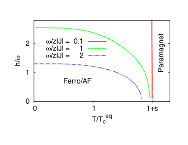
Figure 2: Non-equilibrium phase diagram in the drive vs temperature plane for different values of $\omega$ given in the key. ($s=1$).

Note that $\varphi$ in Eq. (14) must vanish continuously when crossing a second-order phase transition. For a bath with a sub-Ohmic low-energy behavior, $-1\leq s<0$, this implies that the corresponding critical temperature, $T_{{\rm c}}$, is identical to the equilibrium case: $T_{{\rm c}}=T_{{\rm c}}^{{\rm eq}}$. Thereafter, unless stated otherwise, we shall focus on baths with a super-Ohmic low-energy behavior, $s>0$. In this case, the critical temperature is the non-trivial solution of $T_{{\rm c}}=\pm{\rm sgn}(J)\,[A/B(T_{{\rm c}})]\;T_{{\rm c}}^{{\rm eq}}$. Before solving explicitly for $T_{{\rm c}}$, one can already remark that $T_{{\rm c}}$ must be larger than $T_{{\rm c}}^{{\rm eq}}$ so that the numerator and denominator of Eq. (14) have the same sign for $T_{{\rm c}}^{{\rm eq}}<T<T_{{\rm c}}$, ensuring a well-defined non-zero magnetization solution in that temperature range. Let us now solve for $T_{{\rm c}}$ by considering the case when $h\ll\omega$, for which only the $n=1$ mode contributes significantly (because of the stronger power decay of the Bessel functions for larger $n$’s). In this case, the critical temperature $T_{{\rm c}}$ is determined by

$$\tanh\left(\frac{\omega}{2\,T_{{\rm c}}}\right)=\pm{\rm sgn}(J)\;\frac{1}{2T_{{\rm c}}^{{\rm eq}}}\,\frac{\nu\left(\omega\right)}{\nu^{\,\prime}\left(\omega\right)}.$$ (15)

Note that Eq. (15) has a finite solution only if the norm of the right-hand side is smaller than unity.

Importantly, when $\nu^{\,\prime}(\omega)>0$, the type of order is dictated by the sign of J in the ordinary way: $J>0$ for a ferromagnet, $J<0$ for an anti-ferromagnet. However, it is noteworthy that driving can turn a ferromagnet into an anti-ferromagnet and vice-versa when $\nu^{\,\prime}(\omega)<0$. The choice of sign in Eq. (15) that yields a solution (phase transition) in this case is the opposite of the common Ising model: here when $J>0$, there is an anti-ferromagnetic solution, and when $J<0$, there is a ferromagnetic solution.

Eq. (15) can be solved analytically when the right-hand side of the equation is much smaller than unity, $\nu(\omega)/|\nu^{\prime}(\omega)|\ll T_{{\rm c}}^{{\rm eq}}$, yielding the critical temperature

$$T_{{\rm c}}\approx T_{{\rm c}}^{{\rm eq}}\;\left|\omega\;{\nu^{\,\prime}\left(\omega\right)}\right|/{\nu\left(\omega\right)}\;.$$ (16)

Eq. (16) transparently elucidates that by judiciously choosing the driving frequency or engineering the bath, or both, one can achieve a rather large critical temperatures $T_{{\rm c}}$, much larger than the one for the undriven system, $T_{{\rm c}}^{{\rm eq}}$. To exemplify this point, let us assume that the low-energy energy behavior of the hybridization $\nu(\epsilon)\sim\epsilon^{1+s}$ ($s>0$) holds up to the scale $\omega$. This yields $T_{{\rm c}}\approx(1+s)\,T_{{\rm c}}^{{\rm eq}}>T_{{\rm c}}^{{\rm eq}}$. See also Fig. (1) where we plotted the magnetization as a function of the temperature for different drive strengths. In the temperature range $T_{{\rm c}}^{{\rm eq}}<T<T_{{\rm c}}$, it can be seen from Eq. (14) that the drive is responsible for a finite magnetization on the order of $|\varphi|\sim(h/\omega)^{2/s}\omega/zJ$. In Ref. supp , we show the stability of this non-trivial mean-field solution below $T_{{\rm c}}$. In Fig. (2), we summarized the non-equilibrium phase diagram in the temperature–drive plane by numerically solving for the critical temperatures in all the regimes of $h$ and $\omega$. Beyond the super-Ohmic case, Eq. (15) suggests that one can engineering very high critical temperatures by using the edges of the bath spectrum to realize very large $|\nu^{\prime}(\omega)|$ or by embedding the spins in optical cavities with a finely tunable sharply peaked spectrum.

Equation (14) also readily provides the mean-field critical exponent for the order parameter as function of temperature, $\beta_{T}=1/s$, to be contrasted with the undriven case where the mean-field exponent is $\beta_{T}^{{\rm eq}}=1/2$. This means that, even at the mean-field level, driving changes the nature the phase transition.

Finally, Eq. (14) predicts a diverging magnetization at $T=T_{{\rm c}}^{{\rm eq}}$. Although it was derived under the assumption that $\varphi$ is small, this suggests that the original self-consistency Eq. (10) may have non-trivial solutions $\varphi\neq 0$ which are not connected continuously to $\varphi=0$ and signaling the presence of a first-order phase transition. For example, in the case of baths with a sub-Ohmic low-energy behavior ($-1\leq s<0$), the denominator of Eq. (10) given in Eq. (11b) has $1/(\varphi-\varphi_{n})$ divergences located at every $\varphi_{n}\equiv n\omega/2zJ$ for $n=1\ldots\left\lfloor 2zJ/\omega\right\rfloor$. In turn, this implies the presence of a collection of non-trivial solutions of the self-consistent Eq. (10) close to these $\varphi_{n}$’s. For baths with a super-Ohmic low-energy behavior, the denominator Eq. (11b) is well-behaved and we investigate the possibility of a first-order phase transition by solving Eq. (10) numerically. In Fig. (3), we show the non-equilibrium phase diagram in the $T$–$\omega$ plane for a fixed $h/\omega$. Starting from small drive frequencies, the line of second-order phase transitions reaches a tricritical point located at $(\omega^{*}(h/\omega),T_{{\rm c}}^{*}=T_{{\rm c}}^{{\rm eq}})$ and turns into a line of first-order transitions for larger $\omega$.

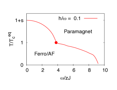
Figure 3: Non-equilibrium phase diagram in the temperature vs drive frequency plane for fixed $h/\omega=0.1$. The red circle indicates the location of the tricritical point separating a second-order line below from a first-order line above. ($s=1$).

Discussion. Besides the demonstration that driven-dissipative conditions can strongly reshape the phase diagram of the Ising model, this study allows us to shine a new light on the fate of the universal properties of this model and, by extension, other similar models when driven to non-equilibrium steady states. When the drive is finite, we have found that the critical exponents (and the critical temperature) are strongly dependent on the details of the bath, thus loosing much of their universality. We hope to report soon on the influence of dimensionality (i.e. away from the mean-field approach) on these results by studying the one-dimensional case via exact methods us .

This work has been supported by the Rutgers CMT fellowship (G.G.), the NSF grant DMR-115181 (C.A.), and the DOE Grant DEF-06ER46316 (C.C.).

Supplementary Material

Stability of the mean-field solutions

Here we check whether the non-zero mean-field solutions in Eq. (14) are stable. We start with a Master Equation for the probabilities $P_{\uparrow}$ and $P_{\downarrow}$ in terms of the rates ${R_{\downarrow\uparrow}}$ and ${R_{\uparrow\downarrow}}$:

$$\dot{{\rm P}}_{\uparrow}= -{R_{\uparrow\downarrow}}\,{P_{\uparrow}}+{R_{\downarrow\uparrow}}\,{P_{\downarrow}}$$

$$\dot{{\rm P}}_{\downarrow}= +{R_{\uparrow\downarrow}}\,{P_{\uparrow}}-{R_{\downarrow\uparrow}}\,{P_{\downarrow}}\;.$$

Using $P_{\uparrow}=(1\pm\varphi)/2$ and $P_{\downarrow}=(1\mp\varphi)/2$ for the ferromagnetic and anti-ferromagnetic cases, respectively, yields

$$\pm\dot{\varphi}= \left[{R_{\downarrow\uparrow}}(\varphi)-{R_{\uparrow\downarrow}}(\varphi)\right]-\left[{R_{\downarrow\uparrow}}(\varphi)+{R_{\uparrow\downarrow}}(\varphi)\right]\;(\pm\varphi)$$

or, equivalently,

$$\dot{\varphi}= -\left[{R_{\downarrow\uparrow}}(\varphi)+{R_{\uparrow\downarrow}}(\varphi)\right]\left\{\varphi\mp\frac{{R_{\downarrow\uparrow}}(\varphi)-{R_{\uparrow\downarrow}}(\varphi)}{{R_{\downarrow\uparrow}}(\varphi)+{R_{\uparrow\downarrow}}(\varphi)}\;\right\}\;.$$

The quantity in curly brackets vanishes at the stationary point, and gives precisely the condition in Eq. (10). Let $\bar{\varphi}$ be this stationary point solution. To consider the stability of fluctuations, we expand $\varphi=\bar{\varphi}+\delta\varphi$. The expansion of the terms in curly brackets start at order $\delta\varphi$ (because $\bar{\varphi}$ is where it vanishes); so to lowest order, the term in square brackets does not need to be expanded. The linearized stability equation becomes

$$\dot{\delta\varphi}= -\left[{R_{\downarrow\uparrow}}(\bar{\varphi})+{R_{\uparrow\downarrow}}(\bar{\varphi})\right][1\mp C(\bar{\varphi})]\;\delta\varphi\;,$$

where

$$C(\bar{\varphi})=\frac{d}{d\varphi}\left(\frac{{R_{\downarrow\uparrow}}(\varphi)-{R_{\uparrow\downarrow}}(\varphi)}{{R_{\downarrow\uparrow}}(\varphi)+{R_{\uparrow\downarrow}}(\varphi)}\right)\Bigg{|}_{\bar{\varphi}}\;.$$

Notice that ${R_{\downarrow\uparrow}}(\bar{\varphi})+{R_{\uparrow\downarrow}}(\bar{\varphi})>0$, so the stability of the solution rests upon whether $[1\mp C(\bar{\varphi})]>0$.

Using Eq. (13), we find

$$1\mp C(\bar{\varphi})= \mp\beta zJ\,\frac{d}{d\varphi}\;\frac{K\,|2zJ\varphi|^{s}+A}{K\,|2zJ\varphi|^{s}+B}\Bigg{|}_{\bar{\varphi}}$$

$$= \mp\beta zJ\,(A-B)\left[\frac{d}{d\varphi}\;\frac{1}{K\,|2zJ\varphi|^{s}+B}\Bigg{|}_{\bar{\varphi}}\right]\;.$$

The quantity in the square bracket above is always negative. Therefore, the sign of $1\mp C(\bar{\varphi})$ is that of $\pm{\rm sgn}(J)\,(A-B)$. Now recall that $T_{{\rm c}}=\pm{\rm sgn}(J)\,[A/B(T_{{\rm c}})]\;T_{{\rm c}}^{{\rm eq}}$ is larger than $T_{{\rm c}}^{{\rm eq}}$ for the non-trivial magnetization to be well defined; therefore $\pm{\rm sgn}(J)\,A>B$. Thus, $\pm{\rm sgn}(J)\,(A-B)>B[1\mp{\rm sgn}(J)]\geq 0$. Hence, we conclude that the sign of $1\mp C(\bar{\varphi})$ is positive and the solutions we found are stable.

References

- (1) A. J. Bray, Adv. Phys. 51, 481 (2002).
- (2) J. J. Arenzon, A. J. Bray, L. F. Cugliandolo, A. Sicilia, Phys. Rev. B 98, 145701 (2008).
- (3) J. Dziarmaga, Phys. Rev. B 74, 064416 (2006).
- (4) A. Sicilia, J. J. Arenzon, Alan J. Bray, L. F. Cugliandolo, EPL 82, 10001 (2008).
- (5) C. Aron, C. Chamon, L. F. Cugliandolo, M. Picco, J. Stat. Mech. P05016 (2008).
- (6) D. W. Hone, R. Ketzmerick, and W. Kohn, Phys. Rev. E 79, 051129 (2009).
- (7) P. A. Rikvold, H. Tomita, S. Miyashita, and S. W. Sides, Phys. Rev. E 49, 5080 (1994).
- (8) R. A. Ramos, P. A. Rikvold, and M. A. Novotny, Phys. Rev. B 59, 9053 (1999).
- (9) F. Berthier, B. Legrand, J. Crueze and R. Tetot, J. Electroanal. Chem. 561, 37 (2004).
- (10) F. Berthier, B. Legrand, J. Creuze and R. Tetot, J. Electroanal. Chem. 562, 127 (2004).
- (11) S. Frank, D. E. Roberts and P. A. Rikvold, J. Chem. Phys. 122, 064705 (2005).
- (12) S. Frank and P. A. Rikvold, Surf. Sci. 600, 2470 (2006).
- (13) B. K. Chakrabarti and M. Acharyya, Rev. Mod. Phys. 71, 847 (1999).
- (14) S. W. Sides, P. A. Rikvold and M. A. Novotny, Phys. Rev. Lett. 81, 834 (1998).
- (15) S. W. Sides, P. A. Rikvold, and M. A. Novotny, Phys. Rev. E 59, 2710 (1999).
- (16) G. Korniss, C. J. White, P. A. Rikvold, and M. A. Novotny, Phys. Rev. E 63, 016120 (2000).
- (17) H. L. Richards, S. W. Sides, M. A. Novotny, and P. A. Rikvold, J. Magn. Magn. Mater. 150, 37 (1995).
- (18) M. A. Novtny, G. Brown, and P. A. Rikvold, J. Appl. Phys. 91, 6908 (2002).
- (19) T. Tome and M. J. de Oliviera, Phys. Rev. A 41, 4251 (1990).
- (20) J. F. F. Mendes and E. J. S. Lage, J. Stat. Phys. 64, 653 (1991).
- (21) M. F. Zimmer, Phys. Rev. E 47, 3950 (1993).
- (22) G. M. Buendia and E. Machado, Phys. Rev. E 58, 1260 (1998).
- (23) M. Acharyya and B. K. Chakrabarti, Phys. Rev. B 52, 6550 (1995).
- (24) B. Chakrabarti and M. Acharyya, Rev. Mod. Phys. 71, 847 (1999).
- (25) W. S. Lo and R. A. Pelcovits, Phys. Rev. A 42, 7471 (1990).
- (26) G. Korniss, P. A. Rivkold and M. A. Novotny, Phys. Rev. E 66, 056127 (2002).
- (27) D. T. Robb, P. A. Rivkold, A. Berger and M. A. Novotny, Phys. Rev. E 76, 021124 (2007).
- (28) H. Fujisaka, H. Tutu and P. A. Rikvold, Phys. Rev. E 63, 036109 (2001); 63, 059903(E) (2001).
- (29) H. Tutu and N. Fujiwara, J. Phys. Soc. Jpn. 73, 2680 (2004).
- (30) E. Z. Meilikhov, JETP Lett. 79, 620 (2004).
- (31) S. B. Dutta, Phys. Rev. E 69, 066115 (2004).
- (32) D. T. Robb, Y. H. Xu, A. Hellwig, J. McCord, A. Berger, M. A. Novotny and P. A. Rivkold, Phys. Rev. B 78, 134422 (2008).
- (33) M. Bukov, L. D’Alessio, A. Polkovnikov, arXiv:1407.4803 (2014).
- (34) L. M. Duan, E. Demler and M. D. Lukin, Phys. Rev. Lett. 91, 090402 (2003).
- (35) M. Greiner, O. Mandel, T. Esslinger, T. W. Hänsch and I. Bloch, Nature 415, 39 (2002).
- (36) M. J. Hartmann, F. G. S. L. Brandao and M. B. Plenio, Laser & Photon. Rev. 2, 527 (2008).
- (37) See Supplementary Material.
- (38) G. Goldstein, C. Aron, T. Iadecola, and C. Chamon, to be published.