Herschel-ATLAS: The Surprising Diversity of Dust- Selected Galaxies in the Local Submillimetre Universe

Abstract

We present the properties of the first 250 µm blind sample of nearby galaxies ($15<D<46\,{\rm Mpc}$) containing 42 objects from the Herschel Astrophysical Terahertz Large Area Survey (H-ATLAS). Herschel’s sensitivity probes the faint end of the dust luminosity function for the first time, spanning a range of stellar mass ($7.4<{M_{\star}}<11.3\ {\rm log_{10}\,M_{\odot}}$), star formation activity ($-11.8<{\it SSFR}<-8.9\ {\rm log_{10}\,yr^{-1}}$), gas fraction (3–96 per cent), and colour (0.6 < FUV-$K_{S}$ < 7.0 mag). The median cold dust temperature is 14.6 K, colder than in the Herschel Reference Survey (18.5 K) and Planck Early Release Compact Source Catalogue (17.7 K). The mean dust-to-stellar mass ratio in our sample is higher than these surveys by factors of 3.7 and 1.8, with a dust mass volume density of $(3.7\pm 0.7)\times 10^{5}\,{\rm M_{\odot}\,Mpc^{-3}}$. Counter-intuitively, we find that the more dust rich a galaxy, the lower its UV attenuation. Over half of our dust-selected sample are very blue in FUV-$K_{S}$ colour, with irregular and/or highly flocculent morphology; these galaxies account for only 6 per cent of the sample’s stellar mass but contain over 35 per cent of the dust mass. They are the most actively star forming galaxies in the sample, with the highest gas fractions and lowest UV attenuation. They also appear to be in an early stage of converting their gas into stars, providing valuable insights into the chemical evolution of young galaxies.

1   Introduction

On average, half of all starlight emitted by galaxies is absorbed by dust and thermally re-emitted in the Far-InfraRed (FIR) and submillimetre (submm) (Fixsen et al., 1996; Driver et al., 2007). Dust is particularly prevalent in star forming regions, where the high-energy photons emitted by young stars are highly susceptible to absorption by dust grains (Fitzpatrick, 2004). The thermal emission from dust in galaxies is normally dominated by the hot component, which is mostly heated by star-forming regions (Kennicutt, 1998; Kennicutt et al., 2009). Thermal emission from dust therefore provides an invaluable avenue for the study of star formation. The cold diffuse dust component dominates the mass of dust in galaxies (Draine et al., 2007; Law et al., 2011; Ford et al., 2013; Hughes et al., 2014), but it is unclear if this cold component is also indirectly heated by star formation through UltraViolet (UV) photons leaking from birth clouds, or if the evolved stellar population is mainly responsible (Bendo et al., 2012; Boquien et al., 2011; Bendo et al., 2014). Ultimately, the ratio of recent/evolved stellar heating is likely to depend on an individual galaxy’s dust geometry and star formation activity (Dunne, 2013). Knowledge of how this ratio depends on measurable properties (e.g. morphological type, $L_{\it TIR}$, colour, etc) would make the determination of star formation rates from FIR measurements more reliable.

The InterStellar Medium (ISM) is enriched by evolved stars, which synthesise heavy elements and then introduce them to the galactic environment. Interstellar dust is now understood to be the product of both winds from evolved stars (Ferrarotti & Gail, 2006; Sargent et al., 2010), and of core-collapse supernovae (SNe), the end-point in the fleeting lives of massive stars (Dunne et al., 2003, 2009; Barlow et al., 2010; Matsuura et al., 2011; Gomez et al., 2012b; Indebetouw et al., 2014). However studies of both local (Matsuura et al., 2009; Dunne et al., 2011) and high-redshift (Morgan & Edmunds, 2003; Dwek et al., 2007; Michałowski et al., 2010; Rowlands et al., 2014b) galaxies have shown a disparity between the rate at which dust is removed from the ISM (either by star formation or interstellar destruction), and the rate at which stars replenish it. As such, the origin of dust in galaxies is still very much an open question.

It is difficult to develop a thorough understanding of galaxies without also understanding the properties of their ISM. As FIR and submm astronomy has matured, numerous projects have been undertaken to characterise dust in galaxies. The galaxy dust mass function was first measured for $\sim$ 200 InfraRed (IR) and optically selected galaxies by the Submillimetre Common-User Bolometer Array (SCUBA) Local Universe Galaxy Survey (SLUGS, Dunne et al., 2000; Vlahakis et al., 2005). This is being followed in the era of the Herschel Space Observatory (Pilbratt et al., 2010) by the Herschel Reference Survey (HRS, Boselli et al., 2010) and the Key Insights in Nearby Galaxies Far-Infrared Survey with Herschel (KINGFISH, Kennicutt et al., 2011). However, these and other FIR surveys of nearby galaxies may have been hindered by the fact they are not dust selected, instead they are selected for their properties at other wavelengths. Large-area missions such as with the Infrared Astronomical Satellite (IRAS, Neugebauer et al. 1984) and more recently Planck (Planck Collaboration et al., 2011a) provide blindly selected FIR/submm samples of local galaxies, including the recent sample by Clemens et al. (2013), but lack resolution and sensitivity when compared to the targeted surveys.

Now, however, with the advent of blind, large-area surveys such as the Herschel Astrophysical Terahertz Large Area Survey (H-ATLAS, Eales et al., 2010) we finally have an unbiased and unrivalled view of the dusty Universe, with resolution and sensitivity hitherto only found in targeted dust surveys.

In this paper, we use H-ATLAS to select local dusty galaxies, and investigate the properties of sources chosen on the basis of their dust mass. In Section 2 we introduce the observations and sample selection. In Section 3 we give an account of our extended-source photometry. In Section 4, we discuss the key properties of our local H-ATLAS sample. In Section 5 we compare the properties of our sample with other samples of nearby dusty galaxies. In Section 6 we examine the gas and dust evolution of the galaxies in our sample. A companion paper on the dust properties of HI-selected galaxies in the local Universe will be presented in De Vis et al. (in prep.). We adopt the cosmology of Planck Collaboration et al. (2013), specifically $\rm H_{0}=67.30\,km\,s^{-1}\,Mpc^{-1}$, $\Omega_{m}=0.315$, and $\Omega_{\Lambda}=0.685$.

2   Herschel Data and the HAPLESS Sample

2.1   Observations

Observations for H-ATLAS were carried out in parallel mode at 100 and 160 µm with the Photodetector Array Camera and Spectrometer (PACS, Poglitsch et al., 2010) and at 250, 350 and 500 µm with the Spectral and Photometric Imaging REceiver (SPIRE, Griffin et al., 2010) instruments on board Herschel. Descriptions of the H-ATLAS data reduction can be found in Ibar et al. (2010) for PACS, and Pascale et al. (2011) and Valiante et al. (in prep.) for SPIRE. Photometry in the SPIRE bands was performed upon maps reduced for extended-source measurements. Our H-ATLAS PACS maps were reduced using the Scanamorphos (Roussel, 2013) pipeline, with appropriate corrections made for the relative areas of the reference pixels on the focal plane.

This work makes use of the H-ATLAS Phase-1 Version-3 internal data release (Valiante et al., in prep., Bourne et al., in prep.), which comprises 161.6  deg² coincident with the Galaxy And Mass Assembly (GAMA, Driver et al., 2009) redshift survey. GAMA provides spectroscopic redshifts, along with supplementary reductions and mosaics of ultraviolet (UV) GALEX (Morrissey et al., 2007; Liske et al., submitted.; Andrae et al., in prep.), optical SDSS DR6 (Adelman-McCarthy et al., 2008), Near-InfraRed (NIR) VISTA VIKING (Sutherland, 2012), and Mid-InfraRed (MIR) WISE (Wright et al., 2010; Cluver et al., 2014) data; details of these reprocessed maps can be found in Driver et al., (in prep.).

Table 1: Basic properties of the HAPLESS sample. Velocities corrected for bulk deviation from Hubble flow (Baldry et al., 2012). Morphologies from EFIGI (Baillard et al., 2011).

HAPLESS	Common name	H-ATLAS IAU ID	SDSS RA	SDSS DEC	$z$	Corrected velocity	Distance	Morphology	Flocculence
			(J2000 deg)	(J2000 deg)	(helio)	(km s-1)	(Mpc)	(T)
1	UGC 06877	HATLAS J115412.1+000812	178.55114	0.13663	0.00379	1336	18.3b	-1	0.25
2	PGC 037392	HATLAS J115504.7+014310	178.77044	1.71981	0.00421	1796	26.7	8	0.75
3	UGC 09215	HATLAS J142327.2+014335	215.86297	1.72630	0.00457	1726	25.6	6	0.75
4	UM 452	HATLAS J114700.5-001737	176.75303	-0.29422	0.00470	1970	29.3	11	0.25
5a	PGC 052652	HATLAS J144430.6+013120	221.12828	1.52201	0.00475	1728	25.7	10	0.25
6	NGC 4030	HATLAS J120023.7-010553	180.09843	-1.10008	0.00477	1978	29.4	3	0.75
7	NGC 5496	HATLAS J141137.7-010928	212.90774	-1.15908	0.00488	1840	27.4	6	0.75
8	UGC 07000	HATLAS J120110.4-011750	180.29502	-1.29751	0.00489	2016	30.0	9	0.50
9	UGC 09299	HATLAS J142934.8-000105	217.39416	-0.01823	0.00516	1904	28.3	9	1.00
10	NGC 5740	HATLAS J144424.3+014046	221.10186	1.67977	0.00520	1890	28.0	3	0.50
11	UGC 07394	HATLAS J122027.6+012812	185.11526	1.46974	0.00526	2197	32.7	7	0.25
12	PGC 051719	HATLAS J142837.8+003311	217.15652	0.55280	0.00527	1952	29.0	7	0.50
13a	LEDA 1241857	HATLAS J145022.9+025729	222.59524	2.95853	0.00533	1928	28.6	10	0.50
14	NGC 5584	HATLAS J142223.4-002313	215.59903	-0.38766	0.00548	2033	22.1b	6	1.00
15a	MGC 0068525	HATLAS J144515.7-000936	221.31587	-0.15953	0.00548	1964	29.2	10	0.25
16	UGC 09348	HATLAS J143228.6+001739	218.11878	0.29402	0.00558	2044	30.4	8	0.50
17	UM 456	HATLAS J115036.2-003406	177.65119	-0.56866	0.00561	2250	33.4	10	0.75
18	NGC 5733	HATLAS J144245.8-002104	220.69130	-0.35108	0.00565	2028	30.1	9	0.75
19	UGC 06780	HATLAS J114850.4-020156	177.21002	-2.03224	0.00569	2261	33.6	8	0.75
20	NGC 5719	HATLAS J144056.2-001906	220.23484	-0.31821	0.00575	2067	30.7	1	0.25
21	NGC 5746	HATLAS J144455.9+015719	221.23300	1.95495	0.00575	2077	30.9	1	0.25
22a	NGC 5738	HATLAS J144356.1+013615	220.98488	1.60418	0.00582	2100	31.2	-2	0.00
23	NGC 5690	HATLAS J143740.9+021729	219.42114	2.29082	0.00583	2130	31.6	3	0.75
24a	UM 456A	HATLAS J115033.8-003213	177.64179	-0.53782	0.00585	2391	31.6	10	0.50
25	NGC 5750	HATLAS J144611.2-001324	221.54635	-0.22294	0.00588	2094	31.1	1	0.25
26	NGC 5705	HATLAS J143949.5-004305	219.95704	-0.71846	0.00591	2097	31.2	9	0.75
27	UGC 09482	HATLAS J144247.1+003942	220.69560	0.66173	0.00607	2177	32.3	8	0.50
28	NGC 5691	HATLAS J143753.3-002354	219.47225	-0.39888	0.00626	2244	33.4	3	0.50
29	NGC 5713	HATLAS J144011.1-001725	220.04794	-0.28897	0.00633	2261	33.6	3	0.50
30	UGC 09470	HATLAS J144148.7+004121	220.45287	0.68697	0.00633	2265	33.6	9	0.75
31	UGC 06903	HATLAS J115536.9+011417	178.90395	1.23717	0.00635	2535	37.7	6	0.75
32	CGCG 019-084	HATLAS J144229.4+013006	220.62338	1.50040	0.00652	2330	34.6	10	0.75
33	UM 491	HATLAS J121953.0+014623	184.97165	1.77347	0.00671	2673	39.7	10	0.50
34	UGC 07531	HATLAS J122611.1-011813	186.54927	-1.30475	0.00675	2654	39.4	9	0.75
35	UGC 07396	HATLAS J122033.9+004719	185.14066	0.78806	0.00706	2779	41.3	8	0.50
36	CGCG 014-014	HATLAS J122106.0+003306	185.27385	0.55283	0.00719	2820	41.9	8	0.25
37	UGC 6879	HATLAS J115425.2-021910	178.60434	-2.31955	0.00803	2774	45.6	4	0.75
38	CGCG 019-003	HATLAS J141919.9+010952	214.83417	1.16516	0.00806	2893	43.0	9	0.50
39	UGC 04684	HATLAS J085640.5+002229	134.16946	0.37500	0.00859	2796	41.5	7	1.00
40	NGC 5725	HATLAS J144058.3+021110	220.24298	2.18626	0.00543	2035	30.2	9	0.75
41a	UGC 06578	HATLAS J113636.7+004901	174.15315	0.81543	0.00375	1164	17.3	10	1.00
42a	MGC 0066574	HATLASJ143959.9-001113	219.99950	-0.18609	0.00620	2246	33.4	11	0.25

• HAPLESS 5, 13, 15, 22, 24, 41, and 42 are not included in the luminosity-limited sub-sample.

• Redshift-independent distances used for HAPLESS 1 (UGC 06877, Tonry et al., 2001), and HAPLESS 14 (NGC 5584, Riess et al., 2011).

The source extraction algorithm used in H-ATLAS (MADX, Maddox et al., in prep., Valiante et al., in prep.) isolates > 2.5 $\sigma$ peaks in the SPIRE 250 µm maps and then measures the fluxes in all three SPIRE bands at the position determined by the 250 µm fit. For our catalogue we further select only those sources which have a > 5 $\sigma$ detection at 250 µm.

Optical counterparts to H-ATLAS sources were found by matching H-ATLAS sources to SDSS DR7 objects (Abazajian et al., 2009) within a 10″ radius using a likelihood ratio technique (Smith et al., 2011). This method uses the optical-submm separation, SPIRE positional errors, and $r$-band magnitudes of potential counterparts, to derive the probability that a given optical galaxy is genuinely associated with the SPIRE source in question (see Smith et al., 2011 and Bourne et al., in prep. for details of the method). Sources with a probability of association $R>0.8$ are deemed to be ‘reliable’ IDs.

2.2   The Sample

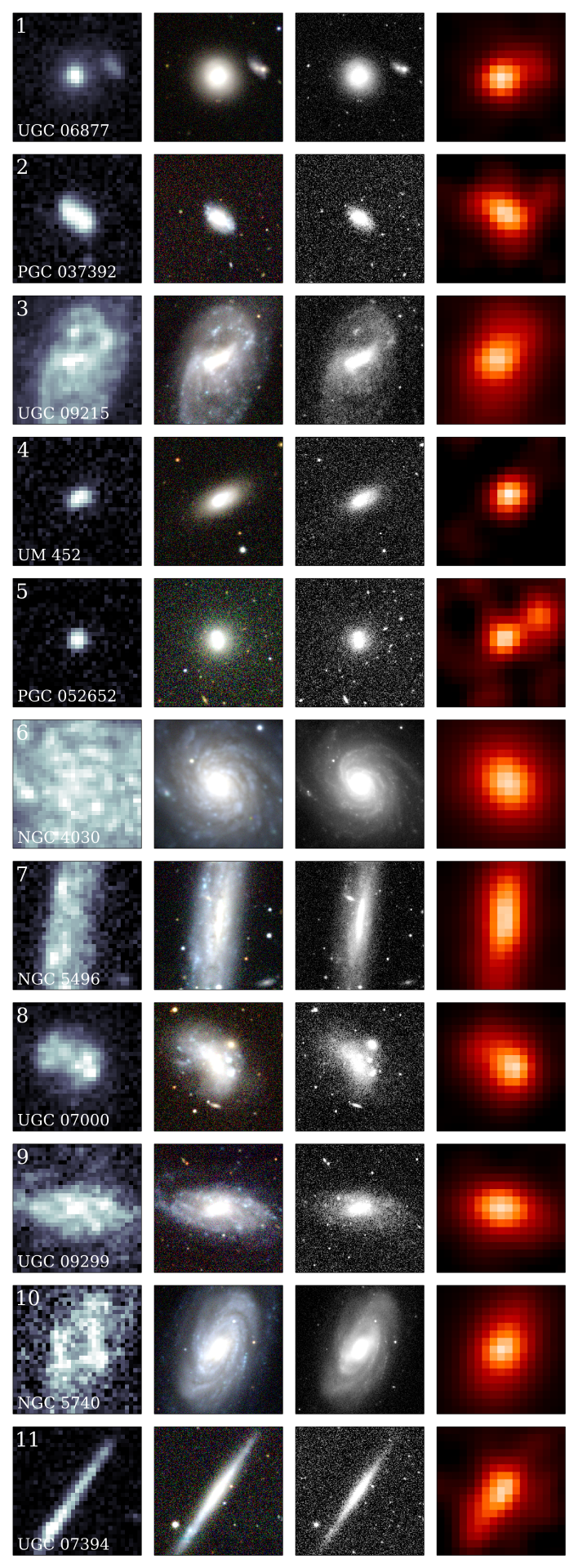
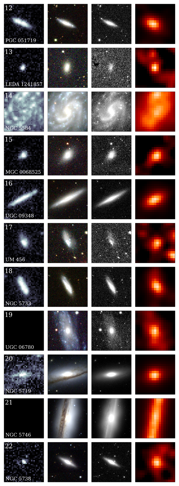
Figure 22: Multiwavelength imagery of each of the HAPLESS galaxies. The bands displayed, from left-to-right, are: GALEX FUV, SDSS gri three-colour, VIKING $K_{S}$-band, and Herschel 250 µm. Each cutout is 100″ on a side. HAPLESS 19 and 21 do not have GALEX coverage.

A sample of 42 galaxies was assembled from the H-ATLAS Phase-1 Version-3 catalogue in the distance range $15<D<46\,{\rm Mpc}$. We wished to sample a volume local enough that we retained sensitivity to the lowest-mass and coldest sources, populations not previously well studied, and our upper distance limit of 46 Mpc serves this purpose well. We do not include galaxies at $D<15\,{\rm Mpc}$, where recessional velocity is no longer a reliable indicator of distance. These galaxies form the Herschel-ATLAS Phase-1 Limited-Extent Spatial Survey, hereafter referred to as HAPLESS. Multiwavelength imagery of the full sample can be found in Appendix A, Figure 22.

We require all sources to have reliable SDSS counterparts ($R\geq 0.8$, Smith et al., 2011) and to have been assessed as having science quality redshifts (nQ $\geq$ 3, Driver et al., 2011) by GAMA. We eyeballed the H-ATLAS maps at the location of all optical sources within the redshift range and found no other candidates which may have been missed by our ID process. The total number of false IDs expected in our sample can be estimated by summing $(1-R)$ (where $R$ is the reliability assigned in the likelihood ratio analysis), which gives a false ID rate of 0.7 per cent.

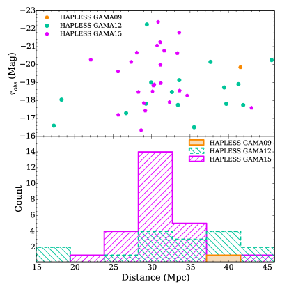
Figure 1: Upper: Absolute r-band magnitude against distance, for the 42 galaxies of the HAPLESS sample. The different colours and shapes denote whether the galaxy lies in the GAMA09 (orange hexagons), GAMA12 (green circles), or GAMA15 (purple pentagons) fields sampled as part of the H-ATLAS Phase 1 data release. Lower: The distance distribution of HAPLESS sources in the different fields.

Distances were calculated using spectroscopic redshifts, velocity corrected by GAMA (Baldry et al., 2012) to account for bulk deviations from Hubble flow (Tonry et al., 2000). For ${\rm H_{0}=67.30\,km\,s^{-1}\,Mpc^{-1}}$, the distance limits we impose correspond to a (flow corrected) redshift range of $0.0035\lesssim z\lesssim 0.01$. Reliable redshift-independent distances were used for the two sources for which they were available; the distance to UGC 06877 has been determined using surface brightness fluctuations (Tonry et al., 2001), and the distance to NGC 5584 is known from measurements of Cepheid variables (Riess et al., 2011).

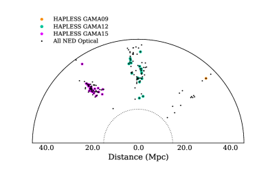
Figure 2: Polar plot of the volume sampled by HAPLESS in the GAMA09, GAMA12, and GAMA15 fields (right-to-left). The positions of the HAPLESS galaxies are shown (same symbols as Figure 1). Also shown are all the optical sources with redshifts that place them in the volume. The inner distance limit of $D=15\,{\rm Mpc}$ is demarked by the dotted black line.

Comparing r-band absolute magnitude (Table 3) to distance, as shown in the upper panel of Figure 1, shows that there appear to be fewer galaxies at greater distances, where larger volumes are being sampled. This is likely to be due to large scale structure (Figure 2), since the percentage cosmic variance on the number counts in the volume sampled by HAPLESS is $\sim 166\,per\,cent$ (Driver & Robotham, 2010). The total number of sources listed in the NASA/IPAC Extragalactic Database (NED) in the same volume as our sample is 141; we therefore detect 30 per cent of this population. Note that the three H-ATLAS fields (GAMA09, GAMA12, and GAMA15; see Figure 1) contain 1, 16, and 25 HAPLESS sources respectively, representing detection rates of 7 per cent, 24 per cent, and 42 per cent.

We identified the portion of our sample which is limited by intrinsic 250 µm luminosity; this gives us a volume limited sample above $L_{250}=8.9\times 10^{21}\,{\rm W\,Hz^{-1}}$ (corresponding to a 250 µm flux of 35 mJy at a distance of 46 Mpc). Of the 42 HAPLESS galaxies, 35 would still be detected were they located at the furthest distance of the volume sampled. Following the assumptions detailed in Section 4.1, this is equivalent to a dust mass limit of $7.4\times 10^{5}\,{\rm M_{\odot}}$ for a dust temperature of 14.6 K (the average dust temperature of the sample, see Section 4.1). The 7 sources fainter than this limit are HAPLESS 5, 13, 15, 22, 24, 41, and 42. These objects are included when describing the properties of our sample in Section 4 and comparing to other surveys in Section 5 but are plotted as hollow circles. We correct for the accessible volume of these sources when considering dust mass volume densities in Section 5.4.

Finally, UGC 06877 (HAPLESS 1) hosts an AGN (Osterbrock & Dahari, 1983), with a significant contribution from non-thermal continuum emission in the UV (Markaryan et al., 1979). This contaminates our star formation rate estimate for this galaxy, rendering it unreliable. We therefore omit HAPLESS 1 from discussions of star formation. The key characteristics of the HAPLESS sample, such as their common names, redshifts, distances and morphologies, can be found in Table 1. We note that 12 of our sources are also part of the smaller nearby sample of H-ATLAS galaxies presented in Bourne et al. (2013).

2.3   Curious Blue Galaxies

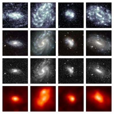
Figure 3: Multiwavelength imagery of four examples of the curious very blue galaxies found in the HAPLESS sample. From left-to-right they are, UGC 09299, NGC 5584, NGC 5733, and NGC 5705. The bands displayed, from top-to-bottom, are: GALEX FUV, SDSS gri three-colour, VIKING $K_{S}$-band, and PSF-filtered Herschel 250 µm. Each image is 150″$\times$ 150″. Note the blue optical colours, flocculent morphologies, NIR faintness, and bright extended UV emission. The whole sample is presented in Appendix A, Figure 22.

We obtained morphology information from the EFIGI catalogue of Baillard et al. (2011), which includes 71 per cent of the HAPLESS galaxies; we visually classified the remainder (all of which were compact dwarf galaxies) using their prescription. The majority of the galaxies in our sample possess very late-type, irregular morphology (Hubble stage $\rm T\geq 8$) though there are two early types (HAPLESS 1 and 22). Furthermore, a large fraction of the sample exhibit a high degree of flocculence (as defined by the EFIGI catalogue). In all, 24 of our sample are classed as irregular, and 19 as highly flocculent; 31 are one or the other, whilst 11 are both (Table 1). These irregular and flocculent galaxies are bright in the submm and UV, indicating significant dust mass and high specific star formation rates (SSFRs). They exhibit extremely blue UV-NIR colours, arising from the fact that, along with being UV-bright, they are NIR-faint; examples of this can be seen in Figure 3. We find a UV-NIR colour-cut of FUV-$K_{S}$ < 3.5 mag to be an effective criterion for identifying such galaxies. This approach is supported by the work of Gil de Paz et al. (2007), who found FUV-$K_{S}$ colour to be a powerful diagnostic for discriminating morphological type.

These curious blue galaxies with FUV-$K_{S}$< 3.5 span a wide range of optical sizes, from 1.3 to 33.3 kpc, with a median major axis of 9.3 kpc (derived from $r$-band $R25$, the radius to the 25^th magnitude square arcsecond isophote). Whilst many of them, particularly the larger examples, possess disks, they often lack defined spiral structure, and show only a weak bulge contribution.

Whilst the FUV-$K_{S}$ colour of UGC 06780 (HAPLESS 1) is 3.07 mag (which would classify it as a member of the curious blue population), continuum emission from its AGN is contributing to the FUV flux. That said, UGC 06780 clearly emits plentiful UV emission not associated with the AGN (especially for an early-type), as it is more extended in the UV than it is in the optical (Table 3). We therefore opt to leave it classed amongst the curious blue population, with this caveat.

GALEX coverage is not available for 2 of the HAPLESS galaxies (HAPLESS 19 and 21); however the colour $u$-$K_{S}$ is well correlated with FUV-$K_{S}$ (Spearman rank correlation coefficient of 0.94 for HAPLESS). By comparing the distributions of these colours, we can state with 3 $\sigma$ confidence that a source with $u$-$K_{S}$< 1.36 will have FUV-$K_{S}$ < 3.5. This indicates that HAPLESS 19 is a member of our curious blue population; visual inspection confirms that it exhibits irregular and extremely flocculent morphology.

The FUV-$K_{S}$ colours of the HAPLESS galaxies can be found in Table 3. Of the 42 HAPLESS galaxies, 27 (64 per cent) satisfy the very blue FUV-$K_{S}$ < 3.5 criterion; 25 (93 per cent) of these exhibit irregular and/or highly flocculent morphology. Of the 15 HAPLESS galaxies with FUV-$K_{S}$ > 3.5, irregular and/or highly flocculent morphology is exhibited by only 7 (47 per cent); a two-sided Fisher test suggests this difference is significant at the $p<0.01$ level.

3   Extended-Source Photometry and Uncertainties

3.1   Extended-Source Photometry

We conducted our own aperture-matched photometry of the HAPLESS galaxies, across the entire UV-to-submm wavelength range, with exceptions for the IRAS 60 µm measurements, and for the PACS 100 and 160 µm aperture fitting; these differences are detailed in Sections 3.1.1 and 3.1.2 respectively. At all other wavelengths, we applied a consistent photometric process, tailored to reliably cope with the wide range of sizes and morphologies exhibited by the sample across the 20 photometric bands employed. These bands are: GALEX FUV and NUV; SDSS ugri, VIKING ZYJHK_s, WISE 3.4, 4.6, 12 and 22 µm; Herschel-PACS 100, and 160 µm; and Herschel-SPIRE 250, 350, and 500 µm. In summary, an elliptical aperture was fitted to a given source in the FUV–22 µm bands. The sizes of these apertures were compared to identify the largest, which was subsequently then used to perform matched photometry across all bands (see Figure 4).

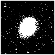
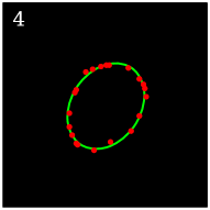
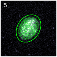
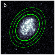
Figure 4: Illustration of the stages of our aperture-fitting process, using GALEX FUV imagery of galaxy NGC 5584 (HAPLESS 14) as an example. Panel 1 shows the inner $500\arcsec\times 500\arcsec$ portion of the cutout centred upon the target source. Panel 2 shows all of the pixels in the cutout with SNR > 3. Panel 3 shows the significant pixels of the target source, contained within their convex hull (red points). Panel 4 shows an ellipse fitted to the convex hull; this ellipse provides the position angle and axial ratio of the source aperture. Panel 5 depicts the incremental annuli used to establish the semi-major axis at which annular flux falls to SNR < 2 (thin concentric lines); 1.2 times this distance is then used as the semi-major axis of the source aperture (thick line). Panel 6 demonstrates the final source aperture (thick line) and sky annulus (thin lines). The apertures at all bands for a given sources are then compared to select the largest, which is then employed for all bands.

In detail, we first cut-out a $2000\arcsec\times 2000\arcsec$ region centred on the target source in each band. In the UV–NIR, bright foreground stars were removed. The SDSS DR9 (Ahn et al., 2012) catalogue was used to identify the locations of the brightest $\sim$ 20 per cent of stars in the field. Locations for stars in non-SDSS bands were also taken from the SDSS catalogue, as it was found to provide the most complete and robust identification of the stars present. Each star was profiled using a curve-of-growth technique, to determine the size of the area to be masked. The pixels in the masked region were then replaced by a random sampling of the pixels immediately adjacent to the edge of the mask.

To provide the position angle and axial ratio of the source aperture, we identified all of the pixels in the cutout that had a SNR > 3 associated with the source, and determined the vertices of their corresponding convex hull. As the vertices of the convex hull trace the outline of the target, least-squares fitting of an ellipse to these points provides the position angle and axial ratio (i.e. the shape, but not the size) of the elliptical source aperture for the band in question.

The semi-major axis of the source aperture was determined by placing successive concentric elliptical annuli (with the already-determined postion angle and axial ratio) on the target, centred on the optical SDSS position, with semi-major axes separated by one pixel-width, until a mean per-pixel SNR < 2 was reached. As flux associated with a source with a Sersic profile will fall beyond the edge of any practical SNR cutoff, the fitted aperture was multiplied by a factor of 1.2, large enough to be confident of encompassing nearly all the flux, whilst small enough to minimise aperture noise. The effects of using different extension factors, tests upon simulated sources, and visual inspection, all indicate that the factor of 1.2 used here achieves this well. This then defined the size of the source aperture. The semi-major and -minor axes of the generated apertures were compared across wave-bands (after subtracting in quadrature the PSF appropriate to that band), and the largest selected as the definitive photometric aperture, to be employed in every band for a given source. GALEX FUV or NUV served as the defining band for most sources, except in the case of early-type galaxies (and the more early-type spirals), for which it was generally VIKING $Z$-band. We also determined the $r$-band $R25$ and FUV $R28$ (the radius to the 25^th and 28^th magnitude per square arcsecond isophotes, respectively) of each galaxy, by interpolating between the mean surface density within annuli of one pixel-width; these values are given in Table 3.

For the FUV–MIR, we subtracted the background using a sky annulus with inner and outer semi-major axes of 1.25 and 1.5 times that of the source aperture. For the PACS and SPIRE data we used a larger inner and outer annulus of 1.5 and 2 times the source aperture, thus ensuring enough pixels were sampled to make a valid estimation of the value of the background. In both cases, the average background value was calculated by taking the iteratively 3$\sigma$-clipped mean of all pixels within the sky annulus.

The photometry from the FUV to $K_{S}$-band was corrected for Galactic extinction in line with the GAMA method described in Adelman-McCarthy et al. (2008).

In the case of NGC 5738 (HAPLESS 22), a dwarf lenticular, emission in the submm and UV is confined to a point source at the centre of the galaxy, as is often seen in early-types (Smith et al., 2012b). The standard aperture, defined by NGC 5738’s much larger optical disc, yields poor-quality photometry in the submm bands due to the aperture containing too much background. We therefore opt to utilise Herschel point-source photometry in the case of this one object. NGC 5738 is unique amongst our sample – in all other cases, sources compact in the UV and submm are compact across the spectrum.

3.1.1   IRAS SCANPI Photometry

For IRAS 60 µm we used the Scan Processing and Integration Tool (SCANPI), following the procedure laid out by Sanders et al. (2003). The SCANPI tool is unable to process non-detections where the estimated background is greater than the measured flux; in those cases we record a flux of 0, with an uncertainty equal to the IRAS 60 µm 1 $\sigma$ sensitivity limit of 58 mJy (Riaz et al., 2006).

3.1.2   Herschel PACS Photometry

In the standard H-ATLAS PACS 100 and 160 µm data reduction (Valiante et al., in prep.), Nebuliser (an algorithm to remove the background emission, Irwin, 2010) was used to flatten the maps after they were run through Scanamorphos (which deals with $1/f$ noise on the maps, Roussel, 2013). For sources with apertures > 2.5′, we used the raw Scanamorphos maps instead, as Nebuliser removes some emission at these scales. Nonetheless, we still find that using the same apertures for PACS as for the other bands results in poor photometry. Flux at 100 and 160 µm tends to be concentrated towards the centres of galaxies, often resulting in a small patch of flux at the centre of a much larger aperture; this can drive up the aperture noise enough that a source with clearly-visible flux can count as a ‘non-detection’. As a result, we define our PACS apertures separately, using the 250 µm maps for each source, as these are reliable indicators of where dust emission is present. Apart from using a different band to define the apertures, PACS photometry otherwise proceeds in the same manner as described in the main part of Section 3.1.

3.1.3   Comparison with GALEX-GAMA Photometry

Given the importance of the UV photometry to this work, and the fact that our apertures in most cases were defined by analysis of surface photometry in the FUV, we have made a detailed comparison of our FUV photometry with the Curve-of-Growth (CoG) FUV photometry provided by the GALEX-GAMA survey (Liske et al., submitted.; Andrae et al., in prep.), which has been extensively used in studies of GAMA galaxies. The comparison was conducted for a subset of 17 HAPLESS galaxies relatively unaffected by shredding in the SDSS-based GAMA input catalogue used by the automated GALEX-GAMA CoG analysis. Our FUV apertures were very similar to those derived by the GALEX-GAMA CoG, while our FUV integrated fluxes were initially found to be systematically higher by $\sim$10 per cent, with a similar degree of scatter. This moderate systematic difference in integrated flux was traced to differences in approach to masking foreground stars in the two methods. The only other detectable difference was the additional random uncertainty ($\sim$10 per cent root-mean-square) being introduced by our use of Swarped images in place of the individual tiles used by GALEX-GAMA. We can conclude that both these independent methods are in acceptable agreement.

3.2   Uncertainties

To estimate aperture noise for a source, we first 3 $\sigma$-clipped the pixel values in a given $2000\arcsec\times 2000\arcsec$ cutout (excluding those pixels within the source aperture). Then random apertures were placed across the cutout (again excluding the location of the source aperture itself). Each random aperture was circular, with the same area as the source aperture, and was background-subtracted in the appropriate manner for each band, as detailed above. The pixel values in each random aperture were inspected; if more than 20 per cent lay beyond the cutout’s calculated 3 $\sigma$ threshold, then that random aperture was rejected. This process was repeated until 100 random apertures had been accepted. We found this clipping technique to be necessary in order to prevent the final aperture noise estimates being too dependant upon the locations of the random apertures; otherwise the presence of bright background sources in the random apertures could cause the aperture noise estimate to vary wildly between repeat calculations on a given cutout. The WISE 3.4 and 4.6 µm maps were found to be particularly vulnerable to this effect, due in part to anomalies in the maps (halos, etc) caused by bright foreground stars.

Once 100 random apertures had been accepted, the flux in each was recorded, and the standard deviation of all 100 fluxes was taken to represent the aperture noise. This method of aperture noise estimation includes the contribution from confusion noise in Herschel bands.

We wanted the uncertainty values of our flux measurements to include not only the background noise and random photometric uncertainty, but also include the uncertainty in our ability to measure the total flux of a galaxy. To that end, we performed two tests. Firstly, we repeated the photometry with an aperture size 20 per cent larger for each source. Ideally, the fluxes obtained using these larger apertures would be identical to those obtained from the normal apertures; the amount of deviation between the two lets us gauge the effectiveness of both our aperture-fitting and our background-subtraction. Secondly, we repeated the photometry, but instead estimated the background using a sigma-clipped median within the sky annulus, instead of a sigma-clipped mean. These should both be equally valid methods, and so the deviation between the final fluxes returned by them allows us to gauge the limits of our ability to accurately determine the background. The additional uncertainty added by these tests is smaller than the instrumental calibration uncertainties (see below), except in the optical bands, where the instrumental calibration uncertainty is very small.

No systematic difference in measured flux was found for either of these tests. For each of the two tests, the associated error value was determined by calculating the root-median-squared deviation across all 42 sources. For each band, these two error values were then added in quadrature to the band’s calibration uncertainty – as given by Morrissey et al. (2007) for GALEX, the SDSS DR9 Data Release Supplement for SDSS, Edge & Sutherland (2013) for VIKING, the WISE All-Sky Data Release Explanatory Supplement for WISE, the PACS Observers’ Manual for PACS, and the SPIRE Observer’s Manual for SPIRE (see also Bendo et al. 2013). This was then added in quadrature to the aperture noise to provide the final photometric uncertainty.

For the IRAS 60 µm photometry acquired separately using SCANPI, the reported flux uncertainty is added in quadrature to a 20 per cent calibration uncertainty (Sauvage, 2011) to provide the total photometric uncertainty for each source.

The final fluxes and uncertainties in all bands can be found in Table 9 in Appendix A.

4   Properties of the HAPLESS Galaxies

4.1   Modified Blackbody SED Fitting

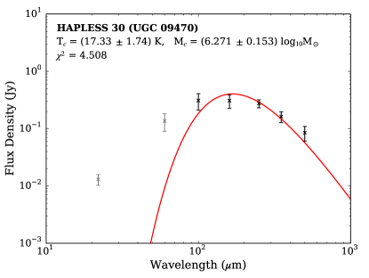
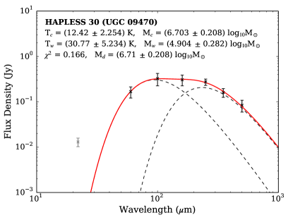
Figure 5: Example dust SED of UGC 09470 (HAPLESS 30), with one- and two-temperature component modified blackbody fits attempted (upper and lower panels respectively). Both used a fixed $\beta=2$. Grey points represent upper limits in the fitting routine. This is an example of a galaxy for which a one-component dust model systematically underestimates the flux at both 100 and 500 µm, whilst overestimating it at 160 µm.

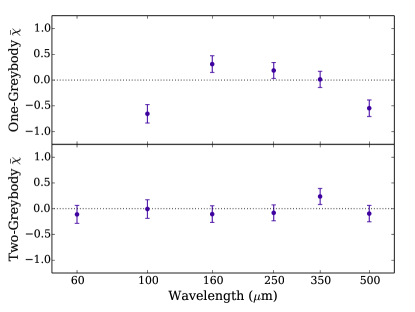
Figure 6: The mean residual across the sample between the model and the data as a fraction of the uncertainty, $\bar{\chi}$, in each band, for the one- and two-temperature modified blackbody fits (example in Figure 5). The single MBB approach systematically overestimates the flux at 160 µm  whilst underestimating it at 100 and 500 µm. The error bars show the uncertainty on the data points, defined by $\sigma=N^{-\frac{1}{2}}$.

To estimate the dust masses and temperatures of the HAPLESS galaxies, we fit Modified BlackBodies (MBBs) of the form $S_{\nu}\propto\nu^{\beta}B(\nu,T_{d})$ to the FIR and submm Spectral Energy Distributions (SEDs), where $\beta$ is the dust emissivity index. We first tried using a single-temperature MBB, keeping $\beta$ fixed at a value of 2 and fitting only those data points with $\lambda\geq 100\,\mu$m. This is because the mid-IR part of the SED has contributions from very small grains which are transiently heated by single photons, and therefore not in equilibrium with the radiation field (Boulanger & Perault, 1988; Desert et al., 1990). This contribution results in a power-law behaviour for the portion of the SED between 12-70 µm and including this data in the single-temperature MBB fit would bias the temperature high. Figure 5 (upper) shows an example of a single-temperature MBB; overall we found that this method systematically underestimated the fluxes at 100 and 500 µm, whilst overestimating them at 160 µm. We demonstrate this using the stacked residuals between the model and the data in Figure 6.

The residuals suggest that a ‘flatter’ SED, produced either by a lower value of $\beta$ or by having dust at a range of temperatures (Dunne & Eales, 2001; Shetty et al., 2009), would be more suitable. We next tried leaving $\beta$ as a free parameter and found a wide range of $\beta$ values (0–4) could adequately fit the HAPLESS sources. Whilst this greatly reduced the systematic bias, it did not eliminate it. Kelly et al. (2012) recently demonstrated that $\chi^{2}$ SED fitting routines with a given ‘true’ value of $\beta$, can return a wide range of fitted values for $\beta$ (see also Smith et al., 2013); furthermore Galametz et al. (2012a) demonstrated that a variable $\beta$ will produce less accurate results than using a fixed value. We therefore use a fixed $\beta$ of 2 in this work, as both observational (Dunne & Eales, 2001; Clemens et al., 2013; Smith et al., 2013; Planck Collaboration et al., 2014) and experimental (Demyk et al., 2013) evidence suggest values between 1.8–2.0 are appropriate for nearby galaxies. Using $\beta=2$ also allows us to easily compare our results to other recent Herschel and Planck studies (see Section 5). A single MBB only provides a useful approximation if the large grains have a narrow range of temperatures (Mattsson et al., in press), which appears not to be the case for many galaxies in HAPLESS (and other FIR surveys; see Mattsson et al., in press, Bendo et al., 2014). We therefore opt to use an SED model which incorporates two temperature components:

$$S_{\nu}=\frac{\kappa_{\nu}}{D^{2}}\left[\ M_{w}B(\nu,T_{w})+M_{c}B(\nu,T_{c})\ \right]$$ (1)

where $S_{\nu}$ is the flux at frequency $\nu$, $\kappa_{\nu}$ is the dust mass absorption coefficient at frequency $\nu$, $M_{w}$ and $M_{c}$ are the hot and cold masses, $B(\nu,T_{h})$ and $B(\nu,T_{c})$ are each the Planck function at frequency $\nu$ and characteristic dust temperatures $T_{h}$ and $T_{c}$, $D$ is the distance to the source. At submm wavelengths, the dust absorption coefficient $\kappa_{\nu}$ varies with frequency as $\kappa_{\nu}\propto\nu^{\beta}$.

We performed the two-temperature MBB fitting from 60–500 µm; the 22 µm point is used as an upper limit to prevent unconstrained warm components from being fitted. A $\chi^{2}$-minimisation routine was used which incorporates colour-corrections for filter response function and beam area. Both temperature components were kept within the 5–200 K range, but were otherwise entirely free. Note that for a galaxy with an SED that is well-fit by a single-component model, this method is free to assign negligible mass to one of the dust components, or fit two identical-temperature components. In keeping with other H-ATLAS works, we use a value for the dust absorption coefficient of $\kappa_{850}=0.077\,{\rm m^{2}\ kg^{-1}}$ from James et al. (2002), which we extrapolate to other wavelengths using a $\beta=2$.

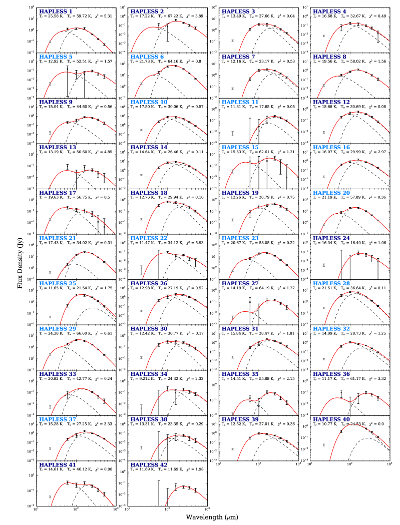
Figure 24: Spectral energy distributions for the HAPLESS sample. The two-temperature modified blackbody fits are shown in red, with the contributions from the warm and cold dust components shown by the dashed curves. The grey 22 µm point was treated as an upper limit. Sources with dark blue names satisfied the FUV-$K_{S}$ < 3.5 colour criterion necessary to be counted amongst the curious blue sub-population; sources with light blue names did not.

Using the two-temperature SED fitting, we no longer encounter any systematic biases in our model fits to the data, as can be seen in the lower panel of Figure 6. Figure 5 shows an example of both one- and two-temperature fits to the SED of HAPLESS 30; the two-temperature fits of all our sources are displayed in Figure 24.

Table 2: Dust properties of the HAPLESS galaxies. Dust masses ($M$) and temperatures ($T$) were derived using a $\chi^{2}$-minimising fit to a two-component modified blackbody SED model, given by Equation 1. Uncertainties were determined by means of a bootstrapping analysis.

HAPLESS	$T_{c}$	$\Delta T_{c}$	$T_{w}$	$\Delta T_{w}$	$M_{c}/M_{w}$	$\Delta M_{c}/M_{w}$	$M_{d}$	$\Delta M_{d}$	$L_{\it TIR}$
	(K)	(K)	(K)	(K)	(log)	(dex)	(log10 M⊙)	(dex)	(log10 L⊙)
1	25.6	1.9	59.7	11.4	2.1	0.8	5.4	0.1	9.0
2	17.2	1.6	67.2	19.3	3.6	1.8	6.0	0.2	8.5
3	13.5	2.4	27.7	2.9	1.3	0.5	7.2	0.2	9.5
4	16.7	4.9	32.7	14.2	1.4	1.3	5.7	0.4	8.4
5	12.9	2.6	52.5	6.8	3.1	1.8	6.0	0.3	8.1
6	21.7	1.0	64.2	16.4	3.2	1.4	7.9	0.1	10.9
7	12.2	2.8	23.2	2.4	1.1	0.6	7.4	0.2	9.5
8	19.6	1.3	58.0	13.8	3.0	1.0	6.4	0.1	9.1
9	15.0	1.6	44.6	12.1	2.9	1.0	6.7	0.2	8.8
10	17.5	2.6	30.1	14.0	1.2	1.0	7.3	0.1	10.0
11	11.3	1.4	17.7	15.6	1.5	2.1	6.9	0.2	8.4
12	15.7	2.4	30.7	9.8	1.5	1.0	6.4	0.2	8.8
13	13.2	3.1	50.6	6.5	2.9	1.6	5.7	0.3	7.9
14	14.6	2.4	26.5	2.9	1.1	0.6	7.4	0.1	9.8
15	15.5	4.3	62.6	9.0	3.4	2.3	5.5	0.5	7.9
16	16.1	3.2	30.0	11.2	1.4	1.1	6.7	0.2	9.2
17	19.6	6.1	56.8	7.9	1.9	1.0	5.3	0.6	8.8
18	12.8	2.5	29.9	3.1	1.5	0.5	6.7	0.2	9.0
19	12.3	1.6	28.8	6.3	2.2	1.1	7.0	0.2	8.8
20	21.2	2.4	57.9	14.2	2.7	1.0	7.5	0.1	10.5
21	17.4	0.9	34.0	18.6	2.5	1.4	8.0	0.1	10.3
22	11.5	2.1	34.1	6.8	1.9	0.7	6.0	0.4	8.1
23	20.7	1.9	58.1	14.8	2.8	1.1	7.6	0.1	10.5
24	16.3	3.9	16.4	4.5	5.7	1.5	5.7	0.3	8.1
25	11.7	1.1	21.5	4.2	0.2	2.2	7.2	0.1	9.6
26	13.0	1.8	27.2	10.2	1.7	1.1	7.4	0.2	9.4
27	14.2	1.6	64.2	5.3	4.3	1.8	6.2	0.2	8.2
28	21.5	4.1	36.6	14.8	1.3	1.1	6.9	0.1	10.1
29	24.4	1.5	66.6	16.8	2.8	1.5	7.6	0.1	10.9
30	12.4	2.4	30.8	3.9	1.8	0.8	6.7	0.3	8.8
31	15.8	3.3	28.5	15.8	1.7	1.5	7.2	0.2	9.5
32	14.1	2.9	28.7	2.5	1.0	0.5	6.6	0.2	9.2
33	20.8	8.2	42.8	13.8	2.1	3.4	5.7	0.8	8.7
34	9.2	2.7	24.3	4.6	1.9	1.0	7.2	0.5	8.6
35	14.5	1.5	55.9	12.3	3.4	0.8	6.7	0.2	8.8
36	11.2	1.1	61.2	18.6	4.1	1.3	6.8	0.2	8.3
37	15.3	2.8	27.3	15.5	1.6	1.4	7.3	0.2	9.5
38	13.3	4.0	23.4	16.0	1.5	2.7	6.2	0.6	8.2
39	12.5	2.9	27.0	2.5	1.2	0.6	7.1	0.3	9.4
40	10.8	6.3	24.5	14.5	0.5	2.3	6.7	0.6	9.2
41	14.6	2.5	46.1	10.9	2.3	0.8	5.8	0.3	8.4
42	11.7	2.5	11.7	14.8	3.2	2.4	6.3	0.4	7.4

Dust masses and temperatures for the HAPLESS galaxies are listed in Table 2. The temperatures of the cold dust components range from 9.2 to 25.6 K, with a median temperature of 14.6 K. The total dust masses range from $2.2\times 10^{5}$ to $9.5\times 10^{7}\,{\rm M}_{\odot}$, with a median mass of $5.6\times 10^{6}\,{\rm M}_{\odot}$. Uncertainties in the derived dust masses and temperatures were estimated by means of a bootstrapping analysis, whereby the fluxes were randomly re-sampled according to a Gaussian distribution defined by the flux uncertainties, and a best fit was made to the re-sampled SED; this was repeated 1,000 times, and the standard deviation in the returned fit parameters was taken to represent their uncertainty. All quoted dust masses are the sum of the cold and warm components, though the cold component significantly dominates the dust mass budget in most of our galaxies (Table 2).

Some galaxies do have SEDs that would be adequately fit by a one-component MBB; in such cases, there is a risk that using the two-component model could give rise to a spurious low-luminosity cold dust component that would yield an artificially large dust mass, and low cold dust temperature. We gauged the potential impact of this effect by weighting the dust temperatures, according to:

$$T_{\it weighted}=\frac{M_{c}T_{c}+M_{w}T_{w}}{M_{c}+M_{w}};$$ (2)

However, this only causes a significant change in temperature for the two galaxies with the lowest values of $M_{c}/M_{w}$ (HAPLESS 25 and 40). The median $T_{\it weighted}$ is only 0.8 K greater than the median $T_{c}$, with no significant difference to any of the trends with temperature reported in this work. It is also important to consider that recent work by Bendo et al. (2014) has shown that low-luminosity cold dust components are present in some galaxies; in such cases, a one-component MBB may be an adequate fit to the data, but not reflect the actual nature of the dust in a galaxy.

It is unclear what relationship the systematic 500 µm excess in our single-temperature MBB fits (Figure 6) bears to the submm excess seen by many other authors (Galliano et al., 2003; Galametz et al., 2012b; Rémy-Ruyer et al., 2013; Ciesla et al., 2014; Grossi et al., 2015) – as we also see an excess at 100 µm, and a deficiency at 160 µm. The two-temperature MBB approach is able to account for all of our systematic residuals without the need for extremely cold ($\ll$ 10 K) dust components.

Total infrared luminosities, $L_{\it TIR}$, from 8–1000 µm were estimated using the best-fit SEDs and extrapolating below 60 µm using a power law to account for the luminosity produced by the transiently heated small grain population. This was done by forcing the SED shape in the mid-IR to a power law, anchored to the WISE 22 µm flux (or the WISE 12 µm flux if this was not available), and the flux at the peak of the best-fit SED (see Ibar et al. 2013 for more details). This new SED was then integrated to produce $L_{\it TIR}$; note that the luminosity using this method was on average 14 per cent higher than simply integrating the best-fit MBBs from 60–500 µm. The values determined using this method are in good agreement with those determined by De Vis et al. (in prep.) derived from performing energy-balance modelling of the full UV–submm SED with MAGPHYS (da Cunha et al., 2008). The resulting $L_{\it TIR}$ values are listed in Table 2.

Table 3: Miscellaneous measured and derived properties of the HAPLESS galaxies. Stellar mass is calculated using Equation 3.

No	$r_{\it abs}$	$R25_{\it r}$	$R28_{{}_{\it FUV}}$	FUV-$K_{S}$	$M_{\star}$
	(Mag)	(arcsec)	(arcsec)	(mag)	(log10 M⊙)
1	-18.0	32	33	3.07a	8.8
2	-17.2	11	17	2.03	8.1
3	-19.6	67	80	2.13	9.2
4	-17.8	21	14	3.16	8.8
5	-17.2	28	13	3.58	8.5
6	-22.2	131	124	4.51	10.8
7	-20.1	124	125	2.66	9.5
8	-19.0	36	37	2.41	9.0
9	-18.4	39	81	1.35	8.6
10	-20.6	89	10	4.39	10.1
11	-18.4	54	56	3.74	8.9
12	-17.8	21	26	3.08	8.6
13	-16.3	13	8	3.14	8.1
14	-20.2	96	92	2.72	9.5
15	-17.4	19	10	3.74	8.6
16	-18.8	43	36	4.26	9.3
17	-17.7	21	21	1.55	8.1
18	-18.5	25	28	2.21	8.7
19	-19.1	102	-	<3.5b	9.2
20	-21.0	115	34	7.00	10.8
21	-22.3	210	-	>3.5b	11.3
22	-18.9	24	34	7.12	9.7
23	-20.7	86	87	4.96	10.2
24	-16.5	10	15	1.82	7.6
25	-21.2	97	51	5.85	10.6
26	-19.9	75	82	2.39	9.5
27	-17.9	37	36	2.90	8.6
28	-20.6	68	39	3.99	9.8
29	-21.7	93	53	4.55	10.4
30	-18.5	33	35	2.24	8.8
31	-20.1	65	74	2.94	9.6
32	-18.2	18	15	3.60	8.9
33	-17.8	13	15	1.58	8.3
34	-18.7	35	15	1.16	8.6
35	-18.9	36	46	2.78	9.0
36	-17.7	21	23	2.32	8.4
37	-20.2	61	56	4.09	10.0
38	-17.5	14	13	2.70	8.4
39	-19.8	36	42	2.34	9.3
40	-18.8	32	29	2.60	8.9
41	-16.5	26	35	0.64	7.6
42	-15.2	4	9	2.47	7.4

• Note that UGC 06877 (HAPLESS 1) is an AGN (Osterbrock & Dahari, 1983), with a contribution from non-thermal continuum emission in the UV (Markaryan et al., 1979).

• Sources UGC 06780 (HAPLESS 19) and NGC 5746 (HAPLESS 21) do not have GALEX coverage. We use the $u$-$K_{s}$ colour to infer whether they belong to the curious blue subset.).

4.2   Stellar Masses

To determine the stellar masses of the HAPLESS galaxies, we follow the method of Zibetti et al. (2009), which assumes a Chabrier (Chabrier, 2003) Initial Mass Function (IMF) and uses $i$-band luminosity along with a relationship between stellar mass-to-light ratio and $g$-$i$ colour. This method combines stellar population synthesis models (Bruzual, 2007) including dust attenuation and compares with a sample of nearby galaxies. Stellar masses arrived at by this method have a typical uncertainty of 0.1–0.15 dex (Cortese et al., 2012b) modulo uncertainties in the underlying population models. Zibetti et al. (2009) caution that their approach may not be appropriate where galaxies have very young stellar populations (where $i$ would be overestimated) or significant extinction (where $i$ would be underestimated); ie, sources with obvious dust lanes (only seen in 6 of the HAPLESS galaxies, Figure 22). As discussed succinctly in Taylor et al. (2011), however, variations in extinction (for simple dust geometries), the star formation history, metallicity and age only serve to shift galaxies along the $(g-i)$ vs $M_{\star}/L_{i}$ relationship, such that uncertainties in these parameters do not produce large errors in the value of stellar mass inferred in this way.

The full formula we employ to calculate stellar mass is:

$$M_{\star}=L_{i}10^{-0.963+1.032(g-i)}$$ (3)

where $M_{\star}$ is stellar mass and $L_{i}$ is $i$-band luminosity, both in Solar units. Stellar masses are listed in Table 3.

The stellar masses of the HAPLESS galaxies range from $2.6\times 10^{7}$ to $2.2\times 10^{11}\,{\rm M}_{\odot}$, with a median mass of $9.8\times 10^{8}\,{\rm M}_{\odot}$. The Zibetti et al. (2009) method yields stellar masses for our sources in excellent agreement with those produced by the more sophisticated MAGPHYS tool which has the ability to model more extincted or highly star-forming systems (De Vis et al., in prep.), and are also in agreement with the masses derived by GAMA (Taylor et al., 2011). We continue to use the colour method in this work in order to compare with other nearby FIR surveys (Section 5).

4.3   Atomic Gas Masses

We searched the literature for the highest-resolution 21 cm observations available for each of the HAPLESS galaxies. We found 15 of our sample have observations in the literature; the instrument and reference for each can be found in Table 4. For the remaining sources, we inspected the Hi Parkes All-Sky Survey (HIPASS, Meyer et al., 2004; Zwaan et al., 2004; Wong et al., 2006) catalogue to find HIPASS sources within the full-width half-maximum (FWHM) of the Parkes beam (14.3′) centred on the positions of the HAPLESS galaxies. To avoid the risk of contamination due to confusion, we only accepted matches for which there were no other known galaxies within 14.3′ radius on the sky, nor within 500 km s^-1 in velocity. This ensures that the matches we accept are isolated in Hi. From HIPASS we identify 16 additional 21 cm detections associated with HAPLESS galaxies.

Table 4: Hi properties of the HAPLESS galaxies. The origin column indicates whether 21 cm data comes from the HIPASS or ALFALFA catalogues, or published literature values. The Hi centroid velocity $V_{R}$ and linewidth $W_{50}$ are not available for all sources with 21 cm measurements. Hi masses were calculated using Equation 4, and gas fraction $f_{g}^{\it HI}$ is defined by Equation 6. Upper limits on the gas mass and gas fraction were derived using Equation 5.

HAPLESS	$S_{\it int}$	$V_{R}$	$W_{50}$	Telescope	Origin	$M_{\it HI}$	$f_{g}^{\it HI}$
	(Jy km s-1)	(km s-1)	(km s-1)			(log10 M⊙)
1	1.30	1146	78	GBT 91 m	Courtois et al. (2011)	8.08	0.13
2	1.39	1308	-	Arecibo	Salzer (1992)	8.36	0.60
3	23.70	1387	222	Parkes	HIPASS	9.56	0.67
4	0.86	1439	140	VLA-D	Taylor et al. (1995)	8.24	0.22
5	0.44	-	-	Arecibo	Impey et al. (2001)	7.83	0.18
6	72.00	1462	306	Parkes	HIPASS	10.16	0.19
7	60.90	1539	243	Parkes	HIPASS	10.03	0.74
8	5.70	-	-	Arecibo	Sulentic & Arp (1983)	9.08	0.52
9	46.90	1537	198	Parkes	HIPASS	9.94	0.96
10	35.80	1528	287	WRST	Popping & Braun (2011)	9.82	0.31
11	5.90	1624	187	Parkes	HIPASS	9.17	0.62
12	3.97	1560	176	Arecibo	ALFALFA	8.90	0.66
13	0.38	1713	26	Arecibo	ALFALFA	7.87	0.37
14	27.10	1638	198	Parkes	HIPASS	9.76	0.47
15	1.08	1652	72	Arecibo	ALFALFAa	8.34	0.35
16	4.26	1673	205	Arecibo	ALFALFA	8.97	0.32
17	3.50	1749	120	VLA-D	Taylor et al. (1995)	8.96	0.88
18	-	-	-	-	-	$<$ 8.67	$<$ 0.45
19	26.90	1729	225	Parkes	HIPASS	9.85	0.82
20	43.50	1736	431	GBT 300 ft	Davis & Seaquist (1983)	9.98	0.12
21	30.70	1724	556	WRST	Popping & Braun (2011)	9.83	0.03
22	-	-	-	-	-	$<$ 8.70	$<$ 0.09
23	25.60	1748	294	Parkes	HIPASS	9.78	0.28
24	2.89	1859	100	VLA-D	Taylor et al. (1995)	8.93	0.95
25	5.30	-	-	Parkes	Bottinelli et al. (1990)	9.08	0.03
26	27.90	1760	184	Parkes	HIPASS	9.80	0.66
27	8.40	1836	224	Parkes	HIPASS	9.31	0.83
28	5.50	1878	150	Parkes	HIPASS	9.16	0.17
29	44.50	1897	317	GBT 300 ft	Davis & Seaquist (1983)	10.07	0.28
30	3.80	-	-	NED	NEDb	9.00	0.62
31	13.30	1891	177	Parkes	HIPASS	9.64	0.51
32	1.81	1916	113	Arecibo	ALFALFA	8.71	0.39
33	6.10	1973	60	VLA-D	Taylor et al. (1995)	9.35	0.91
34	6.50	2033	99	Parkes	HIPASS	9.37	0.86
35	3.22	-	-	Arecibo	Schneider et al. (1990)	9.11	0.52
36	2.04	2143	98	Arecibo	ALFALFA	8.93	0.77
37	-	-	-	-	-	$<$ 9.03	$<$ 0.09
38	1.41	2433	127	Arecibo	ALFALFA	8.79	0.71
39	8.80	2510	148	Parkes	HIPASS	9.55	0.60
40	3.40	1622	148	Parkes	HIPASS	8.87	0.43
41	6.40	1098	124	Parkes	HIPASS	8.65	0.90
42	-	-	-	-	-	$<$ 8.76	$<$ 0.96

• Classified by ALFALFA as a low SNR source (SNR = 5).

• A 21 cm $S_{\it int}$ value for HAPLESS 30 (UGC 09470) is available on NED, but no reference is provided. Despite this, the corresponding Hi properties of HAPLESS 30 are typical of the HAPLESS sample, thus we opt to include it.

For the 11 sources with neither HIPASS nor literature Hi detections available, Hi data for 7 were provided by the ALFALFA (Arecibo Legacy Fast ALFA, Giovanelli et al., 2005) survey (Haynes, priv. comm.). In total we therefore have Hi measurements for 38 (90 per cent) of the objects in our sample.

To calculate our Hi masses, we used the standard prescription:

$$M_{\it HI}=2.36\times 10^{5}S_{\it int}D^{2}$$ (4)

where $M_{\it HI}$ is the mass of atomic hydrogen in Solar units, $S_{\it int}$ is the integrated 21 cm line flux density in Jy km s^-1, and $D$ is the source distance in Mpc.

The Hi properties for each source are listed in Table 4, the atomic gas masses range from $6.8\times 10^{7}$ to $1.5\times 10^{10}\,{\rm M}_{\odot}$, with a median mass of $2.3\times 10^{9}\,{\rm M}_{\odot}$.

The remaining sources fall below the HIPASS detection limit, which typically spans the range $1.6\times 10^{8}<M_{\it HI}<9.8\times 10^{8})\,{\rm M_{\odot}}$ for the distance range of our sample (Haynes et al., 2011). We determine a 3 $\sigma$ upper limit on the Hi mass on our undetected sources using the following prescription from Stevens et al. (2004):

$$M_{\it HI}\leq 2.36\times 10^{5}D^{2}(3\sigma)\sqrt{18}\sqrt{W_{50}}$$ (5)

where $\sigma$ is the RMS noise in a single channel (0.013 Jy), $D$ is the distance in Mpc, the $\sqrt{18}$ accounts for the number of uncorrelated channels (the velocity resolution of HIPASS is $\rm 18\,km\,s^{-1}$), and $W_{50}$ is the linewidth measured at 50 per cent peak intensity. We use the average value of $W_{50}$ observed for the HIPASS-detected HAPLESS galaxies to estimate the upper limits on the Hi mass (Table 4).

To quantify how gas-rich a galaxy is, we calculate the atomic gas fraction $f_{g}^{\it HI}$ for galaxies with detected Hi masses (with upper limits quoted for non-detections); this is defined as:

$$f_{g}^{\it HI}=\frac{M_{\it HI}}{M_{\it HI}+M_{\star}}$$ (6)

where $f_{g}^{\it HI}$ provides a lower limit on the fraction of the baryonic mass in the gas phase (as molecular gas is not considered in this work).

If there is sufficient optical depth in the line of sight for Hi clouds, the Hi fluxes and masses could be under-estimated due to self-absorption. Bourne et al. (2013) show this correction is on average a factor of 1.08 for the overlapping sample of galaxies between their sources and HAPLESS. As we lack the necessary information to calculate the self-absorption for other nearby galaxy surveys (see Section 5.1), we do not consider self-absorption here, but note that our gas masses, particularly for edge on galaxies, could therefore be underestimated by this effect.

Finally, we do not include the molecular gas component in this work due to the lack of uniform measurements for this sample. Since the molecular component only tends to dominate the gas budget in more-massive, earlier-type spirals (Saintonge et al., 2011), our lack of molecular gas information is unlikely to make a substantial difference to the interpretation in this work. Using the scaling relations for $\rm H_{2}$/Hi and stellar mass from Bothwell et al. (2014), the molecular-to-atomic gas ratios in our sample are predicted to be negligible ($<0.1$) for all but 10 of our sources, with the remaining galaxies having ratios between 0.1–0.7. The predicted $\rm H_{2}$/Hi ratios for our curious blue galaxies range from 0.016–0.14 with a median of 0.06 – suggesting using the atomic gas only is an appropriate estimate of the total gas component for these sources. Note that adding molecular gas would only serve to increase the gas fractions in Table 4. The gas masses and gas fractions for the detected galaxies in our sample will be discussed in more detail in Section 5.6.

4.4   Star Formation Rates

To estimate star formation rate (SFR), we use the Hirashita et al. (2003) method of combining UV and IR tracers, specifically following Jarrett et al. (2013) to combine GALEX FUV and WISE 22 µm measurements to give the total SFR as:

$${\it SFR}={\it SFR}_{\it FUV}+{\it SFR}_{22}$$ (7)

where ${\it SFR}_{\it FUV}$ is the FUV-derived unobscured SFR (calculated using Equation 8), and ${\it SFR}_{22}$ is the 22 µm-derived obscured SFR (calculated using Equation 9). All SFR values are in units of ${\rm M_{\odot}\ yr}^{-1}$.

UV emission traces unobscured high-mass stars, indicating star formation on timescales of $\sim$ 100 Myr (Kennicutt, 1998; Calzetti et al., 2005). For ${\it SFR}_{\it FUV}$, we use the prescription of Buat et al. (2008, 2011):

$${\it SFR}_{\it FUV}=10^{-9.69}\nu_{\it FUV}L_{\it FUV}$$ (8)

where $\nu_{\it FUV}L_{\it FUV}$ is the $\nu L_{\nu}$ luminosity in the GALEX FUV waveband in units of bolometric Solar luminosity. Buat et al. (2012) find the uncertainty in this relation to be 0.13 dex. It was calibrated using 656 local galaxies (described in Buat et al. 2007) with stellar masses greater than $10^{10}\,{\rm M_{\odot}}$, and extends down to SFRs of $0.07\,{\rm M_{\odot}\,yr^{-1}}$; as such it includes a range of actively star-forming and quiescent systems. The stellar masses of our sample extend to lower values than the Buat et al. (2007) sample; however the Buat et al. (2007) sample does cover the full luminosity, SSFR, and colour range (specifically NUV-$r$ against FUV-NUV) exhibited by the HAPLESS galaxies. Note that their SFR prescription assumes a Kroupa (2001) IMF; we convert it to the Chabrier IMF (which we use to derive stellar masses) using a correction factor of 0.94.

MIR emission comes primarily from hot dust, heated by short-wavelength photons emitted from newborn stars, and traces star formation on time scales < 100 Myr (Calzetti et al., 2005; Kennicutt & Evans, 2012). The WISE 22 µm SFR relation of Jarrett et al. (2013) was calibrated by bootstrapping to the Spitzer 24 µm SFR relation of Rieke et al. (2009), and is given by:

$${\it SFR}_{22}=(1-\eta)10^{-9.125}\nu_{22}L_{22}$$ (9)

where $\eta$ is the fraction of MIR emission originating from dust heated by the evolved stellar population, and $\nu_{22}L_{22}$ is the $\nu L_{\nu}$ luminosity in the WISE 22 µm waveband in units of bolometric Solar luminosity. Rieke et al. (2009) estimate the uncertainty in their Spitzer 24 µm SFR relation to be 0.25 dex, and find it to be accurate at gauging the star formation giving rise to thermal dust emission in IR-selected galaxies. Jarrett et al. (2013) find the scatter in their WISE 22 µm bootstrap to this relation to be negligible ($\sim$1 per cent), thanks to the close similarity between the Spitzer 24 µm and WISE 22 µm passbands.

The value of $\eta$ will vary from galaxy to galaxy depending on its current star formation activity and dust geometry. $\eta$ may be calibrated independently if other tracers of dust-corrected SFR are available, or calculated theoretically; values in the literature for star forming samples range from $0.17\leq\eta\leq 0.55$ (Buat et al., 2011; Hao et al., 2011; Smith et al., 2012a; Kennicutt & Evans, 2012).

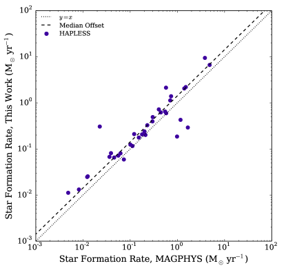
Figure 7: The SFRs calculated using Equation 7 compared to those derived by De Vis et al. (in prep.) by fitting the full UV-submm SEDs of our sample using MAGPHYS da Cunha et al. (2008). The offset between the two prescriptions is by a factor of 1.42, as indicated by the dashed line.

We first set $\eta=0.17$ to be consistent with Buat et al. 2011, and compare our total SFRs using Equation 7 with those derived from SED modelling using MAGPHYS (da Cunha et al. 2008, De Vis et al. in prep.). These two techniques produce SFRs offset by a median factor of 1.42 (see Figure 7). The likely cause is that $\eta=0.17$ is not an accurate measure of the fraction of 22 µm luminosity powered by the older stellar population for our sample, whereas MAGPHYS allows this fraction to be determined by the energy balance between the UV and FIR for each source individually. There may also be differences in the prescriptions for ${\it SFR}_{\it FUV}$ between Buat et al. (2011) and the stellar population models of MAGPHYS (taken from Bruzual & Charlot, 2003; Bruzual, 2007). Finally, the offset could be explained if a bias existed towards a larger transiently-heated small grain population in our sample compared to the Rieke et al. (2009) calibration data (indeed there is some evidence that the 22 µm emission is not correlated with SFR in some H-ATLAS galaxies, Bourne et al. 2013). Modulo the offset, the correlation between the two SFR estimates is tight, with the exception of 4 outliers. The 3 galaxies below the scatter are HAPLESS 9, 33, and 34; these sources have extremely blue FUV-$K_{S}$ colours (< 2.0), and SFRs which are significantly dominated by the unobscured, UV component. The outlier well above the line (HAPLESS 25) is at the extreme red end (in terms of FUV-$K_{S}$) of our sample, and has roughly equal contributions from UV and 22 µm emission to its SFR using Equation 7. The SFR prescriptions therefore appear to disagree in these extreme regions of the parameter space, though we leave this for a future study (De Vis et al., in prep). In order to compare our sources with other nearby galaxy studies, including the HRS (for which we do not have full multiwavelength data) and the Planck sample of Clemens et al. (2013) which uses MAGPHYS (see Section 5) we therefore reduce our SFRs from Equation 7 by a factor of 1.42 to be consistent. Note that this rescaling factor is well within the usual variation found between different SFR prescriptions.

Table 5: Star formation properties of the HAPLESS galaxies. GALEX FUV (unobscured) and WISE 22 µm (obscured) star formation rates, ${\it SFR}_{\it FUV}$ and ${\it SFR}_{22}$, are calculated according to Equations 8 and 9. Where both GALEX and WISE data exists, we combine this (Equation 7) to yield the total SFR.

No	${\it SFR}_{\it FUV}$	${\it SFR}_{22}$	${\it SFR}$	${\it SSFR}$
	(log10 M⊙ yr-1)			(log10 yr-1)
1	-a	-1.2	-	-
2	-1.3	-	-	-
3	-0.4	-0.8	-0.2	-9.5
4	-1.4	-1.9	-1.3	-10.1
5	-1.9	-2.3	-1.7	-10.2
6	-0.0	0.4	0.7	-10.1
7	-0.4	-1.0	-0.3	-9.9
8	-0.7	-1.4	-0.6	-9.6
9	-0.7	-1.6	-0.6	-9.3
10	-0.6	-0.3	-0.0	-10.2
11	-1.4	-1.8	-1.2	-10.1
12	-1.3	-1.8	-1.2	-9.8
13	-2.0	-2.8	-2.0	-10.1
14	-0.3	-0.5	-0.1	-9.6
15	-1.9	-2.2	-1.7	-10.4
16	-1.3	-1.4	-1.0	-10.3
17	-1.0	-1.4	-0.8	-8.9
18	-0.8	-1.4	-0.7	-9.5
19	-	-1.4	-	-
20	-1.3	0.0	0.2	-10.6
21	-	-0.1	-	-
22	-2.3	-2.5	-2.0	-11.8
23	-0.7	0.0	0.2	-9.9
24	-1.4	-2.0	-1.3	-9.0
25	-0.9	-1.0	-0.6	-11.2
26	-0.4	-1.2	-0.3	-9.8
27	-1.4	-2.0	-1.3	-9.9
28	-0.6	-0.2	0.0	-9.8
29	-0.3	0.6	0.8	-9.6
30	-0.9	-1.6	-0.8	-9.6
31	-0.4	-1.1	-0.3	-9.9
32	-1.4	-1.4	-1.0	-9.9
33	-0.9	-1.8	-0.8	-9.2
34	-0.5	-1.9	-0.5	-9.1
35	-0.9	-1.8	-0.9	-9.9
36	-1.3	-	-	-
37	-0.7	-1.1	-0.5	-10.6
38	-1.3	-2.0	-1.2	-9.6
39	-0.5	-1.2	-0.4	-9.8
40	-0.8	-1.4	-0.7	-9.7
41	-1.4	-1.6	-1.1	-8.8
42	-2.3	-	-	-

• Note that HAPLESS 1 has contamination from non-thermal continuum emission in the UV; therefore we do not quote a value for $SFR_{\it FUV}$.

Adding in quadrature the uncertainties in the UV (0.13 dex) and MIR (0.25 dex) relations in Equation 7 yields an uncertainty of 0.28 dex in the derived total SFRs (this does not include the uncertainty in the FUV and 22 µm luminosities of individual sources).

We also calculate the specific star formation rate (SSFR), the SFR per stellar mass (Table 5). The calculated SFRs range from 0.01 to 7.12$\,{\rm M_{\odot}yr}^{-1}$, with a median SFR of $0.18\,{\rm M_{\odot}yr}^{-1}$. Derived SSFRs range from $1.6\times 10^{-12}$ to $1.4\times 10^{-9}\,{\rm yr}^{-1}$, with a median SSFR of $1.3\times 10^{-10}\,{\rm yr}^{-1}$.

5   Properties in Comparison to Other Dust Surveys of Nearby Galaxies

We now compare HAPLESS to other surveys of dust in local galaxies. In this section, we consider our entire sample; however those galaxies that are not in the luminosity-limited subset of HAPLESS are plotted in figures as hollow circles. Table 6 summarises the median properties of each of the samples, and the results of K-S tests between them.

5.1   The Reference Samples

5.1.1   The Herschel Reference Survey

With its stated objective to be the ‘benchmark study of dust in the nearby universe’, the 323 galaxies of the Herschel Reference Survey (HRS, Boselli et al. 2010) have been observed with resolution and sensitivity unrivalled by any previous FIR survey. The HRS chose $K_{S}$-band brightness as its selection criteria, because it suffers least from extinction and is known to be a good proxy for stellar mass. The velocity range of the HRS ($1050\leq V\leq 1750\ \rm km\ s^{-1}$), with corrections made to account for the velocity dispersion of the galaxies of the Virgo Cluster, corresponds to a distance range of $15\leq D\leq 25\ \rm\,Mpc$ (whereas the HAPLESS distance range is $15\leq D\leq 46\ \rm\,Mpc$).

The apparent magnitude limit of the late type galaxies in HRS is $K_{S}\leq 12$, which equates to an absolute magnitude limit between $K_{S}\leq-17.43$ and $K_{S}\leq-18.54$, depending on the distance of the source between the HRS limits. From this we can ascertain that between 4 and 15 of the 42 HAPLESS galaxies would have been insufficiently luminous in $K_{S}$ to have been included in the HRS. These faint HAPLESS galaxies are low stellar mass systems that tend to have very blue FUV-$K_{S}$ colours; 13 of the missing 15 satisfy our FUV-$K_{S}$ < 3.5 criterion. Galaxies seen by H-ATLAS that are faint in $K_{S}$, but nonetheless dusty, represent an orthogonal population to the HRS, and reveal selection biases imposed on targeted dust surveys that H-ATLAS, with its blind sample, is not susceptible to. Another difference between the samples is that the HRS contains numerous early type galaxies, partly due to the stellar mass selection, and partly due to the extensive overlap (46 per cent) of the HRS sample with the Virgo cluster.

To allow for a direct comparison of HAPLESS to the HRS, we determined dust masses and temperatures for the HRS galaxies ourselves, using our own SED-fitting method (as detailed in Section 4.1) and their published PACS (Cortese et al., 2014), SPIRE (Ciesla et al., 2012), and WISE (Ciesla et al., 2014) photometry, along with IRAS 60 µm data we acquired using SCANPI in the same manner as for the HAPLESS galaxies (described in Section 3.1.1). We likewise calculated $L_{\it TIR}$ values for the HRS using the same method as for HAPLESS.

We note that our dust masses for the HRS galaxies are on average a factor $\sim 2.2$ lower than in Ciesla et al. (2014), consistent with their assumed lower value for $\kappa_{500}=0.1\,\rm{m^{2}\,kg^{-1}}$.

Smith et al. (2012b) also find that the submm emission of two HRS sources, the giant elliptical galaxies M87 and M84, contain significant contamination from their AGN. Therefore, we do not attempt to fit the SEDs of these sources.

For the Hi masses of the HRS galaxies, we used the values published in Boselli et al. (2014). The published stellar masses of the HRS (Cortese et al., 2012b) were calculated in the same way as our own. The UV GALEX and optical SDSS photometry of the HRS is described in Cortese et al. (2012a), whilst their NIR $K_{S}$-band photometry (Boselli et al., 2010) was acquired from the 2-Micron All-Sky Survey (2MASS, Jarrett et al. 2000). To calculate the star formation rates of the HRS galaxies, we employed the same technique as for the HAPLESS galaxies (Section 4.4), for which we used the published HRS WISE and GALEX photometry. As for the HAPLESS galaxies, we obtain morphologies for the HRS from EFIGI (Baillard et al., 2011).

5.1.2   Planck

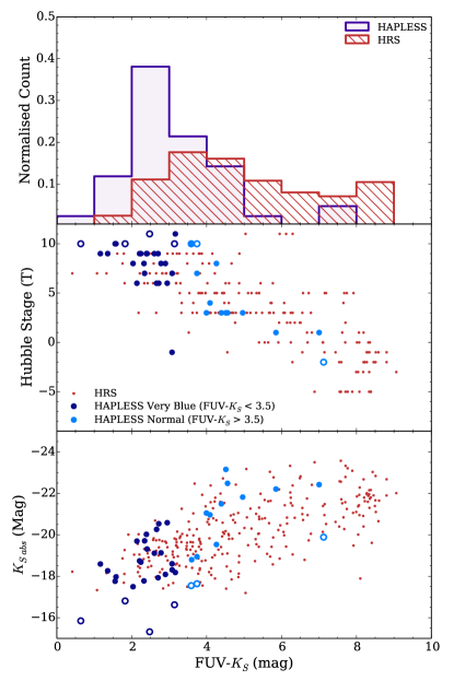
Figure 8: Upper: The distributions of FUV-$K_{S}$ colour for the HAPLESS (blue) and the HRS (red) samples. The galaxies of the blind HAPLESS sample tend to be significantly bluer than those of the $K_{S}$-band selected HRS. Central: Morphology against FUV-$K_{S}$ colour for HAPLESS and the HRS. Lower: Absolute $K_{S}$-band magnitude against FUV-$K_{S}$ colour for HAPLESS and the HRS. Hollow circles indicate galaxies that are below the luminosity-limit of the sample.

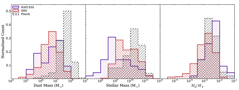
Figure 9: The dust and stellar mass properties of the HAPLESS, HRS, and Planck C13N13 galaxies. Left: The distribution of dust masses. Centre: The distributions of stellar masses. Note that Clemens et al. (2013) derive the stellar masses for the Planck C13N13 sample using MAGPHYS, whilst for the HAPLESS and HRS samples we use Equation 3; however the stellar masses produced by both methods are in excellent agreement with each other for the HAPLESS sample (De Vis et al., in prep.). Right: The distributions of $M_{d}/M_{\star}$ (ie, specific dust mass). HAPLESS contains a much higher proportion of very dust-rich galaxies than either of the other two samples.

Table 6: Median parameters derived for the local-volume surveys compared in this work, including the very blue (FUV-$K_{S}$ < 3.5) subset of the HAPLESS sample. Results from Kolmogorov-Smirnov (K-S) tests between HAPLESS and the HRS and Planck C13N13 surveys are also shown, indicating the likelihood of the null hypothesis that two samples are drawn from the same underlying population.

Sample	FUV-$K_{S}$	$T_{c}$	$M_{d}$	$M_{\star}$	$M_{d}/M_{\star}$	SSFR	$M_{\it HI}$	$M_{d}/M_{\it HI}$	$f_{g}^{\it HI}$	$M_{B}$
	(mag)	(K)	($10^{6}\,\rm{M_{\odot}}$)	($10^{9}\,\rm{M_{\odot}}$)	($10^{-3}$)	($10^{-11}\,\rm{yr^{-1}}$)	($10^{8}\,\rm{M_{\odot}}$)	($10^{-3}$)		($10^{9}\,\rm{M_{\odot}}$)
HAPLESS	2.8	14.6	5.3	1.0	4.4	12.9	14.4a	3.9	0.52	2.5
$\prime\prime$ Very Blue	2.4	14.2	4.8	0.6	6.5	20.7	12.1a	2.7	0.66	2.3
HRS	4.6	18.5	4.6	4.9	1.2	4.1	8.5a	6.2	0.18	5.5
Planck	–	17.7	41.9	17.4	2.5	6.9	36.4a	11.6	0.17	22.4
K-S (HRS)	$10^{-8}$	$10^{-4}$	0.15	$10^{-6}$	$10^{-6}$	$10^{-5}$	$0.03$	$10^{-2}$	$10^{-5}$	$10^{-2}$
K-S (Planck)	–	$10^{-3}$	$10^{-13}$	$10^{-11}$	$10^{-3}$	0.01	$10^{-3}$	$10^{-10}$	$10^{-7}$	$10^{-10}$

• Gas masses are available for 90 per cent of the HAPLESS sample (93 per cent of the very blue subset), 81 per cent of the HRS, and 90 per cent of the Planck C13N13 sample.

Negrello et al. (2013) used the Planck Early Release Compact Source Catalogue (ERCSC) (Planck Collaboration et al., 2011b) to assemble a sample of nearby galaxies. Their flux-limited sample contains 234 dusty galaxies brighter than 1.8 Jy at 550 µm, at distances $\lesssim\,100\,\rm\,Mpc$ (with the vast majority lying at $z<0.01$); the authors estimate the sample to be 80 per cent complete. Clemens et al. (2013) have used this sample to perform a study of the properties of nearby dusty galaxies. We hereafter refer to this as the Planck C13N13 sample.

Whilst the Planck-selected sample benefits from being blind and all-sky (excepting the galactic plane zone of avoidance), Planck suffers from lower sensitivity and resolution compared to Herschel (3.8′ in contrast to 18″). Only 3 of the HAPLESS galaxies exceed the 1.8 Jy 550 µm flux limit necessary to feature in the Planck C13N13 sample (and none of those are members of the curious blue subset).

Clemens et al. (2013) also derived dust masses and temperatures for their sources by fitting two-component MBB SEDs with $\beta=2$, which is consistent with our method. For the Planck C13N13 sample, the authors adopted a value for the dust absorption coefficient of $\kappa_{850}=0.0383\rm{\ m^{2}\ kg^{-1}}$, in contrast to the value in this work of $\kappa_{850}=0.077\rm{\ m^{2}\ kg^{-1}}$. As a result, we have divided their dust masses by a factor of 2.01 to permit comparison.

The Planck C13N13 stellar masses and star formation rates were estimated using the MAGPHYS multiwavelength SED-fitting package (da Cunha et al., 2008), which produces stellar masses which agree exceptionally well with the Zibetti et al. (2009) method we employ (De Vis et al., in prep.); both methods also assume the Chabrier IMF. Hi data were available for 220 (94 per cent) of the Planck C13N13 galaxies Clemens, priv. comm.. Once again, we use EFIGI morphologies (Baillard et al., 2011).

Whilst almost identical sets of observed and derived properties are shared by HAPLESS and the HRS, a more limited set of parameters is available for Planck C13N13; as a result, not all of the following analyses can include the Planck sample.

5.2   Colour and Magnitude Properties

As described in Section 2.3, we find FUV-$K_{S}$ colour to be an effective way of identifying the subset of curious blue galaxies in our sample, using a colour cut of FUV-$K_{S}$ < 3.5. We find that 64 per cent (27) of the HAPLESS galaxies satisfy this criterion, compared to only 27 per cent of the HRS galaxies with FUV-$K_{S}$ colours available. Given that the HRS is $K_{S}$-band-selected, it is to be expected that its galaxies will tend to exhibit redder FUV-$K_{S}$ colour. The distributions of FUV-$K_{S}$ colours for HAPLESS and the HRS are shown in the upper panel of Figure 8. Whilst the HRS more-or-less equally samples a wide range of FUV-$K_{S}$ colours, with a median of 4.6 (Table 6), the blindly-selected HAPLESS galaxies tend to occupy a much narrower range of colours, with a median of 2.8. The distributions are significantly different.

As demonstrated by Gil de Paz et al. (2007), FUV-$K_{S}$ colour is a strong indicator of morphology, as is also seen in the central panel of Figure 8. The very blue FUV-$K_{S}$ colours of the HAPLESS galaxies indicate that the dust-selected universe is dominated by very late type galaxies.

The lower panel of Figure 8 is a colour-magnitude plot constructed using FUV-$K_{S}$ colour and $K_{S}$-band magnitude. Both the blue cloud and red sequence can be seen in the distribution of the HRS, at (3, -19.5) and (8.5, -22); however our HAPLESS sample is skewed towards bluer colours such that the bimodality is not visible in this sample; indeed, many of the HAPLESS galaxies are in fact bluer than the blue cloud peak seen in the HRS distribution.

5.3   Dust and Stellar Mass

Figure 9 compares the dust mass distributions of HAPLESS, HRS, and Planck C13N13. The effect of the 1.8 Jy flux limit at 550 µm in the Planck C13N13 sample is immediately apparent; only galaxies with high dust masses (and a few less massive but very nearby galaxies) were bright enough to be included in their sample, which has a median dust mass of $4.2\times 10^{7}\,{\rm M}_{\odot}$. The HAPLESS and the HRS have different selection effects but ultimately have comparable median dust masses (Table 6).

The three samples also exhibit notably different distributions in stellar mass (Figure 9). The high flux limit of the Planck C13N13 sample naturally biases it towards more massive galaxies. HAPLESS spans the broadest range of stellar masses, but on average has lower stellar mass systems. The median stellar masses of the three samples span over an order of magnitude, and the combination of lower stellar masses, but moderate-to-high dust masses, means the HAPLESS galaxies have the highest median $M_{d}/M_{\star}\sim 4.4\times 10^{-3}$ (ie, specific dust mass) out of the three surveys (Figure 9, Table 6). The very blue subset have an even higher median dust-to-stellar mass ratio of $6.5\times 10^{-3}$; despite accounting for only 6 per cent of the stellar mass in the HAPLESS sample, the curious blue galaxies account for over 35 per cent of the dust mass.

5.4   The Dust Mass Volume Density

We now measure the dust mass function (DMF) and dust mass volume density for HAPLESS. In this analysis, we consider all 42 galaxies in HAPLESS. For the 7 sources that are fainter than the luminosity complete limit, we estimate their accessible volumes using the $1/V_{\it max}$ method (Schmidt, 1968), while for the luminosity complete subset the accessible volume is simply that between the 15–46 Mpc distance limits of the sample ($1,540\,\rm{Mpc^{3}}$).

The upper panel of Figure 10 compares HAPLESS to the dust mass functions of Dunne et al. (2011), Vlahakis et al. (2005), and Clemens et al. (2013). The HAPLESS data points have had the appropriate corrections from Rigby et al. (2011) applied to account for the statistical effects of flux boosting and incompleteness (Section 2.2). The H-ATLAS Science Demonstration Phase (SDP) result for $0<z<0.1$ from Dunne et al. (2011) (orange line in Figure 10) is based on the first 16 square degree field of H-ATLAS. Their dust mass function shown here includes a correction factor of 1.4 for the known under-density of the GAMA09 field at $z$ < 0.1 relative to the average from SDSS (Driver et al., 2011). The Vlahakis et al. (2005) DMF (green line) used submm/IRAS colour relations from the SLUGS survey to estimate 850 µm fluxes, and hence dust masses, for all IRAS galaxies in the PSCz catalogue (Saunders et al., 2000). In order to translate their IRAS plus 850 µm flux estimate to a dust mass they needed to assume a temperature model for the SED, and their cold fit assumes a cold dust temperature of 20 K, which seemed reasonable at the time based on submm studies of IRAS galaxies by Dunne & Eales (2001). The Planck DMF from Clemens et al. (2013) is based on the 550 µm luminosity function from Negrello et al. (2013) and uses the same flux limited sample we have described in Section 5.1.2. Table 7 lists the parameters for the different Schechter functions; we have corrected all DMFs to the same value of $\kappa_{d}$ and the same cosmology used here. We note that uncertainties in the distance measurements of the different galaxy samples could cause considerable scatter in the shape of the DMF, particularly at the high end, as demonstrated by Loveday et al. (1992). This would result in an observed DMF that is effectively a Schechter function convolved with a Gaussian. However, as the distance uncertainties vary both within and between the samples we compare here, we only present the observed mass functions in this work.

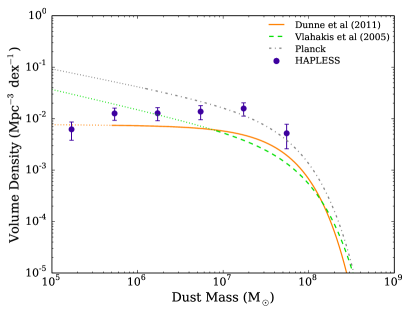
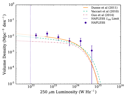
Figure 10: Upper: The HAPLESS dust mass function (with appropriate incompleteness corrections applied) compared with those of Planck C13N13, Vlahakis et al. (2005), and the H-ATLAS Science Demonstration Phase functions from Dunne et al. (2011). Lower: The 250 µm luminosity function of HAPLESS compared with the $z<0.1$ H-ATLAS samples from Dunne et al. (2011), Guo et al. (2014) and the $z<0.2$ sample from HerMES (Vaccari et al., 2010). The error bars on points represent Poisson uncertainty. The functions are plotted as thin dotted lines in the regions where they are extrapolated. All have been adjusted to our $\kappa_{d}$ and cosmology.

Above $M_{d}\sim\,10^{7}\,{\rm M_{\odot}}$, the HAPLESS data points agree with the Planck DMF but are higher than those from Dunne et al. (2011) and Vlahakis et al. (2005). Galaxies with $M_{d}\geq 10^{7}\,\rm{M_{\odot}}$ account for 87 per cent of the total HAPLESS dust mass. Below this mass, the HAPLESS data points are in closer agreement with the Dunne et al. (2011) DMF and directly probe to lower dust masses than any of the previous works. Vlahakis et al. (2005) and Planck C13N13 find a steeper faint-end slope than Dunne et al. (2011) and this work, but their direct sampling of the faint end is 1–2 orders of magnitude less than achieved here. With poor statistics in all surveys at the low-mass end, the varying estimates of the slope agree with each other within their 1 $\sigma$ uncertainties and so we do not consider these differences worrying at present.

Table 7: The best-fit Schecter function parameters of the various dust mass functions and luminosity functions compared in this work. All have been scaled to the same cosmology and value of $\kappa_{d}$ we employ.

Literature Dust Mass Functions
Reference	$\alpha$	$M^{\star}$	$\phi^{\star}$
		(${\rm M_{\odot}}$)	(${\rm Mpc^{-3}\,dex^{-1}}$)
Clemens et al. (2013)	-1.34	$5.27\times 10^{7}$	$11.0\times 10^{-3}$
Dunne et al. (2011)a	-1.01	$4.22\times 10^{7}$	$7.19\times 10^{-3}$
Vlahakis et al. (2005)	-1.39	$6.49\times 10^{7}$	$2.97\times 10^{-3}$
Literature Luminosity Functions
Reference	$\alpha$	$L^{\star}$	$\phi^{\star}$
		(${\rm W\,Hz^{-1}}$)	(${\rm Mpc^{-3}\,dex^{-1}}$)
Dunne et al. (2011)a	-1.14	$1.53\times 10^{24}$	$6.00\times 10^{-3}$
Guo et al. (2014)b	-1.06	$1.12\times 10^{24}$	$3.70\times 10^{-3}$
Vaccari et al. (2010)c	-1.14	$2.19\times 10^{24}$	$4.22\times 10^{-3}$

• Note that this incorporates the 1.42 correction factor applied by Dunne et al. (2011) to account for under density in the GAMA09 field (Driver et al., 2011).

• Guo et al. (2014) use a modified Schechter function to fit their LF, with an additional parameter of $\sigma=0.30$ (explained in Saunders et al., 1990).

• Vaccari et al. (2010) do not provide the parameters to their 250 µm Schechter fit; these values represent our best fit to their quoted data points.

The most significant variation in the dust mass function between HAPLESS and Dunne et al. (2011) is the excess of HAPLESS galaxies around $M_{d}\sim 10^{7}\,\rm{M_{\odot}}$. This could be due to two possible effects: cosmic variance, or incompleteness in the Dunne et al. (2011) DMF.

The volume probed by HAPLESS (and also by the other surveys at the faint end) is very small and subject to a large uncertainty due to cosmic variance ($\sim$ 166 per cent, Section 2.2). This effect can be explored by comparing the 250 µm luminosity functions since this removes the complication of relating the 250 µm emission to the mass of dust. Any differences in the 250 LF will purely be due to variations in the space density of sources in the different samples. We compare HAPLESS to the luminosity functions of previous authors in Table 7 and Figure 10 and find good agreement (within errors) with the $0<z<0.1$ H-ATLAS luminosity function from Dunne et al. (2011) (from 16 ${\rm deg}^{2}$ Science Demonstration Phase data, scaled by their density correction 1.4 factor; this is an updated version of the LF presented in Dye et al. 2010) and from HerMES (over 14.7 ${\rm deg}^{2}$ at $z<0.2$, from Vaccari et al., 2010). The LF derived from H-ATLAS Phase-1 data (161.6 ${\rm deg}^{2}$) in Guo et al. (2014) is lower compared to HAPLESS. This measure has not corrected for the known underdensity of the GAMA09 field and also uses a brighter optical magnitude threshold for inclusion of sources than Dunne et al. (2011). It is not clear how much of a difference this will make (detailed LFs for the full H-ATLAS Phase 1 will be presented in future work) but overall, this comparison indicates that the HAPLESS volume represents a region of fairly typical 250 µm luminosity density and certainly is not significantly overdense relative to the density corrected Dunne et al. (2011) values.

The fact that we find a greater dust mass volume density than Dunne et al. (2011), despite having the same 250 µm luminosity density detection limit, must therefore be ascribed to a difference in the average ratio of $L_{250}/M_{d}$ in the two samples, such that HAPLESS includes dustier objects for a given 250 µm luminosity threshold. The reason behind this lies in the relationship between our selection parameter, $L_{250}$, and our parameter of interest, $M_{d}$. Whether or not we detect a given mass of dust is strongly dependant upon the temperature of that dust. This is illustrated by Figure 11, which compares the relation between 250 µm luminosity and dust mass for HAPLESS and the HRS. The relationship found by Dunne et al. (2011) is shown as a dashed line. There is a scatter of $\sim\,1$ dex in this relationship, due to dust temperature. The HAPLESS galaxies have more dust mass for a given 250 µm luminosity than both the HRS and the Dunne et al. (2011) relation, because they are colder on average than the galaxies in those samples. The issue is therefore that no surveys have a truly ‘dust mass limited sample’ but rather, in the case of H-ATLAS, we have a 250 µm luminosity limited sample. Our luminosity limit of $L_{250}=8.9\times 10^{21}\,{\rm W\,Hz^{-1}}$ for the HAPLESS complete sub-sample translates to an approximate dust mass limit of $7.4\times 10^{5}\,{\rm M_{\odot}}$, using the average HAPLESS dust temperature of 14.6 K. But if we instead use the warmest and coldest temperatures in our sample (10–25 K) this limit becomes ‘fuzzy’ and ranges from $5\times 10^{6}$ to $3\times 10^{5}\,\rm{M_{\odot}}$. We are assuming that a 250 µm luminosity limited sample is equivalent to a dust mass limited sample, when in reality it is not. If we consider the volume accessible to a source with $M_{d}=10^{7}\,{\rm M_{\odot}}$ at a dust temperature of 14 K, compared to that for a source with the same dust mass but at a temperature of 20 K, we find that the warmer source with the same dust mass has an accessible volume 8 times greater than the colder one. The small area in the Dunne et al. (2011) work, combined with this effect, may have resulted in an incompleteness to colder galaxies at the median redshift of sources in the $M_{d}\sim 10^{7}\,{\rm M_{\odot}}$ bins. At the time of the Dunne et al. (2011) work, it was not expected to find many galaxies with such cold dust temperatures. Future work in measuring the dust mass function for the full Phase-1 H-ATLAS area (Dunne et al., in prep.) will address this issue and aim to correct for it.

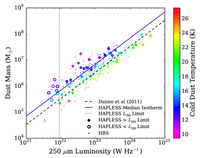
Figure 11: Dust mass against 250 µm luminosity for the HAPLESS and the HRS, colour-coded by cold dust temperature. Also shown are the median dust temperature (solid) for the HAPLESS sources and the relationship in Dunne et al. (2011) (dashed). Filled circles show the HAPLESS luminosity complete sub-sample.

To determine the dust mass density in the HAPLESS volume, we use the combined dust mass of the individual sources, with our luminosity-incomplete sources weighted to account for the fraction of our volume in which they can be detected, according to:

$$\rho_{d}=\frac{\sum{\left(M_{d}\frac{V_{\it tot}}{V_{\it acc}}\right)}}{V_{\it tot}}$$ (10)

where $\rho_{d}$ is the dust mass density, $V_{\it tot}$ is the total sample volume, and $V_{\it acc}$ is the accessible volume for a given source (in the case of the luminosity-complete sources detectable in our entire volume, we treat $V_{\it acc}=V_{\it tot}$). The resulting dust mass density in the HAPLESS volume is $\rho_{d}=(3.7\pm 0.7)\times 10^{5}\,{\rm M_{\odot}\,Mpc^{-3}}$, where the uncertainty includes errors on the dust masses of the individual sources and poisson statistics, but not cosmic variance (in keeping with the errors from other estimates discussed below).

We integrate the Schechter fits to the dust mass functions of Clemens et al. (2013); Dunne et al. (2011) and Vlahakis et al. (2005) down to the average HAPLESS dust mass limit of $7.4\times 10^{5}\,{\rm M_{\odot}}$ to calculate their values of $\rho_{d}$. We account for the difference in $\kappa_{d}$ in the Clemens et al. (2013) work and also note that the units for $\phi^{\star}$ in their Table 2 are actually $\rm{Mpc^{-3}}$ for their own fits and not $\rm{Mpc^{-3}\,dex^{-1}}$ as is written in their paper. The values they quote for $\phi^{\star}$ for Dunne et al. (2011) and Vlahakis et al. (2005) are however in the correct units (Negrello, priv. comm.). We also scale all values to reflect the cosmology used in this work. The corresponding values of the local dust mass volume density are $\rho_{d}=(3.2\pm 0.6)\times 10^{5}\,{\rm M_{\odot}\,Mpc^{-3}}$ for Clemens et al. (2013), $\rho_{d}=(1.3\pm 0.2)\times 10^{5}\,{\rm M_{\odot}\,Mpc^{-3}}$ for Dunne et al. (2011), and $\rho_{d}=1.1\times 10^{5}\,{\rm M_{\odot}\,Mpc^{-3}}$ for Vlahakis et al. (2005). The quoted uncertainty is estimated by retaining the fractional uncertainty of the integrated value quoted in the original works (where applicable). Driver et al. (2007) also estimate the dust mass density from their study of the $B$-band luminosity function assuming a constant ratio of $L_{B}/M_{d}$. They derive a value of $(2.1-2.7\pm 0.8)\times 10^{5}\,{\rm M_{\odot}\,Mpc^{-3}}$, after accounting for our choice of cosmology and the difference in $\kappa_{d}$ used by Driver et al. (2007).

The HAPLESS value of $\rho_{d}=(3.7\pm 0.7)\times 10^{5}\,{\rm M_{\odot}\,Mpc^{-3}}$ is compatible with those of Clemens et al. (2013) and Driver et al. (2007), and is significantly higher than those of Dunne et al. (2011) and Vlahakis et al. (2005). The dust mass density is dominated by sources at and above the knee in the Schechter function, where HAPLESS measures a higher space density than the Dunne et al. (2011) and Vlahakis et al. (2005) surveys. We believe this could be due to incompleteness in the other works in accounting for the very coldest dusty galaxies we see in HAPLESS.

Extrapolation of the DMFs to zero mass suggest that 2–8 percent of dust mass in the local volume is in galaxies below the approximate HAPLESS mass limit, and thus HAPLESS presents a highly complete census (albeit with small statistics at present) of the dust content of the very local universe. Future work exploiting the full H-ATLAS survey, which covers 600 square degrees of sky (compared to the 161.6 square degrees surveyed in this work), will be able to address these matters with far greater statistical power.

5.5   Links Between Star Formation, Colour, and Dust Temperature

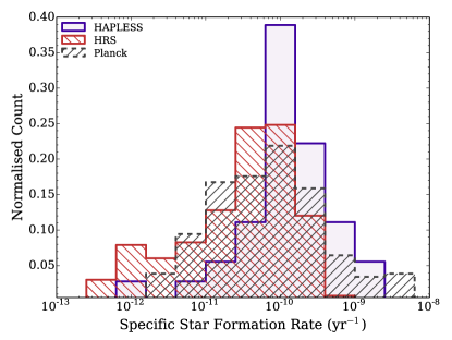
Figure 12: The distribution of SSFRs derived for the HAPLESS, HRS, and Planck C13N13 samples. Whilst the HRS and Planck C13N13 samples show a broad range of SSFRs, the HAPLESS galaxies generally occupy of much narrow range of values, of relatively high SSFRs.

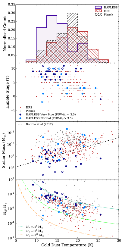
Figure 13: Cold dust temperatures relations for the HAPLESS, HRS, and Planck C13N13 galaxies. From top-to-bottom – 1^st: The distribution of cold dust temperatures. 2^nd: The relation between morphological type and cold dust temperature; HAPLESS is heavily skewed towards cold late-type galaxies. 3^rd: Stellar mass versus cold dust temperature with the relation from Bourne et al. (2012). 4^th: $M_{d}/M_{\star}$ against cold dust temperature. Curves represent different observing limits in $M_{d}/M_{\star}$ due to the cold dust temperature for a given value of $M_{\star}$. Hollow circles indicate galaxies that are beneath the luminosity-limit of the sample.

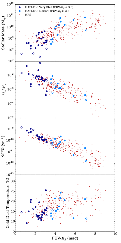
Figure 14: Scaling relations with FUV-$K_{S}$ colour for HAPLESS and the HRS. From top-to-bottom – 1^st: Stellar mass against FUV-$K_{S}$ colour. 2^nd: $M_{d}/M_{\star}$ (ie, specific dust mass) against FUV-$K_{S}$ colour, showing the strong relationship between colour and dust-richness. 3^rd: SSFR against FUV-$K_{S}$ colour; the two are tightly related, with our FUV-$K_{S}$ < 3.5 colour criterion corresponding to a SSFR $\sim 1.1\times 10^{-10}\,{\rm yr^{-1}}$. 4^th: Cold dust temperature against FUV-$K_{S}$ colour; HAPLESS shows a preponderance of cold blue galaxies, which only make up a small fraction of the HRS.

Figure 15: Scaling relations with $L_{\it FUV}/L_{\it TIR}$ for the HAPLESS and HRS. Upper: Cold dust temperature against $L_{\it FUV}/L_{\it TIR}$. Centre: $M_{d}/M_{\star}$ against $L_{\it FUV}/L_{\it TIR}$; counter-intuitively, the more dust-rich a galaxy, the larger the proportion of FUV photons that go unabsorbed. Lower: FUV-$K_{S}$ colour against $L_{\it FUV}/L_{\it TIR}$; correlation is very tight for bluer galaxies, but far weaker for redder galaxies.

We compare the relative rates of star formation activity between the samples using specific star formation rate (SFR/$M_{\star}$), with distributions shown in Figure 12. The HAPLESS galaxies tend towards higher SSFRs, with a median of $1.3\times 10^{-10}\,{\rm yr}^{-1}$. Only 15 per cent (34 per cent) of the HRS (Planck C13N13) galaxies exhibit SSFRs greater than this. The difference in SSFR distrbutions is statistically significant (Table 6), again highlighting that the HRS stellar mass selection appears to under-sample the regions of the parameter space where the blindly-selected galaxies are found.

Figure 13 (top) shows the cold dust temperature distributions of the three samples. The HRS and Planck C13N13 distributions are similar, with medians of 18.5 and 17.7 K respectively (Table 6). The HAPLESS distribution, however, is strikingly different, with a broad peak in the 10–17 K range and a median temperature of 14.6 K; 71 per cent (30) of the HAPLESS galaxies have dust temperatures colder than both the HRS and Planck C13N13 medians.

The relationship between cold dust temperature and galaxy morphology for the three samples is shown in the 2^nd panel of Figure 13. A strong correlation is present; the dust in later galaxy types tends to be much colder than in low metallicity dwarf galaxies (Rémy-Ruyer et al., 2013) and in earlier types (Skibba et al., 2011; Smith et al., 2012c). The HAPLESS galaxies are heavily skewed towards the late type and very cold end of the distribution. The 3^rd panel of Figure 13 compares stellar mass with cold dust temperature. Only a weak correlation is seen (the Spearman rank coefficients are 0.23, 0.39 and 0.23 for the HAPLESS, HRS and Planck C13N13 samples respectively; only the latter two samples are statistically significant). We note that Bourne et al. (2012) find a correlation between dust temperature and stellar mass for blue cloud galaxies using a stacking analysis on the H-ATLAS data; this trend is plotted as the dashed line.

The last panel of Figure 13 shows a strong inverse correlation between cold dust temperature and $M_{d}/M_{\star}$, this is particularly tight for galaxies with cold dust temperatures below $\sim$ 15 K. We will explore physical connections between stellar heating sources and dust temperature next but first we consider whether this trend could be related to selection biases. As it is always easier to detect a warm dust source at a given mass than a colder one, the lack of galaxies in the upper right of this plot cannot be a selection bias. If galaxies existed in this part of parameter space (high dust content and warm) we would see them. We interpret this as a ‘heating limit’ – there is simply not enough stellar radiation available to heat the dust present above the upper temperature envelope. On the other hand, the lack of cold galaxies with low $M_{d}/M_{\star}$ (lower left) may well be due to the detection bias against low dust mass objects with cold temperatures discussed in Section 5.4. Warmer galaxies can still be above the flux limit with smaller quantities of dust, and there is indeed more scatter to lower $M_{d}/M_{\star}$ values at higher dust temperatures. The curves in Figure 13 show our observing limits (for inclusion in the luminosity-limited subset of our sample) of $M_{d}/M_{\star}$ as a function of temperature for different values of $M_{\star}$. This explains the lack of sources in the lower left region of this plot and the apparent ‘tightening’ of the relationship at cold temperatures.

Comparing our parameters with FUV-$K_{S}$ colour instead of dust temperature in Figure 14 shows very tight scaling relations of colour against stellar mass, $M_{d}/M_{\star}$, and SSFR. The 2^nd panel of Figure 14 demonstrates that bluer galaxies are consistently more dust-rich. We see that across the 3.5 orders of magnitude of $M_{d}/M_{\star}$ sampled by HAPLESS and the HRS, no galaxies are so dusty that extinction takes over and FUV-$K_{S}$ colours become redder. This is in stark contrast to the Dust-Obscured Galaxies (DOGs) and SMGs observed at higher redshifts, where dust-richness gives rise to severe extinction, resulting in red UV-NIR colours (Dey et al., 2008; Calanog et al., 2013; Rowlands et al., 2014a).

Despite blue FUV-$K_{S}$ colours indicating plentiful ongoing star formation (Figure 14, 3^rd panel) there is no correlation between ‘blueness’ and dust temperature (Figure 14, 4^th panel). However, many of the curious blue galaxies are found to have very cold dust temperatures. A possible explanation for this is that a large fraction of their UV luminosity escapes unabsorbed by dust. In Figure 15 we examine $L_{\it FUV}/L_{\it TIR}$ in relation to dust temperature, $M_{d}/M_{\star}$, and FUV-$K_{S}$ colour. $L_{\it FUV}/L_{\it TIR}$ indicates the number UV photons escaping a galaxy (unabsorbed), relative to the amount of energy which is absorbed by dust and thermally re-emitted in the IR. In the case where most dust emission is powered by absorption of UV photons rather than optical photons, this is equivalent to a measure of the UV transparency. Overall, both the HAPLESS and HRS samples show that the cold dust temperature is anti-correlated with $L_{\it FUV}/L_{\it TIR}$, suggesting that the higher the factor of UV radiation that is absorbed, the higher the temperature of the cold dust. The very bluest HAPLESS galaxies have the highest values of $L_{\it FUV}/L_{\it TIR}$, and display a range of cold dust temperatures. The central panel of Figure 15 shows that, counter-intuitively, the more dust-rich a galaxy is (as defined by $M_{d}/M_{\star}$), the smaller the fraction of the UV luminosity that suffers dust absorption. The combination of dust-richness and low attenuation leads to the very cold dust temperatures in the bluest galaxies. This could be due to some physical difference in the grain population, leading to more efficient emission and/or less efficient absorption in the UV; or due to a difference in the dust-star geometry in the bluest sources. This is beyond the scope of this work but be will explored further using the James et al. (2002) method and radiative transfer modelling respectively (Dunne et al., in prep., De Vis et al., in prep.).

The lower panel of Figure 15 demonstrates a tight correlation between $L_{\it FUV}/L_{\it TIR}$ and FUV-$K_{S}$ colour – except for galaxies on the red sequence (FUV-$K_{S}$ $\gtrsim$ 6). In these systems there is a range of $L_{\it FUV}/L_{\it TIR}$ at the same colour. Recalling that $L_{\it FUV}/L_{\it TIR}$ is really only an attenuation measure if most IR luminosity is powered by UV photons (as opposed to optical ones), this wide range of values for $L_{\it FUV}/L_{\it TIR}$ on the red sequence may indicate that the dust heating in this population is not dominated by UV radiation. Dust in early type galaxies is often acquired during interactions (Gomez et al., 2010; Smith et al., 2012c; Rowlands et al., 2012) which may produce a range of dust geometries and therefore a wide range of values for $L_{\it FUV}/L_{\it TIR}$.

In summary, the bluest FUV-$K_{S}$ sources exhibit the highest SSFRs, the highest specific dust masses, the lowest UV attenuation and often display very cold temperatures.

5.5.1   What is Heating the Cold Dust Component?

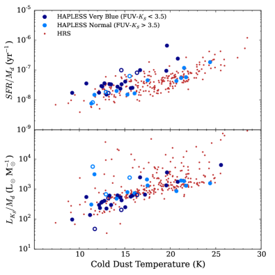
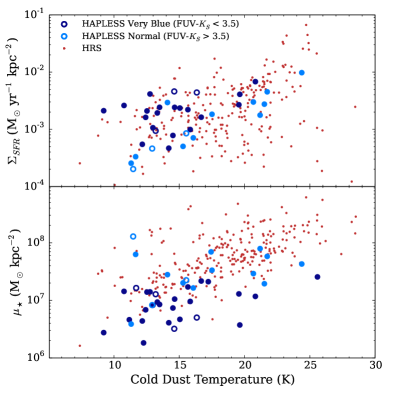
Figure 16: The influence of star formation and the older stellar population upon the temperature of the cold dust in the HAPLESS and HRS galaxies. Upper left: ${\it SFR}/M_{d}$. Lower left: $L_{K_{S}}/M_{d}$. Upper right: SFR surface density, $\Sigma_{\it SFR}$. Lower right: Stellar mass surface density, $\mu_{\star}$.

Dust heating in galaxies can occur in a variety of ways (see Kennicutt & Evans, 2012; Dunne, 2013). Warm dust is thought to be associated with star-forming dense molecular clouds, with newly formed stars heating the dust to temperatures > 30 K (Kennicutt, 1998; Kennicutt et al., 2009; Bendo et al., 2010). Cold dust is usually associated with the diffuse ISM (Rowan-Robinson & Crawford, 1989; Boulanger et al., 1996; Lagache et al., 1998; Tuffs & Popescu, 2005; Boquien et al., 2011; Bendo et al., 2012). Most dust resides in this diffuse environment (Dunne & Eales, 2001; Draine et al., 2007) where it is heated by the general InterStellar Radiation Field (ISRF), and is often known as a ‘cirrus’ component (Rowan-Robinson & Crawford, 1989). The ISRF may be largely composed of photons in the optical produced by the old stellar population; in this case, the cold dust luminosity would be powered by the old stellar population and not young newly formed stars (Tuffs & Popescu, 2005; Boquien et al., 2011; Bendo et al., 2012). However, it is also possible that high energy UV photons from low optical depth star forming regions could ‘leak out’ and therefore contribute to heating the diffuse dust component (Law et al., 2011; Popescu et al., 2011; Clemens et al., 2013; Hughes et al., 2014). The dust heating will also depend on the distribution of dust and stars within a galaxy and the optical properties of the dust (see Foyle et al., 2013). Bendo et al. (2014) recently used a large number of sources from the Very Nearby Galaxy Survey, HRS, and KINGFISH to show that the relative contributions of young and evolved stars to dust heating varies greatly among nearby spiral galaxies. In this section, we wish to investigate the relative importance of both the young and the old stellar population in heating the bulk dust mass (ie, the cold component).

Our choice of ‘heating’ parameter is influenced by the study of Foyle et al. (2013) who proposed that the amount of star formation (or alternatively old stellar luminosity) per unit dust mass should determine the temperature of the bulk dust component, not simply the amount of star formation and/or old stars (ie, SFR/stellar mass) or even their surface density. If there is more dust to be heated by a particular radiation field then its average temperature will be lower. To explore this, Figure 16 (left column) compares SFR/$M_{d}$ (a proxy for energy in star formation per unit dust mass) and $L_{K_{S}}/M_{d}$ (a proxy for the energy in old stellar photons per unit dust mass) with the cold dust temperature.

In the upper panel we see that higher values of ${\it SFR}/M_{d}$ correlate with higher values of $T_{c}$ with Spearman $r$ coefficient of 0.74 for the combined surveys ($r=0.71$ for HAPLESS, $r=0.75$ for HRS). This was also seen in Planck C13N13. In the lower panel, a positive correlation is seen between $L_{K_{S}}/M_{d}$ and $T_{c}$ (Spearman coefficient $r=0.69$ for the combined surveys – $r=0.64$ and $r=0.67$ for the HAPLESS and HRS respectively) with most sources clustered together with a well-defined maximum described by $T_{\it max}\sim(L_{K_{S}}/M_{d})^{0.25}$. The galaxies which scatter well above this tight cluster of sources are early-types (E and S0). These relationships suggest that both star formation and the old stellar population are important contributors to the heating of the diffuse dust component in these samples, (first noted for the HRS by Boselli et al. 2012). On average, we also see that for a given value of $T_{c}$, the ${\it SFR}/M_{d}$ is higher in the HAPLESS sources compared to the HRS, whereas this is not the case when comparing $L_{K_{S}}/M_{d}$.

Kirkpatrick et al. (2014) make the same comparison in a study of a sample of resolved star forming spirals with average $M_{\star}=8.2\times 10^{9}\,\rm M_{\odot}$ from the KINGFISH survey. They use 500 µm luminosity as a proxy for dust mass, 3.6 µm luminosity to trace the the older stellar population, and H$\alpha+24\,\mu$m emission to trace SFR in a study of star-forming spirals. They find a similar relationship between SFR per unit dust mass and temperature; however in contrast to this work they find no significant correlation between the old stellar luminosity per dust mass and temperature. A key difference in our approach compared to theirs is that they consider resolved regions within their galaxies and so photons are required to be absorbed within the same pixel they were emitted in order to produce a correlation. It is not clear whether the Kirkpatrick et al. (2014) sample would produce the same trends as we see if only the global integrated values were considered.

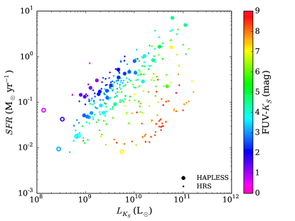
Figure 17: The relationship between $L_{K_{S}}$ and ${\it SFR}$, colour-coded by FUV-$K_{S}$ colour (indicating morphology), for the HAPLESS and the HRS galaxies. Hollow circles show galaxies beneath the luminosity limit of the sample.

A sufficiently tight, linear correlation between $L_{K_{S}}$ and SFR could make it appear that cold dust temperature is correlated with the heating parameter ${\it SFR}/M_{d}$, even if $L_{K_{S}}$ alone was driving the cold dust temperature, with no contribution from star formation (and vice-a-versa). To test for this, we plot $L_{K_{S}}$ against SFR in Figure 17. A tight, linear relation in this plot could give rise to spurious correlations with temperature in Figure 16. However, the scatter in this plot is in fact very large – almost 2 orders of magnitude in SFR are possible for a given value of $L_{K_{S}}$, with distinct sequences of ETGs and LTGs (as indicated by their FUV-$K_{S}$ colour) visible. Given how weak the correlation in this plot is (Spearman rank correlation coefficient of 0.28 with both samples taken together), it does not seem possible that it could be artificially driving the tight relations in the left-hand panels of Figure 16 (which have Spearman rank correlation coefficients of 0.74 and 0.69 respectively). This was corroborated by using Monte-Carlo simulations of the $L_{K_{S}}$ against SFR relation to generate ‘spurious’ versions of the heating relations in the left half of Figure 16; the ‘spurious’ simulated plots were never able to replicate the degree to which the actual heating relations are tighter than the $L_{K_{S}}$ vs SFR relation.

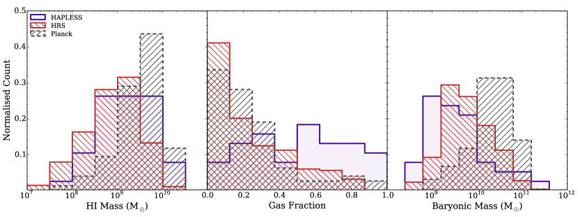
Figure 18: The atomic gas properties of the HAPLESS, HRS, and Planck C13N13 galaxies. Left: The Hi mass distribution. Centre: The gas fraction (Equation 6). The HAPLESS sources have higher gas fractions than seen in other FIR surveys of local galaxies. Right: The baryonic mass distribution. Whilst the stellar mass and Hi mass distributions of HAPLESS and the HRS are very different, their baryonic mass distributions are rather more similar.

We also show the relations between the surface densities of star formation ($\Sigma_{\it SFR}$) and stellar mass ($\mu_{\star}$) against $T_{c}$ in Figure 16 (right column). The surface density of SFR and the old stellar population should be a first approximation to the average ISRF contributed by both populations (the energy per unit area), although this assumption is complicated in the case of the SFR surface density, as some fraction of the UV radiation will be absorbed locally by dust in the birth clouds and contribute to heating the warm dust component rather than the cold.

Both the HAPLESS and HRS (see also Boselli et al. 2012) show a clear correlation between $\mu_{\star}$ and $T_{c}$ ($r=0.44$ and $r=0.63$ respectively, with $r=0.65$ when the two samples are combined); the stellar mass surface density is also higher for HRS galaxies at a given dust temperature. Further evidence for heating by the old stellar population comes from the sample of H-ATLAS galaxies in Bourne et al. (2013) (of which 12 overlap with our sources) using independent measurements of correlations with dense and diffuse gas components.

Additionally, the HAPLESS galaxies show a weak, but significant correlation between star formation surface density and cold dust temperature ($r=0.32$) while, in contrast, the HRS shows no significant correlation ($r=0.04$). More specifically, the HAPLESS sample shows a range of $\Sigma_{\it SFR}$ at the coldest dust temperatures, but requires a higher $\Sigma_{\it SFR}$ to reach higher temperatures; the HRS sample instead shows a range of $\Sigma_{\it SFR}$ at all temperatures.

This suggests that while both the young and old stellar radiation fields play a role in heating the dust in both samples, the HRS dust heating is more strongly influenced by the old stellar population while HAPLESS sources are on average more strongly heated by the young stellar population. As the average stellar mass and SSFR of HAPLESS are lower and higher respectively than HRS, finding an ISRF dominated by young stars is not surprising in the HAPLESS systems.

5.6   Gas Properties

Here we compare the gas properties of the three samples. Figure 18 shows the Hi mass distribution of the three samples; 90 per cent (38) of the HAPLESS galaxies, 81 per cent (263) of the HRS, and 94 per cent (220) of the Planck C13N13 galaxies have Hi data available. Interestingly, the median HAPLESS Hi mass of $1.4\times 10^{9}\,{\rm M}_{\odot}$ is greater than the HRS median – despite the median HAPLESS stellar mass being 4 times lower than that of the HRS. Once again, the bias of the Planck C13N13 sample towards more massive objects is manifest (Table 6).

The Hi gas fractions (Equation 6) of the HAPLESS galaxies have a median value of 0.52 (Table 6), and show a relatively flat distribution from 0.03 to 0.96, spanning a much wider range than those in HRS or Planck C13N13. Of the HAPLESS galaxies with Hi detections, 58 per cent (18) have baryonic masses which are in fact dominated by their atomic gas component. This is without any consideration of molecular gas, the inclusion of which would only serve to drive up the gas fractions still further. In contrast, the HRS and Planck C13N13 distributions are strongly skewed towards lower gas fractions, with medians of 0.18 and 0.17 respectively. A K-S test suggests that HAPLESS galaxies are drawn from a different underlying population in terms of gas fraction (Table 6).

The right hand panel of Figure 18 shows the baryonic masses of the three samples, where $M_{B}=M_{\it HI}+M_{\star}$. This measure of galaxy mass may be more appropriate for comparing samples where stars make up only a small fraction of the total baryonic mass of some of the galaxies. Whilst HAPLESS and the HRS have very different distributions of stellar mass and Hi mass (Figures 9 and 18), the differences are far less pronounced once we consider baryonic mass (see Table 6). ThePlanck C13N13 sample is again limited by its high 550 µm flux limit, primarily sampling galaxies with high baryonic masses. In the local Universe – where the largest halos have already completed more of their star formation – this tends to populate the Planck C13N13 sample with a relatively high fraction of passive, high stellar mass and low gas fraction galaxies.

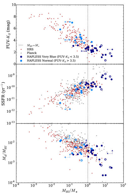
Figure 19: Trends with $M_{\it HI}/M_{\star}$ (ie, gas richness) for the HAPLESS, HRS and Planck C13N13 samples. Upper: FUV-$K_{S}$ versus $M_{\it HI}/M_{\star}$. Bluer colours are strongly associated with higher gas-to-stellar mass fractions; The (FUV-$K_{S}$ < 3.5) colour-criterion we use to define the curious very blue galaxies transpires to correspond to $M_{\it HI}\approx M_{\star}$ (vertical dotted line). Centre: $M_{\it HI}/M_{\star}$ against SSFR. Lower: $M_{d}/M_{\it HI}$ against $M_{\it HI}/M_{\star}$. Hollow circles indicate galaxies that are beneath the luminosity-limit of the sample. HIPASS 3 $\sigma$ upper limits (Equation 5) are shown (dotted in the case of galaxies not in our 250 µm luminosity-limit sub-sample.)

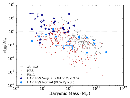
Figure 20: $M_{\it HI}/M_{\star}$ against the baryonic mass of the HAPLESS, HRS and Planck C13N13 samples. The dotted line indicates $M_{\it HI}/M_{\star}=1$. Symbols as in Figure 19.

In Figure 19, we consider the properties of the galaxies in relation to their atomic gas richness; ie, $M_{\it HI}/M_{\star}$. The top panel shows that bluer FUV-$K_{S}$ colour is strongly correlated with higher levels of gas richness; we also note that the edges of this distribution appear to be quite sharp; for a given FUV-$K_{S}$ colour, only a small range of $M_{\it HI}/M_{\star}$ seems permissible. This is also seen in the correlation between FUV-$K_{S}$ colour and SSFR (Figure 14), and together with the middle panel, shows that SSFR is strongly related to gas fraction in the local Universe. This relation will be explored further in a companion paper (De Vis et al., in prep.) The curious blue HAPLESS galaxies (FUV-$K_{S}$ < 3.5) are the most gas-rich of all; 80 per cent of those with Hi detections contain a greater mass of Hi than of stars, and their median gas fraction is 0.66. Conversely, all but one of the HAPLESS sources with $M_{\it HI}/M_{\star}>1$ are in the curious blue category. It transpires that the (FUV-$K_{S}$ < 3.5) colour criterion we adopted to identify the curious very blue galaxies corresponds to the divide between galaxies whose baryonic mass is gas-dominated, and those which are star-dominated.

The dust-to-gas ratio of the samples ($M_{d}/M_{\it HI}$) are compared in the lower panel of Figure 19. Until now we have described the HAPLESS galaxies, especially the curious blue subset, as being very dust-rich compared to other FIR surveys, in light of their high values of $M_{d}/M_{\star}$. But the HAPLESS galaxies are in fact dust-poor relative to their gas mass. The median value (see Table 6) of $M_{d}/M_{\it HI}$ for the HRS and Planck C13N13 galaxies are $6.2\times 10^{-3}$ and $1.2\times 10^{-2}$ (ie, gas-to-dust ratios of $\approx\,160$ and $\approx\,90$), whilst the median for the HAPLESS galaxies is $3.9\times 10^{-3}$ (gas-to-dust $\approx\,260$). Furthermore, the median $M_{d}/M_{\it HI}$ of the curious blue subset is only $2.7\times 10^{-3}$ – a median gas-to-dust ratio of ${\it\approx\,370}$. In comparing dust-to-gas ratios of high and low gas fraction samples in this way, we do need to worry about our lack of molecular gas information. The Planck C13N13 and HRS may have higher $H_{2}$/Hi ratios than the higher gas fraction HAPLESS sources (Saintonge et al., 2011) and so the difference in dust-to-gas ratio may be less when this is taken into account. The dust properties in relation to gas-richness will be explored further in De Vis et al. (in prep).

Figure 20 compares baryonic mass to $M_{\it HI}/M_{\star}$ for the HAPLESS, HRS, and Planck C13N13 galaxies. Across all three samples, we see a trend where galaxies with large baryonic masses tend to have depleted more of their gas than smaller objects, though the Planck C13N13 galaxies tend to have higher gas-to-stellar mass ratios for a given baryonic mass. As the HRS is essentially a stellar-mass-selected sample, it is biased towards objects that have already converted a large fraction of their gas into stars. The high flux limit of the Planck C13N13 sample means that it is biased towards more massive galaxies; but being selected by dust brightness, it nonetheless tends to select the more ISM-rich examples of these massive systems. Our blind submm HAPLESS sample favours ISM-rich objects and consistently features the most gas-rich galaxies of a given baryonic mass.

6   The Evolution of Gas and Dust

Here, we will attempt to explain the dust masses and high gas fractions of the HAPLESS sources using a chemical and dust evolution model to follow the build up of heavy elements and dust over time as gas is converted into stars. We assume a closed box model as the optimistic case for the build up of dust (that is, we do not consider inflows and outflows of gas) and instead simply follow the gas (and gas fraction $f_{g}$) as it is converted into stars using a star formation rate $\psi(t)$ and an IMF $\phi(m)$ (using the Chabrier, 2003 IMF consistent with Sections 4.2 and 4.4). More details of the model can be found in Appendix B; see also Morgan & Edmunds (2003) and Rowlands et al. (2014b).

We assume two possible scenarios for dust formation by stars (see Rowlands et al., 2014b for a more in depth discussion): firstly, where dust is only contributed via the stellar winds of evolved Low-to-Intermediate Mass Stars (LIMS); and secondly, where dust is contributed via both LIMS and SuperNovae (SNe). Whether the majority of dust in galaxies is contributed by LIMS or SNe is a long-standing question (see the review in Gomez, 2013), though recent results (Gall et al., 2014) suggest not only do SNe form significant quantities of dust, but that also these grains are big enough (>1 µm) to survive their journey through the harsh reverse shock. We use the dust yields from LIMS consistent with FIR observations (Ladjal et al., 2010) and theoretical models (Ventura et al., 2012). For supernova dust yields, we use those of Todini & Ferrara (2001), which are consistent with the upper range of dust masses observed in historical SN remnants including the Crab Nebula (Gomez et al., 2012b; Owen & Barlow, submitted.), Cassiopeia A (Dunne et al., 2003, 2009; Rho et al., 2009; Barlow et al., 2010), and SN1987A (Matsuura et al., 2011; Indebetouw et al., 2014). Type-Ia SNe are assumed to be negligible contributors to the dust budget (Morgan et al., 2003; Gomez et al., 2009, 2012a). Note that we have no dust destruction in our model as we want to follow the maximum build up of dust mass at a given time (see Rowlands et al., 2014b).

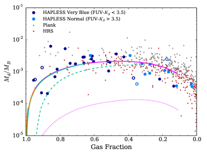
Figure 21: $M_{d}/M_{B}$ against gas fraction for the three samples. Note that the x-axis of this plot goes from a gas fraction of 1 to 0. The curves show the results from the chemical evolution model for different SFHs (Appendix 25, Table 8) including SFR A - consistent with the Milky Way (purple, Yin et al., 2009); SFR B - exponentially declining SFR with initial value of $0.06\,\rm M_{\odot}\,yr^{-1}$ and a burst (orange); SFH C - an exponentially declining rate, but with higher initial SFR of $2.4\,\rm M_{\odot}\,yr^{-1}$ (tourquoise); and finally SFR D - a scaled version of SFR C ($\times\,20$, tourquoise dashed). The dotted purple line is SFH A (MW) with dust from LIMS only.

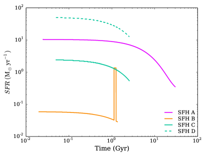
Figure 25: The star formation histories used to model the HAPLESS galaxies. SFH A follows the evolution of the MW (pink, uppermost solid track, Yin et al. 2009) with initial gas mass $M_{g}(0)=4\times 10^{10}\,\rm M_{\odot}$ and initial SFR $\psi(0)=\rm 10\,M_{\odot}\,yr^{-1}$. SFH B (orange, lowermost solid track) has initial gas mass $M_{g}(0)\sim 3\times 10^{9}\,\rm M_{\odot}$ and initial SFR $\rm 0.058\,M_{\odot}\,yr^{-1}$ with a burst at 1 Gyr superimposed on top of the exponentially declining rate. SFH C (orange, middle solid track) has $M_{g}(0)=5.5\times 10^{9}\,\rm M_{\odot}$ and initial SFR $\rm 2.4\,M_{\odot}\,yr^{-1}$ and exponentially declines until reaching a gas fraction of $f_{g}\sim 0.6$ at 2.5 Gyr. SFR D (turquoise, dashed track) is a scaled version of SFR C ($\times 20$).

We use four fiducial Star Formation Histories (SFHs), shown in Figure 25 and in Table 8, to model the HAPLESS galaxies. These SFHs are (i) SFH A - consistent with the Milky Way (Yin et al., 2009); (ii) SFH B - an exponentially declining SFR with initial value of $\psi(t,0)=0.06\,\rm M_{\odot}\,yr^{-1}$ and a short burst at $\sim 1$ Gyr; (iii) SFH C - a faster exponentially declining SFR than B, with initial SFR of $2.4\,\rm M_{\odot}\,yr^{-1}$; (iv) SFH D - a scaled-up version of SFR C (multiplied by a factor of 20) to illustrate the evolution of a galaxy which is consuming its gas more rapidly. Using these fiducial SFHs, we follow the evolution of the dust mass relative to the baryonic mass as the gas fraction falls. The initial gas mass is set to $M_{g}(0)=4\times 10^{10}\,\rm M_{\odot}$ for the Milky Way, and for the other models we use the observed gas masses and fractions (Table 4) to derive the initial gas masses (these range from $M_{g}(0)=3-5.5\times 10^{9}\,{\rm M_{\odot}}$).

The model results are shown in Figure 21. First, we compare the dust evolution with dust only from LIMS (dotted line). Second, including dust from LIMS and SNe in combination (solid and dashed lines). None of the models for the former scenario (ie, without SN dust) reach the high levels of $M_{d}/M_{B}$ observed in the HAPLESS, HRS and Planck C13N13 samples; this is in line with results from other studies, including Morgan & Edmunds (2003), Matsuura et al. (2009), Dunne et al. (2011), Gall et al. (2011), and Rowlands et al. (2014b). With dust from both SNe and LIMS, SFH models A–C all sit on the same evolutionary track in Figure 21, due to the models with lower star formation rates (SFHs B & C) than the MW (SFH A) also having lower initial gas masses; ie the models lie on the same constant $SFR/M_{\it HI}$ tracks. These are in good agreement with the HAPLESS galaxies (at high gas fractions) and the HRS galaxies at lower gas fractions. The Planck C13N13 galaxies (clustered towards lower gas fractions) have somewhat elevated $M_{d}/M_{B}$ compared to the models presented here. When we multiply SFH C by a factor of 20 (SFH D) but keep the initial gas mass the same as SFH C, the evolutionary path is offset, due to the available gas reservoir being consumed faster and dust mass reduced due to astration.

Table 8: The fiducial star formation histories (A–D) and initial gas masses used in this work to model the HAPLESS galaxies. SFH A is from Yin et al., 2009. Also given is the time ($t_{\rm end}$) where the SFH is truncated to match the present observed SFRs and gas fractions of the HAPLESS sample (Section 4).

SFH	$g(0)$	$\psi(0)$	Burst?	$t_{\rm end}$	$\psi(t_{\rm end})$	$f_{g}(t_{\rm end})$
	($\rm M_{\odot}$)	($\rm M_{\odot}\,yr^{-1}$)	(Y/N)	(Gyr)	($\rm M_{\odot}\,yr^{-1}$)
A (MW)	$4.0\times 10^{10}$	10	N	20	0.7	0.11
B	$3.0\times 10^{9}$	0.06	Y	1.35	0.029	0.95
C	$5.5\times 10^{9}$	2.5	N	2.8	0.5	0.64
D	$5.5\times 10^{9}$	49	N	0.1	48	0.31

The evolutionary path suggested in Figure 21 indicates that a galaxy’s dust mass will peak when its gas fraction falls to $\sim$ 0.5, as predicted in Eales & Edmunds (1996). Therefore this is the stage of a galaxy’s development when it is most likely to meet the inclusion threshold of a dust-selected sample such as HAPLESS – the median gas fraction of which is indeed 0.5. The stellar-mass selection of the HRS means that it is biased towards galaxies where most of the gas has already been converted into stars, hence it severely under-samples the gas-rich portion of this evolutionary path. Similarly, the tendency of the Planck C13N13 sample to mainly select more massive galaxies means that it too is biased towards systems with low gas fractions.

7   Conclusions

We have presented a dust-selected sample of nearby galaxies drawn from the blind H-ATLAS submm survey and introduced a pipeline used to derive photometry, dust masses and other properties for the sample. We have also studied correlations between the dust and other properties of the galaxies in our sample, and the HRS and Planck samples. We find the following results:

• A typical source seen by Herschel in this blind survey has a cold dust temperature of 14.6 K and dust mass of $5.6\times 10^{6}\,{\rm M}_{\odot}$.

• HAPLESS galaxies have median $M_{d}/M_{\star}$ greater by a factor of $\sim$ 3.7 than the galaxies observed as part of the Herschel Reference Survey, and a factor of 1.8 than galaxies in the Planck Early Release Compact Source Catalogue. The median properties of this sample include: $\langle M_{\star}\rangle=9.8\times 10^{8}\,\rm M_{\odot}$, $\langle{\rm SFR}\rangle=0.2\,\rm M_{\odot}\,yr^{-1}$, $\langle{\rm SSFR}\rangle=1.3\times 10^{-10}\,\rm\,yr^{-1}$ and are amongst the most actively star forming galaxies seen in local FIR and submm surveys.

• This sample contains a high proportion of very blue galaxies (defined as FUV-$K_{S}$ $<$ 3.5). These are generally irregular and/or highly flocculent; such galaxies tend to be UV-bright, NIR-faint, dust rich, and low stellar mass, with high specific star formation rates. The median dust-to-stellar mass ratio of the very blue subset is $\sim$ 3–5 times larger than the Planck and HRS samples. Whilst accounting for only 6 per cent of the stellar mass in our sample, the bluest galaxies in our sample contain over 35 per cent of the dust mass.

• The dust mass volume density of our sample is $(3.7\pm 0.7)\times 10^{5}{\rm\,M_{\odot}\,Mpc^{-3}}$, which is higher than some other estimates, but consistent with the value found by Planck. Much of this difference seems to arise from the low dust temperatures of the galaxies in our sample, as the 250 µm luminosity function of our sample is in good agreement with surveys of larger volumes. Note however that our volume suffers from a high cosmic variance of $\sim$ 166 per cent.

• The HAPLESS galaxies are extraordinarily gas rich, particularly the very blue sources. Of the 38 HAPLESS galaxies detected in Hi, 21 (55 per cent) have atomic gas masses greater than or equivalent to their stellar mass. Their median gas fraction is 0.52, and 26 per cent have gas fractions $>\,0.8$. The median gas to dust ratios of these sources (> 260) is 1.6–3.0 times greater than for the other local samples of dusty galaxies.

• The coldest dust seen in the local universe is consistently associated with galaxies that have lots of star formation relative to their older stellar population. Despite dust being so plentiful in these objects, UV photons apparently go unabsorbed – giving rise to their very blue FUV-$K_{S}$ colours, and colder dust temperatures. Comparing the star formation and stellar mass surface densities also shows that dust heating in galaxies selected by HRS is more strongly influenced by the old stellar population whereas galaxies selected in HAPLESS are more strongly heated by the young stellar population.

• A chemical and dust evolution model confirms these galaxies are simply in an earlier stage of converting their gas into stars. The bluest galaxies appear to be the most immature; they should therefore provide valuable insights into the chemical evolution of young galaxies.

A blind dust-selected sample in the local universe reveals very blue, dusty, and gas-rich galaxies. Despite accounting for roughly half of all dusty galaxies, they have been severely under-represented in other FIR and submm surveys. We suggest the properties of these blue galaxies are in line with their ‘immaturity’, and therefore may provide useful analogues to very young, high-$z$ galaxies, though we note that the interstellar medium in the HAPLESS sources is likely to be different. Resolved atomic and molecular gas maps of the bluest sources in this sample, combined with radiative transfer modelling, 850 µm observations, and integrated optical spectra, should be able to address this and test whether these blue-but-dusty galaxies have different grain properties or whether the dust is distributed in a ‘leaky’ geometry (De Vis. et al., in prep., Dunne et al., in prep., Smith et al., in prep.).

8   Acknowledgements

CJRC acknowledges support from the Science and Technology Facilities Council (STFC) Doctoral Training Grant scheme and the European Research Council (ERC) FP7 project DustPedia (PI J Davies), and kindly thanks Marcel Clemens, Luca Cortese, Allison Kirkpatrick, Ivan Baldry, Lee Kelvin, and Michal Michalowski for helpful conversations. HLG and SAE acknowledge support from the STFC Consolidated Grant scheme. LD, SJM and RJI acknowledge support from the ERC in the form of the Advanced Investigator Program, COSMICISM. KR acknowledges support from the ERC Starting Grant SEDmorph (PI V Wild). The H-ATLAS is a project with Herschel, which is an ESA space observatory with science instruments provided by European-led Principal Investigator consortia and with important participation from NASA. The H-ATLAS website is http://www.h-atlas.org/. GAMA is a joint European-Australasian project based around a spectroscopic campaign using the Anglo-Australian Telescope. The GAMA input catalogue is based on data taken from the Sloan Digital Sky Survey and the UKIRT Infrared Deep Sky Survey. Complementary imaging of the GAMA regions is being obtained by a number of independent survey programs including GALEX MIS, VST KIDS, VISTA VIKING, WISE, Herschel-ATLAS, GMRT, and ASKAP, providing UV to radio coverage. GAMA is funded by the STFC (UK), the ARC (Australia), the AAO, and the participating institutions. The GAMA website is: http://www.gama-survey.org/. The authors gratefully acknowledge Martha Haynes, Riccardo Giovanelli, and the ALFALFA team for supplying the latest ALFALFA survey data.

This research has made use of Astropy, a community-developed core Python package for Astronomy (Astropy Collaboration et al., 2013). This research has made use of TOPCAT (Taylor, 2005), which was initially developed under the UK Starlink project, and has since been supported by PPARC, the VOTech project, the AstroGrid project, the AIDA project, the STFC, the GAVO project, the European Space Agency, and the GENIUS project. This research has made use of of APLpy, an open-source astronomical image plotting package for Python. This research has made use of NumPy (Walt et al., 2011), SciPy, and MatPlotLib (Hunter, 2007). This research has made use of the SIMBAD database (Wenger et al., 2000) and the VizieR catalogue access tool (Ochsenbein et al., 2000), both operated at CDS, Strasbourg, France. This research has made use of SAOImage DS9, developed by the Smithsonian Astrophysical Observatory with support from the Chandra X-ray Science Center (CXC), the High Energy Astrophysics Science Archive Center (HEASARC), and the JWST Mission office at the Space Telescope Science Institute (STSI). This research has made use of the NASA/IPAC Extragalactic Database (NED) and the NASA/IPAC Infrared Science Archive (IRSA), both operated by the Jet Propulsion Laboratory, California Institute of Technology, under contract with the National Aeronautics and Space Administration.

Appendix A Properties of the HAPLESS Galaxies

Multiwavelength imagery of the HAPLESS galaxies can be found in Figure A1. Our UV to FIR photometry of the HAPLESS galaxies, with uncertainties, is given in Table A1. Figure A2 shows the spectral energy distributions of the HAPLESS galaxies.

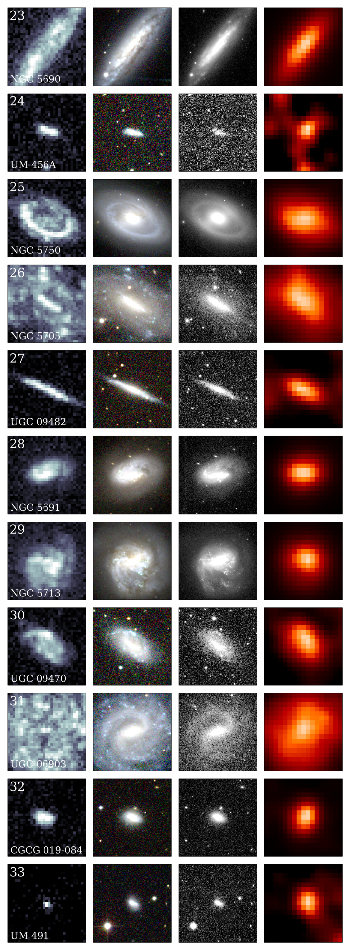
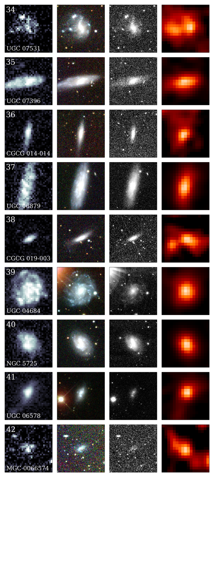
Figure 23: continued

Table 9: Photometry of the HAPLESS galaxies, where ’-’ indicates cases where no observations were available. The semi-major axis is denoted by $a$, the position angle by $\theta$, and the axial ratio (the semi-major axis divided by the semi-minor axis) by $a/b$. Herschel-SPIRE fluxes were measured using maps reduced for extended-source photometry, but have not been colour-corrected.

HAPLESS	Aperture dimensions			GALEX (mag)				SDSS (mag)								VIKING (mag)
	$a$ (arcsec)	$\theta$ (deg)	$a/b$	FUV	$\Delta$ FUV	NUV	$\Delta$ NUV	$u$	$\Delta\,u$	$g$	$\Delta\,g$	$r$	$\Delta\,r$	$i$	$\Delta\,i$	$Z$	$\Delta\,Z$
1	28.4	158.2	1.075	15.78	0.05	15.23	0.03	14.57	0.10	13.72	0.04	13.26	0.05	13.06	0.06	12.83	0.07
2	36.5	23.8	1.064	16.67	0.05	16.36	0.03	15.84	0.33	15.08	0.06	14.83	0.07	14.72	0.10	14.59	0.08
3	122.0	72.8	1.477	14.48	0.05	14.18	0.03	13.53	0.22	12.72	0.06	12.42	0.06	12.23	0.08	12.14	0.07
4	36.6	28.0	1.437	17.31	0.05	16.94	0.03	15.96	0.13	15.00	0.05	14.51	0.06	14.28	0.07	14.18	0.07
5	36.5	0.7	1.381	18.08	0.10	17.41	0.03	16.41	0.37	15.29	0.06	14.84	0.07	14.61	0.09	14.47	0.07
6	178.9	117.2	1.455	13.69	0.05	12.99	0.03	11.99	0.11	10.68	0.04	10.10	0.05	9.76	0.06	9.54	0.07
7	178.9	85.3	3.424	14.58	0.05	14.08	0.03	13.54	0.30	12.41	0.04	12.04	0.05	11.82	0.06	-	-
8	65.0	141.2	1.292	15.47	0.05	15.14	0.03	14.46	0.19	13.67	0.05	13.37	0.06	13.15	0.07	13.08	0.07
9	122.0	178.5	1.533	15.35	0.05	15.08	0.03	14.89	0.39	13.82	0.08	13.78	0.12	13.53	0.12	13.63	0.22
10	126.0	62.1	2.058	15.14	0.07	14.61	0.03	13.68	0.20	12.20	0.05	11.58	0.05	11.26	0.06	10.99	0.07
11	85.3	50.2	3.665	17.36	0.05	16.75	0.03	15.62	0.38	14.53	0.05	14.09	0.06	13.90	0.07	13.72	0.07
12	44.6	147.2	1.568	17.08	0.05	16.65	0.03	15.78	0.17	14.88	0.06	14.47	0.06	14.29	0.08	14.07	0.07
13	24.3	67.3	1.347	18.80	0.05	18.38	0.03	17.26	0.42	16.39	0.08	15.93	0.07	15.75	0.11	15.60	0.09
14	134.2	63.9	1.205	13.90	0.06	13.52	0.03	12.82	0.13	11.87	0.05	11.45	0.05	11.33	0.06	11.16	0.07
15	32.5	46.2	1.289	18.42	0.05	17.79	0.03	16.49	0.24	15.37	0.06	14.89	0.06	14.62	0.09	14.57	0.07
16	69.1	32.2	2.122	17.14	0.05	16.50	0.03	15.19	0.20	14.02	0.05	13.52	0.05	13.23	0.07	13.03	0.07
17	44.7	139.4	1.156	16.41	0.05	16.16	0.03	15.77	0.28	15.08	0.06	14.87	0.08	14.88	0.12	14.73	0.08
18	52.8	96.6	1.274	15.86	0.05	15.51	0.03	14.96	0.22	14.20	0.05	13.88	0.05	13.74	0.08	13.62	0.07
19	134.2	109.9	3.776	-	-	-	-	14.64	0.20	13.71	0.06	13.49	0.07	13.15	0.07	13.34	0.08
20	142.3	30.3	2.096	17.01	0.10	16.27	0.04	13.90	0.39	12.29	0.05	11.37	0.05	10.91	0.06	10.62	0.07
21	276.6	78.5	4.490	-	-	-	-	12.54	0.16	10.94	0.04	10.07	0.05	9.61	0.06	9.27	0.07
22	40.6	151.1	1.638	19.70	0.08	18.50	0.05	15.73	0.24	14.22	0.05	13.50	0.05	13.11	0.06	12.85	0.07
23	117.9	60.0	2.317	15.64	0.05	14.91	0.03	13.58	0.18	12.29	0.05	11.72	0.05	11.38	0.06	11.12	0.07
24	36.5	152.8	1.729	17.76	0.05	17.59	0.03	17.19	0.47	16.43	0.10	16.24	0.12	16.20	0.25	16.09	0.10
25	126.1	151.5	1.811	16.10	0.05	15.42	0.03	13.49	0.15	11.95	0.04	11.22	0.05	10.83	0.06	10.59	0.07
26	113.8	162.3	1.366	14.83	0.05	14.52	0.03	14.35	0.53	12.83	0.06	12.48	0.06	12.25	0.08	12.22	0.07
27	65.0	157.4	3.380	17.35	0.05	16.80	0.03	15.91	0.34	15.01	0.06	14.64	0.06	14.47	0.08	14.35	0.08
28	85.3	28.8	1.394	15.56	0.05	15.03	0.03	13.45	0.12	12.43	0.05	11.98	0.05	11.75	0.06	11.61	0.07
29	117.9	85.0	1.197	14.70	0.05	13.87	0.03	12.53	0.15	11.40	0.04	10.85	0.05	10.58	0.06	10.38	0.07
30	60.9	143.7	1.439	16.19	0.05	15.86	0.03	15.18	0.26	14.43	0.06	14.08	0.06	13.94	0.09	13.83	0.08
31	101.6	47.4	1.123	15.24	0.05	15.16	0.03	14.67	0.72	13.14	0.07	12.73	0.07	12.51	0.08	12.24	0.07
32	37.9	46.3	1.391	17.49	0.07	17.00	0.03	15.93	0.30	14.84	0.05	14.42	0.06	14.19	0.10	13.99	0.07
33	28.4	136.9	1.540	16.60	0.05	16.36	0.03	16.08	0.14	15.41	0.05	15.18	0.07	15.07	0.07	14.97	0.07
34	65.0	178.7	1.338	15.55	0.06	15.46	0.04	15.22	0.36	14.39	0.07	14.25	0.08	14.16	0.15	14.20	0.09
35	73.1	8.1	1.846	16.73	0.05	16.25	0.03	15.35	0.34	14.55	0.07	14.17	0.06	13.97	0.09	13.90	0.08
36	48.7	76.6	2.341	17.66	0.05	17.24	0.03	16.49	0.42	15.64	0.07	15.36	0.08	15.22	0.14	15.14	0.09
37	89.4	76.2	2.711	16.42	0.05	16.01	0.03	14.99	0.19	13.70	0.05	13.04	0.05	12.73	0.06	12.45	0.07
38	32.4	30.8	1.650	17.94	0.05	17.53	0.03	16.77	0.35	15.83	0.06	15.57	0.08	15.39	0.09	15.15	0.08
39	48.8	131.0	1.110	15.72	0.05	15.34	0.03	14.63	0.13	13.58	0.05	13.24	0.05	13.06	0.06	12.70	0.07
40	52.8	117.6	1.161	15.89	0.05	15.47	0.03	14.78	0.24	13.94	0.05	13.57	0.06	13.40	0.08	13.25	0.07
41	48.7	50.5	1.619	15.98	0.05	15.83	0.03	15.39	0.14	14.75	0.04	14.59	0.05	14.57	0.07	14.39	0.08
42	24.3	3.6	1.471	19.77	0.10	19.53	0.08	18.62	1.31	17.70	0.33	17.39	0.36	17.28	1.11	17.11	0.28

Table 10: continued

HAPLESS	VIKING (mag)								WISE (mJy)
	$Y$	$\Delta\,Y$	$J$	$\Delta\,J$	$H$	$\Delta\,H$	$K_{S}$	$\Delta\,K_{S}$	3.4 µm	$\Delta$ 3.4 µm	4.6 µm	$\Delta$ 4.6 µm	12 µm	$\Delta$ 12 µm	22 µm	$\Delta$ 22 µm
1	12.70	0.07	12.62	0.08	12.50	0.07	12.70	0.06	14.91	0.86	9.52	0.75	32.61	3.71	98.06	16.53
2	14.56	0.09	14.57	0.10	14.48	0.10	14.63	0.12	2.62	0.21	1.36	0.20	2.57	0.46	-	-
3	12.05	0.08	12.00	0.10	12.03	0.10	12.34	0.10	30.03	1.93	18.25	1.62	52.02	6.26	124.94	21.41
4	14.05	0.08	13.97	0.09	13.93	0.16	14.15	0.09	3.54	0.24	2.26	0.24	2.55	0.46	7.68	1.75
5	14.36	0.08	14.32	0.09	14.24	0.09	14.49	0.10	2.80	0.19	1.65	0.18	1.65	0.33	3.81	1.57
6	9.32	0.07	9.18	0.08	8.96	0.07	9.18	0.06	463.11	26.73	287.13	22.43	1287.59	146.06	1945.55	326.94
7	-	-	11.66	0.09	11.48	0.08	11.92	0.06	39.32	2.36	24.25	2.01	43.01	5.18	71.70	13.16
8	13.00	0.08	12.93	0.10	12.82	0.08	13.06	0.10	11.70	0.78	7.12	0.71	15.21	2.10	26.63	6.63
9	13.53	0.14	13.49	0.25	14.26	6.85	13.99	0.35	7.59	0.86	4.26	0.93	9.68	1.99	15.94	6.29
10	10.79	0.07	10.65	0.08	10.49	0.07	10.74	0.06	102.86	5.96	59.48	4.67	182.60	20.72	327.67	55.13
11	13.63	0.08	13.56	0.10	12.88	0.27	13.62	0.17	6.01	0.41	3.39	0.41	4.97	2.05	8.35	3.51
12	13.98	0.08	13.90	0.10	13.80	0.10	14.00	0.09	4.86	0.32	2.66	0.26	7.34	0.89	9.95	2.00
13	15.45	0.09	15.53	0.12	15.54	0.19	15.66	0.16	0.88	0.08	0.54	0.08	0.60	0.19	0.94	1.23
14	11.09	0.07	11.09	0.08	11.08	0.09	11.18	0.07	77.59	4.57	46.95	3.79	158.51	18.05	331.32	55.87
15	14.48	0.08	14.46	0.09	14.40	0.11	14.68	0.12	3.02	0.21	1.66	0.20	0.85	0.62	3.57	1.17
16	12.89	0.07	12.82	0.08	12.72	0.08	12.87	0.06	13.89	0.82	8.28	0.69	17.15	1.99	23.12	4.25
17	14.66	0.11	14.64	0.15	14.65	0.20	14.86	0.35	2.23	0.25	1.60	0.27	2.14	0.67	19.54	3.86
18	13.54	0.08	13.49	0.09	13.43	0.09	13.65	0.16	6.85	0.45	3.93	0.40	7.02	0.89	21.33	4.03
19	13.46	0.11	13.15	0.12	13.18	0.15	13.62	0.17	10.21	0.70	5.20	0.57	4.54	1.02	18.33	4.18
20	10.33	0.07	10.10	0.08	9.84	0.07	10.01	0.06	203.06	11.75	122.99	9.62	378.25	42.99	683.62	114.96
21	8.95	0.07	8.73	0.08	8.50	0.07	8.66	0.06	641.00	36.97	358.08	27.95	390.83	44.48	429.46	72.33
22	12.65	0.07	12.53	0.08	12.36	0.07	12.58	0.06	15.94	0.92	8.86	0.70	3.15	0.48	1.81	1.48
23	10.90	0.07	10.75	0.08	10.49	0.07	10.68	0.06	122.38	7.07	78.87	6.17	397.79	45.15	609.66	102.47
24	16.13	0.16	16.01	0.31	16.01	0.36	15.94	0.36	0.60	0.11	0.19	0.26	0.25	0.06	4.03	1.29
25	10.36	0.07	10.22	0.08	10.12	0.07	10.25	0.06	143.77	8.32	78.92	6.21	64.70	7.74	49.72	9.06
26	12.18	0.08	12.20	0.09	12.09	0.08	12.44	0.17	28.30	1.75	16.15	1.41	26.79	3.19	34.04	6.42
27	14.27	0.09	14.24	0.11	14.19	0.19	14.45	0.12	2.72	0.22	1.57	0.21	1.58	0.44	4.67	1.46
28	11.48	0.07	11.40	0.08	11.28	0.07	11.56	0.07	52.03	3.04	33.82	2.68	134.25	15.25	308.95	52.01
29	10.19	0.07	10.07	0.08	9.94	0.07	10.14	0.08	200.25	11.59	134.95	10.57	947.13	107.46	2427.67	408.04
30	13.79	0.11	13.80	0.11	13.81	0.26	13.95	0.13	5.53	0.40	2.95	0.40	2.56	0.53	13.02	2.79
31	12.17	0.08	12.11	0.10	12.05	0.09	12.29	0.13	25.93	1.71	15.75	1.45	31.86	5.48	28.27	7.75
32	13.86	0.08	13.82	0.09	13.71	0.08	13.89	0.09	5.42	0.35	3.38	0.30	10.59	1.26	16.55	2.94
33	14.92	0.10	14.97	0.11	13.97	0.11	15.02	0.11	1.85	0.13	0.84	0.14	2.00	0.53	5.94	1.72
34	14.19	0.20	14.09	0.16	14.19	0.18	14.38	0.24	3.61	0.41	1.96	0.44	4.44	0.86	4.37	4.64
35	13.83	0.09	13.78	0.12	-	-	13.94	0.38	5.32	0.44	2.23	0.46	4.13	2.48	4.84	10.47
36	15.11	0.10	14.99	0.14	14.88	0.34	15.33	0.83	1.43	0.16	0.51	0.28	0.73	0.69	-	-
37	12.26	0.08	12.25	0.08	12.22	0.09	12.33	0.08	21.91	1.28	12.13	1.02	21.03	2.47	22.77	4.68
38	15.09	0.11	15.08	0.14	15.19	0.20	15.23	0.19	1.15	0.15	0.81	0.13	0.71	0.60	3.08	1.11
39	12.71	0.08	12.83	0.09	12.84	0.08	13.38	0.13	19.89	1.18	12.19	1.00	11.35	1.59	19.43	3.88
40	13.15	0.08	13.08	0.08	12.92	0.09	13.29	0.08	10.86	0.70	6.41	0.62	17.66	2.13	25.36	5.13
41	14.51	0.12	14.46	0.11	15.09	0.23	15.34	0.26	2.80	0.32	1.98	0.29	7.57	1.02	41.26	6.42
42	17.06	0.59	17.07	0.35	16.91	1.05	17.29	0.59	0.20	0.12	0.13	0.38	-	-	-	-

Table 11: continued

HAPLESS	IRAS SCANPI (mJy)		Herschel-PACS (mJy)				Herschel-SPIRE (mJy)
	60 µm	$\Delta$ 60 µm	100 µm	$\Delta$ 100 µm	160 µm	$\Delta$ 160 µm	250 µm	$\Delta$ 250 µm	350 µm	$\Delta$ 350 µm	500 µm	$\Delta$ 500 µm
1	1310.00	266.45	1387.15	219.81	1602.08	238.71	427.94	34.84	161.96	20.96	54.96	9.87
2	120.00	76.14	84.28	79.95	421.45	89.68	204.11	30.24	111.00	23.39	57.35	17.70
3	1270.00	256.58	3331.62	631.78	3502.96	705.72	2351.96	205.46	1279.07	136.93	560.28	79.40
4	80.00	52.70	184.36	49.68	164.46	45.74	102.47	21.44	56.53	16.18	13.81	12.36
5	170.00	191.88	64.41	51.71	40.66	48.09	99.70	23.01	46.14	17.04	26.92	12.48
6	18780.00	3756.40	61020.59	8519.13	69358.11	10198.06	36792.35	2775.40	14854.21	1276.14	5134.39	448.21
7	550.00	123.30	2900.78	616.31	3236.56	688.95	2657.91	243.22	1453.49	158.95	683.97	80.92
8	350.00	81.51	814.95	153.08	1433.18	214.11	675.04	82.80	327.31	62.87	128.52	34.82
9	210.00	55.48	374.73	103.74	784.69	138.80	625.65	108.22	402.94	80.91	184.27	54.10
10	2730.00	548.10	8166.43	1360.14	8316.84	1295.71	5199.65	395.95	2337.76	209.50	882.87	91.98
11	0.00	56.00	33.36	96.72	161.65	90.14	249.67	40.45	182.15	33.64	99.09	19.22
12	200.00	51.21	473.04	102.40	602.62	109.52	391.55	35.79	211.30	26.93	83.64	13.75
13	100.0	45.56	-33.8	44.50	74.30	37.55	45.34	13.72	21.34	11.57	13.22	9.69
14	2340.00	469.96	7941.90	1494.84	9091.88	1587.11	6340.79	533.89	3256.95	309.99	1350.70	139.03
15	30.00	36.08	27.00	42.92	28.34	36.07	53.25	20.23	19.20	17.34	1.02	12.42
16	460.00	98.60	1011.81	185.56	1684.40	260.50	874.30	71.99	470.14	48.91	213.04	29.09
17	240.00	64.17	141.94	42.77	120.14	44.53	69.67	33.30	11.91	30.21	4.34	19.00
18	350.00	76.69	696.79	128.00	617.64	112.90	418.04	45.76	228.25	34.23	109.71	21.17
19	80.00	49.83	264.56	101.85	358.95	88.39	480.02	72.13	286.89	54.87	161.44	33.59
20	8090.00	1618.42	19549.90	2770.41	19867.75	2939.29	10656.58	807.11	4569.69	400.61	1629.31	147.40
21	2350.00	471.67	14624.22	2392.07	24916.23	3807.53	18567.37	1415.15	8892.77	773.69	3516.77	317.25
22	0.00	56.00	99.52	19.26	38.62	15.17	51.10	6.92	20.30	8.30	11.48	8.83
23	7250.00	1450.64	19264.58	2772.15	22023.09	3249.34	11932.25	887.39	5139.88	436.57	1896.64	164.87
24	0.00	56.00	-2.0	46.68	97.51	41.24	51.84	19.90	25.41	16.99	10.15	10.59
25	550.00	117.20	4222.31	840.95	4005.41	766.60	2637.02	223.50	1198.41	128.49	428.35	61.84
26	500.00	122.91	1333.25	588.14	2116.58	594.26	2015.23	215.48	1147.87	151.78	589.46	82.07
27	110.00	145.24	-8.7	68.14	137.46	53.35	151.16	26.04	75.29	18.44	37.06	15.27
28	3770.00	760.63	7735.75	1066.90	7023.54	972.91	3008.62	230.80	1254.65	115.44	447.29	52.58
29	19560.00	3912.25	44031.71	6054.90	38567.82	5528.44	17142.52	1272.60	6536.57	559.94	2158.08	191.51
30	170.00	45.89	323.81	98.58	307.54	81.30	274.88	44.08	160.90	34.82	85.20	24.36
31	340.00	82.77	1028.02	499.16	2740.92	638.74	1588.00	157.54	922.73	101.27	413.94	76.84
32	430.00	93.31	1154.40	192.59	817.59	152.62	516.41	43.37	253.84	25.62	93.09	13.21
33	80.00	52.75	-	-	-	-	115.18	15.51	45.39	12.74	20.12	8.59
34	0.00	56.00	247.96	108.46	103.19	93.55	198.34	54.04	122.85	34.92	81.44	24.24
35	150.00	57.75	41.46	86.88	341.33	79.16	267.19	47.46	148.84	39.72	78.26	25.40
36	120.00	66.55	-36.4	42.24	51.08	37.62	104.39	23.32	72.53	21.47	35.06	12.11
37	260.00	66.55	686.97	289.21	1864.80	348.26	1060.72	93.62	608.12	63.30	283.41	35.29
38	0.00	56.00	35.23	41.20	57.68	41.36	66.09	18.69	32.65	15.85	19.91	9.95
39	350.00	88.46	1026.31	189.93	896.63	160.63	619.56	74.65	321.32	46.29	151.88	30.18
40	430.00	92.28	-	-	-	-	691.09	64.53	324.21	45.35	127.06	22.43
41	370.00	90.46	251.76	82.52	324.24	79.87	209.03	39.02	121.31	31.74	64.60	17.37
42	0.00	56.00	-36.1	36.09	63.73	37.65	48.98	12.64	42.76	11.38	27.75	10.86

Appendix B The Chemical Evolution Model

Briefly, the equations to follow the evolution of gas and dust in the HAPLESS galaxies are:

$$M_{\it tot}=M_{g}+M_{\star},$$ (11)

where $M_{g}$ is the gas mass and $M_{\star}$ is the stellar mass. The gas mass evolution with time is described by:

$$\frac{dM_{g}}{dt}=-\psi(t)+e(t).$$ (12)

where $\psi(t)$ is the rate at which gas is depleted by the SFR, and $e(t)$ is the rate at which it is returned as stars die.

Assuming that mass loss occurs suddenly at the end of stellar evolution at time $\tau_{m}(m)$ (Schaller et al., 1992), the ejected mass, $e(t)$, from stars is:

$$e(t)=\int_{m_{\tau_{m}}}^{m_{U}}{\left[m-m_{R}(m)\right]\psi(t-\tau_{m})\phi(m)dm}$$ (13)

where $m_{R(m)}$ (from Prantzos et al., 1993) is the remnant mass and $m_{\tau_{m}}$ is the mass of a star whose age is that of a system where a star formed at $(t-\tau_{m})$ has died at $\tau_{m}$. The evolution over time of the mass of metals in the ISM, $M_{Z}$, is described by:

$$\frac{d(M_{Z})}{dt}=-Z(t)\psi(t)+e_{z}(t)$$ (14)

where $Z$ is the fraction of heavy elements by mass in the gas phase. The mass of heavy elements ejected by stars at the end of their lives is denoted by $e_{z(t)}$:

$$e_{z}(t) = \int_{m_{\tau_{m}}}^{m_{U}}\bigl{(}{\left[m-m_{R}(m)\right]Z(t-\tau_{m})+mp_{z}}\bigr{)}$$ (15)

$$\mbox{}\times\psi(t-\tau_{m})\phi(m)dm$$

Yields from stars ($mp_{z}$) are taken from the theoretical models of Maeder (1992) and van den Hoek & Groenewegen (1997). The development of the mass of dust with time is described by:

$${dM_{d}\over{dt}} = \int_{m_{\tau_{m}}}^{m_{U}}\bigl{(}{\left[m-m_{R}(m)\right]Z(t-\tau_{m})\delta_{\it old}+mp_{z}\delta_{\it new}}\bigr{)}$$ (16)

$$\mbox{}\times\psi(t-\tau_{m})\phi(m)dm-(M_{d}/M_{g})\psi(t)$$

where dust is built up from two sources, the fraction of the heavy elements that are recycled through star formation and ejected in stellar winds ($\delta_{\it old}$), and the fraction of new elements freshly synthesised in stars and ejected in both supernovae and stellar winds ($\delta_{\it new}$); the final term describes dust removed from the interstellar medium due to astration.

We use different star formation histories including one consistent with the Milky Way, and others consistent with galaxies with low star formation rates throughout their evolution (see Figure B1 and Table 8). The initial gas masses are derived from the observed properties of the HAPLESS galaxies (ie $M_{g}(0)=M_{g}/f_{g}$, Table 4), we truncate the star formation histories when they reach the observed gas fraction. E.g. for HAPLESS 3, we start the model with an initial gas mass of $5.53\times 10^{9}\,\rm M_{\odot}$, and with the star formation history SFR C we reach a gas fraction of $f_{g}\sim 0.6$ at 2.5 Gyrs consistent with the observations. Note that the lower SFHs are consistent with the current SFRs of the HAPLESS galaxies as derived from their UV and MIR fluxes; the SFHs are also compatible with the range of SFHs derived from more complex multiwavelength modelling of their SEDs (De Vis et al., in prep.).

References

- Abazajian et al. (2009) Abazajian K. N. et al., 2009, ApJS, 182, 543
- Adelman-McCarthy et al. (2008) Adelman-McCarthy J. K. et al., 2008, ApJS, 175, 297
- Ahn et al. (2012) Ahn C. P. et al., 2012, ApJS, 203, 21
- Asano et al. (2013) Asano R. S., Takeuchi T. T., Hirashita H., Inoue A. K., 2013, Earth, Planets, and Space, 65, 213
- Astropy Collaboration et al. (2013) Astropy Collaboration et al., 2013, A&A, 558, A33
- Baillard et al. (2011) Baillard A. et al., 2011, A&A, 532, A74
- Baldry et al. (2012) Baldry I. K. et al., 2012, MNRAS, 421, 621
- Barlow et al. (2010) Barlow M. J. et al., 2010, A&A, 518, L138
- Bendo et al. (2014) Bendo G. J. et al., 2014, ArXiv e-prints, arXiv:1409.1815
- Bendo et al. (2012) Bendo G. J. et al., 2012, MNRAS, 419, 1833
- Bendo et al. (2013) Bendo G. J. et al., 2013, MNRAS, 433, 3062
- Bendo et al. (2010) Bendo G. J. et al., 2010, A&A, 518, L65
- Blanton et al. (2001) Blanton M. R. et al., 2001, AJ, 121, 2358
- Boquien et al. (2011) Boquien M. et al., 2011, AJ, 142, 111
- Boselli et al. (2012) Boselli A. et al., 2012, A&A, 540, A54
- Boselli et al. (2014) Boselli A., Cortese L., Boquien M., 2014, A&A, 564, A65
- Boselli et al. (2010) Boselli A. et al., 2010, PASP, 122, 261
- Bothwell et al. (2014) Bothwell M. S. et al., 2014, MNRAS, 445, 2599
- Bottinelli et al. (1990) Bottinelli L., Gouguenheim L., Fouque P., Paturel G., 1990, A&AS, 82, 391
- Boulanger et al. (1996) Boulanger F., Abergel A., Bernard J.-P., Burton W. B., Desert F.-X., Hartmann D., Lagache G., Puget J.-L., 1996, A&A, 312, 256
- Boulanger & Perault (1988) Boulanger F., Perault M., 1988, ApJ, 330, 964
- Bourne et al. (2013) Bourne N. et al., 2013, MNRAS, 436, 479
- Bourne et al. (2012) Bourne N. et al., 2012, MNRAS, 421, 3027
- Bruzual (2007) Bruzual G., 2007, in Astronomical Society of the Pacific Conference Series, Vol. 374, From Stars to Galaxies: Building the Pieces to Build Up the Universe, Vallenari A., Tantalo R., Portinari L., Moretti A., eds., p. 303
- Bruzual & Charlot (2003) Bruzual G., Charlot S., 2003, MNRAS, 344, 1000
- Buat et al. (2008) Buat V. et al., 2008, A&A, 483, 107
- Buat et al. (2011) Buat V., Giovannoli E., Takeuchi T. T., Heinis S., Yuan F.-T., Burgarella D., Noll S., Iglesias-Páramo J., 2011, A&A, 529, A22
- Buat et al. (2012) Buat V. et al., 2012, A&A, 545, A141
- Buat et al. (2007) Buat V. et al., 2007, ApJS, 173, 404
- Calanog et al. (2013) Calanog J. A. et al., 2013, ApJ, 775, 61
- Calzetti et al. (2005) Calzetti D. et al., 2005, ApJ, 633, 871
- Chabrier (2003) Chabrier G., 2003, PASP, 115, 763
- Ciesla et al. (2014) Ciesla L. et al., 2014, A&A, 565, A128
- Ciesla et al. (2012) Ciesla L. et al., 2012, A&A, 543, A161
- Clemens et al. (2013) Clemens M. S. et al., 2013, MNRAS, 433, 695
- Cluver et al. (2014) Cluver M. E. et al., 2014, ApJ, 782, 90
- Cortese et al. (2012a) Cortese L. et al., 2012a, A&A, 544, A101
- Cortese et al. (2012b) Cortese L. et al., 2012b, A&A, 540, A52
- Cortese et al. (2014) Cortese L. et al., 2014, MNRAS, 440, 942
- Courtois et al. (2011) Courtois H. M., Tully R. B., Makarov D. I., Mitronova S., Koribalski B., Karachentsev I. D., Fisher J. R., 2011, MNRAS, 414, 2005
- da Cunha et al. (2008) da Cunha E., Charlot S., Elbaz D., 2008, MNRAS, 388, 1595
- Davis & Seaquist (1983) Davis L. E., Seaquist E. R., 1983, ApJS, 53, 269
- Demyk et al. (2013) Demyk K. et al., 2013, in Proceedings of The Life Cycle of Dust in the Universe: Observations, Theory, and Laboratory Experiments (LCDU2013). 18-22 November, 2013. Taipei, Taiwan.
- Desert et al. (1990) Desert F.-X., Boulanger F., Puget J. L., 1990, A&A, 237, 215
- Dey et al. (2008) Dey A. et al., 2008, ApJ, 677, 943
- Draine (2009) Draine B. T., 2009, in Astronomical Society of the Pacific Conference Series, Vol. 414, Cosmic Dust - Near and Far, Henning T., Grün E., Steinacker J., eds., p. 453
- Draine et al. (2007) Draine B. T. et al., 2007, ApJ, 663, 866
- Driver et al. (2011) Driver S. P. et al., 2011, MNRAS, 413, 971
- Driver et al. (2009) Driver S. P. et al., 2009, Astronomy and Geophysics, 50, 050000
- Driver et al. (2007) Driver S. P., Popescu C. C., Tuffs R. J., Liske J., Graham A. W., Allen P. D., de Propris R., 2007, MNRAS, 379, 1022
- Driver & Robotham (2010) Driver S. P., Robotham A. S. G., 2010, MNRAS, 407, 2131
- Dunne (2013) Dunne L., 2013, in Proceedings of The Life Cycle of Dust in the Universe: Observations, Theory, and Laboratory Experiments (LCDU2013). 18-22 November, 2013. Taipei, Taiwan.
- Dunne et al. (2000) Dunne L., Eales S., Edmunds M., Ivison R., Alexander P., Clements D. L., 2000, MNRAS, 315, 115
- Dunne et al. (2003) Dunne L., Eales S., Ivison R., Morgan H., Edmunds M., 2003, Nature, 424, 285
- Dunne & Eales (2001) Dunne L., Eales S. A., 2001, MNRAS, 327, 697
- Dunne et al. (2011) Dunne L. et al., 2011, MNRAS, 417, 1510
- Dunne et al. (2009) Dunne L. et al., 2009, MNRAS, 394, 1307
- Dwek et al. (2007) Dwek E., Galliano F., Jones A. P., 2007, ApJ, 662, 927
- Dye et al. (2010) Dye S. et al., 2010, A&A, 518, L10
- Eales et al. (2010) Eales S. et al., 2010, PASP, 122, 499
- Eales & Edmunds (1996) Eales S. A., Edmunds M. G., 1996, MNRAS, 280, 1167
- Edge & Sutherland (2013) Edge A., Sutherland W., 2013, VIKING (VISTA Kilo-degree Infrared Galaxy Survey Data Release 1. Tech. rep., ESO
- Ferrarotti & Gail (2006) Ferrarotti A. S., Gail H.-P., 2006, A&A, 447, 553
- Fitzpatrick (2004) Fitzpatrick E. L., 2004, in Astronomical Society of the Pacific Conference Series, Vol. 309, Astrophysics of Dust, Witt A. N., Clayton G. C., Draine B. T., eds., p. 33
- Fixsen et al. (1996) Fixsen D. J., Cheng E. S., Gales J. M., Mather J. C., Shafer R. A., Wright E. L., 1996, ApJ, 473, 576
- Ford et al. (2013) Ford G. P. et al., 2013, ApJ, 769, 55
- Foyle et al. (2013) Foyle K. et al., 2013, MNRAS, 432, 2182
- Galametz et al. (2012a) Galametz M. et al., 2012a, MNRAS, 425, 763
- Galametz et al. (2012b) Galametz M. et al., 2012b, MNRAS, 425, 763
- Gall et al. (2011) Gall C., Andersen A. C., Hjorth J., 2011, A&A, 528, A14
- Gall et al. (2014) Gall C. et al., 2014, Nature, 511, 326
- Galliano et al. (2003) Galliano F., Madden S. C., Jones A. P., Wilson C. D., Bernard J.-P., Le Peintre F., 2003, A&A, 407, 159
- Gil de Paz et al. (2007) Gil de Paz A. et al., 2007, ApJS, 173, 185
- Giovanelli et al. (2005) Giovanelli R. et al., 2005, AJ, 130, 2598
- Gomez (2013) Gomez H., 2013, in Proceedings of The Life Cycle of Dust in the Universe: Observations, Theory, and Laboratory Experiments (LCDU2013). 18-22 November, 2013. Taipei, Taiwan.
- Gomez et al. (2010) Gomez H. L. et al., 2010, A&A, 518, L45
- Gomez et al. (2012a) Gomez H. L. et al., 2012a, MNRAS, 420, 3557
- Gomez et al. (2009) Gomez H. L. et al., 2009, MNRAS, 397, 1621
- Gomez et al. (2012b) Gomez H. L. et al., 2012b, ApJ, 760, 96
- Griffin et al. (2010) Griffin M. J. et al., 2010, A&A, 518, L3
- Grossi et al. (2015) Grossi M. et al., 2015, A&A, 574, A126
- Guo et al. (2014) Guo Q. et al., 2014, MNRAS, 442, 2253
- Hao et al. (2011) Hao C.-N., Kennicutt R. C., Johnson B. D., Calzetti D., Dale D. A., Moustakas J., 2011, ApJ, 741, 124
- Haynes et al. (2011) Haynes M. P. et al., 2011, AJ, 142, 170
- Hirashita et al. (2003) Hirashita H., Buat V., Inoue A. K., 2003, A&A, 410, 83
- Hughes et al. (2014) Hughes T. M. et al., 2014, A&A, 565, A4
- Hunter (2007) Hunter J. D., 2007, Computing In Science & Engineering, 9, 90
- Ibar et al. (2010) Ibar E. et al., 2010, MNRAS, 409, 38
- Ibar et al. (2013) Ibar E. et al., 2013, MNRAS, 434, 3218
- Impey et al. (2001) Impey C., Burkholder V., Sprayberry D., 2001, AJ, 122, 2341
- Indebetouw et al. (2014) Indebetouw R. et al., 2014, ApJ, 782, L2
- Irwin (2010) Irwin M., 2010, ”UKIRT Newsletter”, 26, 14
- James et al. (2002) James A., Dunne L., Eales S., Edmunds M. G., 2002, MNRAS, 335, 753
- Jarrett et al. (2000) Jarrett T. H., Chester T., Cutri R., Schneider S., Skrutskie M., Huchra J. P., 2000, AJ, 119, 2498
- Jarrett et al. (2013) Jarrett T. H. et al., 2013, AJ, 145, 6
- Kelly et al. (2012) Kelly B. C., Shetty R., Stutz A. M., Kauffmann J., Goodman A. A., Launhardt R., 2012, ApJ, 752, 55
- Kennicutt et al. (2011) Kennicutt R. C. et al., 2011, PASP, 123, 1347
- Kennicutt & Evans (2012) Kennicutt R. C., Evans N. J., 2012, ARA&A, 50, 531
- Kennicutt (1998) Kennicutt, Jr. R. C., 1998, ApJ, 498, 541
- Kennicutt et al. (2009) Kennicutt, Jr. R. C. et al., 2009, ApJ, 703, 1672
- Kirkpatrick et al. (2014) Kirkpatrick A. et al., 2014, ApJ, 789, 130
- Kroupa (2001) Kroupa P., 2001, MNRAS, 322, 231
- Ladjal et al. (2010) Ladjal D. et al., 2010, A&A, 518, L141
- Lagache et al. (1998) Lagache G., Abergel A., Boulanger F., Puget J.-L., 1998, A&A, 333, 709
- Law et al. (2011) Law K.-H., Gordon K. D., Misselt K. A., 2011, ApJ, 738, 124
- Loveday et al. (1992) Loveday J., Peterson B. A., Efstathiou G., Maddox S. J., 1992, ApJ, 390, 338
- Maeder (1992) Maeder A., 1992, A&A, 264, 105
- Markaryan et al. (1979) Markaryan B. E., Lipovetskii V. A., Stepanyan D. A., 1979, Astrophysics, 15, 363
- Matsuura et al. (2009) Matsuura M. et al., 2009, MNRAS, 396, 918
- Matsuura et al. (2011) Matsuura M. et al., 2011, Science, 333, 1258
- Mattsson et al. (2014) Mattsson L. et al., 2014, MNRAS, 444, 797
- Meyer et al. (2004) Meyer M. J. et al., 2004, MNRAS, 350, 1195
- Michałowski et al. (2010) Michałowski M. J., Watson D., Hjorth J., 2010, ApJ, 712, 942
- Morgan et al. (2003) Morgan H. L., Dunne L., Eales S. A., Ivison R. J., Edmunds M. G., 2003, ApJ, 597, L33
- Morgan & Edmunds (2003) Morgan H. L., Edmunds M. G., 2003, MNRAS, 343, 427
- Morrissey et al. (2007) Morrissey P. et al., 2007, ApJS, 173, 682
- Negrello et al. (2013) Negrello M. et al., 2013, MNRAS, 429, 1309
- Neugebauer et al. (1984) Neugebauer G. et al., 1984, ApJ, 278, L1
- Ochsenbein et al. (2000) Ochsenbein F., Bauer P., Marcout J., 2000, A&AS, 143, 23
- Osterbrock & Dahari (1983) Osterbrock D. E., Dahari O., 1983, ApJ, 273, 478
- Overcast (2010) Overcast W. C., 2010, Master’s thesis, University of Tennessee, Knoxville
- Pascale et al. (2011) Pascale E. et al., 2011, MNRAS, 415, 911
- Pilbratt et al. (2010) Pilbratt G. L. et al., 2010, A&A, 518, L1
- Planck Collaboration et al. (2014) Planck Collaboration et al., 2014, A&A, 564, A45
- Planck Collaboration et al. (2013) Planck Collaboration et al., 2013, ArXiv e-prints, arXiv:1303.5062
- Planck Collaboration et al. (2011a) Planck Collaboration et al., 2011a, A&A, 536, A1
- Planck Collaboration et al. (2011b) Planck Collaboration et al., 2011b, A&A, 536, A7
- Poglitsch et al. (2010) Poglitsch A. et al., 2010, A&A, 518, L2
- Popescu & Tuffs (2002) Popescu C. C., Tuffs R. J., 2002, in Reviews in Modern Astronomy, Vol. 15, Reviews in Modern Astronomy, Schielicke R. E., ed., p. 239
- Popescu et al. (2011) Popescu C. C., Tuffs R. J., Dopita M. A., Fischera J., Kylafis N. D., Madore B. F., 2011, A&A, 527, A109
- Popping & Braun (2011) Popping A., Braun R., 2011, A&A, 528, A28
- Prantzos et al. (1993) Prantzos N., Vangioni-Flam E., Cassé M., 1993, Origin and evolution of the elements. Proceedings.
- Rémy-Ruyer et al. (2013) Rémy-Ruyer A. et al., 2013, A&A, 557, A95
- Rho et al. (2009) Rho J., Reach W. T., Tappe A., Hwang U., Slavin J. D., Kozasa T., Dunne L., 2009, ApJ, 700, 579
- Riaz et al. (2006) Riaz B., Mullan D. J., Gizis J. E., 2006, ApJ, 650, 1133
- Rieke et al. (2009) Rieke G. H., Alonso-Herrero A., Weiner B. J., Pérez-González P. G., Blaylock M., Donley J. L., Marcillac D., 2009, ApJ, 692, 556
- Riess et al. (2011) Riess A. G. et al., 2011, ApJ, 730, 119
- Rigby et al. (2011) Rigby E. E. et al., 2011, MNRAS, 415, 2336
- Roussel (2013) Roussel H., 2013, PASP, 125, 1126
- Rowan-Robinson & Crawford (1989) Rowan-Robinson M., Crawford J., 1989, MNRAS, 238, 523
- Rowlands et al. (2014a) Rowlands K. et al., 2014a, MNRAS, 441, 1017
- Rowlands et al. (2012) Rowlands K., Dunne L., Maddox S., Maddox, 2012, in IAU Symposium, Vol. 284, IAU Symposium, Tuffs R. J., Popescu C. C., eds., pp. 259–261
- Rowlands et al. (2014b) Rowlands K., Gomez H. L., Dunne L., Aragón-Salamanca A., Dye S., Maddox S., da Cunha E., Werf P. v. d., 2014b, MNRAS, 441, 1040
- Saintonge et al. (2011) Saintonge A. et al., 2011, MNRAS, 415, 32
- Salzer (1992) Salzer J. J., 1992, AJ, 103, 385
- Sanders et al. (2003) Sanders D. B., Mazzarella J. M., Kim D.-C., Surace J. A., Soifer B. T., 2003, AJ, 126, 1607
- Sargent et al. (2010) Sargent B. A. et al., 2010, ApJ, 716, 878
- Saunders et al. (1990) Saunders W., Rowan-Robinson M., Lawrence A., Efstathiou G., Kaiser N., Ellis R. S., Frenk C. S., 1990, MNRAS, 242, 318
- Saunders et al. (2000) Saunders W. et al., 2000, MNRAS, 317, 55
- Sauvage (2011) Sauvage M., 2011, Experiments in photometric measurements of extended sources. Tech. rep., CEA, Laboratoire AIM
- Schaller et al. (1992) Schaller G., Schaerer D., Meynet G., Maeder A., 1992, A&AS, 96, 269
- Schmidt (1968) Schmidt M., 1968, ApJ, 151, 393
- Schneider et al. (1990) Schneider S. E., Thuan T. X., Magri C., Wadiak J. E., 1990, ApJS, 72, 245
- Shetty et al. (2009) Shetty R., Kauffmann J., Schnee S., Goodman A. A., 2009, ApJ, 696, 676
- Skibba et al. (2011) Skibba R. A. et al., 2011, ApJ, 738, 89
- Smith et al. (2012a) Smith D. J. B. et al., 2012a, MNRAS, 427, 703
- Smith et al. (2011) Smith D. J. B. et al., 2011, MNRAS, 416, 857
- Smith et al. (2013) Smith D. J. B. et al., 2013, MNRAS, 436, 2435
- Smith et al. (2012b) Smith M. W. L. et al., 2012b, ApJ, 756, 40
- Smith et al. (2012c) Smith M. W. L. et al., 2012c, ApJ, 748, 123
- Stevens et al. (2004) Stevens J. B., Webster R. L., Barnes D. G., Pisano D. J., Drinkwater M. J., 2004, Publications of the Astronomical Society of Australia, 21, 318
- Sulentic & Arp (1983) Sulentic J. W., Arp H., 1983, AJ, 88, 489
- Sutherland (2012) Sutherland W., 2012, in Science from the Next Generation Imaging and Spectroscopic Surveys
- Taylor et al. (1995) Taylor C. L., Brinks E., Grashuis R. M., Skillman E. D., 1995, ApJS, 99, 427
- Taylor et al. (2011) Taylor E. N. et al., 2011, MNRAS, 418, 1587
- Taylor (2005) Taylor M. B., 2005, in Astronomical Society of the Pacific Conference Series, Vol. 347, Astronomical Data Analysis Software and Systems XIV, Shopbell P., Britton M., Ebert R., eds., p. 29
- Todini & Ferrara (2001) Todini P., Ferrara A., 2001, MNRAS, 325, 726
- Tonry et al. (2000) Tonry J. L., Blakeslee J. P., Ajhar E. A., Dressler A., 2000, ApJ, 530, 625
- Tonry et al. (2001) Tonry J. L., Dressler A., Blakeslee J. P., Ajhar E. A., Fletcher A. B., Luppino G. A., Metzger M. R., Moore C. B., 2001, ApJ, 546, 681
- Tuffs & Popescu (2005) Tuffs R. J., Popescu C. C., 2005, in American Institute of Physics Conference Series, Vol. 761, The Spectral Energy Distributions of Gas-Rich Galaxies: Confronting Models with Data, Popescu C. C., Tuffs R. J., eds., pp. 344–363
- Vaccari et al. (2010) Vaccari M. et al., 2010, A&A, 518, L20
- van den Hoek & Groenewegen (1997) van den Hoek L. B., Groenewegen M. A. T., 1997, A&AS, 123, 305
- Ventura et al. (2012) Ventura P. et al., 2012, MNRAS, 424, 2345
- Vlahakis et al. (2005) Vlahakis C., Dunne L., Eales S., 2005, MNRAS, 364, 1253
- Walt et al. (2011) Walt S. v. d., Colbert S. C., Varoquaux G., 2011, Computing in Science & Engineering, 13
- Wenger et al. (2000) Wenger M. et al., 2000, A&AS, 143, 9
- Wong et al. (2006) Wong O. I. et al., 2006, MNRAS, 371, 1855
- Wright et al. (2010) Wright E. L. et al., 2010, AJ, 140, 1868
- Yin et al. (2009) Yin J., Hou J. L., Prantzos N., Boissier S., Chang R. X., Shen S. Y., Zhang B., 2009, A&A, 505, 497
- Zibetti et al. (2009) Zibetti S., Charlot S., Rix H.-W., 2009, MNRAS, 400, 1181
- Zwaan et al. (2004) Zwaan M. A. et al., 2004, MNRAS, 350, 1210