The Concept of Few-Parameter Modelling of Eclipsing Binary and Exoplanet Transit Light Curves

Abstract

We present a new few-parameter phenomenological model of light curves of eclipsing binaries and stars with transiting planets that is able to fit the observed light curves with the accuracy better than 1% of their amplitudes. The model can be used namely for appropriate descriptions of light curve shapes, classification, mid-eclipse time determination, and fine period analyses.

¹Department of Theoretical Physics and Astrophysics, Masaryk University, Kotlářská 2, 611 37 Brno, Czech Republic; mikulas@physics.muni.cz

²Astronomical Institute of the Slovak Academy of Sciences, 059 60 Tatranská Lomnica, Slovak Republic

³Yunan Observatories, Kunming, China

1 Introduction

Modern physical models of eclipsing binaries and transiting exoplanets (eclipsing systems = ES) (e.g. Wilson & Devinney 1971; Wilson & Van Hamme 2014; Hadrava 2004; Prša & Zwitter 2005; Prsa et al. 2011) are able to simulate their light curves with impressive fidelity. However, a solution of the reverse problem, to derive all important parameters of the model from observational data, is seldom unique. If we have observational data of moderate or poor quality, we are often forced to diminish the number of free parameters and thus use simplified (and frequently physically inconsistent) models. A decision which parameters to fix or leave floating is usually nontrivial.

Nevertheless, for several common practical tasks, such as: 1) determination of the mid-eclipse times, 2) light curve fitting, 3) description and classification of ES light curve shapes for the purpose of the current and future surveys like ASAS or GAIA, and 4) fine period analysis, we do not need to know the detailed physics of the system. A good approximation of the shape of observed light curves is usually sufficient in such cases.

We present here a few-parameter general phenomenological model of eclipsing system light curves in the form of the special, analytic, periodic functions that are able to fit an overwhelming majority of the curves with an accuracy better than 1%. For the sake of simplicity, we will limit our considerations only to systems with approximately circular orbits that represent more than 80% of observed eclipsing systems.

2 The Model of Monochromatic Light Curves of Eclipsing Systems

The model function of a monochromatic light curve (expressed in magnitudes) of eclipsing systems $F(\varphi,\lambda)$, can be assumed as the sum of three particular functions:

$$F(\varphi,\lambda)=F_{\mathrm{e}}(\varphi,\lambda)+F_{\mathrm{p}}(\varphi,\lambda)+F_{\mathrm{c}}(\varphi,\lambda),$$ (1)

where $F_{\mathrm{e}}$ describes the mutual eclipses of the components, $F_{\mathrm{p}}$ models the proximity effects, while $F_{\mathrm{c}}$ approximates the O’Connell effect (irrespectively of its physical cause).

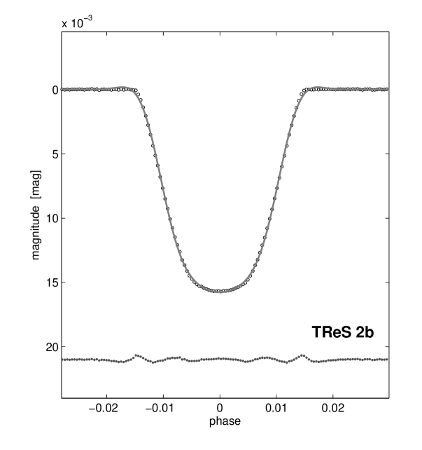
Figure 1.: The Kepler light curve of an exoplanet transit in TrES-2b (Raetz et al. 2014) is represented by points while the model fit is shown by a line. The differences between the observed magnitudes and the model, magnified by a factor of 10, are shown in the lower part of the figure.

The normally occurring features of all eclipsing system light curves are two more or less symmetrical depressions caused by mutual eclipses of gravitationally bound stellar or planetary components. The model function of eclipses $F\!_{\mathrm{e}}$ can be approximated by the sum of two symmetrical analytic functions of the phase $\varphi$. We assume that the primary eclipse is centered at the phase $\varphi=0$, while the secondary eclipse (if one is present) is centered at phase $\varphi=0.5$,

$$\displaystyle F\!_{\mathrm{e}}(\varphi)=\sum_{k=1}^{n_{\mathrm{e}}}A_{k}\left[1\!+\!C_{k}\left(\frac{\varphi_{k}}{D_{k}}\right)^{2}+\!K\left(\frac{\varphi_{k}}{D_{k}}\right)^{4}\right]\left\{1\!-\!\left\{1\!-\!\exp\left[1\!-\!\cosh\left(\frac{\varphi_{k}}{D_{k}}\right)\right]\right\}^{\mathit{\Gamma}_{\!k}}\right\};$$ (2)

$$\varphi_{k}=\left[\varphi-(k-1)/2\right]-\mathrm{round}\left[\varphi-(k-1)/2\right],$$

where the summation is over the number of eclipses, $n_{\mathrm{e}}$: $n_{\mathrm{e}}=2$ or $n_{\mathrm{e}}=1$ (the common situation for exoplanet transits), $\varphi_{k}$ are the auxiliary phases defined in the interval $\langle-0.5,0.5\rangle$, $A_{k}$ are the central depths of eclipses in mag, $D_{k}$ is the parameter expressing half-widths of eclipses, $C_{k},K$ are the correcting parameters, $\mathit{\Gamma}_{\!k}$ parameterize the kurtosis of individual eclipses.

The fit of a transit of the exoplanet TrES2b ($n_{\mathrm{e}}=1$) observed by Kepler (see Fig. 1) (Raetz et al. 2014) utilizes five parameters: $A_{1},C_{1},K,D_{1},\mathit{\Gamma}_{1}$. However, the full description of the model monochromatic light curves with two eclipses ($n_{\mathrm{e}}=2$) would generally require nine free parameters: $A_{1,2},C_{1,2},D_{1,2},\mathit{\Gamma}_{1,2}$, and $K$. Nevertheless, the most common situations would permit a reduction to 5 parameters, $A_{1,2},C,D,\mathit{\Gamma}$, because it is usually acceptable to assume that $C_{1}\simeq C_{2}$, $K\simeq 0$, $D_{1}\simeq D_{2}$, $\mathit{\Gamma}_{1}\simeq\mathit{\Gamma}_{2}$. A detailed discussion of the properties of the eclipse model function $F\!_{\mathrm{e}}$ and its possible simplifications are given in Mikulášek (2015).

Light variations of eclipsing binaries caused by eclipses are usually modified by proximity and O’Connell effects that may be modelled by a sum of cosine and sine harmonic polynomials:

$$F\!_{\rm p}(\varphi)=\sum_{k=n_{\mathrm{e}}+1}^{n_{\mathrm{p}}+n_{\mathrm{e}}}A_{k}\cos\left[2\,\pi\,(k\!-n_{\mathrm{e}})\,\varphi\right];\quad F_{\rm c}(\varphi)=\sum_{k=n_{\mathrm{p}}+n_{\mathrm{e}}+1}^{n_{\mathrm{c}}+n_{\mathrm{p}}+n_{\mathrm{e}}}A_{k}\,\sin(2\,\pi\,\varphi),$$ (3)

where $k=n_{\mathrm{e}}+1,n_{\mathrm{e}}+2,\ldots,(n_{\mathrm{e}}+n_{\mathrm{p}}+n_{\mathrm{c}})$, $n_{\mathrm{p}}$ is the number of terms in $F\!_{\rm p}(\varphi_{1})$: $n_{\mathrm{p}}=0,2,3,\ldots$, $n_{\mathrm{c}}=0$ if the O’Connell asymmetry is not present, else $n_{\mathrm{c}}=1$ (for more information see Mikulášek 2015).

The uncommon $V$ light curve of eclipsing binary V477 Lyr (see Fig. 2) is determined by 8 parameters: $A_{1,2,3,4,5},D,C,\mathit{\Gamma}$, $n_{\mathrm{p}}=3,\,n_{\mathrm{c}}=0$.

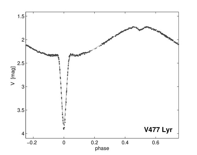
Figure 2.: $V$ light curve of an unusual eclipsing binary V477 Lyr consisting of a very hot nucleus of a planetary nebula and solar type star. Only eight free parameters is needed for the fit of the light curve strongly affected by proximity effects. $V$ data taken from Pollacco & Bell (1994).

3 Multicolour Light Curves of Exoplanet Transits and Eclipsing Binaries

The parameters of the above defined model functions, especially the amplitudes $A_{k}(\lambda)$, and parameters $C_{k}(\lambda)$, $D(\lambda),$ and $\mathit{\Gamma}(\lambda)$ are generally wavelength dependent.

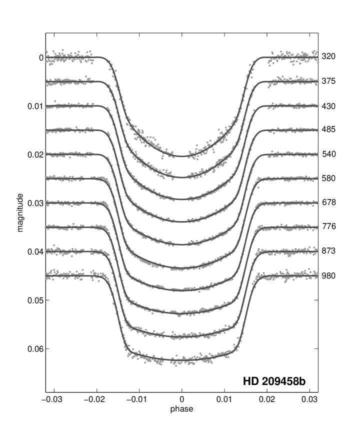
Figure 3.: Light curves of the 10-colour photometry of the exoplanet transit of HD 209458b. Effective wavelengths of individual colours are in nm. The data were taken from Knutson et al. (2007)

It follows both from the theory and experience that most of the wavelength dependencies can be well approximated by the low order polynomials of the quantity $\mathit{\Lambda}$; $\mathit{\Lambda}=\lambda_{0}/\lambda_{\mathrm{eff}}-1$, where $\lambda_{\mathrm{eff}}$ is the effective wavelength of corresponding passband, $\lambda_{0}$ is an arbitrarily selected central wavelength of the data set. Then:

$$A_{k}=\sum_{j=1}^{g_{{ak}}}a_{kj}\,\mathit{\Lambda}^{j-1},\ \ C_{l}=\sum_{j=1}^{g_{\mathrm{c}l}}c_{lj}\,\mathit{\Lambda}^{j-1},\ \ D=\sum_{j=1}^{g_{d}}d_{\!j}\,\mathit{\Lambda}^{j-1},\ \ \mathit{\Gamma}=\sum_{j=1}^{g_{\gamma}}\gamma_{k}\,\mathit{\Lambda}^{j-1},$$ (4)

where $g_{ak},g_{cl},g_{d},g_{\gamma}$, $l=1,2$ or $l=1$, are the numbers of degrees of freedom of the corresponding parameters of the model. The standard set of the monochromatic light curve model parameters of eclipsing binaries (see Sec. 2): $\{A_{k},C_{l},D,\mathit{\Gamma}\}$ can be considered as the special case of the multicolour decomposition Eq. 4: $\{a_{k1},c_{l1},d_{1},\mathit{\gamma}_{1}\}$.

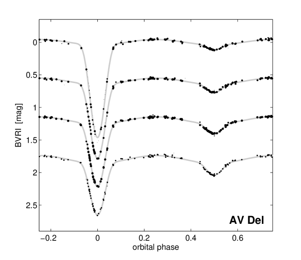
Figure 4.: BVRI light curves of a ‘cool Algol’ AV Del, consisting of a main sequence F type primary and the K subgiant filling its Roche lobe, can be approximated by our model function with 9 free parameters. The data were taken from Mader et al. (2005).

All needed parameters and their uncertainties can be determined using the standard non-linear weighted least square technique (see in Mikulášek 2015).

4 Conclusions

The outlined phenomenological modeling of eclipse-binary and planetary-transit light curves has an advantage of high efficiency and simplicity and thus can be used for a wide range of applications.

Acknowledgments

The study is supported by the grant of Ministry of Education of the Czech Republic LH14300.

References

- Hadrava (2004) Hadrava P. 2004, Publ. Astron. Inst. Czechosl. Acad. Sci., 92, 1
- Knutson et al. (2007) Knutson H. A., Charbonneau D., Noyes, R. W. et al. 2007, ApJ, 655, 564
- Mader et al. (2005) Mader J. A., Torres, G., Marschall L. A., & Rizvi A. 2005, AJ, 130, 234
- Mikulášek & Zejda, (2013) Mikulášek Z. & Zejda M., in Úvod do studia proměnných hvězd, ISBN 978-80-210-6241-2, Masaryk University, Brno 2013
- Mikulášek et al. (2008) Mikulášek Z., Krtička J., Henry G. W., Zverko J., Žižňovský et al. 2008, A&A, 485, 585
- Mikulášek (2015) Mikulášek Z. 2015, A&A, submitted
- Pollacco & Bell (1994) Pollaco D. L. & Bell S. A. 1994, MNRAS, 267, 452
- Prša & Zwitter (2005) Prša A., & Zwitter T. 2005, ApJ, 628, 426
- Prsa et al. (2011) Prsa, A., Matijevic, G., Latkovic, O. et al. 2011, Astrophysics Source Code Library, 6002
- Raetz et al. (2014) Raetz S., Maciejewski G., Ginski C., Mugrauer M. et al. 2014, MNRAS, 444, 1351
- Wilson & Devinney (1971) Wilson R. E., & Devinney, E. J. 1971, ApJ, 166, 605
- Wilson & Van Hamme (2014) Wilson R. E., & Van Hamme W. 2014, ApJ, 780, 151