GPU accelerated image reconstruction in a two-strip J-PET tomograph

Abstract

We present a fast GPU implementation of the image reconstruction routine, for a novel two strip PET detector that relies solely on the time of flight measurements.

87.57.nf, 87.57.uk

1 Introduction

In this paper we present a GPU implementation of list-mode reconstruction algorithm of a 2D strip PET. This detector consists of two parallel bars (strips) of scintillator with a photomultiplier attached to each end [1, 2].

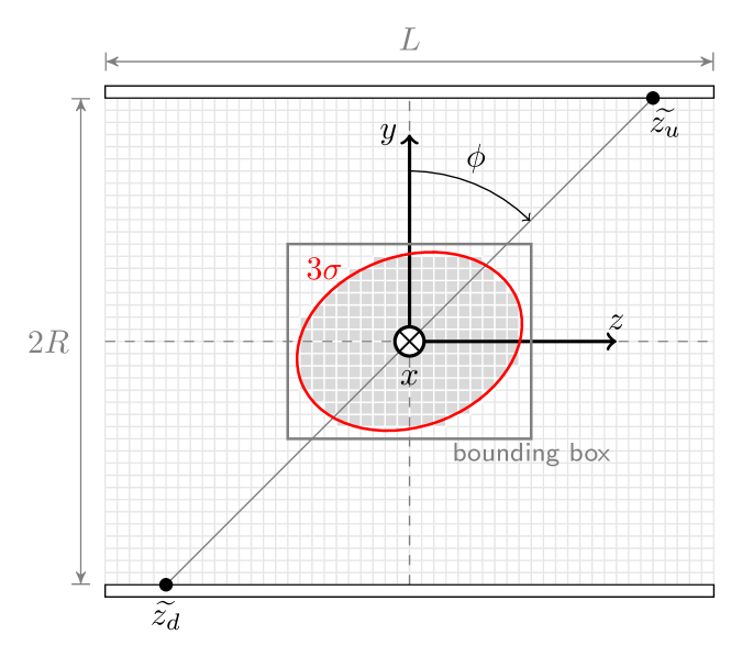
Figure 1: 2D-strip detector geometry.

By measuring the time of the arrivals of photons to each of the photomultipliers we can reconstruct the position at which $\gamma$ quanta have interacted with the scintillators as well as the position along the line-of-response (LOR) (see Figure 1). Application of the state of the art electronics developed at the Jagiellonian University allowed to achieve the required resolution [3, 4].

A double-strip prototype can be regarded as an elementary part of the full 3D “J-PET” detector under construction at our faculty[1, 2, 5, 6, 7]. The detector will consists of cylindrically arranged scintillator strips (as shown schematically in figure 2) enabling a full 3D reconstruction. However, the two strip prototype is also of interest as a cheap scanning device.

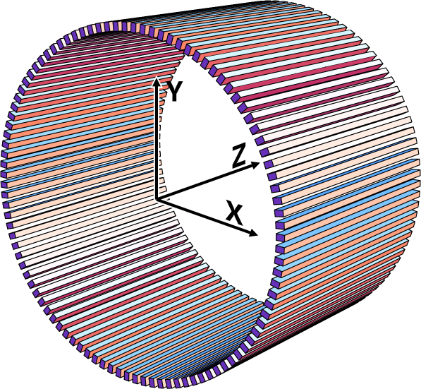
Figure 2: An example of the possible 3D detector geometry of the J-PET detector.

2 Setup

The description of the readout system electronics is beyond the scope of this paper, we will just assume that for each event we are given three numbers $(\widetilde{z_{u}},\widetilde{z_{d}},\Delta\widetilde{l})$ (see Fig. 1). By convention we use the tilde to denote measured quantities as opposite to ”real” or exact values. The $\widetilde{z_{u}}$ and $\widetilde{z_{d}}$ denote respectively the reconstructed position along the upper and lower strip and $\Delta\widetilde{l}$ is the difference of the distances along the LOR from the emission point to the upper and lower strips

$$\begin{split}\Delta\widetilde{l}&=\sqrt{(R-\widetilde{e}_{y})^{2}+(\widetilde{z_{u}}-\widetilde{e}_{z})^{2}}\\ &\phantom{=}-\sqrt{(R+\widetilde{e}_{y})^{2}+(\widetilde{z_{d}}-\widetilde{e}_{z})^{2}}.\end{split}$$ (1)

From those measurements the emission position and angle can be reconstructed directly

$$\tan\widetilde{\theta} =\frac{\widetilde{z_{u}}-\widetilde{z_{d}}}{2\bar{R}}$$ (2)

$$\widetilde{y} =-\frac{1}{2}\frac{\Delta\widetilde{l}}{\sqrt{1+\tan^{2}\widetilde{\theta}}}=\frac{2\bar{R}\Delta\widetilde{l}}{\sqrt{\widetilde{z_{u}}-\widetilde{z_{d}}+4\bar{R}^{2}}}$$

$$\widetilde{z} =\frac{1}{2}\left(\widetilde{z_{u}}+\widetilde{z_{d}}+2y\tan\widetilde{\theta}\right)$$

$$=\frac{1}{2}\left(\widetilde{z_{u}}+\widetilde{z_{d}}+\frac{(\widetilde{z_{u}}-\widetilde{z_{d}})\Delta\widetilde{l}}{\sqrt{\widetilde{z_{u}}-\widetilde{z_{d}}+4\bar{R}^{2}}}\right).$$

It is however subject to measurement errors (see the correlation matrix description at the end of Section 3). In figure 4b we present results of such direct reconstruction of the phantom depicted in the figure 4a. It is clear that the resolution of the detector is not sufficient for direct reconstruction and statistical reconstruction methods need to be applied.

The statistical reconstruction is done iteratively using the List-Mode version of the Maximal Likelihood Expectation Maximization (MLEM) algorithm. Each iteration of this algorithm defined by the following formula [8]

$$\rho(l)^{(t+1)}=\sum_{j=1}^{N}\frac{P(\widetilde{\textbf{e}}_{j}|l)\rho(l)^{(t)}}{\sum\limits_{i=1}^{M}P(\widetilde{\textbf{e}}_{j}|i)s(i)\rho(i)^{(t)}}.$$ (3)

The $\rho(l)$ is the sought tracer emission density given as the average number of emissions from pixel $l$ during the examination. The $P(\widetilde{\textbf{e}}|i)$ is a reconstruction kernel that represents the probability that an event originating in pixel $i$ will be detected as $\widetilde{\textbf{e}}$. The $s(i)$ is the sensitivity of the pixel $i$ i.e. the probability that an event emitted from pixel $i$ will be detected at all. This sensitivity can be easily calculated from the geometry:

$$\begin{split}s(y,z)&=\pi^{-1}\biggl{(}\arctan\min\biggl{(}\frac{\frac{1}{2}L-z}{R-y},\frac{\frac{1}{2}L+z}{R+y}\biggr{)}\\ &\phantom{=-\pi^{-1}}-\arctan\max\biggl{(}-\frac{\frac{1}{2}L+z}{R-y},\frac{-\frac{1}{2}L+z}{R+y}\biggr{)}\biggr{)}.\end{split}$$ (4)

In derivation have assumed the detection probability along the strip is constant and that it does not depend on the angle of incidence. This conditions should be approximately fulfilled for incidence angles not exceeding $30^{\circ}$.

The formula (3) can be rewritten as

$$\rho^{\prime}(l)^{(t+1)}=\sum_{j=1}^{N}\frac{P(\widetilde{\textbf{e}}_{j}|l)\rho^{\prime}(l)^{(t)}}{\sum\limits_{i=1}^{M}P(\widetilde{\textbf{e}}_{j}|i)\rho^{\prime}(i)^{(t)}}.$$ (5)

with

$$\rho^{\prime}(i)\equiv s(i)\rho(i).$$ (6)

In the following we will give the results of the reconstruction of $\rho^{\prime}(i)$.

The sum over $j$ in (5) runs over all collected events $\{\widetilde{e}_{j}\}$. Considering that up to hundred millions of events can be collected during a single scan this is a very time consuming calculation so the efficient calculation of the kernel $P$ is essential.

3 Kernel and correlation matrix

In [9, 10] we have found analytical approximation of $P(\widetilde{\textbf{e}}|i)$ given by

$$\begin{split}P(\widetilde{\textbf{e}}|i)&\approx\frac{\det^{\frac{1}{2}}C}{2\pi\sqrt{\vec{a}C^{-1}\vec{a}+2\vec{o}C^{-1}\vec{b}}}\\ &\phantom{\approx}\exp\left(-\frac{1}{2}\left(\vec{b}C^{-1}\vec{b}-\frac{\left(\vec{b}C^{-1}\vec{a}\right)^{2}}{\vec{a}C^{-1}\vec{a}+2\vec{o}C^{-1}\vec{b}}\right)\right)\end{split}$$ (7)

The $\vec{o}$, $\vec{a}$, $\vec{b}$ are defined as follows

$$\vec{o} =\begin{pmatrix}-(\Delta y+\widetilde{y}-R)\tan\widetilde{\theta}\cos^{-2}\widetilde{\theta}\\ -(\Delta y+\widetilde{y}+R)\tan\widetilde{\theta}\cos^{-2}\widetilde{\theta}\\ -(\Delta y+\widetilde{y})\cos^{-1}\widetilde{\theta}(1+2\tan^{2}\widetilde{\theta})\end{pmatrix},$$ (8)

$$\vec{a} =\begin{pmatrix}-(\Delta y+\widetilde{y}-R)\cos^{-2}\widetilde{\theta}\\ -(\Delta y+\widetilde{y}+R)\cos^{-2}\widetilde{\theta}\\ -(\Delta y+\widetilde{y})\cos^{-1}\widetilde{\theta}\tan\widetilde{\theta}\end{pmatrix},$$ (9)

$$\vec{b} =\begin{pmatrix}\Delta z-\Delta y\tan\widetilde{\theta}\\ \Delta z-\Delta y\tan\widetilde{\theta}\\ -2\Delta y\cos^{-1}\widetilde{\theta}\end{pmatrix}$$ (10)

and

$$\Delta y=y-\widetilde{y}\quad\text{and}\quad\Delta z=z-\widetilde{z}.$$ (11)

The $\widetilde{y}$ and $\widetilde{z}$ are the coordinates of the reconstructed emission point and $\widetilde{\theta}$ is the reconstructed emission angle of the event $\widetilde{\textbf{e}}$. The $y$ and $z$ are the coordinates of the center of pixel $i$. $C$ is the correlation matrix which in general can be of the form:

$$C^{-1}=\begin{pmatrix}\frac{1}{\sigma_{z}^{2}}&0&\gamma\\ 0&\frac{1}{\sigma_{z}^{2}}&-\gamma\\ \gamma&-\gamma&\frac{1}{\sigma_{\Delta l}^{2}}\end{pmatrix}.$$ (12)

This matrix depends on the $\widetilde{z_{u}}$ and $\widetilde{z_{d}}$. For $\sigma_{z}$. Experimentally we have found this dependence to be quite weak on the order of 10% from the center (lowest) to the edge (highest). We have found out that coefficient $\gamma$ can be neglected as long as we do not take into account events with $z_{u(d)}$ near the edge of the scintillators. This may change when we consider the full detector with longer (500mm) scintillator strips, but in this contribution we assume correlation matrix to be diagonal. Currently we achieve $\sigma_{z}\approx 10mm$ and $\sigma_{\Delta l}\approx 40mm$. Please note that the last number corresponds to $20mm$ error for the position along the emission line as the distance from the line midpoint is equal to $\frac{1}{2}\Delta l$.

Formula (7) is, at least for the range of parameters we have studied, strongly dominated by the gaussian term $\vec{b}C^{-1}\vec{b}$. This term defines an $3\sigma$ ellipse (see figure 1). For practical purposes we can assume that the kernel is zero outside this ellipse. As it is easier to work with rectangular shapes we also define a bounding box consisting of an rectangle that is circumscribed on the ellipse (see Appendix B).

4 Implementation

The iteration step described by formula (3) can be implemented as described by the pseudocode in Listing 1.

⬇

1for (auto p_l : pixels) {

2 rho_new[p_l] = 0.0;

3}

4for (auto e_j : events) {

5 auto denominator = 0.0;

6 for (auto i : ellipse(e_j)) {

7 kernel[i] = p(e_j, i);

8 denominator += kernel[i] * rho[i];

9 }

10 for (auto i : ellipse(e_j)) {

11 rho_new[i] += rho[l] * kernel[i] / denominator;

12 }

13}

Listing 1: Implementation of the reconstruction iteration routine.

Loops for(auto i : ellipse(e_j)) on lines $6$ and $10$ iterate over all pixels in the $3\sigma$ ellipse of the event $\widetilde{\textbf{e}}$. To calculate pixels contributing to this ellipse we first need to determine its bounding box in pixel space. Once bounding box is calculated we loop only trough pixels inside this bounding box. Each pixel is then tested if its center point resides inside or outside of the ellipse. Only then the whole kernel is calculated. The results are cached and used subsequently in the second loop.

4.1 CPU

The CPU implementation follows essentially the algorithm from listing 1. We use OpenMP to parallelize the outer loop (line 5) over the events. Each thread writes to its own copy of rho_new array which are added at the end of the iteration. Currently we do not take direct advantage of the AVX/SSE instruction set aside of automatic vectorization provided by Intel C++ Compiler.

4.2 GPU implementation

Next step was a naive GPU implementation based on our reference CPU implementation where each thread processes all pixels of single event, so few thousands of events are processed simultaneously by hardware threads.

Such approach has however serious drawback on GPU hardware, which is essentially a vector computer. On the NVIDIA CUDA architecture that we use, the threads are collected in batches of 32 threads called warps. All threads in a warp must execute same instruction in parallel (SIMD). In the naive implementation each thread is processing a different events with different number of pixels. That amounts to a double loop with loops bounds different across the threads of a warp. This leads to severe thread divergence and as we have discovered carries a much higher penalty then naively expected. One would expect that the execution time of a warp, would be approximately the time needed to execute the longest loops, but as it turned out it is much higher. Additionally we cannot cache visited pixels and their kernel results since it is not enough registers or shared memory to store such information given each thread processes separate event.

We can circumvent that using different pixel calculation scheduling where whole warp of 32 threads calculates a single event. This is called by us warp granularity (see Figure 3). As each thread in a warp process a single pixel from the same event there is no divergence. Different events are processed by different warps which can run independently. This algorithm also lets us better leverage available shared memory and registers. However, processor cycles are still wasted by the threads that fail the bounding ellipse test.

First it has to be noted that single event is calculated in two passes. First we need to calculate denominator of (3). This pass needs bounding box to be calculated first, then each pixel in this pass is tested with 3-sigma ellipse equation.

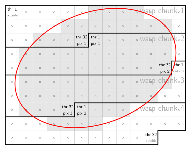
Figure 3: Warp granularity (whole event processed by single warp)

During first pass warp granularity gives us opportunity to cache visited pixels and kernel (7) in shared memory and registers, so the second pass can loop only through visited already pixels without a need to test them for ellipse inclusion. Also we can cache kernel results in registers, since each thread in warp is likely to visit just few pixels of single event.

Calculation of the denominator requires adding the contributions from the 32 threads of the warp. We have done this using the new shuffle instructions introduced in Kepler architecture. This gave a notable performance boost over standard reduction algorithm using shared memory[11].

Final optimization is to access $\rho$ (previous iteration image buffer) as texture. This produces noticeable performance boost by using hardware GPU texture unit cache and special 2D access optimized memory layout. However it can be observed that memory access still takes around $35\%$ of overall iteration time after optimizations.

5 Benchmarks and results

We have benchmarked our GPU implementation on NVIDIA GeForce GTX 770 commodity card with 4GB memory and compute capability 3.0 using CUDA SDK $6.5$, CPU implementation on Intel Xeon CPU E5-1650 v2 @ $3.50$GHz with 6 cores using ICC $15.0.0$ (Intel Composer XE $2015$). The benchmark results are presented in Table 1, while the results of reconstruction of the phantom after different number of iterations are presented in the figures 4c to 4f.

Number of Events	CPU OpenMP	GPU Thread	GPU Warp	Speedup CPU/Warp
$10$$\times 10^{6}$	$11.83$ s	$0.69$ s	$0.47$ s	$25$$\times$
$20$$\times 10^{6}$	$23.65$ s	$1.38$ s	$0.93$ s	$25$$\times$
$30$$\times 10^{6}$	$35.46$ s	$2.07$ s	$1.40$ s	$25$$\times$
$40$$\times 10^{6}$	$47.20$ s	$2.75$ s	$1.86$ s	$25$$\times$
$50$$\times 10^{6}$	$58.99$ s	$3.44$ s	$2.33$ s	$25$$\times$
$60$$\times 10^{6}$	$70.82$ s	$4.13$ s	$2.80$ s	$25$$\times$
$70$$\times 10^{6}$	$82.73$ s	$4.82$ s	$3.26$ s	$25$$\times$
$80$$\times 10^{6}$	$94.41$ s	$5.50$ s	$3.73$ s	$25$$\times$
$90$$\times 10^{6}$	$106.15$ s	$6.19$ s	$4.19$ s	$25$$\times$
$100$$\times 10^{6}$	$118.04$ s	$6.88$ s	$4.66$ s	$25$$\times$

Table 1: Single iteration reconstruction time per number of events.

(a) Ideal reconstruction

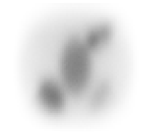
(b) Direct reconstruction

(c) after 1 iteration

(d) after 5 iterations

(e) after 10 iterations

(f) after 25 iterations

Figure 4: Phantom used in reconstruction. ($R=130$mm, $L=300$mm and $4\times 4$mm pixel size)

6 Summary and outlook

We have implemented and tested our reconstruction kernel on simulated data using realistic parameters obtained from experimental measurements. As seen from the figures 4c to 4f the results are very encouraging, considering the simplicity and the resolution of our setup. Implementing the reconstruction algorithm on the commodity GPU provided a 25-fold speedup that allows real-time processing. One should note however that this speed is partly due to not taking advantage of the CPU vector AVX instruction set. The reason for this is that as we have already pointed out in [12] the CUDA and OpenCL programming model is inherently vectorized while CPU is still viewed as superscalar processor with vector instructions mixed in. This is only now slowly changing with introduction of new compiler pragmas to deal explicitly with vectorization in a similar way as OpenMP deals with parallelization.

In derivation of the (7) we have assumed a very simple detector geometry with scintillators approximated by thin lines. In reality they have a rectangular cross section of 5x20$mm^{2}$. To some extent this was taken into account by using the errors estimated from real scintillators. The model however must be validated on real data (which is already collected) and this is a subject of an ongoing investigation.

Appendix A Phantom

Phantom definition is given in table 2. Each row corresponds to an ellipse with center $(x,y)$ the half-axes $a$ and $b$ rotated by angle $\phi$ counter-clockwise. The $\rho$ denotes the relative density of the tracer. When two ellipses overlap the $\rho$ is taken from the topmost (in table) one.

x	y	a	b	$\phi$	$\rho$
0	0	30	60	0	0.3
50	-62	10	33	-40	0.3
-50	-63	20	33	45	0.5
60	65	13	14	0	0.5
35	55	12	12	0	0.7
0	0	120	110	0	0.1

Table 2: Phantom description.

Appendix B Bounding box

Given an ellipse defined by the equation

$$Ay^{2}+Cyz+Bz^{2}=R^{2}$$ (13)

its bounding box is a rectangle with lower left corner at

$$y=-\frac{R}{\sqrt{A-\frac{C^{2}}{B}}},\qquad z=-\frac{R}{\sqrt{B-\frac{C^{2}}{A}}}$$ (14)

and symmetric upper right corner. This combined with

$$\begin{split}\vec{b}C^{-1}\vec{b}&=2\frac{(\Delta z-\Delta y\tan\widetilde{\theta})^{2}}{\sigma_{z}^{2}}+4\frac{\Delta y^{2}}{\sigma_{\Delta l}^{2}cos^{2}\widetilde{\theta}}\\ &=\Delta z^{2}\frac{2}{\sigma_{z}^{2}}-2\Delta z\Delta y\frac{2\tan\widetilde{\theta}}{\sigma_{z}^{2}}\\ &\phantom{=\Delta z^{2}}+\Delta y^{2}\left(\frac{2\tan^{2}\widetilde{\theta}}{\sigma_{z}^{2}}+\frac{4}{\sigma_{\Delta l}^{2}\cos^{2}\widetilde{\theta}}\right)\end{split}$$ (15)

allows us to calculate the bounding box of the $3\sigma$ ellipse for each event.

References

- [1] P. Moskal et al., Nucl. Instrum. Meth. A 764, 317 (2014) [arXiv:1407.7395 [physics.ins-det]].
- [2] P. Moskal et al., Nuclear Inst. and Methods in Physics Research A 775 (2015), pp. 54-62 [arXiv:1412.6963 [physics.ins-det]].
- [3] M. Pałka et al., Bio-Algorithms and Med-Systems 10, 41-45 (2014); [arXiv:1311.6127 [physics.ins-det]]
- [4] G. Korcyl et al., Bio-Algorithms and Med-Systems 10, 37-40 (2014)
- [5] L. Raczyński et al., Nucl. Instrum. Meth. A 764, 186 (2014) [arXiv:1407.8293 [physics.ins-det]].
- [6] P. Moskal et al., Nuclear Med. Rev. C 15, 81-84 (2012); e-print arXiv:1305.5559.
- [7] P. Moskal et al., Nuclear Med. Rev. C 15, 68-69 (2012); e-print arXiv:1305.5562.
- [8] L. Parra and H.H. Berret, IEEE Trans. Med. Imaging, 17, 228–235 (1998).
- [9] P. Białas, J. Kowal, A. Strzelecki et al., Acta Phys. Polon. B Proceed. Suppl. 6, 1027-1036 (2013); e-print arXiv:1310.1614.
- [10] P. Białas, J. Kowal, A. Strzelecki et al., Bio-Algorithms and Med-Systems 2014; 10(1): 9–12.
- [11] M. Harris ”Optimizing parallel reduction in CUDA”, http://docs.nvidia.com/cuda/samples/6_Advanced/reduction/doc/ reduction.pdf
- [12] P. Bialas, J. Kowal, A. Strzelecki, Computing and Informatics 33, 1001-1008, (2014).