Entropic uncertainty relations and topological-band insulator transitions in 2D gapped Dirac materials

Abstract

Uncertainty relations are studied for a characterization of topological-band insulator transitions in 2D gapped Dirac materials isoestructural with graphene. We show that the relative or Kullback-Leibler entropy in position and momentum spaces, and the standard variance-based uncertainty relation give sharp signatures of topological phase transitions in these systems.

1 Introduction

Recently, there is a growing interest in the study of 2D gapped Dirac materials isoestructural with graphene. One of these materials is silicene, which is a two dimensional crystal of silicon, with a relevant intrinsic spin-orbit coupling (as compared to graphene), studied theoretically [1, 2] and experimentally [3, 4, 5, 6, 7]. Other gapped Dirac materials are germanene, stannene and Pb [8]. For these systems, the low energy electronic properties can be described by a Dirac Hamiltonian, like in graphene, but the electrons are massive due to the relative large spin-orbit coupling $\Delta_{\mathrm{so}}$. In fact, we will consider the application of a perpendicular electric field $\mathcal{E}_{z}=\Delta_{z}/l$ ($l$ is the inter-lattice distance of the buckled honeycomb structure) to the material sheet, which generates a tunable band gap $|\Delta_{s\xi}|=|(\Delta_{z}-s\xi\Delta_{\mathrm{so}})/2|$ ($s$ and $\xi$ denote spin and valley, respectively). There is a topological phase transition [9] from a topological insulator (TI, $|\Delta_{z}|<\Delta_{\mathrm{so}}$) to a band insulator (BI, $|\Delta_{z}|>\Delta_{\mathrm{so}}$), at a charge neutrality point (CNP) $\Delta_{z}^{(0)}=s\xi\Delta_{\mathrm{so}}$, where there is a gap cancellation between the perpendicular electric field and the spin-orbit coupling, thus exhibiting a semimetal behavior.

A 2D topological insulator was theoretically studied in [10] and first discovered experimentally in HgTe quantum wells in [11]. A TI-BI transition is characterized by a band inversion with a level crossing at some critical value of a control parameter (electric field, quantum well thickness, etc). Recently, we have found that electron-hole Wehrl entropies of a quantum state in a coherent-state representation provide a useful tool to identify TI-BI phase transitions [12].

In this work we explore the connection between the TI-BI transitions in some 2D Dirac materials with the Shannon information entropies of the wave packet probability densities in position and momentum spaces and, in particular, with the entropic uncertainty relation. The uncertainty principle can be quantified in terms of the usual variance-based uncertainty relation, $\Delta x\Delta p\geq\frac{1}{2}$, or alternatively by means of the entropic uncertainty relation [13, 14, 15] which has been shown to be more appropriate in different physical situations [16, 17, 18, 19, 20, 21, 22, 23, 25]. If we define the position and momentum densities of a state $\Psi$ as $\rho({\bf r})=|\Psi({\bf r})|^{2}$ and $\gamma({\bf p})=|\Phi({\bf p})|^{2}$, respectively, with $\Psi({\bf r})$ the position and $\Phi({\bf p})$ the momentum wave packets, the entropic uncertainty relation is given by

$$S_{\rho}+S_{\gamma}\geq D(1+\ln\pi)$$ (1)

where $D$ is the dimension of the position and momentum space and where $S_{f}=-\int f({\bf x})\ln(f({\bf x}))d{\bf x}$ is the so called Shannon information entropy of a density $f$. The equality is reached when the wave packets in position and momentum spaces are Gaussians. The Shannon information entropy measures the uncertainty in the localization of the wave packet in position or momentum spaces, so that the higher the Shannon entropy is, the smaller the localization of the wave packet is; and the smaller the entropy is, the more concentrated the wave function is. Besides we will consider the relative or Kullback-Leibler entropy to characterize the topological-band insulator transitions (see section 4) in these materials.

The paper is organized as follows. Firstly, in Section 2, we shall introduce the low energy Hamiltonian for some 2D Dirac materials (namely: silicene, germanene, stantene,…). Then, in Section 3, we will characterize topological-band insulator transitions in silicene in terms of the entropic uncertainty relation. In Section 4, the connection between the relative entropy and the topological-band insulator transitions is studied. In Section 5 we use the Heisenberg uncertainty relation to characterize the TI-BI phase transition. Finally, some concluding remarks will be given in the last Section.

2 Low energy Hamiltonian

Let us consider a monolayer silicene film with external magnetic $B$ and electric $\mathcal{E}_{z}$ fields applied perpendicular to the silicene plane. The low energy effective Hamiltonian in the vicinity of the Dirac point is given by [9]

$$H_{s}^{\xi}=v_{F}(\sigma_{x}p_{x}-\xi\sigma_{y}p_{y})-\xi s\Delta_{\mathrm{so}}\sigma_{z}+\Delta_{z}\sigma_{z},$$ (2)

where $\xi$ corresponds to the inequivalent corners ${K}$ ($\xi=1$) and ${K}^{\prime}$ ($\xi=-1$) of the Brillouin zone, respectively, ${\sigma}_{j}$ are the usual Pauli matrices, $v_{F}$ is the Fermi velocity of the Dirac fermions (see Table 1 for theoretical estimations in Si, Ge and Sn), spin up and down values are represented by $s=\pm 1$, respectively, and $\Delta_{\rm so}$ is the band gap induced by intrinsic spin-orbit interaction, which provides a mass to the Dirac fermions. We are considering the application of a constant electric field $\mathcal{E}_{z}$ which creates a potential difference $\Delta_{z}=l\mathcal{E}_{z}$ between sub-lattices. The value $l$ appears in table 1 for different materials. The values of the spin-orbit energy gap induced by the intrinsic spin-orbit coupling has been theoretically estimated [26, 27, 28, 8] for different 2D Dirac materials that we show in Table 1.

	$\Delta_{\mathrm{so}}$ (meV)	$l$ ($\AA$)	$v_{F}$ ($10^{5}$m/s)
Si	4.2	0.22	4.2
Ge	11.8	0.34	8.8
Sn	36.0	0.42	9.7
Pb	207.3	0.44	–

Table 1: Approximate values of model parameters $\Delta_{\mathrm{so}}$ (spin-orbit coupling), $l$ (interlattice distance) and $v_{F}$ (Fermi velocity) for two dimensional Si, Ge, Sn and Pb sheets. These data have been obtain from first-principles computations in [8] ($\Delta_{\mathrm{so}}$ and $l$) and [29, 30] ($v_{F}$).

The eigenvalue problem can be easily solved. Using the Landau gauge, $\vec{A}=(0,Bx,0)$, the corresponding eigenvalues and eigenvectors for the $K$ and $K^{\prime}$ points are given by [9, 31, 12]

$$E_{n}^{s\xi}=\left\{\begin{array}[]{l}\mathrm{sgn}(n)\sqrt{|n|\hbar^{2}\omega^{2}+\Delta_{s\xi}^{2}},\quad n\neq 0,\\ -\xi\Delta_{s\xi},\quad n=0,\end{array}\right.$$ (3)

and

$$|n\rangle_{s\xi}=\left(\begin{array}[]{c}-iA_{n}^{s\xi}||n|-\xi_{+}\rangle\\ B_{n}^{s\xi}||n|-\xi_{-}\rangle\end{array}\right),$$ (4)

where we denote by $\xi_{\pm}=(1\pm\xi)/2$, the Landau level index $n=0,\pm 1,\pm 2,\dots$, the cyclotron frequency $\omega=v_{F}\sqrt{2eB/\hbar}$, the lowest band gap $\Delta_{s\xi}\equiv(\Delta_{z}-s\xi\Delta_{\mathrm{so}})/2$ and the constants $A_{n}^{s\xi}$ and $B_{n}^{s\xi}$ are given by [31]

$$A_{n}^{s\xi} = \left\{\begin{array}[]{l}\mathrm{sgn}(n)\sqrt{\frac{|E_{n}^{s\xi}|+\mathrm{sgn}(n)\Delta_{s\xi}}{{2|E_{n}^{s\xi}|}}},\quad n\neq 0,\\ \xi_{-},\quad n=0,\end{array}\right.$$ (7)

$$B_{n}^{s\xi} = \left\{\begin{array}[]{l}\sqrt{\frac{|E_{n}^{s\xi}|-\mathrm{sgn}(n)\Delta_{s\xi}}{{2|E_{n}^{s\xi}|}}},\quad n\neq 0,\\ \xi_{+},\quad n=0,\end{array}\right.$$ (10)

The vector $||n|\rangle$ denotes an orthonormal Fock state of the harmonic oscillator.

We will do all the numerical analysis in silicene but the results will be valid just replacing the corresponding parameters in Table 1.

As already stated, there is a prediction (see e.g. [26, 27, 28, 32]) that when the gap $|\Delta_{s\xi}|$ vanishes at the CNP $\Delta_{z}^{(0)}$, silicene undergoes a phase transition from a topological insulator (TI, $|\Delta_{z}|<\Delta_{\mathrm{so}}$) to a band insulator (BI, $|\Delta_{z}|>\Delta_{\mathrm{so}}$). This topological phase transition entails an energy band inversion. Indeed, in Figure 1 we show the low energy spectra 3 as a function of the external electric potential $\Delta_{z}$ for $B=0.05$ T. One can see that there is a band inversion for the $n=0$ Landau level (either for spin up and down) at both valleys. The energies $E_{0}^{1,\xi}$ and $E_{0}^{-1,\xi}$ have the same sign in the BI phase and different sign in the TI phase, thus distinguishing both regimes. We will observe a similar “inversion” behavior in entropic and variance-based uncertainty relations for the Hamiltonian eigenstates 4, thus providing a quantum-information characterization of the topological phase transition.

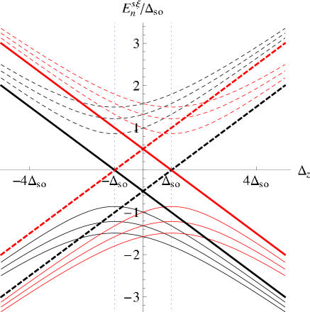
Figure 1: Low energy spectra of silicene as a function of the external electric potential $\Delta_{z}$ for $B=0.05$ T. Landau levels $n=\pm 1,\pm 2$ and $\pm 3$, at valley $\xi=1$, are represented by dashed (electrons) and solid (holes) thin lines, black for $s=-1$ and red for $s=1$ (for the other valley we simply have $E_{n}^{s,-\xi}=E_{n}^{-s,\xi}$). The lowest Landau level $n=0$ is represented by thick lines at both valleys: solid at $\xi=1$ and dashed at $\xi=-1$. Vertical blue dotted grid lines indicate the CNPs separating BI ($|\Delta_{z}|>\Delta_{\mathrm{so}}$) from TI ( $|\Delta_{z}|<\Delta_{\mathrm{so}}$) phases.

3 Entropic uncertainty relation and topological phase transition

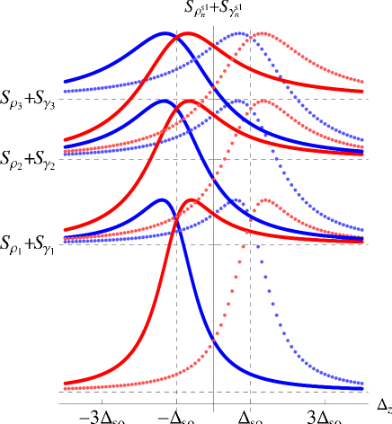
Figure 2: Entropic uncertainty relation $S_{\rho_{n}^{s1}}+S_{\gamma_{n}^{s1}}$ as a function of the electric potential $\Delta_{z}$ for the Landau levels: $n=\pm 1,\pm 2$ and $\pm 3$ (electrons in blue and holes in red), with spin up (dotted lines) and down (solid lines) and magnetic field $B=0.01$T at valley $\xi=1$. Electron and hole entropy curves cross at the critical value of the electric potential $\Delta_{z}^{(0)}=-s\Delta_{\mathrm{so}}$ (vertical black dotted grid lines indicate this CNPs), $S_{\rho_{|n|}}+S_{\gamma_{|n|}}$ are the asymptotic values for $\Delta_{z}\rightarrow\pm\infty$ (horizontal black dotted grid lines).

In order to compute Shannon entropies, firstly we have to write the Hamiltonian eigenstates 4 in position and momentum representation. We know that Fock (number) states $|n\rangle$ can be written in position and momentum representation as

$$\langle x|n\rangle=\frac{\omega^{1/4}}{\sqrt{2^{n}n!\sqrt{\pi}}}e^{-\omega x^{2}/2}H_{n}\left(\sqrt{\omega}x\right)$$ (11)

$$\langle p|n\rangle=\frac{(-i)^{n}}{\sqrt{2^{n}n!\sqrt{\omega\pi}}}e^{-p^{2}/2\omega}H_{n}\left(p/\sqrt{\omega}\right)$$ (12)

where $H_{n}(x)$ are the Hermite polynomials of degree $n$. We will introduce the number-state densities in position and momentum spaces as $\rho_{n}(x)=|\langle x|n\rangle|^{2}$ and $\gamma_{n}(x)=|\langle p|n\rangle|^{2}$, which are normalized according to $\int\rho_{n}(x)dx=1$ and $\int\gamma_{n}(x)dx=1$. Now, taking into account Eq. (4), the position and momentum densities for the Hamiltonian eigenvectors 4 are given, respectively, by

$$\rho_{n}^{s\xi}(x)=(A_{n}^{s\xi})^{2}|\langle x||n|-\xi_{+}\rangle_{s\xi}|^{2}+(B_{n}^{s\xi})^{2}|\langle x||n|-\xi_{-}\rangle_{s\xi}|^{2}$$ (13)

$$\gamma_{n}^{s\xi}(p)=(A_{n}^{s\xi})^{2}|\langle p||n|-\xi_{+}\rangle_{s\xi}|^{2}+(B_{n}^{s\xi})^{2}|\langle p||n|-\xi_{-}\rangle_{s\xi}|^{2}.$$ (14)

We will study the position and momentum entropies

$$S_{\rho_{n}^{s\xi}}\equiv-\int_{-\infty}^{\infty}\rho_{n}^{s\xi}(x)\ln\left(\rho_{n}^{s\xi}(x)\right)dx$$ (15)

$$S_{\gamma_{n}^{s\xi}}\equiv-\int_{-\infty}^{\infty}\gamma_{n}^{s\xi}(p)\ln\left(\gamma_{n}^{s\xi}(p)\right)dp.$$ (16)

If we make a change of variable, it is straightforward to see that $S_{\rho_{n}^{s\xi}}=S_{\gamma_{n}^{s\xi}}-\ln\left(\omega\right)$.

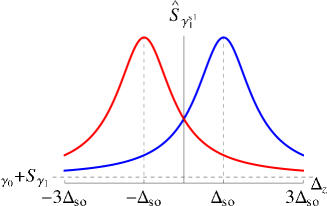
Figure 3: Combined Shannon entropies 17 and 18 of electron plus holes for $n=1$, in position and momentum spaces, $\hat{S}_{\rho_{n}^{s1}}$ (left) and $\hat{S}_{\gamma_{n}^{s1}}$ (right), respectively, as a function of the electric potential $\Delta_{z}$, for $B=0.01$T, with spin up (blue) and down (red) and valley $\xi=1$. The combined entropies have a maximum at the critical value of the electric potential $\Delta_{z}^{(0)}=-s\Delta_{\mathrm{so}}$ (vertical dashed grid lines indicate these CNPs).

In figure 2 we plot $S_{\rho_{n}^{s\xi}}+S_{\gamma_{n}^{s\xi}}$ as a function of the external electric potential $\Delta_{z}$ for the Landau levels: $n=\pm 1,\pm 2$ and $\pm 3$ (electrons in blue and holes in red), with spin up (dotted lines) and down (solid lines) and magnetic field $B=0.01$T at valley $\xi=1$. Electron-hole entropy curves cross at the CNP $|\Delta_{z}|=\Delta_{\mathrm{so}}$. For electrons (resp. holes), the asymptotic entropies in position space are given by $S_{\rho_{|n|-1}}$ (resp. $S_{\rho_{|n|}}$) for $\Delta_{z}\rightarrow\infty$ and $S_{\rho_{|n|}}$ (resp. $S_{\rho_{|n|-1}}$) for $\Delta_{z}\rightarrow-\infty$. In momentum space the behavior is analogous. The uncertainty relation has the same value for spin up (resp. down) electrons and holes at the CNP point $\Delta_{z}=\Delta_{\mathrm{so}}$ (resp. $\Delta_{z}=-\Delta_{\mathrm{so}}$). Moreover, for each $n$, note that in the BI phase the electrons (resp. holes) uncertainty goes to greater value than holes (resp. electrons) uncertainty for $\Delta_{z}<-\Delta_{\mathrm{so}}$ (resp. $\Delta_{z}>\Delta_{\mathrm{so}}$). We have checked that the smaller the magnetic field strength, the sharper this effect is.

In figure 3 we have plotted the combined entropy of electrons plus holes

$$\hat{S}_{\rho_{n}^{s1}}=S_{\rho_{n}^{s1}}+S_{\rho_{-n}^{s1}}$$ (17)

$$\hat{S}_{\gamma_{n}^{s1}}=S_{\gamma_{n}^{s1}}+S_{\gamma_{-n}^{s1}}$$ (18)

in position and momentum representation for $n=1$. We can observe that the combined entropies exhibit a maximum at the CNPs in both representation spaces. This is a common feature for general $n$.

4 Kullback-Leibler entropy

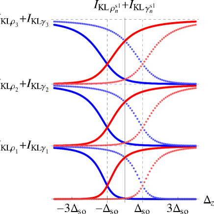
Figure 4: Kullback-Leibler uncertainty relation $I_{KL\rho_{n}^{s1}}+I_{KL\gamma_{n}^{s1}}$ as a function of the electric potential $\Delta_{z}$ for the Landau levels: $n=\pm 1,\pm 2$ and $\pm 3$ (electrons in blue and holes in red), with spin up (dotted lines) and down (solid lines) and magnetic field $B=0.01$T at valley $\xi=1$. Electron and hole entropy curves cross at the critical value of the electric potential $\Delta_{z}^{(0)}=-s\Delta_{\mathrm{so}}$ (vertical black dotted grid lines indicate this CNPs),

The relative or Kullback-Leibler entropy is a measure for the deviation of a density $f({\bf r})$ from a reference density $g({\bf r})$ [33] is defined as

$$I_{KL}(f,g)=\int f({\bf r})\ln\left(\frac{f({\bf r})}{g({\bf r})}\right)d{\bf r}$$ (19)

Recently, the relative Rényi and Kullback-Leibler entropies have been found to be an excellent marker of a quantum phase transition in the Dicke [34, 35] and in the $U(3)$ vibron model [36]. In this section we will explore the utility of the relative entropy as an indicator of a topological phase transition. For this purpose, we will consider as reference densities the position and momentum densities $\rho_{0}(x)$ and $\gamma_{0}(p)$, respectively, which are the densities for minimum uncertainty in relation (1). Therefore, we will analyze how different is a density from the minimum uncertainty density.

We will study the position and momentum entropies

$$I_{KL\rho_{n}^{s\xi}}\equiv\int_{-\infty}^{\infty}\rho_{n}^{s\xi}(x)\ln\left(\frac{\rho_{n}^{s\xi}(x)}{\rho_{0}(x)}\right)dx$$ (20)

$$I_{KL\gamma_{n}^{s\xi}}\equiv\int_{-\infty}^{\infty}\gamma_{n}^{s\xi}(p)\ln\left(\frac{\gamma_{n}^{s\xi}(p)}{\gamma_{0}(p)}\right)dp.$$ (21)

Again, it is straightforward that $I_{KL\rho_{n}^{s\xi}}=I_{KL\gamma_{n}^{s\xi}}$.

In figure 4 we plot the sum $I_{KL\rho_{n}^{s1}}+I_{KL\gamma_{n}^{s1}}$ as a function of the external electric potential $\Delta_{z}$ for the Landau levels $n=\pm 1,\pm 2$ and $\pm 3$ (electrons in blue and holes in red), with spin up (dots lines) and down (solid lines). The figure corresponds to a magnetic field $B=0.01$T. Electron-hole relative entropy curves cross at the CNP $|\Delta_{z}|=\Delta_{\mathrm{so}}$ at which they reach the values $\bar{I}_{n}^{s}\approx 0.37$, $1.96$ and $3.69$ for $|n|=$ $1$, $2$ and $3$ respectively. For electrons (resp. holes) the asymptotic entropies in position space are given by $I_{KL\rho_{|n|-1}}$ (resp. $I_{KL\rho_{|n|}}$) for $\Delta_{z}\rightarrow\infty$ and $I_{KL\rho_{|n|}}$ (resp. $I_{KL\rho_{|n|-1}}$) for $\Delta_{z}\rightarrow-\infty$. In momentum space the behavior is analogous. Note the electron-hole entropy inversion phenomenon anticipated at the end of Section 2. Indeed, the quantity $I_{KL\rho_{n}^{s1}}+I_{KL\gamma_{n}^{s1}}-\bar{I}_{n}^{s}$ has the same sign for spin up and down electrons (idem for holes) in the BI phase ($|\Delta_{z}|>\Delta_{\mathrm{so}}$) and different sign in the TI phase ($|\Delta_{z}|<\Delta_{\mathrm{so}}$).

5 Heisenberg uncertainty relation and topological phase transition

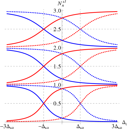
Figure 5: Expectation value of the number operator $N=a^{\dagger}a$ in the energy eigenstate $|n\rangle_{s\xi}$ as a function of the electric potential $\Delta_{z}$ for the Landau levels: $n=\pm 1,\pm 2$ and $\pm 3$ (electrons in blue and holes in red), with spin up (dotted lines) and down (solid lines) and magnetic field $B=0.01$T at valley $\xi=1$. Mean number curves cross at the critical value of the electric potential $\Delta_{z}^{(0)}=-s\Delta_{\mathrm{so}}$ (vertical black dotted grid lines indicate these CNPs), for which $N_{n}^{s\xi}=|n|/2$ (horizontal black dotted grid lines)

Entropic uncertainty relation provides a refined version of the Heisenberg uncertainty relation (see [37] and references therein):

$$\Delta x\Delta p\geq\frac{1}{2}\exp{[S_{\rho}+S_{\gamma}-1-\ln{\pi}]}\geq\frac{1}{2}.$$ (22)

It gives a stronger bound for the variance product than the standard $\frac{1}{2}$. In this section, we shall explore the more usual Heisenberg uncertainty relation.

Introducing position and momentum operators through a bosonic mode, $[a,a^{\dagger}]=1$, as usual:

$$X=\frac{1}{\sqrt{2\omega}}(a^{\dagger}+a),\;P=i\sqrt{\frac{\omega}{2}}(a^{\dagger}-a),$$ (23)

we can easily compute the expectation values of $X$ and $P$ and their fluctuations in an energy eigenstate 4 as

$$\langle n|X|n\rangle_{s\xi}=0,\;\langle n|P|n\rangle_{s\xi}=0,$$ (24)

$$\langle n|X^{2}|n\rangle_{s\xi}=\frac{1}{\omega}(N_{n}^{s\xi}+\frac{1}{2})=\frac{1}{\omega^{2}}\langle n|P^{2}|n\rangle_{s\xi},$$ (25)

where

$$N_{n}^{s\xi}=(A_{n}^{s\xi})^{2}(|n|-1)+(B_{n}^{s\xi})^{2}|n|$$ (26)

is the expectation value of the number operator $N=a^{\dagger}a$ in the energy eigenstate $|n\rangle_{s\xi}$. Therefore, the product of standard deviations, $\Delta X_{n}^{s\xi}\Delta P_{n}^{s\xi}=N_{n}^{s\xi}+\frac{1}{2}$, is written in terms of $N_{n}^{s\xi}$ solely. In Figure 5 we represent $N_{n}^{s\xi}$ as a function of the electric potential $\Delta_{z}$ for several Landau levels. We observe the same electron-hole curve inversion phenomenon as for the entropy curves. The quantity $N_{n}^{s\xi}-\frac{|n|}{2}$ has the same sign for spin up and down electrons (idem for holes) in the BI phase ($|\Delta_{z}|>\Delta_{\mathrm{so}}$) and different sign in the TI phase ($|\Delta_{z}|<\Delta_{\mathrm{so}}$).

6 Conclusions

We have explored how different quantifications of the uncertainty relation characterize a topological phase transition in a group of 2D Dirac gapped materials (monolayer sheets of Si, Ge, Sn, and Pb). Firstly we have inspected the entropic uncertainty relation. We have found that the electron-hole entropic curves cross at the charge neutrality poin (CNP), that is, the electron and holes with spin up (down) have the same uncertainty at the critical point $\Delta_{z}=\Delta_{\mathrm{so}}$ ($\Delta_{z}=-\Delta_{\mathrm{so}}$). The combined entropy of electrons plus holes shows a maximum at the critical points in position and momentum spaces; therefore, the combined electron plus hole density, for spin up (resp. down), is more delocalized at the CNP $\Delta_{z}=\Delta_{\mathrm{so}}$ (resp. $\Delta_{z}=-\Delta_{\mathrm{so}}$). Furthermore, we have analyzed the relative (or Kullback-Leibler) entropy, finding that the sum of the relative entropies in position and momentum spaces identifies each phase (band and topological insulator) at the CNPs. For completeness we have considered the product of standard deviations observing the same electron-hole uncertainty curve inversion phenomenon. Summarizing, we have related the uncertainty principle and the topological phase transitions in this model. We expect that this analysis might be applicable to other problems to obtain a general/deepest connection between both concepts: uncertainty principle and topological phase transitions.

References

- [1] K. Takeda, K. Shiraishi, Phys. Rev. B 50 (1994) 14916.
- [2] G. G. Guzman-Verri, L. Lew Yan, Phys. Rev. B 76 (2007) 075131.
- [3] P. Vogt et al., Phys. Rev. Lett. 108 (2012) 155501.
- [4] B. Augray, A. Kara, S. B. Vizzini, H. Oughaldou, C. LéAndri, B. Ealet, G. Le Lay, App. Phys. Lett. 96 (2010) 183102.
- [5] B. Lalmi, H. Oughaddou, H. Enriquez, A. Kara, S. B. Vizzini, B. N. Ealet, B. Augray, App. Phys. Letters 97 (2010) 223109.
- [6] A. Feurence, R. Friedlein, T. Ozaki, H. Kawai, Y. Wang, Y. Y. Takamura, Phys. Rev. Lett. 108 (2012) 245501.
- [7] P. E. Padova et al., App. Phys. Lett. 96 (2010) 261905.
- [8] W-F. Tsai, C-Y. Huang, T-R Chang et al. Nat. Commun. 4, 1500 (2013)
- [9] M. Tahir, U. Schwingenschlögl, Scientific Reports, 3, 1075 (2013).
- [10] Kane C L and Mele E J, Phys. Rev. Lett. 95, 226801 (2005)
- [11] B. Andrei Bernevig, Taylor L. Hughes and Shou-Cheng Zhang, Science 314, 1757-1761 (2006).
- [12] M. Calixto and E. Romera, EPL 109, 40003 (2015)
- [13] I. I. Hirschman, Am. J. Math. 79, 152 (1957)
- [14] Bialynicki-Birula, I., Mycielski, J.: Commun. Math. Phys. 44, 129 (1975)
- [15] W. Beckner, Ann. Math. 102, 159 (1975)
- [16] H. Maassen, J. B. M. Uffink, Phys. Rev. Lett. 60, 1103 (1988)
- [17] J. Sánchez-Ruiz, Phys. Lett. A 244, 189 (1998)
- [18] E. Majerníková, V. Majerník, and S. Shpyrko, Eur. Phys. J. B 38, 25 (2004).
- [19] I. Bialynicki-Birula, Phys. Rev. A 74, 052101 (2006)
- [20] E. Romera, F. de los Santos Phys. Rev. Lett.99, 263601 (2007); Phys Rev. A 78, 013837 (2008).
- [21] T. Schürmann and I. Hoffmann Found Phys 39, 958 (2009).
- [22] S. R. Gadre, Phys. Rev. A 30, 620 (1984).
- [23] S. R. Gadre, S. B. Sears, S. J. Chakrovarty and R. D. Bendale Phys. Rev. A 32, 2602 (1985).
- [24] E. Romera, M. Calixto and Á. Nagy, EPL, 97, 20011 (2012).
- [25] M. Calixto, Á. Nagy, I. Paradela and E. Romera, Phys. Rev. A 85, 053813 (2012)
- [26] N. D. Drummond, V. Zólyomi, and V. I. Fal’ko, Phys. Rev. B 85, 075423 (2012).
- [27] C. C. Liu, W. Feng, and Y. Yao, Phys. Rev. Lett. 107, 076802 (2011).
- [28] C. C. Liu, H. Jiang, and Y. Yao, Phys. Rev. B 84, 195430 (2011).
- [29] S. Trivedi, A. Srivastava and R. Kurchania, J. Comput. Theor. Nanosci. 11, 1-8 (2014). doi:10.1166/jctn.2014.3428
- [30] B van den Broek et al. 2D Materials 1 (2014) 021004. doi:10.1088/2053-1583/1/2/021004
- [31] L. Stille, C. J. Tabert, and E. J. Nicol, Phys. Rev. B 86, 195405 (2012); C.J. Tabert and E.J. Nicol, Phys. Rev. Lett. 110, 197402 (2013); C.J. Tabert and E.J. Nicol, Phys. Rev. B 88, 085434 (2013).
- [32] M. Ezawa, New Journal of Physics 14 (2012) 033003
- [33] S. Kullback and R. A. Leibler, Ann. Math. Stat. 22, 79 (1951).
- [34] E. Romera, K. Sen, Á. Nagy, J. Stat. Mech. P09016 (2011).
- [35] E. Romera and Á. Nagy, Phys. Lett. A 377, 3098 (2013).
- [36] E. Romera, M. Calixto and Á. Nagy, J. Mol. Model. 20, 2237 (2014)
- [37] J. J. Halliwell, Phys. Rev. D 48, 2739 (1993).