Comment on ”Stellar activity masquerading as planets in the habitable zone of the M dwarf Gliese 581”

Abstract

Robertson et al.(Reports, July 25 2014, p440-444)(1) claimed that activity-induced variability is responsible for the Doppler signal of the proposed planet candidate GJ 581d. We point out that their analysis using periodograms of residual data is incorrect, further promoting inadequate tools. Since the claim challenges the viability of the method to detect exo-Earths, we urge for a correct re-analysis (provided as an appendix in pre-print version).

GJ 581d was the first planet candidate of a few Earth masses reported in the circumstellar habitable zone of another star (1). It was detected by measuring the radial velocity variability of its host star using High Accuracy Radial Velocity Planet Searcher (HARPS) (1,2). Doppler time series are usually modeled as the sum of Keplerian signals plus additional effects (e.g., correlations with activity). Detecting a planet candidate consists of quantifying the improvement of a merit statistic when one signal is added to the model. Approximate methods are often used to speed up the analyses, such as computing periodograms on residual data. Even when models are linear, correlations exist between parameters. Similarly, statistics based on residual analyses are biased quantities and cannot be used for model comparison.

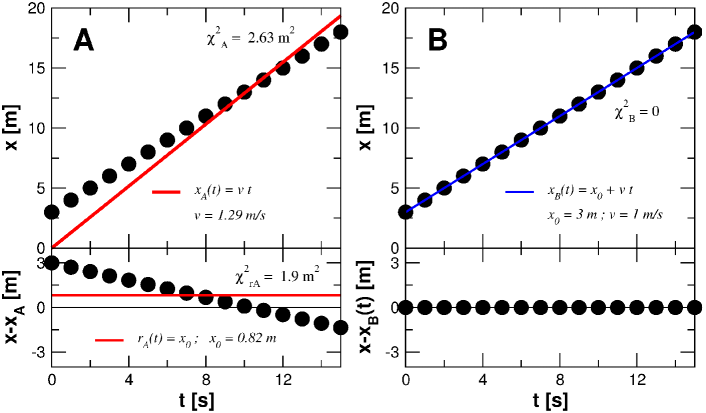
Figure 1: This example illustrates why residual statistics must not be used to assess significances in multi-parametric fits to data. We want to know whether a constant $x_{0}$ is needed to model the position $x$ of a body as a function of time $t$ (black dots). Top left panel represents the fit to the null hypothesis (model A) which only includes a velocity term (red line). Bottom left shows the residuals $r_{A}=x-x_{A}(t)$ to model A. An attempt to fit a model with a constant offset to $r_{A}$ is shown as a red line. Top right panel represents a fit adjusting all the parameters simultaneously (model B, top right panel, blue line), producing the largest possible reduction in $\chi^{2}$.

A golden rule in data-analysis is that the data should not be corrected, but it is our model which needs improvement. The inadequacy of residual analyzes can be illustrated using a trivial example (Figure 1). Let’s assume 16 measurements of the position of an object ($x$) as a function of time($t$) and no uncertainties. We are interested in its velocity but we need to decide whether constant offset $x_{0}$ is needed to model the motion. Model A (null hypothesis) consists consists in $x_{A}(t)=vt$ , where $v$ is the only free parameter, and the alternative Model B is $x_{B}(t)=x_{0}+vt$ . The question is whether including x₀ is justified given the improvement of a statistic that we define a $\chi^{2}=\frac{1}{N}\sum_{i=1}^{N}\left(x_{i}-x(t_{i})\right)^{2}$. Left panel in Figure 1 illustrates an inappropriate procedure which consist on adjusting Model A, and then deciding whether a constant $x_{0}$ is needed to explain the residuals (bottom left panel). Since such residuals are far from a constant shift, the reduction of $\chi^{2}$ is not maximal and the fit to a constant offset unsatisfactory. By subtracting model A from the data, we have created a new time-series which is no longer representative of the original one. A more meaningful procedure consists in comparing model A to a the global fit to all the parameters of model B (top right panel) achieving maximal improvement of our statistic.

Similarly, the analysis in Robertson et al.(3) only shows that the signal of GJ 581d is not present in their new residual time-series. Their procedure is summarized as follows. Their figures 1 and S3 were used to suggest RV/H_α correlations contaminating the measurements. After subtracting those correlations and the first three planets, periodograms(4-6) were applied to the residuals to show that GJ 581d fell below the detectability threshold. While the signal of GJ 581d is $K\sim 1.6$ m/s, the apparent variability induced by the RV/H_α correlations is 5 m/s peak-to-peak, and the scatter around the fits is at the $1.5-2$ m/s level. Subtracting those correlations biased the residuals by removing a model that likely included contributions from real signals and additional noise was added due to the scatter in the RV/H_α relations. All things considered, the disappearance of GJ 581d in such residual data is not surprising. Following Fig. 1, a simultaneous fit of the 30+ parameters involved would be needed to reach meaningful conclusions. Although there may be substantial RV/H_α correlations, a global optimization analysis may not support that GJ 581d is better explained by activity. A complete analysis will be presented elsewhere (see Appendix on this preprint version).

We argue that the results of Robertson et al.(3) come from the improper use of periodograms on residual data as they implement the same flawed procedure illustrated in Figure 1. Despite such periodograms are useful to provide quick-look analyses, their inadequacy to the task has been abundantly discussed in the literature(7–12). Explicitly, derived false alarm probabilities would be representative only if a model with one-sinusoid and one offset is a sufficient description of the data, measurements are uncorrelated, noise is normally distributed, and uncertainties are fully characterized (5). Every single of these hypothesis breaks down when dealing with Doppler residuals: the number of signals in not known a priori, fits to data correlate residuals, and formal uncertainties are never realistic. Proposed alternatives such as Monte Carlo bootstrapping of periodograms(5) do not help either, as those methods ignore correlations as well. Resulting biases can lead to significance assessments off by several orders of magnitude. These issues were irrelevant when Doppler amplitudes abundantly exceeded uncertainties. For example, an amplitude larger than three times the uncertainties and more than 20 measurements easily leads to false alarm probabilities smaller than 10^-6, which is much smaller than usual thresholds at 1%-0.1%. For this reason, large biases were not problematic in the early detection of gas giants (K$\sim 50$ m/s and $\sigma\sim 5$ m/s)(13), and it is the main reason why periodograms of residual data are still wide-spread tools in Doppler analyses despite their inadequacy to the task.

In summary, analysis of significance using residual data statistics leads to incorrect significance assessments. While this has been a common practice in the past, the problem is now exacerbated with signals closer to the noise and increased model complexity. The properties of the noise can be included to the model, but never subtracted from the data. This discussion directly impacts the viability of the Doppler method to find Earth-like planets. While Earth causes a 0.1 m/s wobble around the Sun, the long-term stability of the most quiet stars seems not better than 0.8 m/s(3). That is, activity induced variability can be 5-10 times larger than the signal. While global optimization does not provide absolute guarantees of success, analyzes based on residual statistics are certainly bound to failure. If activity poses an ultimate barrier to the detection of small planets, strategic long-term plans concerning large projects will need serious revision(14). It is of capital importance that analysis and verification of multi-planet claims are properly done using global-optimization techniques and by acquiring additional observations.
Acknowledgments. This work has been mostly supported by The Leverhulme Trust through grant RPG 2014-281 - PAN-Disciplinary algORithms for data Analysis. We thank H. R. A. Jones and R. P. Nelson for useful discussions and support.

References and Notes

1. M. Mayor,X. Bonfils, T. Forveille, et al. The HARPS search for southern extra-solar planets. XVIII. An Earth-mass planet in the GJ 581 planetary system. A&A 507, 487A (2009)

2. F. Pepe, C. Lovis, D. Segransan, et al. The HARPS search for Earth-like planets in the habitable zone. I. Very low-mass planets around HD 20794, HD 85512 and HD 192310. A&A 534, A58 (2011)

3. P. Robertson, S. Mahadevan, M. Endl, A. Roy. Stellar activity masquerading as planets in the habitable zone of the M dwarf Gliese 581. Science 345 (6195): 440-444 (2014)

4. N. R. Lomb. Least-squares frequency analysis of unequally spaced data, Ap&SS 39, 447L (1976)

5. A. Cummings. Detectability of extrasolar planets in radial velocity surveys, MNRAS 354, 1165C (2004)

6. M. Zechmeister, M. Kuester, The generalised Lomb-Scargle periodogram. A new formalism for the floating-mean and Keplerian periodograms A&A 496, 577Z (2009)

7. P.C. Gregory. A Bayesian Analysis of Extrasolar Planet Data for HD 73526, ApJ 631, 1198G (2005)

8. R. P. Baluev. Assessing the statistical significance of periodogram peaks, MNRAS 385, 1279B, (2008)

9. M. Tuomi. Bayesian re-analysis of the radial velocities of Gliese 581. Evidence in favour of only four planetary companions, A&A 528L, 5T (2011)

10. G. Anglada-Escude, M. Tuomi. A planetary system with gas giants and super-Earths around the nearby M dwarf GJ 676A. Optimizing data analysis techniques for the detection of multi-planetary systems, A&A 548A, 58A (2012)

11. R.D. Haywood,, A. Collier Cameron. D. Queloz, et al. Planets and stellar activity: hide and seek in the CoRoT-7 system, MNRAS 443, 2517H (2014)

12. R. Baluev. Accounting for velocity jitter in planet search surveys. MNRAS 393, 969B (2009)

13. M. Mayor, D. Queloz. A Jupiter-mass companion to a solar-type star, Nature 378, 355M (1995)

14. Several instruments aimed at precision better than 1 m/s are being proposed and/or in construction (e.g., ESPRESSO-VLT at the European Southern Observatory, TPF at the Hobby-Eberly Telescope, CARMENES at the Calar Alto Observatory, and SPIRou at the Canadian France Hawaii Telescope), because they are considered essential to detect and Earth-like planets or confirm/characterize those detected by next planet-hunting space missions (K2/NASA, TESS/NASA and PLATO/ESA).

Appendix

(pre-print version only)

Appendix A GJ 581d is not better explained by stellar activity

We present a re-analysis of the data presented in Robertson et al. (2014) (R14 hereafter) and show that the main conclusion of that manuscript (’GJ 581 does not exist’, abstract quoting) is not supported by a gobal fit to the data. The analysis is done by adding parameterized effects to the model (never subtracting them) and using the maximum likelihood statistic as a figure of merit (a generalization of the $\chi^{2}$ statistic). We limit ourselves to a frequentist framework, which is sufficient to illustrate the perils of analise based on residual statistics. In all that follows, we use exactly the same data as provided in R14 to show that the discrepant result comes from basic statistical assumptions, and it is not a matter about the quality or properties of the data.

In Section A.1, we outline the Doppler model used and show how the correlations with activity indices are introduced in it. Section A.2 reviews how to produce periodograms that account for the presence of several free parameters in addition to the new signal of interest. Results of the analysis are given in A.3. In Section A.4 we argue that, although the correlations with the I${}_{H_{\alpha}}$ index are substantial, there is no clear evidence for time-variability, and highlight the perils of applying arbitrary slicing to datasets and fitting unconstrained correlation laws. Concluding remarks are given in Section A.5.

A.1 Doppler and statistical model

Our model to predict the radial measured radial velocity $v$ of a star given the presence of k-planets is given by

$$v\left[\vec{\theta};t_{i}\right]=\gamma_{I}+\sum^{k}_{p}m[\vec{\theta}_{p},t_{i}]+\dot{v}(t_{i}-t_{0})+C_{I}\alpha_{i}$$ (1)

where $t_{i}$ is the instant of each observation, $\gamma_{I}$ is a constant offset of each instrument $I$ (or dataset), $\dot{v}$ is a term to account for a long term secular acceleration common to all datasets, and the usual Keplerian parameter of each planet candidate $p$ are consolidated in $\vec{\theta_{p}}$ : Period $P_{p}$ in days, amplitude $K_{p}$ in m s${}^{-1}~{}$, eccentricity $e_{p}$, argument of periastron $\omega_{w}$ in degrees, and initial mean $M_{0,p}$ in degrees. As discussed in R14 and already proposed in the past (eg. Queloz et al., 2001; Bonfils et al., 2007), some activity indices can linearly correlate with spurious Doppler offsets. The rightmost term accounts for such correlation and $\alpha_{i}$ is some simultaneaous activity measurement (eg. $I_{H_{\alpha}}$ provided in R14 in this case). $C_{I}$ can differ between instruments (correlations can be wavelength and resolution dependent), so one $C_{I}$ is needed for each dataset $I$. Since the mean value of the activity index is not known, a linear correlation model should also include a constant offset (eg. $v=C_{I}\alpha+b_{I}$, where $b_{I}$ should be a free parameter as well). However note that such constant is automatically absorbed by $\gamma_{I}$, further motivating the use of different $\gamma_{I}$ for each instrument. All orbital parameter values are given for a given reference epoch $t_{0}$, which we arbitrarily assume to be the first observation date.

Concerning the statistical description of the data, and under the same assumptions as R14 (white noise, statistically independent measurements), we define the logarithm of the likelihood function as

$$\ln L = -\frac{N_{\rm obs}}{2}\ln 2\pi-\frac{1}{2}\sum_{i=1}^{N_{\rm obs}}\ln\left(\epsilon_{i}^{2}+s_{I}^{2}\right)-\frac{1}{2}\sum_{i=1}^{N_{\rm obs}}\frac{\left(v_{i}-v\left[t,\vec{\theta}\right]\right)^{2}}{\epsilon_{i}^{2}+s_{I}^{2}}\,,$$ (2)

which is our merit statistic to be maximized. The $s_{I}$ parameter is often called jitter and accounts for extra white-noise of each dataset $I$. When $s_{I}=0$, maximizing this log-likelihood function is equivalent to minimizing the $\chi^{2}$ statistic. When including correlation terms to the data, the jitter parameter is even more necessary. That is, the index $\alpha$ also has uncertainties and might include variability not traced by the Doppler measurements. As for the constant offsets, $\gamma_{I}$, this extra-jitter will be accounted for through $s_{I}$ of each dataset.

R14 proposed to split the Doppler series of GJ 581 in five chunks which implicitly assume five independent sets (each one with a possibly different $\gamma_{I}$, $C_{I}$ and jitter level $s_{I}$). Details and motivation for such slicing are given in R14 and are based on apparent intervals of stronger activity and the natural yearly sampling of the data. Consequences of applying this slicing of the data are discussed later.

A.2 Likelihood-ratio periodograms

A periodogram is a representation of the improvement of some merit statistic when a sinusoidal signal is included in the model. Because of its numerical efficiency, the most widely spread algorithm to compute periodograms is the so-called Lomb-Scarge periodogram (or LS). The LS algorithm adjusts one sinusoid to each test period resulting in a plot of the period (x-axis) against the improvement of the $\chi^{2}$ statistic. A detailed derivation of the LS periodogram from $\chi^{2}$ minimization is given in Scargle (1982). Under the assumptions of the method, the peaks and significances derived from LS periodograms are only representative of a test of significance when there are no other signals present in the time-series.

This problem can be circumvented by realizing that a periodogram can be used as a representation of the overall model improvement (Baluev, 2009; Anglada-Escudé & Tuomi, 2012) by using a merit statistics of the complete model. That is, when searching for evidence of a $k+1$ periodicity, we also need to simultaneously adjust for all the other free parameters. This makes such periodograms computationally expensive, and one needs to create specific implementation of the algorithms instead of using freely distributed tools. Periodogram procedures based on adding one signal at a time are sometimes called hierarchical methods (detection is done from most significant to smaller signal). More general methods that directly explore the full parameter space exist but will not be discussed here for brevity. Some reported implementations of these include tempered Markov Chain Markov Chain algorithms (Gregory, 2011), Delayed Rejection Adaptive Metropolis (or DRAM Tuomi et al., 2014) and Markov Chains with nested sampling (Brewer & Donovan, 2015).

In our analysis, we use our custom made software to perform optimization of the likelihood function at the period search level. It differs from other Keplerian fitting codes in the sense that allows adjusting correlation coefficients, jitter parameters, and offsets as free parameters as well (further effects can be easily incorporated when necessary). For example, note that the $C_{I}$ coefficients are linear parameters, so they can be trivially incorporated in a general least-squares solver. All the parameters in $v[\vec{\theta};t_{i}]$ are converged using regular least-squares solving methods, and the parameters of the likelihood (eg. jitter terms s_I) are converged using steepest descent steps. This process is iterated a few times until a small threshold $\delta\ln L$ is registered between iterations. The solution is finally converged to the local likelihood maxima (periodogram peak) using annealing. At the signal search level, the $k+1$ signal is always considered sinusoidal (circular orbit) to avoid problems with the non-linear behaviour of high eccentricities (see discussion in Appendix A in Anglada-Escudé et al., 2013). Given that adding two more parameters($e$ and $\omega$) can only improve the fit to the data, beating a given significance threshold for the sinusoid provides a sufficient condition for detection. Significance assessments are finally provided using False alarm probability (or FAP) estimates as described in Baluev (2009, 2013b). FAPs smaller than 1% usually imply significant detections and more accurate significances can be later estimated using the integration of the Bayesian posterior distribution (eg. Tuomi & Jones, 2012). Our complete $3+1$ planet model for five datasets contains 32 free parameters: $3\times 5$ Keplerian ones, $3$ parameters for the $k+1$ sinusoid, and $3\times 5$ parameters for the five subsets. The periods of the test sinusoids are initialized over 8000 seed values uniformly sampled in frequency (1/P) between 1/1.1 and 1/20000 days^-1. The result of this procedure is illustrated in Fig. 2. Generating such periodogram took $\sim$ 30 min on a standard 2.5GHz single-core CPU. More optimal implementations of likelihood periodograms are given in Baluev (2013a).

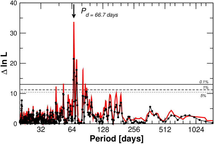
Figure 2: Likelihood ratio search for a 4th signal demonstrating that the presence of GJ 581d is still strongly supported by the data, despite the correlations with $H_{\alpha}$.

A.3 Results

The Doppler time-series and I${}_{H_{\alpha}}$ were used as provided in R14. Also as in R14, one outlying I${}_{H_{\alpha}}$ measurement was removed form the third dataset (JD = 2454610.74293 days, likely caused by a flare). R14 only removes correlations on three of the subsets based on apparently higher correlations. We allow all five coefficients to be free parameters assuming that they can be naturally zero if that value is preferred by the global fit.

As in R14, the three first signals at periods 5.3686, 12.914 and 3.1490 days (GJ 581b, GJ 581c, and GJ 581e respectively) are easily detected despite the correlations with I${}_{H_{\alpha}}$. The likelihood-ratio periodogram search for the 4-th signal (GJ 581d) is shown in Fig. 2 (red line). The signal is well detected above the 0.1% FAP line, implying a significant detection beyond reasonable doubt. The black dots represent our periodogram algorithm applied to the residuals to the 3-planet + correlations in an attempt to replicate R14 analysis more closely. While this procedure shows lower significance, we find that the significance of GJ 581d still does not fall below the 1% FAP threshold, suggesting additional relevant differences between our model and R14 (eg., jitter is not optimized in R14, and it is unclear whether constant offsets for each data chunk were solved as free parameters). In any case, the much higher value of the red curve clearly shows that significance is strongly boosted ($\Delta\ln L\sim 13$ implies $\sim e^{13}$ higher significance) when all free parameters are adjusted. This feature is characteristic of parameter degeneracy (activity signal is similar to the planet candidate’s one), but such partial degeneracy alone is not sufficient to negate the significance of a much better model on statistical grounds.

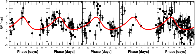
Figure 3: Doppler measurements for each subset (chronological order from left to right) after subtracting all parameterized effects (planets and correlations) except GJ 581d and phase folded to a period of 66.7 days. The red line show the maximum likelihood fit to the orbit. The signal is well traced in all the subsets (2nd,3rd and 5th) with enough observations.

A.4 No evidence for correlations changing with time

A time variable correlation can be easily explained by unrelated signals in both RV and I${}_{H_{\alpha}}$ in a similar period domain (correlation does not imply causality, see discussion in Velickovic, 2015). Just as an example, Jupiter also has an orbital period (11.86 years) comparable to the activity cycle of the Sun ($\sim$ 11 years). Unless the curves are in perfect phase, the analysis of R14 would also detect time-dependent correlations. While skepticism would be natural if only one cycle was covered, accumulated observations over several cycles would clearly differentiate both signals (unless one keeps adjusting a time-dependent correlation on arbitrary data-slices). The Sun-Jupiter example can be compared to the period of 66.7 days of GJ 581d to the signal in I${}_{H_{\alpha}}$ at $\sim$ 130 days (and harmonics) discussed in R14. A second consequence of forcing corrections into the Doppler time-series is the increase in the noise floor for the RVs themselves. That is, Doppler time-series become limited by the scatter in the activity indices, and -what is worse- they can be severely contaminated by correlated variability of the indices as well.

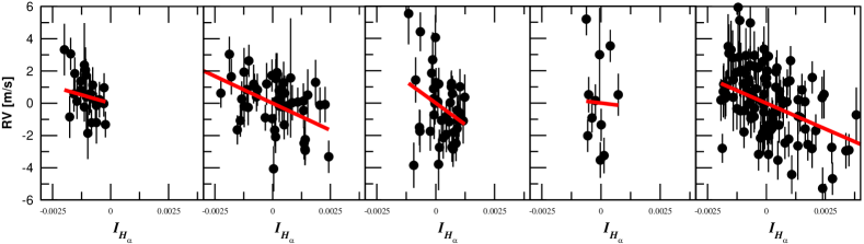
Figure 4: Doppler versus H_α correlation plots for each subset. As for the phased plots in Figure 3, all signals except the H${}_{a}lpha$/RV correlation have been subtracted to improve visualization. The correlation slopes of the sets with more observations (2nd and 5th panel) cast serious doubt on the proposed time-variability of the correlation law. The values of the measured slopes are $C_{1}=-420$ m s${}^{-1}~{}$, $C_{2}=-670$ m s${}^{-1}~{}$, $C_{3}=-1040$ m s${}^{-1}~{}$, $C_{4}=-190$ m s${}^{-1}~{}$and $C_{5}=-630$ m s${}^{-1}~{}$, being $C_{1}$ and and $C_{4}$ the smallest but also most uncertain given the small ammount of observations in those subsets.

While we agree with R14 that correlations of RV/I${}_{H_{\alpha}}$ are significant, our analysis does not support the reported time-dependence of the correlation either. Note that more discrepant slopes in Figure 4 (Panels 1 and 4) correspond to seasons where the number of points and the range of H_α variability is much smaller. Given that the model is very complex (30+ parameters) and non-linear, proper quantification of the uncertainties in the correlation coefficients requires sampling techniques of the posterior density (eg. Monte Carlo Markov Chain sampling of the posterior) which is beyond our scope here.

A.5 Conclusions

The failure to confirm GJ 581d by R14 seems to be related to the analysis of residual data and improper interpretation of periodograms. R14 attempted several correlations with activity indices and applied a rather arbitrary slicing of the datasets. Furthermore, selecting apparently active sub-sets and fitting correlations to those should be avoided as it constitutes a circular argument. The same problem likely explains the non-detection of the very significant signal GJ 667Cd in Robertson & Mahadevan (2014), even under the assumption of white noise. In that case, the authors sliced the RV time-series and forced correlations with another activity index (the so-called FWHM). As for GJ 581d -and Jupiter for the Sun-, GJ 667C also show evidence for variability in periods comparable ($P_{\rm FWHM}\sim 105$ days) to the period of the proposed planet candidate ($P_{d}=91$ days). Again, removing time-dependent correlations on data slices necessarily decrease their apparent significance, especially in periodograms of residual data.

The validity of the various models and methods to account for noise in Doppler data is a hotly debated topic. Contributions to the discussion on benchmark systems should ensure that the applied statistical tools are formally correct. Given all these caveats, the analysis presented in R14 should be considered inconclusive, and GJ 581d should be reinstated as a planet candidate until additional observations suggest otherwise.

References

- Anglada-Escudé & Tuomi (2012) Anglada-Escudé G., Tuomi M., 2012, A&A, 548, A58
- Anglada-Escudé et al. (2013) Anglada-Escudé G., Tuomi M., Gerlach E., Barnes R., Heller R., Jenkins J. S., Wende S., Vogt S. S., Butler R. P., Reiners A., Jones H. R. A., 2013, A&A, 556, A126
- Baluev (2009) Baluev R. V., 2009, MNRAS, 393, 969
- Baluev (2013a) Baluev R. V., 2013a, Astronomy and Computing, 2, 18
- Baluev (2013b) Baluev R. V., 2013b, MNRAS, 429, 2052
- Bonfils et al. (2007) Bonfils X., Mayor M., Delfosse X., Forveille T., Gillon M., Perrier C., Udry S., Bouchy F., Lovis C., Pepe F., Queloz D., Santos N. C., Bertaux J.-L., 2007, A&A, 474, 293
- Brewer & Donovan (2015) Brewer B. J., Donovan C. P., 2015, arXiv:1501.06952 (MNRAS accepted)
- Cumming (2004) Cumming A., 2004, MNRAS, 354, 1165
- Gregory (2005) Gregory P. C., 2005, ApJ, 631, 1198
- Gregory (2011) Gregory P. C., 2011, MNRAS, 410, 94
- Queloz et al. (2001) Queloz D., Henry G. W., Sivan J. P., Baliunas S. L., Beuzit J. L., Donahue R. A., Mayor M., Naef D., Perrier C., Udry S., 2001, A&A, 379, 279
- Robertson & Mahadevan (2014) Robertson P., Mahadevan S., 2014, ApJ, 793, L24
- Robertson et al. (2014) Robertson P., Mahadevan S., Endl M., Roy A., 2014, Science, 345, 440
- Scargle (1982) Scargle J. D., 1982, ApJ, 263, 835
- Tuomi et al. (2014) Tuomi M., Anglada-Escude G., Jenkins J. S., Jones H. R. A., 2014, arXiv:1405.2016 (submitted to MNRAS)
- Tuomi & Jones (2012) Tuomi M., Jones H. R. A., 2012, A&A, 544, A116
- Velickovic (2015) Velickovic V., 2015, American Scientist, 103, 26