Abstract

Using a holographic method, we further investigate the relaxation towards the hydrodynamic regime of a boost-invariant non-Abelian plasma taken out-of-equilibrium. In the dual description, the system is driven out-of-equilibrium by boundary sourcing, a deformation of the boundary metric, as proposed by Chesler and Yaffe. The effects of several deformation profiles on the bulk geometry are investigated by the analysis of the corresponding solutions of the Einstein equations. The time of restoration of the hydrodynamic regime is investigated: setting the effective temperature of the system at the end of the boundary quenching to $T_{eff}(\tau^{*})=500$ MeV, the hydrodynamic regime is reached after a lapse of time of ${\cal O}$(1 fm/c).

PACS numbers: 12.38.Mb, 11.25.Tq
Keywords: Gauge-gravity correspondence, Holography and quark-gluon plasma

1 Introduction

The possibility of employing the gauge/gravity duality correspondence [1, 2, 3] to the analysis of far-from-equilibrium processes in strongly coupled systems has enlarged the realm of nonperturbative phenomena to which this theoretical method can be applied in a quite controllable way, while traditional approaches are less effective. Among the different systems, of particular interest is the one produced in ultrarelativistic heavy ion collisions (HI), as those taking place at RHIC and at LHC. The features of this system, for time scales larger than about 1 fm/c, seem to be well reproduced in a hydrodynamic setup involving a strongly coupled/low viscosity fluid [5, 6], a framework allowing to correctly describe experimental observables such as the light hadron transverse momentum spectra. In the hydrodynamic scheme of crucial importance are, after the pre-equilibrium regime following the collisions, the conditions at the time when the hydrodynamic behavior sets up. In particular, at this time the system stress-energy tensor $T^{\mu}_{\nu}$ is important. We write it as

$$T^{\mu}_{\nu}=\frac{N_{c}^{2}}{2\pi^{2}}\,diag(-\epsilon,p_{\perp},p_{\perp},p_{\parallel})\,\,\,,$$ (1)

in terms of the system energy density $\epsilon$ and of $p_{\perp},p_{\parallel}$ the pressures along one of the two transverse directions (with respect to the collision axis) and in the longitudinal direction, respectively . For example, in approaches based on the idea of an initial state described by color glass condensate with a saturation scale $Q_{s}$ of the order of a few GeV, the initial stress-energy tensor comes from classical chromo-electric and chromo-magnetic fields and has the form $T^{\mu}_{\nu}\propto diag(-\epsilon,\epsilon,\epsilon,-\epsilon)$. However, such an initial condition has been shown to be unstable, as soon as one-loop corrections in the strong coupling constant are switched on [7].

In the analysis presented in our study, a prominent role is therefore played by the stress-energy tensor, which is needed to understand the features of the equilibrium regime, the time needed to reach equilibrium, and the properties of the dynamics driving the system towards equilibrium. Questions to be answered are, for a system driven out-of-the-equilibrium, whether the late-time state is described by hydrodynamics, and whether the elapsed time needed to reach equilibrium is related to the dynamics during the out-of-equilibrium state. These issues concerning the transient process from a far-from-equilibrium to a hydrodynamic regime can be faced in the holographic approach [8], using as a guideline the conjectured correspondence between a supersymmetric, conformal field theory defined in a four dimensional (4D) space-time and a gravity theory in a higher dimensional space-time, a five dimensional Anti de-Sitter space (AdS₅) times a five dimensional sphere S⁵ [1]. The gauge theory is defined on the 4D boundary of AdS₅, and the connection has been extended to the case of nonlinear fluid dynamics [9]. Non-equilibrium can be studied by solving in the bulk the 5D Einstein equations for the metric subject to suitable time-dependent boundary conditions. Information about the late-time regime can be obtained computing various invariants. For example, in Ref.[10] the square of the Riemann tensor $\Re^{2}$ (the Kretschmann scalar) has been studied as an expansion in inverse powers of the proper time up to second order, finding that, in the asymptotic $\tau\to\infty$ regime, the scalar $\Re^{2}$ is free of singularities in the perfect fluid case. The boundary theory stress-energy tensor results from the solutions of the Einstein equations in the bulk.

Analyses in the case of boost-invariant fluid [11, 12], for some choices of the profile distortion, have shown the formation of a horizon in the bulk, and have given access to the components of the boundary theory stress-energy tensor. The investigations have been extended to samples of initial states characterized by different values of the components of the stress-energy tensor, without reference to the mechanism producing each state [13, 14, 15, 16, 17, 18].

As formulated in [11, 12], the initial off-equilibrium states can be thought as being produced by external sources distorting the boundary metric for short time intervals. We focus on this issue, with a study of external distortion profiles, step-shaped or short-duration sequences repeating themselves with different intensities, with the aim of describing phenomena where a small number of collisions takes place before the system starts evolving to thermal equilibrium. This study in the boost-invariant framework is useful for more involved cases where a lower symmetry is assumed for the system, for example in shock-wave collisions [19, 20, 21, 22].

There are several reasons to study complex distortion shapes in the boundary metric. The bulk Einstein equations are nonlinear, and different distorsions produce unrelated responses. The resulting effective temperature and entropy density follow different profiles as a consequence of the boundary sourcing. Moreover, it is interesting to investigate whether the onset of the hydrodynamic regime is related to the distortion curve. Finally, these analyses have to face problems concerning the stability of the solution of GR equations with different boundary conditions.

The plan of the present paper, in which a few of the above issues are examined, is the following. In Section 2 we describe how a system is taken out-of-equilibrium through the distortion of the boundary metric, as done in [11, 12]. We discuss a suitable procedure for solving the resulting 5D Einstein equations, providing a few details of the algorithm and the issue of the stability of the solutions. In Section 3 we describe the profiles of the boundary geometry distortion we have chosen to study, with the motivations. In Section 4 we discuss our findings, in particular concerning the equilibration time. The conclusions are presented in the last Section. Details dealing with the calculation of the boundary stress-energy tensor $T^{\mu}_{\nu}$ are collected in appendix A, while in appendix B we discuss some aspects of the numerical algorithm.

2 Distorting the boundary

The main idea, as in [11, 12], is to study the effects of a time-dependent deformation of the metric of the 4D boundary. As a consequence of the deformation, gravitational radiation is produced and propagates in the 5D bulk, and a black hole is formed together with its horizon. In this way, one can trade the study of the reach of equilibrium in the 4D boundary theory for the analysis of the time evolution of the geometry in the 5D bulk.

We set the 4D coordinates $x^{\mu}=(x^{0},x^{1},x^{2},x^{3})$, identifying $x^{3}=x_{\parallel}$ with the axis in the direction of collisions and along which the plasma expands. Boost-invariance along that axis is imposed, together with translation invariance and $O(2)$ rotation invariance in the orthogonal plane $x_{\perp}=\{x^{1},\,x^{2}\}$. In terms of the proper time $\tau$ and rapidity $y$, given by $x^{0}=\tau\cosh y$, $x_{\parallel}=\tau\sinh y$, the 4D Minkowski line element is given by $ds^{2}=-d\tau^{2}+dx_{\perp}^{2}+\tau^{2}dy^{2}$.

A distortion of the boundary metric, leaving the spatial three-volume unchanged and respecting the imposed symmetries, can be obtained through a function $\gamma(\tau)$ which encodes information about a deformation:

$$ds^{2}=-d\tau^{2}+e^{\gamma(\tau)}dx_{\perp}^{2}+\tau^{2}e^{-2\gamma(\tau)}dy^{2}\,\,.$$ (2)

The space-time with the metric (2) is considered as the boundary of the 5D space-time in which the gravity dual is defined. We adopt 5D Eddington-Finkelstein coordinates, with $r$ the extra-dimension coordinate and the boundary reached for $r\to\infty$. In general, the 5D bulk metric can be chosen as

$$ds^{2}=2drd\tau-Ad\tau^{2}+\Sigma^{2}e^{B}dx_{\perp}^{2}+\Sigma^{2}e^{-2B}dy^{2}\,\,\,,$$ (3)

with the functions $A$, $\Sigma$ and $B$ only depending on $r$ and $\tau$ to respect the adopted symmetries. The behavior of these functions against the deformation allows us to describe how the bulk metric changes as a consequence of the distortion of the boundary. With the metric (3), at fixed $x_{\perp}$ and rapidity $y$, infalling radial null geodesics correspond to constant $\tau$, while outgoing radial null geodesics are obtained from $\displaystyle\frac{dr}{d\tau}=\frac{A(r,\tau)}{2}$. Therefore, for a generic function $\xi(r,\tau)$ the derivatives

$$\xi^{\prime} = \partial_{r}\xi$$ (4)

$${\dot{\xi}} = \partial_{\tau}\xi+\frac{1}{2}A\partial_{r}\xi$$ (5)

represent directional derivatives along the infalling radial null geodesics and the outgoing radial null geodesics, respectively.

The 5D metric (3) is the solution of Einstein’s equations with negative cosmological constant. In terms of $A(r,\tau)$, $\Sigma(r,\tau)$ and $B(r,\tau)$ the equations can be rephrased as [12]:

$$\Sigma({\dot{\Sigma}})^{\prime}+2\Sigma^{\prime}{\dot{\Sigma}}-2\Sigma^{2}=0$$ (6)

$$\Sigma({\dot{B}})^{\prime}+\frac{3}{2}\left(\Sigma^{\prime}{\dot{B}}+B^{\prime}{\dot{\Sigma}}\right)=0$$ (7)

$$A^{\prime\prime}+3B^{\prime}{\dot{B}}-12\frac{\Sigma^{\prime}{\dot{\Sigma}}}{\Sigma^{2}}+4=0$$ (8)

$${\ddot{\Sigma}}+\frac{1}{2}\left({\dot{B}}^{2}\Sigma-A^{\prime}{\dot{\Sigma}}\right)=0$$ (9)

$$\Sigma^{\prime\prime}+\frac{1}{2}B^{\prime 2}\Sigma=0\,\,.$$ (10)

The five equations (6)-(10) can be considered as three dynamical and two constraint equations. The condition that the metric (3) produces the 4D metric (2) at the boundary, for $r\to\infty$, constrains the large $r$ behavior of $A(r,\tau)$, $\Sigma(r,\tau)$ and $B(r,\tau)$:

$$\frac{A(r,\tau)-r^{2}}{r}\xrightarrow[r\to\infty]{}0\,\,,$$ (11)

$$\frac{\Sigma(r,\tau)}{r}\xrightarrow[r\to\infty]{}\tau^{\frac{1}{3}}\,\,,$$ (12)

$$B(r,\tau)\xrightarrow[r\to\infty]{}-\frac{2}{3}\log\tau+\gamma(\tau)\,\,.$$ (13)

The invariance of (3) under the diffeomorphism $r\to r+\lambda(\tau)$ has been exploited to impose the large $r$ condition for $A$.

We switch on the distortion of the boundary metric at the initial time $\tau=\tau_{i}$, starting from the AdS₅ bulk metric:

$$ds^{2}=2drd\tau+r^{2}\left[-d\tau^{2}+dx_{\perp}^{2}+\left(\tau+\frac{1}{r}\right)^{2}dy^{2}\right]\,\,\,.$$ (14)

As discussed in [14], taking the limit $r\to\infty$ and $\tau\to 0$ with the Eddington-Finkelstein coordinates, Eq. (14), is ambiguous. For this reason, we set $\tau_{i}>0$. The initial conditions for $A$, $\Sigma$ and $B$ are therefore:

$$A(r,\tau_{i}) = A_{ini}(r)=r^{2}\,\,\,,$$ (15)

$$\Sigma(r,\tau_{i}) = \Sigma_{ini}(r)=r\left(\tau_{i}+\frac{1}{r}\right)^{1/3}\,\,\,,$$ (16)

$$B(r,\tau_{i}) = B_{ini}(r)=-\frac{2}{3}\log\left(\tau_{i}+\frac{1}{r}\right)\,\,\,.$$ (17)

For $r\to\infty$, the Einstein’s equations can be solved starting from the relations (11)-(13). As suggested in [11, 12], for $A(r,\tau)$, $\Sigma(r,\tau)$ and $B(r,\tau)$ the large-$r$ expansions can be written as

$$A_{asy}(r,\tau) = \sum_{n=0}\left[a_{n}(\tau)+\alpha_{n}(\tau)\log r\right]r^{2-n}\,\,,$$ (18)

$$\Sigma_{asy}(r,\tau) = \sum_{n=0}\left[s_{n}(\tau)+\sigma_{n}(\tau)\log r\right]r^{1-n}\,\,,$$ (19)

$$B_{asy}(r,\tau) = \sum_{n=0}\left[b_{n}(\tau)+\beta_{n}(\tau)\log r\right]r^{-n}\,\,\,.$$ (20)

The conditions (11)-(13) fix the $n=0$ coefficients in (18)-(20), as well as those for $n=1$ in $A_{asy}$. The other coefficients can be determined imposing that Eqs. (6)-(8) are satisfied by the functions (18)-(20), but this leaves two coefficients undetermined, $a_{4}(\tau)$ and $b_{4}(\tau)$. From Eq. (10) a relation follows between $a_{4}$ and $b_{4}$:

$$b_{4}(\tau)=\frac{1296\tau^{5}a_{4}^{\prime}(\tau)+1728\tau^{4}a_{4}(\tau)+G(\tau)}{1728\tau^{4}\left(-2+3\tau\gamma^{\prime}(\tau)\right)}\,\,,$$ (21)

with the primes denoting derivatives with respect to $\tau$, and the function $G(\tau)$ expressed in terms of $\gamma^{(n)}(\tau)=\frac{d^{n}\gamma(\tau)}{d\tau^{n}}$:

$$G(\tau) = -576+3618\tau\gamma^{\prime}(\tau)-\tau^{2}\left(6903\gamma^{\prime}(\tau)^{2}+1474\gamma^{\prime\prime}(\tau)\right)$$ (22)

$$+ \tau^{3}\left(4608\gamma^{\prime}(\tau)^{3}+5199\gamma^{\prime}(\tau)\gamma^{\prime\prime}(\tau)+468\gamma^{(3)}(\tau)\right)$$

$$+ \tau^{4}\left(-918\gamma^{\prime}(\tau)^{4}-6480\gamma^{\prime}(\tau)^{2}\gamma^{\prime\prime}(\tau)+216\gamma^{\prime\prime}(\tau)^{2}-540\gamma^{\prime}(\tau)\gamma^{(3)}(\tau)+306\gamma^{(4)}(\tau)\right)$$

$$+ \tau^{5}\left(3240\gamma^{\prime}(\tau)^{3}\gamma^{\prime\prime}(\tau)+162\gamma^{\prime\prime}(\tau)\gamma^{(3)}(\tau)-459\gamma^{\prime}(\tau)\gamma^{(4)}(\tau)\right)\,\,.$$

In our procedure, $a_{4}(\tau)$ and $b_{4}(\tau)$ are determined by Eq. (21) and matching the computed functions $\Sigma$ and $B$ with their asymptotic expressions (19) and (20) for large $r$. Using $a_{4}(\tau)$ and $b_{4}(\tau)$, important observables can be obtained, such as the components of the boundary stress-energy tensor $T^{\mu}_{\nu}$, as discussed in next sections.

The details of our method for solving Eqs. (6)-(10) are as follows. In the set of functions $\Sigma$, $\dot{\Sigma}$, $B$, $\dot{B}$ and $A$, we treat a given function and its derivative (5) as independent. At $\tau=\tau_{i}$, $\Sigma(r,\tau_{i})$, $B(r,\tau_{i})$ and $A(r,\tau_{i})$ are known, Eqs. (15)-(17). To complete the set of initial conditions, we compute $\dot{\Sigma}(r,\tau_{i})$ and $\dot{B}(r,\tau_{i})$ solving Eqs. (6) and (7), respectively.

At $\tau>\tau_{i}$ the algorithm is organized in steps.

1. Using the definition (5), we determine $\partial_{\tau}\Sigma(r,\tau_{i})$ and $\partial_{\tau}B(r,\tau_{i})$, which allow us to obtain $\Sigma$ and $B$ at the subsequent time $\tau_{i}+d\tau$, if $d\tau$ is small enough for the equations

   $$\Sigma(r,\tau_{i}+d\tau)=\Sigma(r,\tau_{i})+d\tau\partial_{\tau}\Sigma(r,\tau_{i})$$

   $$B(r,\tau_{i}+d\tau)=B(r,\tau_{i})+d\tau\partial_{\tau}B(r,\tau_{i})$$

   to be valid.

2. Once $\Sigma(r,\tau_{i}+d\tau)$ and $B(r,\tau_{i}+d\tau)$ are determined, we compute $a_{4}(\tau_{i}+d\tau)$ and $b_{4}(\tau_{i}+d\tau)$. Indeed, $a_{4}(\tau_{i}+d\tau)$ can be obtained fitting the computed functions $\Sigma(r,\tau_{i}+d\tau)$ and $B(r,\tau_{i}+d\tau)$ with their asymptotic expressions (19) and (20) in the range $r_{as}\leqslant r\leqslant r_{max}$ (later on in this section, it will be shown how to set $r_{as})$. Then, we get $b_{4}(\tau_{i}+d\tau)$ from Eq. (21).

3. $\dot{\Sigma}(r,\tau_{i}+d\tau)$, $\dot{B}(r,\tau_{i}+d\tau)$ and finally $A(r,\tau_{i}+d\tau)$ are computed solving Eqs. (6)-(8); the boundary conditions are fixed using (19), (20), (18), and $a_{4}(\tau_{i}+d\tau)$ and $b_{4}(\tau_{i}+d\tau)$.

With the functions known at $\tau_{i}+d\tau$, the cycle is repeated until a chosen final value of $\tau$ is reached. Typically, with the $\gamma$ functions considered in our analysis we use $d\tau=10^{-2}$.

At each $\tau$ step, our solution algorithm requires three values of the bulk coordinate $r$: $r_{max}$ and $r_{min}$, which are the maximum and minimum value of $r$ used in the numerical calculation, and $r_{as}$, a value employed to determine $a_{4}(\tau)$ from the asymptotic expressions (18)-(20) used in the range $[r_{as},r_{max}]$. Stability against variation of such parameters is used as a criterium to check the numerical results. Particularly relevant is the minimum value $r_{min}$, required to perform an excision in the bulk coordinates. This value is set in the following way. At fixed $\tau$, for each one of Eqs. (6)-(10) we construct the function ${\cal R}_{i}(r,\tau)$ defined as the absolute value of the l.h.s. of the equation divided by the sum of the absolute value of its addendi (see appendix B for definitions). At $\tau=\tau_{i}$, we choose a small initial value of $r_{min}$; then, at each $\tau$, $r_{min}$ is increased by steps of size typically $0.005$, until the differential equations (6)-(8) and one constraint equation (10) are fulfilled, namely by requiring the condition ${\cal R}_{i}(r_{min},\tau)<0.03$ for $i=6,7,8,10$. As a result, the bulk excision is always beyond the apparent horizon. In $r_{min}$, the function $A(r_{min},\tau)$ becomes negative but not large, hence possible singularities beyond the horizon are avoided. A similar procedure is carried out for $r_{as}$. We initially set $r_{as}$, and then we gradually increase it until the condition ${\cal R}_{i}(r_{as},\tau)<0.01$ for $i=6,7,8,10$ is satisfied. Therefore, at this stage, we monitor the accuracy of the three differential equations and one constraint equation in $r_{min}$ and $r_{as}$. At the end of the procedure, we check that the condition ${\cal R}_{i}\leq 0.01$ is fulfilled for all Eqs. (6)-(10), i.e. $i=6-10$, and in the whole $(r,\tau)$ range. We find that this is indeed the case except for few tiny regions. In the largest part of the $(r,\,\tau)$ plane deviations from zero are smaller than ${\cal O}(10^{-4})$, as discussed in appendix B. During the numerical evaluation, no corrections are required to account for the finite value of the time step. In spite of the intricacy of the boundary conditions, stable solutions are found.

3 Models for the distortion of the boundary geometry

We are interested in investigating deformations of the boundary metric characterized by different duration, intensity and structure. We set the generic form for $\gamma(\tau)$:

$$\gamma(\tau)=w\left[Tanh\left(\frac{\tau-\tau_{0}}{\eta}\right)\right]^{7}\,+\sum_{j=1}^{N}\gamma_{j}(\tau,\tau_{0,j})$$ (23)

with

$$\gamma_{j}(\tau,\tau_{0,j})=c_{j}f_{j}(\tau,\tau_{0,j})^{6}e^{-1/f_{j}(\tau,\tau_{0,j})}\Theta\left(1-\frac{(\tau-\tau_{0,j})^{2}}{\Delta_{j}^{2}}\right)\,\,$$ (24)

and

$$f_{j}(\tau,\tau_{0,j})=1-\frac{(\tau-\tau_{0,j})^{2}}{\Delta_{j}^{2}}\,\,\,.$$ (25)

This expression generalizes the one used in [12], and represents sequences of $N$ ”pulses”, each one of intensity $c_{j}$ and duration proportional to $\Delta_{j}$, with the possibility of superimposing a smooth deformation, of intensity $w$, which asymptotically changes the scales of the coordinates. After their generation, pulses travel in the longitudinal direction $x_{\parallel}$, driving the boundary state out-of-equilibrium. The response of the $5D$ bulk geometry to this deformation describes how equilibrium is reached at late times. We choose three different models, $\cal A$, $\cal B$ and $\cal C$, setting the various parameters in Eqs. (23)-(25).

Model $\cal A$ represents two pulses in the boundary metric. The parameters are set to $w=0$ and $N=2$, $c_{1}=1$, $\Delta_{1,2}=1$, $\tau_{0,1}=\frac{5}{4}\Delta_{1}$, $c_{2}=2$. Moreover, two different values of $\tau_{0,2}$: $\tau_{0,2}=\frac{17}{4}\Delta_{2}$ and $\tau_{0,2}=\frac{9}{4}\Delta_{2}$ are considered, changing the time interval between the pulses. The final time of the distortion is $\tau_{f}^{\cal A}=5.25$ and $\tau_{f}^{\cal A}=3.25$ for the two cases, respectively, two quantities important for our discussion.

In model $\cal B$ we set $w=\frac{2}{5}$, $\eta=1.2$, $\tau_{0}=0.25$, $N=1$, $c_{1}=1$, $\Delta_{1}=1$, $\tau_{0,1}=4\Delta_{1}$, and the short pulse ends at $\tau_{f}^{\cal B}=5$ while a tale of the distortion continues with $\tau$ and approaches a constant value.

Model $\cal C$ combines both the previous ones, and is obtained using

$$w = \frac{2}{5},\,\,\,\,\,\eta=1.2,\,\,\,\,\,\tau_{0}=0.25\,\,,$$

$$c_{0,1} = 0.5,\,\,\,\,\,c_{0,2}=1,\,\,\,\,\,c_{0,3}=0.35,\,\,\,\,\,c_{0,4}=0.3,$$

$$\tau_{0,1} = \tau_{0}+1.5,\,\,\,\,\,\tau_{0,2}=\tau_{0}+3.8,\,\,\,\,\,\tau_{0,3}=\tau_{0}+6.1,\,\,\,\,\,\tau_{0,4}=\tau_{0}+8.4,$$

$$\Delta_{j} = 0.8\,\,\,\,\,(j=1,2,3,4)\,\,.$$

For this model the last short pulse ends at $\tau_{f}^{\cal C}=9.45$. As mentioned, to avoid in the Eddington-Finkelstein coordinates the ambiguity in the limits $r\to\infty$ and $\tau\to 0$, in all cases the initial time is $\tau_{i}>0$. The three profiles $\gamma(\tau)$ are depicted in Figs. 2, 5 and 8.

The distortion profiles are chosen with the purpose of studying different situations. Model $\cal A$ is the repetition, in the boundary metric, of two short pulses of different intensity, Fig. 2. In particular, we consider two cases with different interval of time between the pulses, ranging from the condition of distant perturbations to the case of overlapping pulses. This model can provide us with information on the horizon formation, in comparison with the case of isolated pulse studied in [12], and on the effects related to the time elapsed between the distortions. Model $\cal B$ has the purpose of studying a combination of two effects with very different time scales, a short pulse and a slow continuum asymptotically producing a rescaling of the boundary coordinates. Model $\cal C$, a combination of the previous cases, accounts for the effects of several pulses with various intensities, and is closer to physical processes driving systems out-of equilibrium in relativistic heavy ion collisions. In all cases, the horizon formation and behavior are investigated, together with the various components the boundary stress-energy tensor, looking at the time when the hydrodynamic regime sets in.

4 Results and discussions

In the numerical calculation for the models previously described, the solutions of the bulk Einstein equations allow to obtain the apparent horizon and the event horizon, which define the system temperature $T_{eff}$. The apparent horizon is determined as the locus of points where the condition $\dot{\Sigma}(r_{h},\tau)=0$ is fulfilled. The event horizon, which separates causally disconnected regions, is found drawing outgoing radial null geodesic curves and looking for the critical curve which separates the geodesics escaping towards the boundary from the ones plunging back in the bulk. From these curves, the function $r_{h}(\tau)$ ($r_{h}(\tau)$ being the position of the horizon at the proper time $\tau$) is determined, which defines the temperature $T_{eff}(\tau)$. Asymptotically in proper time, the apparent horizon and the event horizon coincide. From the solution, $\Sigma(r_{h},\tau)^{3}$, the area of each horizon per unit of rapidity, can be computed.

The three models share common features, which we discuss together with the differences. Before presenting this analysis, let us recall a few results concerning the boundary stress-energy tensor $T^{\mu}_{\nu}$.

As discussed in the Bjorken’s seminal paper [27], under the assumptions of homogeneity, boost-invariance and invariance under rotations in the transverse plane with respect to the fluid velocity, the fluid stress-energy tensor $T_{\mu}^{\nu}$ has well-defined properties, and its components only depend on the proper time $\tau$, a manifestly boost-invariant condition. Imposing $T_{\mu}^{\nu}$ conservation and traceless conditions, the tensor components can be expressed in terms of a single function $f(\tau)$, that can be chosen to be $-T_{0}^{0}$:

$$T_{\mu}^{\nu}=diag\left(-f(\tau),\,f(\tau)+\displaystyle{\frac{1}{2}}\tau f^{\prime}(\tau),\,f(\tau)+\displaystyle{\frac{1}{2}}\tau f^{\prime}(\tau),\,-f(\tau)-\tau f^{\prime}(\tau)\right)\,\,\,\ .$$ (26)

For a perfect fluid, the equation of state $\epsilon=3p$, with $p=p_{\parallel}=p_{\perp}$, fixes the $\tau$ dependence: $\epsilon(\tau)=\displaystyle{\frac{const}{\tau^{4/3}}}$, stemming from the relations

$$p_{\parallel}(\tau) = -\epsilon(\tau)-\tau\epsilon^{\prime}(\tau)$$ (27)

$$p_{\perp}(\tau) = \epsilon(\tau)+\frac{\tau}{2}\epsilon^{\prime}(\tau)\,\,\,.$$ (28)

Deviations from the ideal behavior can be included as corrections taking viscous effects into account, in a gradient expansion. On the gauge theory side, the gradient expansion corresponds to a late time expansion, with subleading terms identified with the dissipative ones in the hydrodynamical theory. As shown in [10], the function $f(\tau)$ deviates from $f(\tau)=const/\tau^{4/3}$ if the assumption of perfect fluid behavior is removed. For example, the case $\epsilon(\tau)\sim\displaystyle{\frac{1}{\tau^{s}}}$ corresponds to $p_{\parallel}\sim\displaystyle{\frac{(s-1)}{\tau^{s}}}$ and $p_{\perp}\sim\displaystyle{\frac{(2-s)}{2\tau^{s}}}$.  Subleading corrections to the perfect fluid behavior relate the energy density

$$\epsilon(\tau)=\frac{3}{4}\pi^{4}T_{eff}(\tau)^{4}$$ (29)

to the definition of an effective temperature $T_{eff}(\tau)$. The calculation in ${\cal N}=4$ SYM gives [28, 29, 14]:

$$T_{eff}(\tau) = \frac{\Lambda}{(\Lambda\tau)^{1/3}}\Bigg{[}1-\frac{1}{6\pi(\Lambda\tau)^{2/3}}+\frac{-1+\log 2}{36\pi^{2}(\Lambda\tau)^{4/3}}$$ (30)

$$+ \frac{-21+2\pi^{2}+51\log 2-24(\log 2)^{2}}{1944\pi^{3}(\Lambda\tau)^{2}}+{\cal O}\left(\frac{1}{(\Lambda\tau)^{8/3}}\right)\Bigg{]}\,\,\ .$$

This leads to

$$\epsilon(\tau) = \frac{3\pi^{4}\Lambda^{4}}{4(\Lambda\tau)^{4/3}}\left[1-\frac{2c_{1}}{(\Lambda\tau)^{2/3}}+\frac{c_{2}}{(\Lambda\tau)^{4/3}}+{\cal O}\left(\frac{1}{(\Lambda\tau)^{2}}\right)\right]$$ (31)

$$p_{\parallel}(\tau) = \frac{\pi^{4}\Lambda^{4}}{4(\Lambda\tau)^{4/3}}\left[1-\frac{6c_{1}}{(\Lambda\tau)^{2/3}}+\frac{5c_{2}}{(\Lambda\tau)^{4/3}}+{\cal O}\left(\frac{1}{(\Lambda\tau)^{2}}\right)\right]$$ (32)

$$p_{\perp}(\tau) = \frac{\pi^{4}\Lambda^{4}}{4(\Lambda\tau)^{4/3}}\left[1-\frac{c_{2}}{(\Lambda\tau)^{4/3}}+{\cal O}\left(\frac{1}{(\Lambda\tau)^{2}}\right)\right]\,\,\,,$$ (33)

and to the pressure ratio and anisotropy:

$$\frac{p_{\parallel}}{p_{\perp}} = 1-\frac{6c_{1}}{(\Lambda\tau)^{2/3}}+\frac{6c_{2}}{(\Lambda\tau)^{4/3}}+{\cal O}\left(\frac{1}{(\Lambda\tau)^{2}}\right),$$ (34)

$$\frac{\Delta p}{\epsilon} = \frac{p_{\perp}-p_{\parallel}}{\epsilon}=2\left[\frac{c_{1}}{(\Lambda\tau)^{2/3}}+\frac{2c_{1}^{2}-c_{2}}{(\Lambda\tau)^{4/3}}+{\cal O}\left(\frac{1}{(\Lambda\tau)^{2}}\right)\right]\,\,\,,$$ (35)

with $c_{1}=\displaystyle{\frac{1}{3\pi}}$ and $c_{2}=\displaystyle{\frac{1+2\log{2}}{18\pi^{2}}}$. $\Lambda$ is a parameter to be determined for each one of the considered models.

Understanding the results of the calculation of the solutions of the 5D Einstein equations, hence, requires the computation of the boundary stress-energy tensor $T^{\mu}_{\nu}$ in Eq. (1) and the comparison with the proper time dependence following the previous equations. The various components of the stress-energy tensor of the boundary theory can be determined using the holographic renormalization procedure developed in [30, 31] and shortly described in appendix A. The functions $a_{4}(\tau)$ and $b_{4}(\tau)$ in the expansions (18) and (20), computed through the Einstein equations, are required, and the energy density and the longitudinal and parallel pressures are obtained in terms of such functions:

$$\epsilon = -\frac{3}{4}a_{4}+\tilde{\epsilon}_{\gamma}\,\,\,,$$ (36)

$$p_{\perp} = -\frac{1}{4}a_{4}+b_{4}+\tilde{p}_{\perp,\gamma}\,\,\,,$$ (37)

$$p_{\parallel} = -\frac{1}{4}a_{4}-2b_{4}+\tilde{p}_{\parallel,\gamma}\,\,\,.$$ (38)

The functions $\tilde{\epsilon}_{\gamma}(\tau)$, $\tilde{p}_{\perp,\gamma}(\tau)$ and $\tilde{p}_{\parallel,\gamma}(\tau)$ are related to the distortion profile $\gamma(\tau)$ in the boundary metric, and are reported in appendix A.

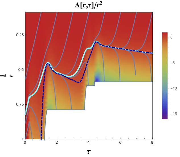
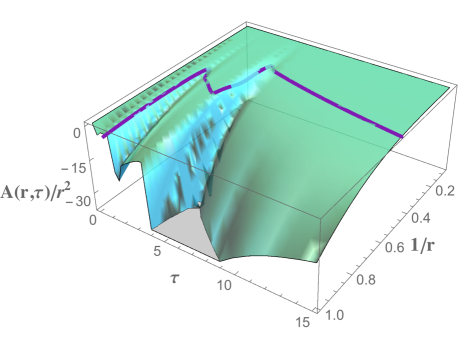
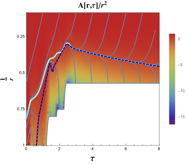
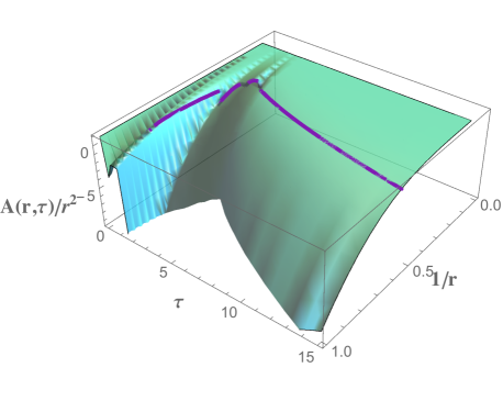
Figure 1: Model $\cal A$. The left panel shows the function $A(r,\tau)/r^{2}$, vs $\tau$ and $1/r$, obtained solving the Einstein equations (6)-(10) in the case of two distant (top panel) or close pulses (bottom panel) in the boundary metric. The color bar indicates the values of the function. The gray lines are radial null outgoing geodesics, the dashed dark blue line is the apparent horizon, and the continuous cyan line is the event horizon obtained as the critical geodesic. The excision in the low-$r$ region, used in the calculation, is shown. In the right panels, the 3d representation of $A(r,\tau)/r^{2}$ is displayed together with the apparent horizon (continuous line).

We can now discuss the three considered models, focusing on the effects of the boundary distortion and on the transient from the far-from-equilibrium state to the hydrodynamic regime.

Model $\cal A$.

In the case of two distant pulses, the horizon is formed as a two-step process which follows the sequence of the boundary distortion, as one can infer considering the computed function $A(r,\tau)/r^{2}$ which is depicted in Fig. 1. The outgoing radial null geodesics are clearly separated by a critical geodesic, the event horizon, which starts plunging back in the bulk immediately after each pulse in the boundary. This can be even more clearly seen in the plot of the $\tau$ dependence of the effective temperature $T_{eff}(\tau)$ and in the plot of the area of the apparent horizon per unit of rapidity, $\Sigma(r_{h},\tau)^{3}$, collected in Fig. 2. The temperature has two decreasing regimes, the first one after the first pulse, with the system starting relaxation immediately after the end of the boundary distortion. Time intervals of about twice the duration of the pulse are very long with respect to the relaxation time. The same phenomenon is observed considering the function $\Sigma(r_{h},\tau)^{3}$, which shows two time ranges in which it reaches a constant value, soon after the pulses. However, on such time scales, the components of the stress energy tensor have their own (computed) behavior, and no isotropization is observed after the first pulse.

On the other hand, for a distortion represented by two close (nearly overlapping) pulses, no particular structure is observed before the end of the boundary perturbation. The horizon area per unit of rapidity, $\Sigma(r_{h},\tau)^{3}$, has a sharp increase during the distortion, and reaches the asymptotic large $\tau$ value $\Sigma(r_{h},\tau)^{3}=\pi^{3}\Lambda^{2}$ soon after the end of the distortion.

The hydrodynamic $\tau-$dependence of $T_{eff}(\tau)$ and of the energy density $\epsilon(\tau)$, Eqs. (30) and (31), is reached immediately after the end of the distortion of the boundary $\tau_{f}^{A}$, with values of the parameter $\Lambda$ which are different for the two cases of different time intervals between the pulses. The values of $\Lambda$ obtained from $T_{eff}(\tau)$ are collected in Table 1. The temperature can be obtained from the condition $\dot{\Sigma}(r_{h},\tau)=0$, or from the energy density Eq.(29), with numerical results differing at the level of $2\%$. For a quantitative discussion, a time $\tau^{*}$ can be fixed imposing that the energy density $\epsilon(\tau^{*})$ differs from the hydrodynamic value $\epsilon_{H}(\tau^{*})$ in (31) by less than $5\%$:

$$\Big{|}\frac{\epsilon(\tau^{*})-\epsilon_{H}(\tau^{*})}{\epsilon(\tau^{*})}\Big{|}=0.05\,.$$ (39)

In both cases of distant or overlapping pulses, $\tau^{*}$ essentially coincides with the end of the boundary metric distortion. From the plot of $T^{\mu}_{\nu}$ in Fig. 3, we observe that at $\tau^{*}$ the pressure anisotropy is still sizeable, and the values of $\Delta p/\epsilon$ and $p_{||}/p_{\perp}$ are still much larger than the ones expected by viscous hydrodynamics. Therefore, we define the ”thermalization time” $\tau_{p}$ from the condition

$$\Big{|}\frac{p_{||}(\tau_{p})/p_{\perp}(\tau_{p})-(p_{||}(\tau_{p})/p_{\perp}(\tau_{p}))_{H}}{p_{||}(\tau_{p})/p_{\perp}(\tau_{p})}\Big{|}=0.05\,\,\,,$$ (40)

where $(p_{||}(\tau_{p})/p_{\perp}(\tau_{p}))_{H}$ is given by (34). Quantitatively, from the condition that $p_{\parallel}/p_{\perp}$ differs by less than $5\%$ from the asymptotic NNLO expression, we can set $\tau_{p}=6.8$ for two distant pulses. The difference $\tau_{p}-\tau^{*}$ can be expressed in physical units if one scale in the system is set. Imposing $T_{eff}(\tau^{*})=500$ MeV corresponds to $\tau_{p}-\tau^{*}\simeq 0.60$ fm/c, which indicates the elapsed time between the end of the pulse and the restoration of the hydrodynamical regime. For two overlapping pulses, the time difference is $\tau_{p}-\tau^{*}\simeq 1.03$ fm/c. The numerical values are collected in Table 1. Notice that $\tau^{*}$ and $\tau_{p}$ differ in general, although Eqs. (27) and (28) hold. Indeed, at a generic $\tau$ the relation between energy density and its asymptotic limit can be written as:

$$\epsilon(\tau)=\xi(\tau)\epsilon_{H}(\tau)\,\,,$$ (41)

with $\xi(\tau^{*})$ such that (39) is verified. For, e.g., the longitudinal pressure, using (27) and (41) one has $p_{\parallel}(\tau^{*})=\xi(\tau^{*})\,p_{\parallel,\,H}(\tau^{*})-\tau^{*}\,\xi^{\prime}(\tau^{*})\epsilon_{H}(\tau^{*})$. Therefore, due to the last term, the value $\tau_{p}$ verifying (40) does not necessarily coincide with $\tau^{*}$.

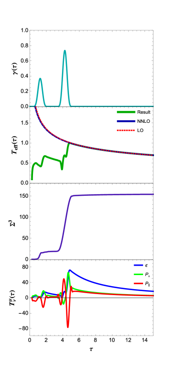
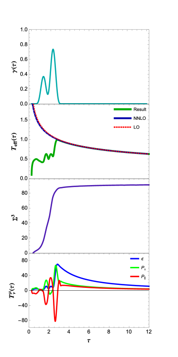
Figure 2: Model $\cal A$. The panels, for the profile $\gamma(\tau)$ with different time intervals between the pulses (left and right columns), show (from top to bottom) the function $\gamma(\tau)$, temperature $T_{eff}(\tau)$, horizon area $\Sigma^{3}(r_{h},\tau)$ per unit of rapidity, and the three components $\epsilon(\tau)$, $p_{\perp}(\tau)$ and $p_{\parallel}(\tau)$ of the stress-energy tensor $T^{\mu}_{\nu}$ (apart from the factor $\frac{N_{c}^{2}}{2\pi^{2}}$ ).

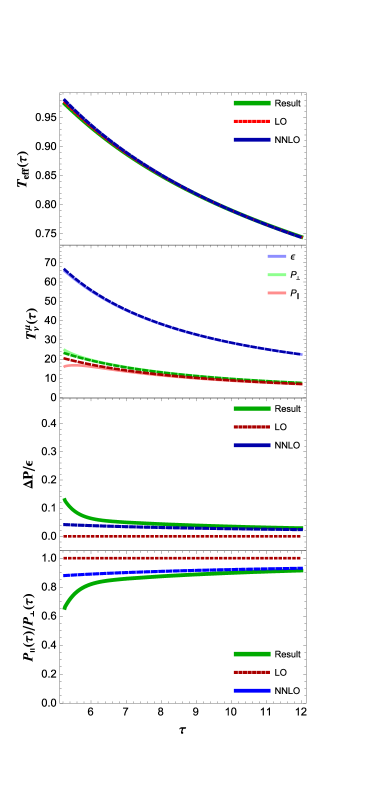
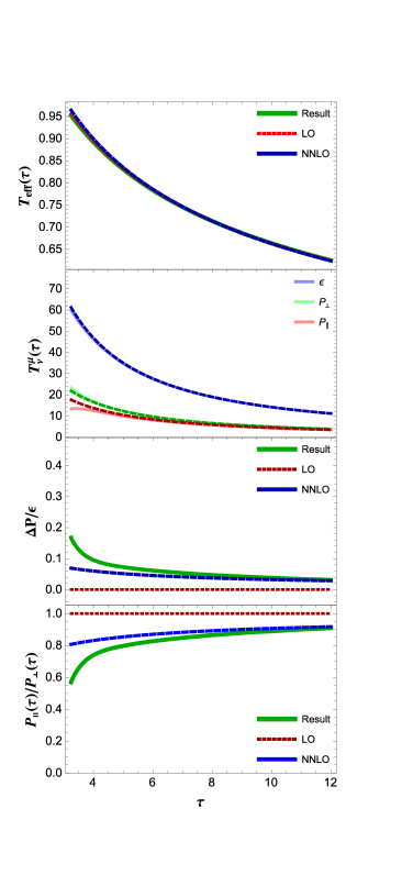
Figure 3: Model $\cal A$. From top to bottom: temperature $T_{eff}(\tau)$, components $\epsilon(\tau)$, $p_{\perp}(\tau)$ and $p_{\parallel}(\tau)$ of the stress-energy tensor, pressure anisotropy $\Delta p/\epsilon=(p_{\perp}-p_{\parallel})/\epsilon$ and ratio $p_{\parallel}/p_{\perp}$, computed for $\tau>\tau_{f}^{\cal A}$, for the boundary distortion with two distant (left) and two overlapping pulses (right panels). The short and long dashed lines correspond to the hydrodynamic result and to the NNLO result in the $1/\tau$ expansion.

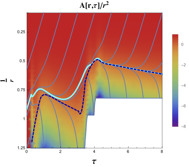
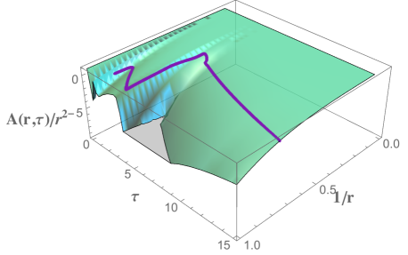
Figure 4: Model $\cal B$. Function $A(r,\tau)/r^{2}$, vs $\tau$ and $1/r$, outgoing radial null geodesics, event horizon and apparent horizon. Lines and colours have the same meaning as in Fig. 1.

Model $\cal B$.

The purpose of this model is to investigate a boundary distortion characterized by two largely different time scales. The horizon is formed immediately after the boundary deformation is switched on, as depicted in Fig. 4, then starts plugging down in the bulk until the short pulse becomes active. This can be seen clearly in Fig. 5, where the effective temperature and $\Sigma^{3}$ display a decreasing and constant regime, respectively, in the proper time interval $\tau_{i}<\tau<\tau_{0,1}$, after which a violent perturbation takes the system out of equilibrium. The time $\tau^{*}$ can be fixed using (31). For $\tau>\tau^{*}\simeq\tau_{f}^{\cal B}$ the determination of $\Lambda$ from $T_{eff}$ and the energy density $\epsilon$ gives $\Lambda=1.12$, with a variation of $3\%$ around this value. Thermalization is reached at the time $\tau_{p}$ obtained by the condition (40), as one can infer considering the observables depicted in Figs. 5 and 6. Setting the scale so that the temperature is $T_{eff}(\tau^{*})=500$ MeV, we find $\tau_{p}-\tau^{*}\simeq 0.42$ fm/c.

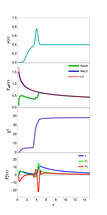
Figure 5: Model $\cal B$. The panels show (from top to bottom) the profile $\gamma(\tau)$, temperature $T_{eff}(\tau)$, horizon area per unit of rapidity $\Sigma^{3}(r_{h},\tau)$, and the three components $\epsilon(\tau)$, $p_{\perp}(\tau)$ and $p_{\parallel}(\tau)$ of $T^{\mu}_{\nu}$.

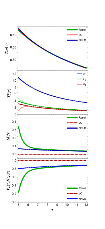
Figure 6: Model $\cal B$. From top to bottom: temperature $T_{eff}(\tau)$, components $\epsilon(\tau)$, $p_{\perp}(\tau)$ and $p_{\parallel}(\tau)$ of the stress-energy tensor, pressure anisotropy $\Delta p/\epsilon=(p_{\perp}-p_{\parallel})/\epsilon$ and ratio $p_{\parallel}/p_{\perp}$, computed for $\tau>\tau_{f}^{\cal B}$. The dashed lines correspond to the NNLO expressions.

Model $\cal C$.

This model is constructed with the aim of representing a situation close to the physical system during the scattering process, with two different time scales and several pulses of various number and intensity. Immediately after switching on the boundary deformation, the horizon is formed in the bulk geometry and follows the profile of the distortion. Even in short time intervals between the pulses, the horizon starts to plung in the bulk, with a decreasing temperature and a saturation of $\Sigma^{3}$. This can be inferred considering the computed function $A/r^{2}$ depicted in Fig. 7 and, in details, studying the $\tau$ dependence of the effective temperature and horizon area per unit rapidity in Fig. 8. $\Sigma^{3}(r_{h},\tau)$ displays a step-like behavior in proper time, closely following the distortion $\gamma(\tau)$, and reaches a constant value from $\tau=\tau_{f}^{\cal C}$ on. On the contrary, the various components of the stress-energy tensor have structures which become regular only for $\tau>\tau_{f}^{\cal C}$, after the last pulse. As one can observe analyzing the results in Fig. 9, the energy density reaches the NNLO hydrodynamic behavior at $\tau=\tau^{*}\simeq\tau_{f}^{\cal C}$, while pressure anisotropy persists for longer times. The parameter $\Lambda$, obtained from different observables, takes the value $\Lambda=1.59$, with a variation similar to the one in models $\cal A$ and $\cal B$. The pressure anisotropy $\Delta p/\epsilon$ and ratio $p_{\parallel}/p_{\perp}$ set the value $\tau_{p}$ of proper time, as one can infer considering the results in Fig. 9; setting $T_{eff}(\tau^{*})=500$ MeV, we obtain $\tau_{p}-\tau^{*}\simeq 0.2$ fm/c.

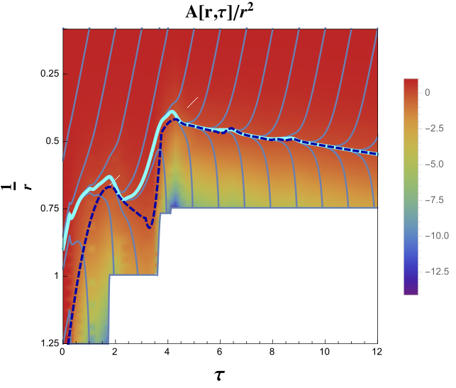
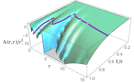
Figure 7: Model $\cal C$. Function $A(r,\tau)/r^{2}$, vs $\tau$ and $1/r$, outgoing radial null geodesics, events horizon and apparent horizon. The lines and colors are indicated as in Fig. 1.

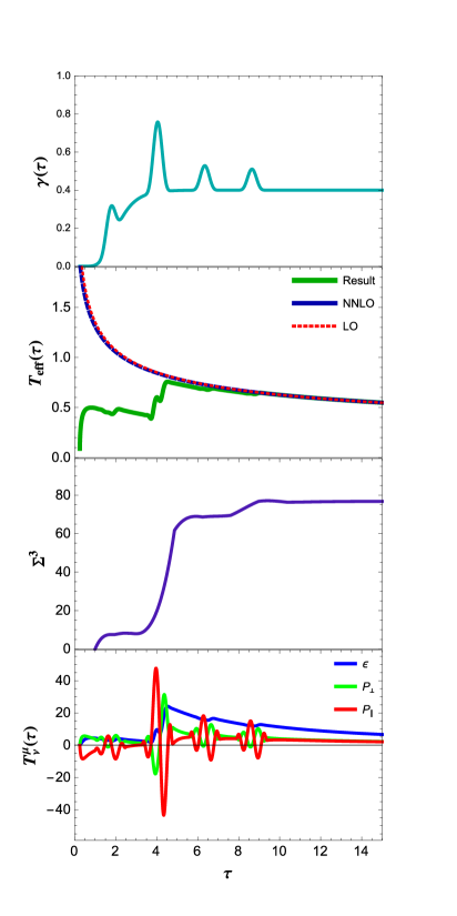
Figure 8: Model $\cal C$. From top to bottom: profile $\gamma(\tau)$, temperature $T_{eff}(\tau)$, horizon area per unit of rapidity $\Sigma^{3}(r_{h},\tau)$, and the three components $\epsilon(\tau)$, $p_{\perp}(\tau)$ and $p_{\parallel}(\tau)$ of $T^{\mu}_{\nu}$.

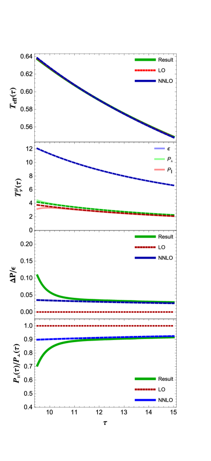
Figure 9: Model $\cal C$. From top to bottom: temperature $T_{eff}(\tau)$, components $\epsilon(\tau)$, $p_{\perp}(\tau)$ and $p_{\parallel}(\tau)$ of the stress-energy tensor, pressure anisotropy $\Delta p/\epsilon=(p_{\perp}-p_{\parallel})/\epsilon$ and ratio $p_{\parallel}/p_{\perp}$, computed for $\tau>\tau_{f}^{\cal B}$. The curves have the same meaning as in Fig. 6.

model	$\tau^{*}$	$\tau_{p}$	$\Lambda$	$\Delta\tau=\tau_{p}-\tau^{*}$ (fm/c)
${\cal A}~{}(1)$	5.25	6.8	2.25	0.60
${\cal A}~{}(2)$	3.25	6.0	1.73	1.03
${\cal B}$	5	6.74	1.12	0.42
${\cal C}$	9.45	10.24	1.59	0.20

Table 1: Numerical values of the relevant quantities for models $\cal A$, $\cal B$ and $\cal C$ of boundary distortion.

5 Conclusions

We have investigated the effects of different types of distortions of the boundary metric, in a boost-invariant setup. The quenches are introduced as a way to take the boundary theory out-of-equilibrium, and the distortion profiles are used to describe processes with different time scales and intensities. As a common feature, we observe a rapid formation of the horizon in the bulk metric, with the possibility of defining an effective $\tau-$dependent temperature. In coincidence with the end of each main distortion, the relaxation starts with the horizon plunging in the bulk. We have seen how sequences of distortions break the relaxation process. We find that for all the considered distortion profiles, $T_{eff}(\tau)$ starts to follow a viscous hydrodynamic expression as soon as the quench is switched off. At this time the pressures are different, and evolve towards a common value which is reached at a later time. Setting $T_{eff}(\tau^{*})=500$ MeV, the elapsed time before the restoration of the hydrodynamic regime is always a fraction of fm/c. Although the system described by the holographic approach is in several respects different from the real QCD system, and boundary sourcing a quite abstract representation of the heavy ion collision process, the obtained results allow us to argue what can be expected in realistic situations.

Acknowledgments.
We thank Giuseppe Eugenio Bruno and Marco Ruggieri for discussion. LB and PC thank the Galileo Galilei Institute for Theoretical Physics for the hospitality and the INFN for partial support during the completion of this work.

Appendix A Boundary stress-energy tensor

For the sake of completeness, we briefly describe the main steps of the calculation of the boundary stress-energy tensor $T^{\mu}_{\nu}$ leading to Eqs.(36)-(38). The $5D$ metric (14) can be written in ADM form [32],

$$ds^{2}=N^{2}dr^{2}+h_{\mu\nu}\left(dy^{\mu}+\mathcal{N}^{\mu}dr\right)\left(dy^{\nu}+\mathcal{N}^{\nu}dr\right)$$ (42)

in terms of the induced metric $h_{\mu\nu}$, of the lapse function $N$ and of the shift vector field $\mathcal{N}^{\mu}$. The stress tensor for the space foliation $\mathcal{M}_{r}$ obtained at constant $r$, is given by

$$\left.\tilde{T}^{\mu\nu}\right|_{r}=\frac{2}{\sqrt{|h|}}\left.\frac{\delta S}{\delta h_{\mu\nu}}\right|_{r},$$ (43)

with $h\equiv det\left(h_{\mu\nu}\right)$ and $S$ the gravitational action. The boundary stress energy tensor is obtained from the limit:

$$T^{\mu\nu}=\left.\lim_{r\to\infty}r^{2}\tilde{T}^{\mu\nu}\right|_{r}.$$ (44)

The action $S$ in (43) includes as a counterterm a local functional $S_{ct}$ of $h_{\mu\nu}$, whose contribution to $\tilde{T}^{\mu\nu}$ regularizes the divergences at $r\to\infty$ [33],[31]. As a consequence, the stress-energy tensor is written as

$$T^{\mu\nu}=\lim_{r\to\infty}\frac{N_{c}^{2}}{4\pi^{2}}\,r^{2}\left(K^{\mu\nu}-Kh^{\mu\nu}-3h^{\mu\nu}+\frac{1}{2}{\,}^{(4)}G^{\mu\nu}-\sigma^{\mu\nu}\frac{1}{r^{2}}\log r\right),$$ (45)

with $K^{\mu\nu}$ the extrinsic curvature, ${\,}^{(4)}G^{\mu\nu}$ the boundary Einstein tensor with curvature tensors defined with respect to $h_{\mu\nu}$. The counterterms $-3h^{\mu\nu}+\frac{1}{2}{\,}^{(4)}G^{\mu\nu}$ cancel the powers from $r^{2}$ to $r^{-1}$ from the first two terms in (45), and introduce terms of order $r^{-2}$ which contribute to the final result (45) [33]. The last term proportional to $\sigma^{\mu\nu}$, with in our case

$$\sigma_{\mu\nu} = diag\left\{-\frac{3}{2}\alpha_{4}(\tau),e^{\gamma(\tau)}\left[-\frac{1}{2}\alpha_{4}(\tau)+2\beta_{4}(\tau)\right],\right.$$ (46)

$$\left.e^{\gamma(\tau)}\left[-\frac{1}{2}\alpha_{4}(\tau)+2\beta_{4}(\tau)\right],e^{-2\gamma(\tau)}\tau^{2}\left[-\frac{1}{2}\alpha_{4}(\tau)-4\beta_{4}(\tau)\right]\right\}\,\,\,$$

and $\alpha_{4}(\tau)$ and $\beta_{4}(\tau)$ in (15)-(17), cancels the $\frac{1}{r^{2}}\log r$ contributions in (45). The results for the components of the stress-energy tensor Eq. (1) are in Eqs.(36)-(38), with:

$$\tilde{\epsilon}_{\gamma} = \frac{25}{144}\frac{\gamma^{\prime}}{\tau^{3}}-\frac{\frac{65}{96}\gamma^{\prime 2}+\frac{25}{144}\gamma^{\prime\prime}}{\tau^{2}}+\frac{\frac{19}{32}\gamma^{\prime 3}+\frac{1}{96}\gamma^{\prime}(\tau)\gamma^{\prime\prime}-\frac{5}{48}\gamma^{(3)}}{\tau}-\frac{57}{256}\gamma^{\prime 4}-\frac{1}{8}\gamma^{\prime\prime 2}+\frac{5}{32}\gamma^{\prime}\gamma^{(3)}\,,$$

$$\tilde{p}_{\perp\,\gamma} = -\frac{1}{6\tau^{4}}+\frac{409}{576}\frac{\gamma^{\prime}}{\tau^{3}}-\frac{\frac{8}{9}\gamma^{\prime 2}+\frac{587}{1728}\gamma^{\prime\prime}}{\tau^{2}}+\frac{\frac{73}{192}\gamma^{\prime 3}+\frac{145}{288}\gamma^{\prime}(\tau)\gamma^{\prime\prime}-\frac{1}{288}\gamma^{(3)}}{\tau}$$ (48)

$$- \frac{11}{256}\gamma^{\prime 4}-\frac{21}{64}\gamma^{\prime 2}\gamma^{\prime\prime}-\frac{1}{96}\gamma^{\prime\prime 2}+\frac{5}{96}\gamma^{\prime}\gamma^{(3)}+\frac{7}{192}\gamma^{(4)}\,,$$

$$\tilde{p}_{\|\,\gamma} = \frac{1}{3\tau^{4}}-\frac{359}{288}\frac{\gamma^{\prime}}{\tau^{3}}+\frac{\frac{49}{36}\gamma^{\prime 2}+\frac{437}{864}\gamma^{\prime\prime}}{\tau^{2}}-\frac{\frac{5}{12}\gamma^{\prime 3}+\frac{233}{288}\gamma^{\prime}\gamma^{\prime\prime}+\frac{7}{72}\gamma^{(3)}}{\tau}$$ (49)

$$- \frac{11}{256}\gamma^{\prime 4}+\frac{21}{32}\gamma^{\prime 2}\gamma^{\prime\prime}-\frac{1}{96}\gamma^{\prime\prime 2}+\frac{5}{96}\gamma^{\prime}\gamma^{(3)}-\frac{7}{96}\gamma^{(4)}\,.$$

Energy density and pressures are hence affected by the variations of $\gamma(\tau)$. The above expressions coincide (after the correction of an overall minus sign in $\tilde{\epsilon}_{\gamma}$) with the ones in [12] after the recognition of terms due to the regularization scheme proportional to $\sigma_{\mu\nu}$, related to the coefficient of the $r^{-4}\log[r]$ term in the large-$r$ expansion of the metric. The covariant conservation of the stress-energy tensor gives again Eq. (21).

Appendix B Testing the numerical algorithm

To quantify the accuracy of our numerical algorithm, based on the Runge-Kutta method for the solution of the differential equations in the variable $r$, we monitor the ratios

$${\cal R}_{6}(r,\tau) = \frac{\Sigma({\dot{\Sigma}})^{\prime}+2\Sigma^{\prime}{\dot{\Sigma}}-2\Sigma^{2}}{|\Sigma({\dot{\Sigma}})^{\prime}|+2|\Sigma^{\prime}{\dot{\Sigma}}|+2|\Sigma^{2}|}$$ (50)

$${\cal R}_{7}(r,\tau) = \frac{\Sigma({\dot{B}})^{\prime}+\frac{3}{2}\left(\Sigma^{\prime}{\dot{B}}+B^{\prime}{\dot{\Sigma}}\right)}{|\Sigma({\dot{B}})^{\prime}|+\frac{3}{2}\left(|\Sigma^{\prime}{\dot{B}}|+|B^{\prime}{\dot{\Sigma}}|\right)}$$ (51)

$${\cal R}_{8}(r,\tau) = \frac{A^{\prime\prime}+3B^{\prime}{\dot{B}}-12\frac{\Sigma^{\prime}{\dot{\Sigma}}}{\Sigma^{2}}+4}{|A^{\prime\prime}|+3|B^{\prime}{\dot{B}}|+|12\frac{\Sigma^{\prime}{\dot{\Sigma}}}{\Sigma^{2}}|+4}$$ (52)

$${\cal R}_{9}(r,\tau) = \frac{{\ddot{\Sigma}}+\frac{1}{2}\left({\dot{B}}^{2}\Sigma-A^{\prime}{\dot{\Sigma}}\right)}{|{\ddot{\Sigma}}|+\frac{1}{2}\left(|{\dot{B}}^{2}\Sigma|+|A^{\prime}{\dot{\Sigma}}|\right)}$$ (53)

$${\cal R}_{10}(r,\tau) = \frac{\Sigma^{\prime\prime}+\frac{1}{2}B^{\prime 2}\Sigma}{|\Sigma^{\prime\prime}|+\frac{1}{2}B^{\prime 2}|\Sigma|}\,\,$$ (54)

in the $(r,\,\tau)$ domain behind the excision $r>r_{min}$. The final results are shown in Fig. 10 in the case of model $\cal B$.

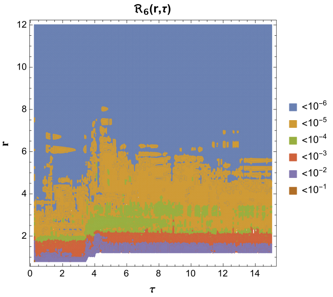
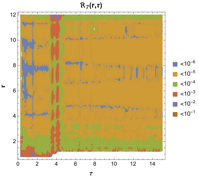
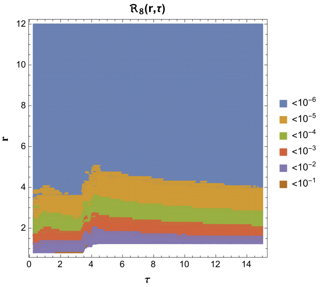
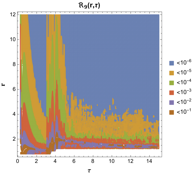
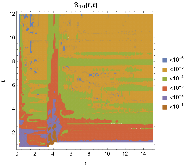
Figure 10: Ratios ${\cal R}_{i}(r,\tau)$ in the case of model $\cal B$. The white region corresponds to the excision in $r_{min}$ .

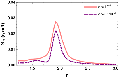
Figure 11: Ratio ${\cal R}_{9}(r,\tau=4)$ computed in the range $1.2\leqslant r\leqslant 3.0$ for $d\tau=10^{-2}$ (pink, continuous curve) and $d\tau=0.5\cdot 10^{-2}$ (purple, dashed curve) in the case of model $\cal B$ .

The resulting ratios ${\cal R}_{6},\,{\cal R}_{7},\,{\cal R}_{8}$ deviate from zero at a level smaller than ${\cal O}(10^{-4})$, but for a tiny region close to the excision in the case of ${\cal R}_{6}$ and ${\cal R}_{8}$, and for a few spots in the range $3\leqslant r\leqslant 5$ (where the source function $\gamma(\tau)$ is peaked) in the case of ${\cal R}_{7}$. A similar result is obtained for ${\cal R}_{9}$ and ${\cal R}_{10}$, with larger deviations from zero: this is a consequence, for ${\cal R}_{10}$, of the smallness of the two addendi in (10), and for ${\cal R}_{9}$ of the computation of ${\ddot{\Sigma}}=\partial_{\tau}{\dot{\Sigma}}+\frac{1}{2}A\,(\dot{\Sigma})^{\prime}$ through a discretized time derivative. To monitor the time slicing, we compute ${\cal R}_{9}$ for two different time steps in the region $1.2\leqslant r\leqslant 3.0$ at $\tau=4$, where there is the largest deviation from zero. Comparing the results for $d\tau=10^{-2}$ and $d\tau=0.5\cdot 10^{-2}$, as shown in Fig. 11, one observes the decreasing of ${\cal R}_{9}$ by doubling the grid points.

References

- [1] J. M. Maldacena, The Large N limit of superconformal field theories and supergravity, Int.J.Theor.Phys. 38 (1999) 1113–1133, [hep-th/9711200].
- [2] E. Witten, Anti-de Sitter space and holography, Adv.Theor.Math.Phys. 2 (1998) 253–291, [hep-th/9802150].
- [3] S. Gubser, I. R. Klebanov, and A. M. Polyakov, Gauge theory correlators from noncritical string theory, Phys.Lett. B428 (1998) 105–114, [hep-th/9802109].
- [4] V. E. Hubeny and M. Rangamani, A Holographic view on physics out of equilibrium, Adv.High Energy Phys. 2010 (2010) 297916, [arXiv:1006.3675].
- [5] U. W. Heinz, Thermalization at RHIC, AIP Conf.Proc. 739 (2005) 163–180, [nucl-th/0407067].
- [6] E. Shuryak, Heavy Ion Collisions: Achievements and Challenges, arXiv:1412.8393.
- [7] T. Epelbaum and F. Gelis, Pressure isotropization in high energy heavy ion collisions, Phys.Rev.Lett. 111 (2013) 232301, [arXiv:1307.2214].
- [8] J. Casalderrey-Solana, H. Liu, D. Mateos, K. Rajagopal, and U. A. Wiedemann, Gauge/String Duality, Hot QCD and Heavy Ion Collisions, arXiv:1101.0618.
- [9] S. Bhattacharyya, V. E. Hubeny, S. Minwalla, and M. Rangamani, Nonlinear Fluid Dynamics from Gravity, JHEP 0802 (2008) 045, [arXiv:0712.2456].
- [10] R. A. Janik and R. B. Peschanski, Asymptotic perfect fluid dynamics as a consequence of Ads/CFT, Phys.Rev. D73 (2006) 045013, [hep-th/0512162].
- [11] P. M. Chesler and L. G. Yaffe, Horizon formation and far-from-equilibrium isotropization in supersymmetric Yang-Mills plasma, Phys.Rev.Lett. 102 (2009) 211601, [arXiv:0812.2053].
- [12] P. M. Chesler and L. G. Yaffe, Boost invariant flow, black hole formation, and far-from-equilibrium dynamics in N = 4 supersymmetric Yang-Mills theory, Phys.Rev. D82 (2010) 026006, [arXiv:0906.4426].
- [13] M. P. Heller, R. A. Janik, and P. Witaszczyk, The characteristics of thermalization of boost-invariant plasma from holography, Phys.Rev.Lett. 108 (2012) 201602, [arXiv:1103.3452].
- [14] M. P. Heller, R. A. Janik, and P. Witaszczyk, A numerical relativity approach to the initial value problem in asymptotically Anti-de Sitter spacetime for plasma thermalization - an ADM formulation, Phys.Rev. D85 (2012) 126002, [arXiv:1203.0755].
- [15] M. P. Heller, D. Mateos, W. van der Schee, and D. Trancanelli, Strong Coupling Isotropization of Non-Abelian Plasmas Simplified, Phys.Rev.Lett. 108 (2012) 191601, [arXiv:1202.0981].
- [16] B. Wu and P. Romatschke, Shock wave collisions in AdS5: approximate numerical solutions, Int.J.Mod.Phys. C22 (2011) 1317–1342, [arXiv:1108.3715].
- [17] M. P. Heller, D. Mateos, W. van der Schee, and M. Triana, Holographic isotropization linearized, JHEP 1309 (2013) 026, [arXiv:1304.5172].
- [18] J. Jankowski, G. Plewa, and M. Spalinski, Statistics of thermalization in Bjorken Flow, JHEP 1412 (2014) 105, [arXiv:1411.1969].
- [19] D. Grumiller and P. Romatschke, On the collision of two shock waves in AdS(5), JHEP 0808 (2008) 027, [arXiv:0803.3226].
- [20] P. M. Chesler and L. G. Yaffe, Holography and colliding gravitational shock waves in asymptotically AdS5 spacetime, Phys.Rev.Lett. 106 (2011) 021601, [arXiv:1011.3562].
- [21] W. van der Schee, P. Romatschke, and S. Pratt, Fully Dynamical Simulation of Central Nuclear Collisions, Phys.Rev.Lett. 111 (2013), no. 22 222302, [arXiv:1307.2539].
- [22] P. M. Chesler and L. G. Yaffe, Holography and off-center collisions of localized shock waves, arXiv:1501.0464.
- [23] P. M. Chesler and L. G. Yaffe, Numerical solution of gravitational dynamics in asymptotically anti-de Sitter spacetimes, JHEP 1407 (2014) 086, [arXiv:1309.1439].
- [24] J. York, in Frontiers in Numerical Relativity. C.R. Evans, L.S. Finn, and D.W. Hobill (eds), Chicago University Press, 2011.
- [25] S. Bhattacharyya, V. E. Hubeny, R. Loganayagam, G. Mandal, S. Minwalla, et. al., Local Fluid Dynamical Entropy from Gravity, JHEP 0806 (2008) 055, [arXiv:0803.2526].
- [26] I. Booth, M. P. Heller, and M. Spalinski, Black brane entropy and hydrodynamics: The Boost-invariant case, Phys.Rev. D80 (2009) 126013, [arXiv:0910.0748].
- [27] J. Bjorken, Highly Relativistic Nucleus-Nucleus Collisions: The Central Rapidity Region, Phys.Rev. D27 (1983) 140–151.
- [28] M. P. Heller and R. A. Janik, Viscous hydrodynamics relaxation time from AdS/CFT, Phys.Rev. D76 (2007) 025027, [hep-th/0703243].
- [29] R. Baier, P. Romatschke, D. T. Son, A. O. Starinets, and M. A. Stephanov, Relativistic viscous hydrodynamics, conformal invariance, and holography, JHEP 0804 (2008) 100, [arXiv:0712.2451].
- [30] S. de Haro, S. N. Solodukhin, and K. Skenderis, Holographic reconstruction of space-time and renormalization in the AdS / CFT correspondence, Commun.Math.Phys. 217 (2001) 595–622, [hep-th/0002230].
- [31] S. Kinoshita, S. Mukohyama, S. Nakamura, and K.-y. Oda, A Holographic Dual of Bjorken Flow, Prog.Theor.Phys. 121 (2009) 121–164, [arXiv:0807.3797].
- [32] R. L. Arnowitt, S. Deser, and C. W. Misner, The Dynamics of general relativity, Gen.Rel.Grav. 40 (2008) 1997–2027, [gr-qc/0405109].
- [33] V. Balasubramanian and P. Kraus, A Stress tensor for Anti-de Sitter gravity, Commun.Math.Phys. 208 (1999) 413–428, [hep-th/9902121].