Parareal multiscale methods for highly oscillatory dynamical systems

Abstract

We introduce a new strategy for coupling the parallel in time (parareal) iterative methodology with multiscale integrators. Following the parareal framework, the algorithm computes a low-cost approximation of all slow variables in the system using an appropriate multiscale integrator, which is refined using parallel fine scale integrations. Convergence is obtained using an alignment algorithm for fast phase-like variables. The method may be used either to enhance the accuracy and range of applicability of the multiscale method in approximating only the slow variables, or to resolve all the state variables. The numerical scheme does not require that the system is split into slow and fast coordinates. Moreover, the dynamics may involve hidden slow variables, for example, due to resonances. We propose an alignment algorithm for almost-periodic solution, in which case convergence of the parareal iterations is proved. The applicability of the method is demonstrated in numerical examples.

1 Introduction

The parallel in time, also known as the “parareal” method, introduced by Lions, Maday and Turinici [49] is a simple yet effective scheme for the parallelization of numerical solutions for a large class of time dependent problems [50]. It consists of a fixed point iteration involving a coarse-but-cheap and a fine-but-expensive integrators. Computational time is reduced by parallelization of the fine integrations. For problems with separated multiple scales, it is tempting to apply a multiscale solver as a coarse integrator. So far, such types of parallel methods are limited to a few special multiscale cases such as chemical kinetics [16, 23, 33], dissipative ordinary differential equations (ODEs) [47] and highly oscillatory (HiOsc) problems in which the oscillatory behavior is relatively simple [20, 32]. One difficulty stems out from a fundamental difference between the parareal and the multiscale philosophies — while the former requires point-wise convergence of the numerical solvers (in the state variable), most multiscale schemes gain efficiency by only approximating a reduced set of slowly varying coarse/slow/macroscopic variables [10, 11, 22, 29, 41, 55].

In this paper, we develop a general strategy that couples multiscale integrators and fully resolved fine scale integration for parallel in time computation of HiOsc solutions of a class of ODEs. There are several advantages in such coupling strategies. First, some multiscale methods (such as the Poincaré-map technique [2]) only approximate the slow constituents or slow variables of the dynamics. Proper coupling of multiscale and fine scale solvers via a parareal-like framework can be efficient (by parallelization) in computing full detailed solutions, including the fast phase in the HiOsc dynamics. The choice of multiscale method is not limited to the Poincaré-map technique. Any multiscale method can be used as a coarse integrator as long as fast phase-like variables are appropriately aligned as required. Then, convergence of the parareal iterations can be shown in a similar manner. Second, the parareal iterations enhance the stability and accuracy of the multiscale scheme, in particular when the scale separation in the system is not significant and the corresponding sampling/averaging errors are non-negligible. Finally, parareal multiscale coupling schemes can deal with more challenging situations, for example, (a) the effective equation is valid almost everywhere macroscopically, but is not an adequate description of the system at small but a priori ”unpredictable” locations in the phase space (as these regions may depend on the solutions); and (b) the influence of microscopic solutions in these regions on the macroscopic solution elsewhere is significant.

In [47], Legoll et at suggest a multiscale parareal scheme for singularly perturbed ODEs in which the fast dynamics is dissipative, i.e., the dynamics relaxes rapidly to a low dimensional manifold. One of the main contributions of [47] is the understanding that the slow and fast parts of the dynamics need to be addressed separately. They suggest two approaches: The first is a straight-forward application of parareal, which is shown to converge but loses accuracy as the system becomes more singular. In Section 1.3 we demonstrate that naive parareal does not converge when applied for HiOsc systems. The second approach assumes that the system is split into slow and fast variables, or that a change of variables splitting the system is given. This approach may be applied to HiOsc systems, but it is relatively restrictive as in many examples and applications such a splitting is not known. Dai et al [20] suggest an application of the parareal framework to Hamiltonian systems. They consider two main approaches. The first is a time-reversible iteration scheme (applied together with time-reversible fine and coarse integrators). The second projects solutions at coarse time segments onto the constant energy manifold. The two approaches are also combined together. The first approach is specific to Hamiltonian dynamics and not to general HiOsc problems. The projection method cannot be applied to the HiOsc case because the main difficulty is not with the approximation of slow variables (or constants of motion), but with the fast phase. In addition, since the methods presented in [20] are not multiscale, their accuracy and efficiency are expected to deteriorate when the frequencies of oscillations are large. Combining the symmetric approach of Dai et al with our alignment method for Hamiltonian systems may be an interesting application, but is beyond the scope of the current manuscript. In particular, the alignment algorithms should also be made symmetric, similar to the ideas of Dai et al. Applications of parareal methods to Hamiltonian dynamics is also analyzed in [27]. Additional approaches to use symplectic integrators with applications to molecular dynamics include [12, 13, 38]. Finally, Haut and Wingate [32] suggest a parareal method for PDEs with linear HiOsc forcing, As in [47], their method applies exact knowledge of the fast variable (the phase in the HiOsc case) to design a convergent parareal scheme. In this respect, the method proposed here goes further and is also applicable to nonlinear HiOsc systems. However, in this paper the discussion is restricted to the ODE case. One of the main goals of the current paper is to design a convergent parareal algorithm that does not require explicit knowledge of the fast and slow variables.

We begin with a short overview of the parareal method within the context of ODEs and test its performance on a simple example HiOsc system.

1.1 The parareal method for ODEs

Consider the following initial value problem

$$\dot{u}=f(t,u),\leavevmode\nobreak\ \leavevmode\nobreak\ \leavevmode\nobreak\ u(0)=u_{0},$$ (1.1)

where $u\in\mathbb{R}^{d}$ and $t\in[0,T]$. We assume that $f$ is sufficiently smooth. Let $H$ denote an intermediate time step, $0<H<T$ and $N=T/H$ an integer. Suppose that we are given two approximate integrators for (1.1): a cheap coarse integrator with low accuracy denoted ${\mathcal{C}}$, and a fine, high accuracy integrator which is relatively expensive in terms of efficiency, denoted ${\mathcal{F}}$. The approximate propagation operators to time $H$ obtained using the the coarse and fine integrators are denoted by ${\mathcal{C}}_{H}$ and ${\mathcal{F}}_{H}$, respectively.

Furthermore, denote by $u^{k}_{n}$ the approximation for $u(nH)$ at the $k$’th iteration. For all iterations, the initial values are the same $\forall k,u^{k}_{0}=u_{0}$. The objective is to have $u^{k}_{n}\to{\mathcal{F}}_{nH}u_{0}$ as $k\to\infty$, i.e., convergence to the approximation given by the high-accuracy fine integrator. The parareal approximation to (1.1) is as follows. See Figure 1 for a sketch of the parareal methodology.

Algorithm 1.1.

1. Initialization: Construct the zero’th iteration approximation using a chosen coarse integrator:

   $$u_{0}^{0}=u_{0}\leavevmode\nobreak\ \leavevmode\nobreak\ {\rm and}\leavevmode\nobreak\ \leavevmode\nobreak\ u^{0}_{n}={\mathcal{C}}_{H}u^{0}_{n-1},\leavevmode\nobreak\ \leavevmode\nobreak\ \leavevmode\nobreak\ n=1,\dots,N.$$

2. Iterations: $k=1\dots K$

   $$u_{0}^{k}=u_{0}\leavevmode\nobreak\ \leavevmode\nobreak\ {\rm and}\leavevmode\nobreak\ \leavevmode\nobreak\ u_{n}^{k}={\mathcal{C}}_{H}u_{n-1}^{k}+{\mathcal{F}}_{H}u_{n-1}^{k-1}-{\mathcal{C}}_{H}u_{n-1}^{k-1},\leavevmode\nobreak\ \leavevmode\nobreak\ \leavevmode\nobreak\ n=1,\dots,N.$$ (1.2)

Note that the calculation of the fine integrator ${\mathcal{F}}_{H}u_{n-1}^{k-1}$ in (1.2) requires only the initial condition $u_{n-1}^{k-1}$, which depends on the previous iteration. Hence, for each $k$, $\mathcal{F}_{t}u^{k-1}_{n-1},$ $0<t\leq H$, $n=1,2,\cdots,N$ can be computed in parallel. The solution computed by the accurate but expensive integrator is a fixed point. Indeed, when the iteration is sufficiently large ($k\geq n$), the solution $u^{k}_{n}$ become identical to it:

$$u^{k}_{n}=\mathcal{F}_{nH}u_{0},\leavevmode\nobreak\ \leavevmode\nobreak\ \leavevmode\nobreak\ n\leq k.$$

In fact, (1.2) can be regarded as a fixed-point iteration. In [50], it is proved that under some sufficient conditions of $f$, which we shall recall in Section 1.2,

$$|u_{n}^{k}-u(nH)|\leq C(H^{k}+E_{f}),$$ (1.3)

where $E_{f}$ is the global error in solving the full ODE using the fine propagator, and $C$ depends on the derivatives of the solutions. Eq. (1.3) assumes a 1st order coarse integrator.

In order to identify the source of the difficulty in developing parareal algorithms for highly oscillatory problems, we adapt the parareal proof of convergence given by Maday in [50] for non-singular ODEs.

Figure 1: A sketch depicting the parareal methodology. Each parareal iteration is constructed using three integrations: Fine integration starting at $u_{n}^{k-1}$, coarse integration starting at $u_{n}^{k-1}$ and another coarse integration starting at $u_{n}^{k}$. The first two depend only on previous iterations and can therefore be computed in parallel.

1.2 Convergence of parareal

We consider ODEs of the form (1.1) with initial conditions $u(0)=u_{0}\in D\subset\mathbb{R}^{d}$. We are interested in solving (1.1) in a fixed time segment $[0,T]$. The solution is denoted $u(t;u_{0}),\;t\in[0,T]$. Let $\Phi$ denote the flow map (propagator) associated with (1.1),

$${\Phi}_{t}x=u(t;x),\leavevmode\nobreak\ \leavevmode\nobreak\ \forall t>0.$$

For sufficiently smooth $f$ we have that $\left|{\Phi}_{t}x-{\Phi}_{t}y\right|\leq e^{Ct}|x-y|$. In the following $C$ denotes a generic positive constant which may depend on $T$. Since $t\leq T$, the prefactor $e^{Ct}$ can be bounded by $1+T^{-1}e^{CT}t$. This yields a linear stability bound for ${\Phi}_{t}$,

$$\left|{\Phi}_{t}x-{\Phi}_{t}y\right|\leq(1+Ct)|x-y|.$$

For simplicity, we assume that the coarse integrator ${\mathcal{C}}_{t}$ is a one-step method with step size $H$ while the fine integrator ${\mathcal{F}}_{t}$ has step size $h\ll H$. In addition, we make the following accuracy and stability assumptions on the numerical integrators:

$$\left|{\mathcal{F}}_{t}x-{\Phi}_{t}x\right|\leq CtE_{f}(1+|x|),\;\;\left|{\mathcal{C}}_{t}x-{\Phi}_{t}x\right|\leq CtE_{c}(1+|x|)$$ (1.4)

where $E_{f}$ and $E_{c}$ denote the global sup error in solving (1.1) in $[0,T]$ using respectively the fine and coarse integrators in the entire domain of interest $D$. Note that both $E_{f}$ and $E_{c}$ typically depend on $T$. In addition,

$$\left|{\mathcal{F}}_{t}x-{\mathcal{F}}_{t}y\right|\leq(1+tC)|x-y|,\;\;\left|{\mathcal{C}}_{t}x-{\mathcal{C}}_{t}y\right|\leq(1+tC)|x-y|$$ (1.5)

Let $\delta{\mathcal{F}}_{t}={\Phi}_{t}-{\mathcal{F}}_{t}$ and $\delta{\mathcal{C}}_{t}={\Phi}_{t}-{\mathcal{C}}_{t}$, denote the errors in the fine and coarse propagators, respectively. Then, by a triangle inequality,

$$\left|\delta{\mathcal{F}}_{t}x-\delta{\mathcal{F}}_{t}y\right|\leq(1+tCE_{f})|x-y|,\;\;\left|\delta{\mathcal{C}}_{t}x-\delta{\mathcal{C}}_{t}y\right|\leq(1+tCE_{c})|x-y|.$$ (1.6)

We recite the following theorem from [50].

Theorem 1.2.

Let $K\leq N/2=T/2H$. Then, for all $k\leq K$,

$$\sup_{n=0,\dots,N}|u_{n}^{k}-{\mathcal{F}}_{nH}u_{0}|\leq C(E_{c})^{k}.$$

Consequently,

$$\sup_{n=0,\dots,N}|u_{n}^{k}-u(nH)|\leq C\left[(E_{c})^{k}+E_{f}\right].$$ (1.7)

Proof: Applying the parareal iterations (1.2),

$$u_{n}^{k}-{\mathcal{F}}_{nH}u_{0}= \left[{\mathcal{C}}_{H}u_{n-1}^{k}-{\mathcal{C}}_{H}u_{n-1}^{k-1}\right]+\left[{\mathcal{F}}_{H}u_{n-1}^{k-1}-{\mathcal{F}}_{H}{\mathcal{F}}_{(n-1)H}u_{0}\right]$$ (1.8)

$$= \left[{\mathcal{C}}_{H}u_{n-1}^{k}-{\mathcal{C}}_{H}{\mathcal{F}}_{(n-1)H}u_{0}\right]-\left[\delta{\mathcal{C}}_{H}\left({\mathcal{F}}_{(n-1)H}u_{0}\right)-\delta{\mathcal{C}}_{H}u_{n-1}^{k-1}\right]$$

$$-\left[\delta{\mathcal{F}}_{H}u_{n-1}^{k-1}-\delta{\mathcal{F}}_{H}\left({\mathcal{F}}_{(n-1)H}u_{0}\right)\right],$$

Using assumption (1.6), and denoting $\theta_{n}^{k}=C(1+CH)^{k-n}(E_{f}+E_{c})^{-k}H^{-k}\left|u_{n}^{k}-{\mathcal{F}}_{nH}u_{0}\right|,$ we have $\theta_{n}^{k}\leq\theta_{n-1}^{k}+\theta_{n-1}^{k-1}$. By induction, $\theta_{n}^{k}\leq C\left(\begin{array}[]{c}n\\ k\end{array}\right)$. Assuming that $E_{f}<E_{c}$,

$$\left|u_{n}^{k}-{\mathcal{F}}_{nH}u_{0}\right|\leq CT^{K}E_{c}^{k}={\mathcal{O}}(E_{c}^{k}).$$ (1.9)

1.3 Parareal and HiOsc ODEs

We consider HiOsc ODEs given in the singular perturbation form

$$\dot{u}=\epsilon^{-1}f_{1}(u)+f_{0}(u),$$ (1.10)

with initial condition $u(0)=u_{0}\in D\subset\mathbb{R}^{d}$, where $D$ is a domain uniformly bounded in $\epsilon$. The parameter $0<\epsilon\leq\epsilon_{0}\ll 1$ characterizes the separation of time scales – the fast scale involves oscillations with frequencies of order $\epsilon^{-1}$ while the computational time domain is $[0,T]$ with $T$ independent of $\epsilon$. Throughout the paper we assume that $f_{1},\;f_{0}$ are sufficiently smooth, and that for each $u_{0}\in D$, $u(t)$ is uniformly bounded in $\epsilon$ in the time interval $[0,T]$. Furthermore, we assume that the Jacobian of $f_{1}$ has only purely imaginary eigenvalues in $D$, which are bounded away from $0$ and independent of $\epsilon$. These settings typically imply that the computational complexity of direct non-multiscale methods is at least $\mathcal{O}(\epsilon^{-1})$.

To understand some of the challenges in applying the parareal framework to HiOsc systems, we consider the following simple example

$$\dot{u}=(\alpha+i\epsilon^{-1})u,\leavevmode\nobreak\ \leavevmode\nobreak\ \leavevmode\nobreak\ u(0)=1.$$ (1.11)

With $\alpha>0$, the trajectory of $u(t)=e^{(\alpha+i\epsilon^{-1})t}$ is an expanding spiral in the complex plane. We further assume that the fine integrator is exact, ${\mathcal{F}}_{t}u=e^{(\alpha+i\epsilon^{-1})t}u$. We first investigate the performance of Algorithm 1.1 using two conventional methods as $\mathcal{C}_{t}$: Implicit Euler, Explicit Euler, and Trapezoidal Rule. Table 1 compares the minimal number of parareal iterations, $K$, to reach an absolute error below $1/10$. We observe that when conventional methods are implemented as a coarse integrator $K$ becomes prohibitively large as $\epsilon$ gets small. The increase in $K$ for conventional coarse integrators can be explained by the error estimate (1.3). The difficulty lies in the constant $C$, which grows rapidly with $1/\epsilon$. For an order $p$ coarse integrator, the error is proportional to the $p+1$ time derivative of $f$, which is of order $\mathcal{O}(\epsilon^{-(p+1)})$. As a result, the parareal error for HiOsc systems (1.7) depends on $\epsilon$,

$$|u_{n}^{k}-u(nH)|\leq C\left\{E_{f}+\left[\epsilon^{-1}\left(\epsilon^{-1}H\right)^{p}\right]^{k}\right\}.$$ (1.12)

An immediate consequence is that $H$ has to be ${o}(\epsilon)$, even when applying A-stable or symplectic methods. See for example the conclusion in [20].

Coarse integrator	$\epsilon$=	0.2	0.1	0.05	0.02	0.01	0.001
Explicit Euler $(H=\epsilon/5)$	$K$	7	12	22	52	607	12200
Explicit Euler $(H=1/10)$	$K$	34	79	100	100	100	100
Implicit Euler $(H=\epsilon/5)$	$K$	6	8	13	25	44	351
Implicit Euler $(H=1/10)$	$K$	18	49	93	100	100	100
Trapezoidal Rule $(H=\epsilon/5)$	$K$	1	1	2	3	5	29
Trapezoidal Rule $(H=1/10)$	$K$	4	18	71	100	100	100
The proposed method $(H=1/10)$	$K$	1	1	1	1	1	1

Table 1: The number of parareal iterations required to yield an absolute errors of $1/10$ in the expanding spiral example. Parameters are $\alpha=1/10$, $T=10$. The maximal number of iterations is $T/H$.

This simple example reveals the reason why a naive implementation of the parareal approach may not be effective for integrating HiOsc problems: both stability and accuracy restrictions require that the coarse integrator take steps of order $\epsilon$. As a result, the number of coarse steps is $\mathcal{O}(\epsilon^{-1})$ and the method may take ${\mathcal{O}}(\epsilon^{-1})$ iterations to converge. For comparison, we also include in Table 1 the results obtained using the proposed multiscale parareal method.

1.4 Layout

The layout of the paper is as follows. Given a conventional parareal method in (1.2),

$$u_{n}^{k}={\mathcal{C}}_{H}u_{n-1}^{k}+{\mathcal{F}}_{H}u_{n-1}^{k-1}-{\mathcal{C}}_{H}u_{n-1}^{k-1},$$

Section 2 presents the main difficulty in using a multiscale method as the coarse integrator in the parareal framework. Section 3 suggests a general approach for overcoming this difficulty. In particular, two versions of the update using the fine solution will be proposed:

Algorithm 3.2: Jacobi style update for approximating slow variables,

Algorithm 3.5: Gauss-Seidel style update for approximating a state variable,

where $u^{*}$ is an approximation of $u((n-1)H)$ from the previous step. Section 4 describes the implementations of this strategy: ${\mathcal{S}}_{0}(u_{0};v_{0})$ – local alignment in Section 4.1 and $\mathcal{S}_{H}^{\lambda}(u_{1};u_{0},v_{0})$ – forward alignment in Section 4.2. Section 5 reviews the Poincaré method, a multiscale numerical method for efficient integration of HiOsc ODEs presented in [2]. This method will be used as a coarse solver in the numerical examples presented in Section 6. We conclude in Section 7.

2 Fast oscillations and parareal

In order to facilitate the presentation of the main algorithms, we shall first describe the setting for the underlying multiscale methods.

The literature on efficient numerical integration of problems with separated time scale is rapidly growing. For HiOsc ODEs, recent approaches include envelope methods [52], FLow AVeraging integratORS [55], Young measure [10, 11] and equation free approaches [41], Magnus methods [17, 34], Filon methods [36, 42], spectral methods [35, 48], asymptotic expansions [19, 37] and the Heterogeneous Multiscale Methods [1, 21, 22]. For a recent review see [24].

Typically, multiscale methods tackle the computational difficulty in solving HiOsc ODEs by taking advantage of scale separation, and aim at computing only the slowly varying properties of the oscillatory solutions. It requires that enough information about the influence of fast scales on the slower scale dynamics can be obtained by performing localized simulations over short times, and thereby better efficiency is achieved. The numerical complexity of these methods is therefore much smaller than direct simulations of the given systems with HiOsc solutions. For example, [5] presents multiscale algorithms that compute the effective behavior of HiOsc dynamical systems by using slow variables that are predetermined either analytically or numerically. More precisely, we define a slow variable for the system (1.10) with solution $u(t;\epsilon)$ as follows.

Definition 2.1.

A smooth function $a(t,\epsilon)$ is called slow to order $\nu\geq 1$ if $|d^{\nu}a/dt^{\nu}|\leq C$ in $t\in[0,T]$ for some constants $C$ and $T$ independent of $\epsilon\in(0,\epsilon_{0}]$, $\epsilon_{0}>0$. A smooth function $\xi(u):D\rightarrow\mathbb{R}$ is called a slow variable with respect to $u(t)$ if $\xi(t)=\xi(u(t;\epsilon))$ is slow to order $1$.

See [6, 10, 11, 26, 28, 44, 45, 46] for similar definitions and applications for HiOsc problems.

In this paper, we will work with the following main assumption.

Assumption 2.2.

There exists a diffeomorphism $\Psi:u\rightarrow(\xi(u),\phi(u))$, independent of $\epsilon$, separating slow and fast variables such that $(\xi,\phi)$ along the trajectories of (1.10) satisfies an ODE of the form

$$\begin{cases}\dot{\xi}=g_{0}(\xi,\phi),&\xi(0)=\xi(u_{0}),\\ \dot{\phi}=\epsilon^{-1}g_{1}(\xi)+g_{2}(\xi,\phi),&\phi(0)=\phi(u_{0}),\end{cases}$$ (2.1)

where $\xi\in\mathbb{R}^{d-n}$, $\phi\in\mathbb{R}^{n}$, and $0<\epsilon\leq\epsilon_{0}\ll 1$ is a small parameter. We assume that for fixed slow coordinates $\xi$, the fast variable $\phi$ is ergodic with respect to an invariant manifold, which is diffeomorphic to a $n$-dimensional torus, $\mathbb{T}^{n}$.

Using ergodicity, one can invoke a theory of averaging [53], which implies that the dynamics of slow variables can be approximated ($\mathcal{O}(\epsilon)$ in the sup norm for $0\leq t\leq T$, $T=\mathcal{O}(1)$) by an averaged equation of the form

$$\dot{\bar{\xi}}=F(\bar{\xi}),\leavevmode\nobreak\ \leavevmode\nobreak\ \leavevmode\nobreak\ F({\bar{\xi}})=\int g_{0}(\xi,\phi)d\phi_{\xi},$$ (2.2)

$$\bar{\xi}(0)=\xi(u_{0}),$$

where $d\phi_{\xi}$ denotes the invariant measure for $\phi$ at fixed $\xi$. For example, perturbed integrable Hamiltonian systems constitute a wide class of dynamical systems that satisfy this assumption. From now on, we shall refer to $\phi$ as the phase of $u$.

The main objective of many multiscale methods is efficient numerical approximations of $\xi(u(t))$ only. The general strategy of our algorithm is based on such multiscale methods for HiOsc ODEs that only resolve the macroscopic behavior of a system as specified by the slow variables [3, 4, 5, 6, 7, 8, 25, 54]. In this respect, the algorithms listed above are different from other multiscale methods that resolve all scales of the dynamics, for example, multi-level methods or high-order asymptotic expansions [17, 18, 19, 44, 45].

It is possible to design a parareal algorithm for computing only the averaged slow variables using multiscale integrators as both the coarse and fine integrators. Such an approach is essentially a parareal scheme for the averaged equation. However, this is not the point of this paper — here we are interested in the possibility of creating a parareal algorithm that computes all state variables, including the fast phase information.

We consider the problem of using a multiscale integrator in the coarse integration, and provide the stability of the corresponding coupling of multiscale-fine integrators under the parareal framework. Since the error bound stated in (1.12) still formally applies in this case, one cannot expect convergence of $u(t)$ unless some additional improvement is made to the chosen existing multiscale scheme.

Consider again the simple expanding spiral (1.11) with $\alpha=1$. It is easily verified that $|u(t)|=e^{t}$ is a slow variable. For convenience of the discussion, we assume that the fine/microscopic solver is exact, i.e. ${\mathcal{F}}_{t}u=e^{(1+i\epsilon^{-1})t}u$, and that the coarse/macroscopic solver is exact in the slow variables, i.e. any function of $|u|$ is computed without error but the phase of $u$ may be wrong. We write the macroscopic solution as $\mathcal{C}_{t}U=e^{t}e^{i(t\epsilon^{-1}+\theta_{t})}U$, where $\theta_{t}\in[0,2\pi)$ denotes the error in the phase that is produced by the macroscopic solver. Applying Algorithm 1.1 we obtain

$$u_{3}^{(1)}=u(3H)\left(1+\mathcal{O}(\theta_{H}^{2})\right),\leavevmode\nobreak\ \leavevmode\nobreak\ u_{3}^{(2)}=u(3H)\left(1+\mathcal{O}(\theta_{H}^{3})\right).$$ (2.3)

This simple exercise shows that the naive iterations improve the accuracy of the macroscopic solution if $\theta_{H}$ is small, and that the iterations diverge if $\theta_{H}$ is not sufficiently small. However, in a typical HiOsc, $\theta_{H}$ is not necessarily small. In general, $\theta_{H}$ can be any value in $[0,2\pi]$ and is not necessarily small.

In the following sections, we show that by aligning the phase of the coarse and fine solvers, it is possible to design parareal algorithms that use multiscale coarse integrators.

3 Multiscale parareal

In this section, we introduce the main contribution of this paper – accurate and convergent parareal algorithms that use multiscale methods as coarse integrators. Two parareal schemes are presented. The first focuses on approximating only the slow variable, while the second achieves sup-norm convergence in the state variable, $u\in\mathbb{R}^{d}$. Both methods are based on a phase alignment strategy, which can be applied if, for fixed slow variables, the phase is ergodic with respect to a circle. Accordingly, we assume that the slow coordinate $\xi=(\xi_{1},\cdots,\xi_{d-1})$ is a vector of $d-1$ functionally independent slow variables.

3.1 Multiscale coarse integrator

For the remainder of this paper, we shall assume that the coarse propagator is a multiscale method that only approximates the slow variables. In order to emphasize this point, the multiscale coarse integrator will be denoted ${\mathcal{M}}_{t}$ in place of ${\mathcal{C}}_{t}$. Similar to assumption (1.6), we shall assume that

$$\left|\delta{\mathcal{M}}_{t}x-\delta{\mathcal{M}}_{t}y\right| \leq(1+tCH)|\xi(x)-\xi(y)|.$$ (3.1)

The parareal proof of convergence as given in Section 1.2 hinges on the stability assumption (1.6), which does not directly involve the exact solution. As a result, as long as (1.6) holds, the parareal iterations will converge, although not necessarily to the exact solution. However, with a multiscale coarse integrator, (3.1) implies that stability only in the slow variables is guaranteed. Accordingly, we propose to modify the coarse multiscale integrator by fixing the fast variable (a fast phase in the case of HiOsc problems). In terms of slow-fast coordinates, the multiscale integrator will be stable in the slow coordinates due to (3.1) while stability in the fast variable will be enforced by aligning trajectories with respect to a common reference phase. In order to achieve this, we assume that one can devise the following local alignment algorithm.

Local alignment:
Given $u_{0}$ and $v_{0}$ such that $\xi(u_{0})=\xi(v_{0})+\Delta\xi$. Let $w_{0}=\Psi^{-1}(\xi(u_{0}),\phi(v_{0}))$ be the point that has the same slow coordinates as $u_{0}$ and the same phase as $v_{0}$. Find a point $\tilde{w}_{0}$ such that $\left|\tilde{w}_{0}-w_{0}\right|={\mathcal{O}}(\Delta\xi)$.

In other words, the local alignment procedure replaces $u_{0}$ by a new point $\tilde{w}_{0}$ that has the same (to order $\Delta\xi$) slow coordinates, i.e. $\xi$ values, as $u_{0}$, and approximately the same phase as $v_{0}$. A trivial solution to the local alignment problem is to set $\tilde{w}_{0}:=v_{0}$. However, this is not an adequate strategy that can be used in the next steps of development of our multiscale parareal algorithm.

Notation 3.1.

We denote such a local alignment procedure as $\tilde{w}_{0}={\mathcal{S}}_{0}(u_{0};v_{0})$.

Given a local alignment algorithm ${\mathcal{S}}_{0}$, we propose the following modified parareal scheme.

Algorithm 3.2.

1. Initialization: (Construct the zero’th iteration approximation)

   $$u_{0}^{0}= u_{0}\leavevmode\nobreak\ \leavevmode\nobreak\ {\rm and}\leavevmode\nobreak\ \leavevmode\nobreak\ u^{0}_{n}={\mathcal{M}}_{H}u^{0}_{n-1},\leavevmode\nobreak\ \leavevmode\nobreak\ \leavevmode\nobreak\ n=1,\dots,N.$$

2. Iterations: $k=1\dots K$

   1. Parallel fine integrations for $n=k,\dots,N$,

      $$u_{F,n}^{k}={\mathcal{F}}_{H}u^{k-1}_{n-1}.$$

   2. Parareal correction: For $n=k,\dots,N$,

      $$u_{0}^{k}=u_{0}\leavevmode\nobreak\ \leavevmode\nobreak\ {\rm and}\leavevmode\nobreak\ \leavevmode\nobreak\ u_{n}^{k}={\mathcal{S}}_{0}({\mathcal{M}}_{H}u_{n-1}^{k};u_{F,n}^{k})+u_{F,n}^{k}-{\mathcal{S}}_{0}({\mathcal{M}}_{H}u_{n-1}^{k-1};u_{F,n}^{k}).$$ (3.2)

In each iteration we first calculate all fine scale integrations. Then, the results of the multiscale integrators are aligned with the fine scale ones. In the following, we prove that using Algorithm 3.2, all slow variables converge to their limiting value given by the fine scale approximation. We consider a 1st order multiscale integrator with local phase alignment.

Theorem 3.3.

Let $K\leq N/2=T/2H$. Then, for all $k\leq K$,

$$\sup_{n=0,\dots,N}\left|\xi(u_{n}^{k})-\xi\left({\mathcal{F}}_{nH}u_{0}\right)\right|\leq CH^{k}.$$

Proof: We recall the assumption that there exists a diffeomorphism $\Psi:u\to(\xi(u),\phi(u))$ such that $\xi\circ u(t)$ are slow while $\phi\circ u(t)$ are fast. The variables $(\xi,\phi)$ are only used in the analysis but not in the numerical algorithm.

The main difference with the general analysis described in Section 1.2 is that the bound (1.6) is not valid if a multiscale coarse integrator is used. Instead, denoting by $\delta{\mathcal{S}}_{0}({\mathcal{M}}_{t}u_{1};u^{*})={\mathcal{S}}_{0}({\Phi}_{t}u_{1};u^{*})-{\mathcal{S}}_{0}({\mathcal{M}}_{t}u_{1};u^{*})$, we have

$$\Psi\circ\delta{\mathcal{S}}_{0}({\mathcal{M}}_{t}u_{1};u^{*})-\Psi\circ\delta{\mathcal{S}}_{0}({\mathcal{M}}_{t}u_{2};u^{*})=\left(\delta\xi,\delta\phi\right),$$ (3.3)

such that $|\delta\xi|\leq(1+Ct)|\xi(u_{1})-\xi(u_{2})|$ but $|\delta\phi|={\mathcal{O}}(\epsilon)$ which is the accuracy of local alignment. Comparing with conventional methods as a coarse integrator and the related estimate (1.12), the slow part is controlled by the local phase alignment in Algorithm 3.2 just like in the non-singular case, while the rapidly changing phase is incorrect but does not affect the accuracy of the slow variables.

The slow variables of $u^{k}_{n}$ in (3.2) are

$$\xi(u^{k}_{n})=\xi({\mathcal{S}}_{0}({\mathcal{M}}_{H}u_{n-1}^{k};u_{F,n}^{k}))+\xi(u_{F,n}^{k})-\xi({\mathcal{S}}_{0}({\mathcal{M}}_{H}u_{n-1}^{k-1};u_{F,n}^{k})),$$

which is valid with the local alignment. We may thus think of the multiscale integrator combined with the local alignment as a coarse integrator with first order accuracy for the slow variables. For shorthand, we denote by ${\mathcal{M}}_{H}u_{n-1}^{k}$ the combined ${\mathcal{S}}_{0}({\mathcal{M}}_{H}u_{n-1}^{k};u_{F,n}^{k})$. The error in the slow variables is evaluated similarly to (1.8),

$$\xi(u_{n}^{k})-\xi({\mathcal{F}}_{nH}u_{0})$$

$$=\left[\xi({\mathcal{M}}_{H}u_{n-1}^{k})+\xi({\mathcal{F}}_{H}u_{n-1}^{k-1})-\xi({\mathcal{M}}_{H}u_{n-1}^{k-1})-\xi({\mathcal{F}}_{H}{\mathcal{F}}_{(n-1)H}u_{0})\right]$$

$$=\left[\xi({\mathcal{M}}_{H}u_{n-1}^{k})-\xi({\mathcal{M}}_{H}{\mathcal{F}}_{(n-1)H}u_{0})\right]+\left[\xi(\delta{\mathcal{M}}_{H}{\mathcal{F}}_{(n-1)H}u_{0})-\xi(\delta{\mathcal{M}}_{H}u_{n-1}^{k-1})\right]$$

$$\leavevmode\nobreak\ \leavevmode\nobreak\ +\left[\xi(\delta{\mathcal{F}}_{H}u_{n-1}^{k-1})-\xi(\delta{\mathcal{F}}_{H}{\mathcal{F}}_{(n-1)H}u_{0})\right]$$

Using (3.3), for every slow variable $\xi$, we have that

$$\left|\xi(u_{n}^{k})-\xi({\mathcal{F}}_{nH}u_{0})\right|\leq$$

$$(1+CH)\left|\xi(u_{n-1}^{k})-\xi({\mathcal{F}}_{(n-1)H}u_{0})\right|+C(E_{f}+H)H\left|\xi(u_{n-1}^{k-1})-\xi({\mathcal{F}}_{(n-1)H}u_{0})\right|$$

Denoting $\theta_{n}^{k}=(1+CH)^{k-n}(E_{f}+H)^{-k}H^{-k}\left|\xi(u_{n}^{k})-\xi\left({\mathcal{F}}_{nH}u_{0}\right)\right|$ and following the same procedure as in (1.9), we have for the slow variable,

$$\sup_{n=0,\dots,N}\left|\xi(u_{n}^{k})-\xi\left({\mathcal{F}}_{nH}u_{0}\right)\right|\leq C(E_{f}+CH)^{k}\leq CH^{k}.$$

3.2 Phase continuity in the coarse and fine scale simulations

We next consider convergence of the parareal approximation to the exact solutions. The main idea is to enforce consistency in the fine scale solutions between neighboring coarse time intervals. We may rephrase this problem as the following.

Forward alignment of step size $H$:
Given $u_{0}$, $v_{0}$, and $u_{1}={\mathcal{F}}_{H}u_{0}$ such that $\xi(u_{0})-\xi(v_{0})={\mathcal{O}}(\epsilon)$. Let $w_{0}=\Psi^{-1}(\xi(u_{0}),\phi(v_{0}))$ and $w_{1}={\mathcal{F}}_{H}w_{0}$. Find a point $\tilde{w}_{1}$ such that $\xi(\tilde{w}_{1})=\xi(w_{1})+{\mathcal{O}}(\epsilon)$ and $\phi(\tilde{w}_{1})=\phi(w_{1})+\mathcal{O}(H^{2})$.

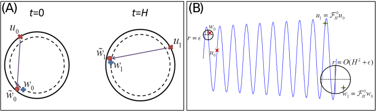
Figure 2: Local and forward alignments. (A) At $t=0$, given two points $u_{0}$ and $v_{0}$, we wish to approximate $w_{0}={\mathcal{S}}_{0}(u_{0};v_{0})$ – a point that has the same slow variables as $u_{0}$ and the same phase as $v_{0}$. At $t=H$, we approximate the point $w_{1}={\mathcal{F}}_{H}w_{0}$ (B) At $t=0$, a small ${\mathcal{O}}(\epsilon)$ of $\tilde{w}_{0}$ yields at $t=H$ a larger ${\mathcal{O}}(H^{2}+\epsilon)$ error. The center of the circles represent $\tilde{w}_{0}$ and $\tilde{w}_{1}$.

In the problem of forward alignment, if $w_{0}$ is a point with the same slow variable as $u_{0}$ and phase as $v_{0}$, then a forward alignment procedure constructs an order $H^{2}$ approximation of $w_{1}={\mathcal{F}}_{H}w_{0}$, the right end point of a coarse interval. See Figure 2A for a schematic sketch.

Notation 3.4.

We denote such a forward alignment procedure as $\tilde{w}_{1}={\mathcal{S}}_{H}^{\lambda}(u_{1};u_{0},v_{0})$, where $\lambda$ are precomputed parameters to be used in the alignment.

The forward alignment procedure can be trivially accomplished simply by setting $\tilde{w}_{1}$ to $v_{1}{\mathcal{F}}_{H}v_{0}$ or $w_{1}$. However, this would require the additional computation of $v_{1}$ from $v_{0}$, and so this trivial ”fix” has a computational cost of sequentially solving the entire system with the fine integrator. In practice, for the purpose of parallel in time computations, one needs to do so with a computational cost that is lower than running the fine scale solver sequentially. Hence, we need to estimate the solution to the given ODE with the given initial condition $v_{0}$ by certain simple operations performed on the fine scale solutions already computed in parallel. In the following section, we shall describe a forward alignment algorithm for the special case of HiOsc ODEs, in which, for fixed slow variables, the fast phase is periodic. The method applies only a local exploration by means of minimal additional fine scale computation of the solution around $u_{0}$ and $u_{1}$. In particular, its efficiency is independent of $\epsilon$.

To summarize, we present the complete multiscale-parareal algorithm. Recall that $\mathcal{M}_{H}$ is a multiscale method that only approximates the slow variables. For the fast phase, using local and forward alignments, we propagate the needed phase adjustments sequentially along with the parareal correction.

Algorithm 3.5.

Full multiscale-parareal algorithm. 1. Initialization: Construct the zero’th iteration approximation: $$u_{0}^{0}=u_{0}\leavevmode\nobreak\ \leavevmode\nobreak\ {\rm and}\leavevmode\nobreak\ \leavevmode\nobreak\ u_{n}^{0}={\mathcal{M}}_{H}u_{n-1}^{0},\leavevmode\nobreak\ \leavevmode\nobreak\ \leavevmode\nobreak\ n=1,\dots,N.$$ 2. Iterations: $k=1...K$ (a) Parallel fine integrations for $n=k,\dots,N$: $$u_{F,n}^{k-1}:=\mathcal{F}_{H}u_{n-1}^{k-1}.$$ (b) Header: For $n=0,\dots,k-1$, set $u_{n}^{k}=u_{F,n}^{k-1}$. (c) Parareal step: Set the initial reference point $u^{*}=u_{k-1}^{k-1}$ and for $n=k,\dots,N$, i. Locally align the previous $u_{n-1}^{k-1}$ with the current reference point $u^{*}$: $$\tilde{u}_{n-1}^{k-1}={\mathcal{S}}_{0}(u_{n-1}^{k-1};u^{*}).$$ ii. Align forward to the end of the coarse segment: $${\tilde{u}_{F,n}^{k-1}={\mathcal{S}}^{\lambda}_{H}(u_{F,n}^{k-1};u_{n-1}^{k-1},u^{*})}.$$ iii. Corrector: $$u_{n}^{k}={\mathcal{S}}_{0}({\mathcal{M}}_{H}u_{n-1}^{k};\tilde{u}_{F,n}^{k-1})+\tilde{u}_{F,n}^{k-1}-{\mathcal{S}}_{0}({\mathcal{M}}_{H}\tilde{u}_{n-1}^{k-1};\tilde{u}_{F,n}^{k-1}).$$ iv. Update the reference point $u^{*}={u}_{n}^{k}$ and repeat.

Local and forward alignment steps (Step 2(c)i and ii, respectively) create a point $\tilde{u}_{F,n}^{k-1}$ at the end of each coarse segment according to which all points in the current corrector iteration can be aligned. Since the error in each forward alignment is of order $H^{2}$, we find that the overall phase is continuous up to a global ${\mathcal{O}}(H)$ error. We conclude that following phase alignments, the aligned coarse multiscale method provides an globally ${\mathcal{O}}(H)$ approximation of both slow and fast variables, i.e., it approximates the solution in the sup norm.

Example 6.2 demonstrates the effectiveness of the method in a more complicated expanding spiral with a slowly changing frequency. Before describing numerical methods for local and forward alignments of HiOsc ODEs, we address the convergence of the algorithm.

3.3 Convergence of Algorithm 3.5

Convergence of Algorithm 3.5 in the state variable is obtained in two steps. First, following Section 3.1 and Theorem 3.3, all slow variables converge to their values obtained by the fine scale integrators,

$$\sup_{n=0,\dots,N}|\xi(u_{n}^{k})-\xi(u(nH))|\leq C(H^{k}+E_{f}),$$

where $C$ is a constant that is independent of $\epsilon$. In particular, if $E_{f}={\mathcal{O}}(\epsilon)$, then, following ${\mathcal{O}}(\log(\epsilon))$ iterations, the error in the slow variables is of order $\epsilon$. As a result, after a few (typically one or two) iterations, the assumptions underlying forward alignment, that the error in the slow variables is of order $\epsilon$ holds (more precisely, $\xi(u_{0})-\xi(v_{0})={\mathcal{O}}(\epsilon)$). We may thus think of the adopted multiscale combined with the local/forward alignment algorithm as a coarse integrator with first order accuracy for all state variables. Hence, the conventional parareal proof of convergence described in Section 1.2 holds. More precisely, suppose that, following the phase alignment, the set $\{w_{0},\dots,w_{N}\}$ is computed and updated in every iteration. The following estimates hold for $j=0,\dots,N$,

$$\left|\xi(w_{j})-\xi(u(jH))\right| ={\mathcal{O}}(E_{m}),$$

$$\left|\phi(w_{j})-\phi(u(jH))\right| ={\mathcal{O}}(H),$$

$$\left|w_{j}-u(jH)\right| ={\mathcal{O}}(H)+{\mathcal{O}}(E_{m}),$$

where $E_{m}$ is the error of the aligned multiscale method in approximating the slow variables.

Assume further the stability properties for the fine and aligned-multiscale coarse propagators (1.6). Therefore, after one parareal iteration,

$$\sup_{n=0,\dots,N}\left|u_{n}^{1}-u(nH)\right|\leq C(\epsilon^{-1}E_{m}+E_{f}).$$

After $k$ iterations, and assuming a first order multiscale coarse integrator, $E_{m}={\mathcal{O}}(H)$,

$$\sup_{n=0,\dots,N}\left|\xi(u_{n}^{k})-\xi(u(nH))\right|\leq C(H^{k}+E_{f}),$$

and

$$\sup_{n=0,\dots,N}\left|u_{n}^{k}-u(nH)\right|\leq C(\epsilon^{-1}H^{k}+E_{f}).$$

The accuracy of slow variables is improved to by a factor of $H$ per parallel iteration (compare with the diverging factor of $(\epsilon^{-1}H)^{k}$ in (1.12)).

Remark 3.6.

In [47], Legoll et al propose a multiscale parareal algorithm for stiff ODEs in which the fast dynamics is dissipative, i.e., trajectories quickly converge to a lower dimensional manifolds. Unlike the HiOsc case, a naive application of the parareal methodology to stiff dissipative systems converges. However, it is not very efficient and suffers from similar difficulties as discussed earlier. To circumvent these difficulties, Legoll et al [47] suggest a correction step that allows a consistent approximation of the fast-slow dynamics with parareal. This work assumes that the system is split into slow and fast variables, or alternatively, that a change of variables that splits the system into such coordinates is given explicitly. Essentially, the idea of [47] is to set the fast component of the multiscale solver with that obtained from the fine one. This step may be viewed as a simple alignment method. Indeed, if the $(\xi,\phi)$ coordinates are know, then the same approach can also be applied to the HiOsc case. In contrast, the method presented in the following section is seamless in the sense that it does not require knowing the slow nor the fast variables.

4 Phase alignment strategies

In this section, we describe a numerical method for both local and forward alignments as defined in the previous section for the special case of HiOsc ODEs in which, for fixed slow variables $\xi$, the dynamics of the fast phase $\phi$ is periodic.

In the Algorithm 3.5, $v_{0}$ and $u_{0}$ will correspond to $u^{k}_{n}$ and $u^{k-1}_{n}$, the solutions computed at the current and the previous iterations, respectively. The assumption is that $v_{0}$ is the more accurate approximation of the solution at the time $t=nH$, particularly in the phase variable. The goal is that from the available information, $u_{0}$, $v_{0}$, and $u_{1}:=\mathcal{F}_{H}u_{0}$, we estimate $v_{1}:=\mathcal{F}_{H}v_{0}$ at $t=(n+1)H$ in order to make correction in the phase of $u_{1}$. We also emphasize that in the subsequent time steps, $\mathcal{F}_{H}u_{0}$ is always available because of the prior parallel fine integrations. Now $w_{0}$, as defined in Section 3.2, is a point on the same slow coordinates as $u_{0}$ but has the same phase as $v_{0}$. Consequently $w_{1}:=\mathcal{F}_{H}w_{0}$ is a good estimate of $v_{1}$. In this section, we propose a strategy that move $u_{0}$ to $w_{0}$, and $u_{1}$ to a state that is within $\mathcal{O}(\epsilon)$ to $w_{1}$, without computing $\mathcal{F}_{H}w_{0}$ or $\mathcal{F}_{H}v_{0}$. Our goal is to describe a method that finds a point $\tilde{w}_{0}$ such that $|w_{0}-\tilde{w}_{0}|={\mathcal{O}}(\epsilon)$ (local alignment) and a second point $\tilde{w}_{1}$ such that $|w_{1}-\tilde{w}_{1}|={\mathcal{O}}(H^{2}+\epsilon)$ (forward alignment).

In addition to Assumption 2.2, we assume the following,

Assumption 4.1.

The fast variable $\phi\in\mathbb{R}$ and $g_{0}(\xi,\phi)$ is 1-periodic in $\phi$.

For fixed $\xi$, the time derivative of $\phi$ may depend on the slow variables, i.e., the periodicity in time of $g_{0}(\xi,\phi(t))$ is of order $\epsilon$ and depends on $\xi$. Accordingly, it is denoted $\epsilon\tau(\xi)$, where $\tau$ is a smooth, slow function. Note that this does not mean that the oscillation in the original state variables are linear because the transformation $\Psi$ is in general nonlinear.

4.1 At time $t$ move $u_{0}$ closer to $w_{0}$

Assuming that $\xi(u_{0})-\xi(v_{0})={\mathcal{O}}(\epsilon)$, we may use $v_{0}$ instead of $w_{0}$, which is not known. Denote

$$J(t;u_{0},v_{0})=\left|{\mathcal{F}}_{t}u_{0}-v_{0}\right|^{2}.$$

We look for the local minima of $J(t;u_{0},v_{0})$ closest to $t=0$ (by the periodicity assumption, such local minima exist)

$$0=J^{\prime}(t;u_{0},v_{0})(t)=2\left({\mathcal{F}}_{t}u_{0}-v_{0}\right)\cdot\frac{d}{dt}\left({\mathcal{F}}_{t}u_{0}-v_{0}\right)=2\left({\mathcal{F}}_{t}u_{0}-v_{0}\right)\cdot\left(\frac{\partial\Psi^{-1}}{\partial\xi}\dot{\xi}+\frac{\partial\Psi^{-1}}{\partial\phi}\dot{\phi}\right).$$

To leading order in $\epsilon$, we have

$$({\mathcal{F}}_{t}u_{0}-v_{0})\cdot(\partial\Psi^{-1}/\partial\phi)={\mathcal{O}}(\epsilon).$$ (4.1)

In other words, the phase of ${\mathcal{F}}_{t}u_{0}$ is close to that of $v_{0}$, $\phi({\mathcal{F}}_{t}u_{0})=\psi_{0}+{\mathcal{O}}(\epsilon)$ and therefore also to the phase of $w_{0}$. We denote the “first” two local minima

$$-\epsilon\tau_{0}+{\mathcal{O}}(\epsilon^{2})<t_{0}^{-}<0<t_{0}^{+}<\epsilon\tau_{0}+{\mathcal{O}}(\epsilon^{2}),$$

where $\tau_{0}=\tau(\xi_{0})$. Consider

$$\tilde{w}_{0}^{\pm}={\mathcal{F}}_{t_{0}^{\pm}}u_{0},$$

and the convex combination using these points,

$$\tilde{w}_{0}={\mathcal{S}}u_{0}=\lambda_{+}\tilde{w}_{0}^{+}+\lambda_{-}\tilde{w}_{0}^{-},$$

with weights $\lambda=(\lambda_{+},\lambda_{-})$ independent of $\epsilon$. Thus, equation (4.1) implies that, for any linear combination such that $\lambda_{+}+\lambda_{-}=1$, $|\tilde{w}_{0}-v_{0}|=\mathcal{O}(\epsilon)$, i.e., $\tilde{w}_{0}$ defined above is a valid choice in the local alignment procedure. We define

Local alignment: $${\mathcal{S}}_{0}(u_{0};v_{0})=\lambda_{+}{\mathcal{F}}_{t_{0}^{+}}u_{0}+\lambda_{-}{\mathcal{F}}_{t_{0}^{-}}u_{0}.$$

In the numerical implementation of the local alignment ${\mathcal{S}}_{0}$, we use a simple algorithm which solves the $l_{2}$ minimization of $J(t)$ with a small ${\mathcal{O}}(\epsilon)$ step size and adaptively increasing the search domain until an appropriate minimum is found. Denoting the time where the minimum is attained by $t^{*}$, we improve the accuracy by a quadratic interpolation through the neighboring points of $t^{*}$. This algorithm achieves ${\mathcal{O}}(\epsilon)$ accuracy with an efficiency that is independent of $\epsilon$. See Appendix A for details and [51] for further references on other efficient minimization techniques.

4.2 At time $t+H$ move $u_{1}$ closer to $w_{1}$

We would like to do the same at $t=H$, i.e., move $u_{1}={\mathcal{F}}_{H}u_{0}$ to $w_{1}={\mathcal{F}}_{H}w_{0}$. The main difficulty is that we cannot expect that the solution has oscillations of constant periodicities. We denote $\tau_{1}=\tau(\xi_{1})=\tau_{0}+(\xi_{1}-\xi_{0})(\partial\tau/\partial\xi)+{\mathcal{O}}(H^{2})$. In analogy to the procedure at $t=0$, we find the “first” two minimizers of

$$J(t;u_{1},w_{1})=\left|{\mathcal{F}}_{t}u_{1}-w_{1}\right|^{2},$$

such that

$$-\epsilon\tau_{1}+{\mathcal{O}}(\epsilon^{2})<t_{1}^{-}<0<t_{1}^{+}<\epsilon\tau_{1}+{\mathcal{O}}(\epsilon^{2}).$$

Let

$$\tilde{w}_{1}=\lambda_{+}\tilde{w}_{1}^{+}+\lambda_{-}\tilde{w}_{1}^{-},\leavevmode\nobreak\ \textrm{with}\leavevmode\nobreak\ \tilde{w}_{1}^{\pm}={\mathcal{F}}_{t_{1}^{\pm}}u_{1}=w_{1}+{\mathcal{O}}(\epsilon).$$

Then, for any constants $\lambda_{+},\lambda_{-}$ we have that $|w_{1}-\tilde{w}_{1}|={\mathcal{O}}(\epsilon)$. The problem is that we do not know $w_{1}$ and therefore cannot find $t_{1}^{\pm}$. One option is to use $t_{0}^{\pm}$ instead and choose weights $\lambda_{\pm}$ that minimize the error. This requires us to relate the $t_{0}$’s and $t_{1}$’s.

Denote

$$\Psi u_{0}=\left(\xi_{0},\phi_{0}\right),\leavevmode\nobreak\ \leavevmode\nobreak\ \leavevmode\nobreak \leavevmode\nobreak\ \leavevmode\nobreak\ \leavevmode\nobreak\ \Psi u_{1}=\Psi{\mathcal{F}}_{H}u_{0}=\left(\xi_{1},\phi_{1}\right),$$

$$\Psi v_{0}=\left(\eta_{0},\psi_{0}\right),\leavevmode\nobreak\ \leavevmode\nobreak\ \leavevmode\nobreak$$

$$\Psi w_{0}=\left(\xi_{0},\psi_{0}\right),\leavevmode\nobreak\ \leavevmode\nobreak\ \leavevmode\nobreak \leavevmode\nobreak\ \leavevmode\nobreak\ \leavevmode\nobreak\ \Psi w_{1}=\Psi{\mathcal{F}}_{H}w_{0}=\left(\xi_{1},\psi_{1}\right).$$

Without loss of generality, we assume that $\psi_{0}>\phi_{0}$ and $|\psi_{0}-\phi_{0}|<1$. Similarly, assume $\psi_{1}>\phi_{1}$ and $|\psi_{1}-\phi_{1}|<1$. Then, to leading order in $\epsilon$,

$$t_{0}^{+}=(\psi_{0}-\phi_{0})\epsilon\tau_{0},\leavevmode\nobreak\ \leavevmode\nobreak\ \leavevmode\nobreak\ \leavevmode\nobreak \leavevmode\nobreak\ \leavevmode\nobreak\ \leavevmode\nobreak\ \leavevmode\nobreak\ t_{1}^{+}=(\psi_{1}-\phi_{1})\epsilon\tau_{1},$$

$$t_{0}^{-}=-(1-\psi_{0}+\phi_{0})\epsilon\tau_{0},\leavevmode\nobreak\ \leavevmode\nobreak\ \leavevmode\nobreak\ \leavevmode\nobreak \leavevmode\nobreak\ \leavevmode\nobreak\ \leavevmode\nobreak\ \leavevmode\nobreak\ t_{1}^{-}=-(1-\psi_{1}+\phi_{1})\epsilon\tau_{1}.$$

Next, denote the solution of $(\xi,\phi)$ with initial condition $(\xi_{0},\phi_{0})$ as $\xi(t;\xi_{0},\phi_{0})$ and $\phi(t;\xi_{0},\phi_{0})$, i.e., $\left(\xi(t;\xi_{0},\phi_{0}),\phi(t;\xi_{0},\phi_{0})\right)=\Psi{\mathcal{F}}_{t}u_{0}$. Using the averaging principle (2.2), we can write

$$\xi(t;\xi_{0},\phi_{0})=\bar{\xi}(t)+\epsilon\gamma(t/\epsilon,\xi)+{\mathcal{O}}(\epsilon^{2}),$$

where $\bar{\xi}(t)$ is a slow function that does not depend on the phase and $\gamma(s,\xi)$ is independent of $\epsilon$ and is $\tau(\xi)$-periodic in $s$ with zero average, $\int_{0}^{\tau(\xi)}\gamma(s,\xi)ds=0$.

$$\phi(H;\xi_{0},\phi_{0}) =\phi_{0}+\int_{0}^{H}\left[\epsilon^{-1}g_{1}(\xi(t;\xi_{0},\phi_{0}))+g_{2}(\xi(t;\xi_{0},\phi_{0}))\right]dt$$

$$=\phi_{0}+\int_{0}^{H}\left[\epsilon^{-1}g_{1}(\bar{\xi}(t))+g_{2}(\bar{\xi}(t))\right]dt+\int_{0}^{H}g^{\prime}_{1}(\bar{\xi}(t))\gamma(t/\epsilon,\bar{\xi}(t))dt+{\mathcal{O}}(\epsilon)$$

$$=\phi_{0}+F(\xi_{0};\epsilon)+{\mathcal{O}}(\epsilon),$$

for some function $F$ that depends only on $\xi_{0}$ and $\epsilon$, but not on the initial phase $\phi_{0}$. In particular, we note that

$$\phi(w_{1})-\psi_{0}=\phi({\mathcal{F}}_{H}w_{0})-\psi_{0}=\phi(H;\xi_{0},\psi_{0})-\psi_{0}=F(\xi_{0};\epsilon)+{\mathcal{O}}(\epsilon).$$

Similarly,

$$\phi_{1}-\phi_{0}=\phi({\mathcal{F}}_{H}u_{0})-\phi_{0}=\phi(H;\xi_{0},\phi_{0})-\phi_{0}=F(\xi_{0};\epsilon)+{\mathcal{O}}(\epsilon).$$

Hence, $\phi(w_{1})-\psi_{0}=\phi_{1}-\phi_{0}={\mathcal{O}}(\epsilon)$. In other words, starting at $w_{0}$ instead of $u_{0}$ introduces a phase shift that is practically constant. We have then

$$t_{1}^{+} =(\psi_{1}-\phi_{1})\epsilon\tau_{1}=\left(\psi_{0}-\phi_{0}\right)\epsilon\left[\tau_{0}+\frac{\partial\tau}{\partial\xi}\cdot(\xi_{1}-\xi_{0})\right]+{\mathcal{O}}(\epsilon H^{2}+\epsilon^{2})$$

$$=(\psi_{0}-\phi_{0})\epsilon\tau_{0}+(\psi_{0}-\phi_{0})\epsilon\frac{\partial\tau}{\partial\xi}\cdot(\xi_{1}-\xi_{0})+{\mathcal{O}}(\epsilon H^{2}+\epsilon^{2})$$

$$=t_{0}^{+}+Ht_{0}^{+}\Delta+{\mathcal{O}}(\epsilon H^{2}+\epsilon^{2}),$$

where $\Delta=\frac{1}{H\tau_{0}}\frac{\partial\tau}{\partial\xi}\cdot(\xi_{1}-\xi_{0})={\mathcal{O}}(1).$ Similarly,

$$t_{1}^{-}=t_{0}^{-}+Ht_{0}^{-}\Delta+{\mathcal{O}}(\epsilon H^{2}+\epsilon^{2}).$$

Consider

$${\mathcal{F}}_{t^{\pm}_{0}}u_{1}={\mathcal{F}}_{-Ht^{\pm}_{0}\Delta}{\mathcal{F}}_{t_{1}^{\pm}}u_{1}+{\mathcal{O}}(\epsilon H^{2}+\epsilon^{2})={\mathcal{F}}_{-Ht^{\pm}_{0}\Delta}\tilde{w}_{1}^{\pm}+{\mathcal{O}}(\epsilon H^{2}+\epsilon^{2}).$$

Expanding around $\tilde{w}_{1}^{\pm}$

$${\mathcal{F}}_{t^{\pm}_{0}}u_{1}=\tilde{w}_{1}^{\pm}-\frac{H}{\epsilon}\delta t_{0}^{\pm}\Delta+{\mathcal{O}}(H^{2}+\epsilon^{2}),$$

for some vector $\delta\in\mathbb{R}^{d}$ independent of $\epsilon$. Therefore, taking a linear combination $\lambda_{+}+\lambda_{-}=1$ and denoting $\lambda=(\lambda_{+},\lambda_{-})$,

$${\mathcal{S}}_{H}^{\lambda}(u_{1};u_{0},v_{0}) = \lambda_{+}{\mathcal{F}}_{t_{0}^{+}}u_{1}+\lambda_{-}{\mathcal{F}}_{t_{0}^{-}}u_{1}$$

$$= \left(\lambda_{+}\tilde{w}_{1}^{+}+\lambda_{-}\tilde{w}_{1}^{-}\right)+\frac{H}{\epsilon}\delta\left(\lambda_{+}t_{0}^{+}+\lambda_{-}t_{0}^{-}\right)\Delta+{\mathcal{O}}(H^{2}+\epsilon^{2})$$

$$= w_{1}+\frac{H}{\epsilon}\delta\left(\lambda_{+}t_{0}^{+}+\lambda_{-}t_{0}^{-}\right)\Delta+{\mathcal{O}}(H^{2}+\epsilon).$$

Finally we see that with the choice

$$\lambda_{+}=\frac{-t_{0}^{-}}{t_{0}^{+}-t_{0}^{-}}\leavevmode\nobreak\ \leavevmode\nobreak\ ,\leavevmode\nobreak\ \lambda_{-}=\frac{t_{0}^{+}}{t_{0}^{+}-t_{0}^{-}},$$

the first order term cancels. Thus, we obtain a second order accurate forward alignment to $w_{1}$. See Figure 3 for the error of (4.2) for the simple example of the expanding spiral (1.11).

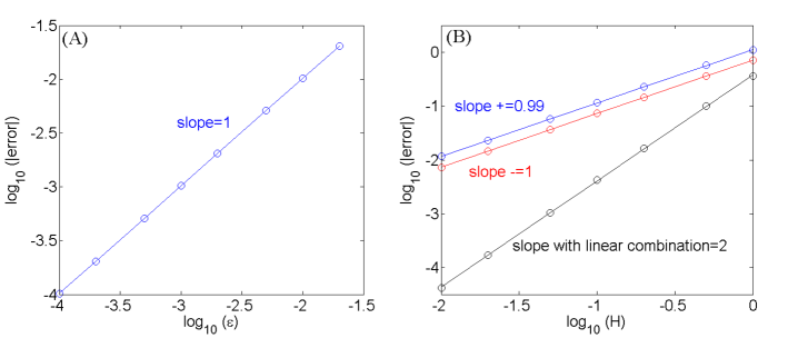
Figure 3: The error in correcting the phase at the end of one coarse segment for the expanding spiral (1.11). (A) In local alignment, the phase at the end of a coarse segment $u_{0}$ is aligned with $v_{0}$ with an ${\mathcal{O}}(\epsilon)$ error. (B) Blue: forward correction with $s_{+}$, red: backward correction with $s_{-}$ and black: a linear combination of shifts using the forward alignment algorithm defined in Section 4. With the proposed linear combination, the error is of order $H^{2}$.

Algorithm 3.5 applies the convex combination (4.2) in forward alignment. Indeed, convergence in the state variable heavily relies on this step because the new point $\tilde{u}_{F,n}^{k-1}$ after the forward alignment is assigned as the reference for local alignment in the next coarse interval. See Step 2(c)iii. We emphasize that taking ${\mathcal{S}}^{\lambda}_{H}$ as (4.2) may shift the slow coordinates of the resulting $u_{1}$ from what was computed by the multiscale coarse integrator and assumed to be accurate. In the next subsection, we propose a more elaborate method to further improve the overall accuracy of the forward alignment step.

4.3 Improving accuracy in forward alignment

Here, the idea is that we identify the convex combination with the point which divides the trajectory of (1.10) originating from ${\mathcal{F}}_{t_{0}^{+}}u_{1}$ and ending close to ${\mathcal{F}}_{t_{0}^{-}}u_{1}$ by a proportion of $\lambda_{-}$ to $\lambda_{+}$. Since there are two orientations of ${\mathcal{F}}_{t}({\mathcal{F}}_{t_{0}^{+}}u_{1})$ defined by forward and backward in time integrations, the modified convex combination will provide us with two points depending on the orientations, and we will choose the one closer to $\mathcal{S}_{H}^{\lambda}u_{1}$.

First, we propose to find the first two local minimizers of

$$J(t;{\mathcal{F}}_{t_{0}^{+}}u_{1},{\mathcal{F}}_{t_{0}^{-}}u_{1})=|\mathcal{F}_{t}({\mathcal{F}}_{t_{0}^{+}}u_{1})-{\mathcal{F}}_{t_{0}^{-}}u_{1}|^{2},$$

such that $-\epsilon\tau_{1}<\Gamma^{-}_{p}<0<\Gamma^{+}_{p}<\epsilon\tau_{1}.$ Denoting

$$t_{0}^{++}=t_{0}^{+}+\lambda_{-}\Gamma^{+}_{p}\textrm{\leavevmode\nobreak\ \leavevmode\nobreak\ and\leavevmode\nobreak\ \leavevmode\nobreak\ }t_{0}^{+-}=t_{0}^{+}+\lambda_{-}\Gamma^{-}_{p},$$ (4.3)

we again find the first local minimizers of

$$J(t;{\mathcal{F}}_{t_{0}^{-}}u_{1},{\mathcal{F}}_{t_{0}^{++}}u_{1}) =|\mathcal{F}_{t}({\mathcal{F}}_{t_{0}^{-}}u_{1})-{\mathcal{F}}_{t_{0}^{++}}u_{1}|^{2},$$ (4.4)

$$J(t;{\mathcal{F}}_{t_{0}^{-}}u_{1},{\mathcal{F}}_{t_{0}^{+-}}u_{1}) =|\mathcal{F}_{t}({\mathcal{F}}_{t_{0}^{-}}u_{1})-{\mathcal{F}}_{t_{0}^{+-}}u_{1}|^{2},$$

such that $-\epsilon\tau_{1}<\Gamma^{-}_{*}<0\textrm{\leavevmode\nobreak\ \leavevmode\nobreak\ and\leavevmode\nobreak\ \leavevmode\nobreak\ }0<\Gamma^{+}_{*}<\epsilon\tau_{1},$ and denote them by

$$t_{0}^{--}=t_{0}^{-}+\Gamma^{-}_{*},\;t_{0}^{-+}=t_{0}^{-}+\Gamma^{+}_{*}.$$ (4.5)

With local minimizers of (4.4), the phases between ${\mathcal{F}}_{t_{0}^{++}}$ and ${\mathcal{F}}_{t_{0}^{--}}$, and between ${\mathcal{F}}_{t_{0}^{+-}}$ and ${\mathcal{F}}_{t_{0}^{-+}}$ are the same. Now, we define the new weights using $t_{0}$’s in (4.3) and (4.5) by

$${\lambda}_{++}=\frac{-t_{0}^{--}}{t_{0}^{++}-t_{0}^{--}},\leavevmode\nobreak\ {\lambda}_{+-}=\frac{-t_{0}^{-+}}{t_{0}^{+-}-t_{0}^{-+}},\leavevmode\nobreak\ {\lambda}_{--}=\frac{t_{0}^{++}}{t_{0}^{++}-t_{0}^{--}},\leavevmode\nobreak\ {\lambda}_{-+}=\frac{t_{0}^{+-}}{t_{0}^{+-}-t_{0}^{-+}}.$$

The convex combination (4.2) is now modified as

$${\mathcal{S}}_{H}^{{\lambda}_{1}}(u_{1};u_{0},v_{0})={\lambda}_{++}{\mathcal{F}}_{t_{0}^{++}}u_{1}+{\lambda}_{--}{\mathcal{F}}_{t_{0}^{--}}u_{1},\;\;{\mathcal{S}}_{H}^{{\lambda}_{2}}(u_{1};u_{0},v_{0})={\lambda}_{+-}{\mathcal{F}}_{t_{0}^{+-}}u_{1}+{\lambda}_{-+}{\mathcal{F}}_{t_{0}^{-+}}u_{1}.$$

Here, we note that

$$\xi({\mathcal{S}}_{H}^{{\lambda}_{1}}(u_{1};u_{0},v_{0}))=\xi(u_{1})+\mathcal{O}(\epsilon),\;\;\xi({\mathcal{S}}_{H}^{{\lambda}_{2}}(u_{1};u_{0},v_{0}))=\xi(u_{1})+\mathcal{O}(\epsilon).$$

In words, the modified convex combinations ${\mathcal{S}}_{H}^{{\lambda}_{1}}(u_{1};u_{0},v_{0})$ and ${\mathcal{S}}_{H}^{{\lambda}_{2}}(u_{1};u_{0},v_{0})$ guarantee the accuracy of order $\epsilon$ in the slow variables of $u_{1}$.

Now, we propose to implement the forward alignment ${\mathcal{S}}_{H}^{\lambda}(u_{1};u_{0},v_{0})$ as follows.

Forward alignment: 1. Set the reference point using (4.2), $\hat{u}:=\lambda_{+}\mathcal{F}_{t_{0}^{+}}u_{1}+\lambda_{-}\mathcal{F}_{t_{0}^{-}}u_{1}$. 2. Compute two modified convex combinations with opposite orientations, $${\lambda}_{++}{{\mathcal{F}}}_{t_{0}^{++}}u_{1}+{\lambda}_{--}{{\mathcal{F}}}_{t_{0}^{--}}u_{1},\;{\lambda}_{+-}{{\mathcal{F}}}_{t_{0}^{+-}}u_{1}+{\lambda}_{-+}{{\mathcal{F}}}_{t_{0}^{-+}}u_{1}.$$ 3. Denote by $\mathcal{S}_{H}^{\lambda}(u_{1};u_{0},v_{0})$ the combination closer to $\hat{u}$.

Remark 4.2.

An unperturbed system of the HiOsc system (1.10), if exists, preserves the slow variables but changes the fast variables. Indeed, by denoting $\mathcal{F}^{0}$ the fine integrator for the unperturbed system, $\xi(\mathcal{F}_{t}^{0}u_{0})=\xi(u_{0})$ for all $t>0$ but $\phi(\mathcal{F}_{t}^{0}u_{0})\neq\phi(u_{0})$ for some $t>0$. If the unperturbed system of (1.10) is explicitly known, one can achieve more accurate local and forward alignments by using $\mathcal{F}^{0}$ in the minimization of $J(t)$. Unfortunately, the unperturbed system is not explicitly known for general systems. Comparison of the parareal solutions using $\mathcal{F}$ with $\mathcal{F}^{0}$ will be presented in Sections 6.1 and 6.6.

5 A multiscale integrator based on Poincaré-map

Even though the goal of the multiscale system is a consistent description of only the slow variables, in practice, obtaining an explicit expression for the slow variables is often difficult or impossible, in particular for high-dimensional systems (see [9] for an example). In [2], a new type of multiscale methods using a Poincaré map technique was introduced. This method only assumes the existence of slow variables but does not use its explicit form. A novel on-the-fly filtering technique achieves high order accuracy. Recall the general two-scale ODE (1.10) with initial condition $u_{0}\in D\subset\mathbb{R}^{d}$:

$$\dot{u}=\epsilon^{-1}f_{1}(u)+f_{0}(u),\,\,\,u(0)=u_{0}.$$ (5.1)

By ignoring the lower order perturbation part of the vector field, an unperturbed dynamical system is defined. The essential part of the Poincaré-map technique is to generate a path whose projection on the slow subspace has the correct slow dynamics. To this end, the scheme solves both the perturbed and the unperturbed systems from the same initial conditions for short time intervals, and compares the resulting trajectories.

The method relies on the following assumptions regarding the HiOsc dynamics

Assumption 5.1.

The dynamics of the unperturbed equation

$$\dot{v}=\epsilon^{-1}f_{1}(v),\,\,\,v(0)=v_{0}.$$ (5.2)

is ergodic with respect to an invariant manifold $\mathcal{M}(v_{0})$.

We denote the solution of (5.2) by $v(t;v_{0})$.

Assumption 5.2.

The invariant manifolds $\mathcal{M}(z)$ is defined by the intersection of the level sets of slow variables $\xi_{1},\xi_{2},\cdots,\xi_{k},$ $k<d$. More precisely, we may identify the invariant manifold of $v$ by level sets of the slow variables for u, $\mathcal{M}(z)=\cap_{j=1}^{k}\{\zeta\in\mathbb{R}^{d}:\xi_{j}(z)=\xi_{j}(\zeta)\}$.

Hence, the solution $u(t)$ defines a foliation of invariant manifolds $\mathcal{M}(t):=\mathcal{M}(u(t))$. Note that our method only assumes the existence of such $\xi$’s but does not require obtaining them.

Suppose we solve the full equation (5.1) and the associated unperturbed version (5.2) with the same initial condition. Then, it is possible to extract the flow of $\mathcal{M}(t)$ from comparison of $u(t)$ and $v(t)$ without explicitly knowing the slow variables. The central idea is to locally create a path $\gamma$ in states space that is transversal to the fast flow. This cut will be defined and approximated by a procedure that realizes a Poincaré return map along it. We shall look for a slow $\gamma(t)$, i.e., require that $|\dot{\gamma}|\leq C$ such that for any slow variable $\xi$, $\xi(\gamma(t))=\xi(u(t))$. In other words, the effective slow path $\gamma(t)$ goes through the same foliation of slow manifolds as the exact solution, $\mathcal{M}(\gamma(t)))=\mathcal{M}(u(t))$. The time derivatives of such effective paths can be obtained by extracting the influence of lower order perturbations in the given oscillatory equation. Approximating the derivative will require solving the HiOsc system for reduced time segments of order $\epsilon$. Since $\gamma$ is slow, it can be approximated using macroscopic integrators with step size $H$ independent of $\epsilon$. As a result, the overall computational complexity of the resulting algorithm is sublinear in $\epsilon^{-1}$.

To be consistent with previous notation, we denote by ${\mathcal{F}}_{t}$ the fine scale approximated propagator for the full equation (1.10), and by ${\mathcal{F}}_{t}^{0}$ the fine scale approximated propagator for the unperturbed equation (5.2) in which the low order perturbation is turned off. In particular, note that under the dynamics of (5.2) all slow variables are constants of motion. Let $\epsilon<\eta<H$. A basic Forward-Euler step, depicted in Figure 4A can be written as

$$u_{n+1}={\mathcal{F}}_{\eta}u_{n}+\frac{H}{\eta}\left({\mathcal{F}}_{\eta}u_{n}-{\mathcal{F}}^{0}_{\eta}u_{n}\right).$$ (5.3)

The values of the effective path $\gamma(t)$ at $t=nH$ is then identified with $u_{n}$, $n=0,1,\cdots,N$. High order approximations of $\gamma(t)$ may be obtained by combining several steps and using high-order extrapolation. The name ”Poincaré technique” alludes to the fact that $\gamma(t)$ is transversal to the solution curves of the unperturbed equation. Thus, the full solution induces a Poincaré return map, which is used to approximate $\gamma(t)$. See [2] for details.

The bottleneck in the efficiency of the new algorithm is a consequence of small-amplitude, high-frequency oscillations in $\xi(u(t))$. The accuracy can be improved by sampling the derivatives of a locally smooth average of $\xi$, $\bar{\xi}$ instead of the weakly oscillating $\xi$. Since we assume no explicit knowledge about the slow variables, $\bar{\xi}$ must be computed intrinsically. In [2], a filtering technique is proposed for the simple case in which the invariant manifold of the unperturbed equation is diffeomorphic to a circle, i.e., the unperturbed dynamics is periodic. More precisely, we propose to replace (1.10) by the filtered equation

$$\dot{\bar{u}}=\epsilon^{-1}f_{1}(\bar{u})+K(t/\eta)f_{0}(\bar{u},t,\epsilon^{-1}t),\,\,\,\,t^{*}\leq t\leq t^{*}+\eta,$$ (5.4)

where the filter $K_{\eta}$ is $C^{q}([0,\eta])$ and satisfies the moment condition of the form

$$\int_{0}^{\eta}K_{\eta}(\eta-s)s^{j}ds=\int_{0}^{\eta}s^{j}ds,j=0,1,2,\cdots,p.$$

The accuracy of (5.4) was demonstrated and analyzed in [2].

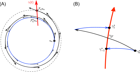
Figure 4: The Poincaré map-type technique approximated all slow variables but does not require knowing their explicit formulas. (A) A forward-Euler type construction. (B) The symmetric Poincaré method is first order, but symmetric with respect to the Poincaré return points.

5.1 Symmetric Poincaré methods

The simple Forward-Euler step (5.3) can be applied in simple situations in which the frequency of the fast oscillation is not a slow variable itself (i.e., $g_{1}$ in (2.1) is not a function of $\xi$) [2]. This restriction can be lifted by generating interpolation points $\gamma^{*}_{k}$ symmetrically described as follows. Our idea it to generate and choose interpolation points $\gamma^{*}$ so that in the state space, $(2\eta)^{-1}\left(\gamma_{1}^{*}-\gamma_{-1}^{*}\right)$ approximates implicitly the derivative of $\bar{\xi}(t)$ but results in small derivative of $\phi(t)$, more precisely, of order $\eta^{2}$. The method, originally proposed and analyzed in [43], can be described as

$$u_{n+1}=\gamma_{-1}^{*}+\frac{H}{2\eta}\left(\gamma_{1}^{*}-\gamma_{-1}^{*}\right),$$ (5.5)

where

$$\gamma_{-1}^{*}={\mathcal{F}}^{0}_{\eta}u_{n},\;\;\gamma_{1}^{*}={\mathcal{F}}^{0}_{-\eta}{\mathcal{F}}_{2\eta}u_{n}.$$

Convergence of the method is proved in Appendix B. See also [43] for different types of Poincaré methods. The method (5.5) defines a propagator, denoted ${\mathcal{M}}_{H}$,

$${\mathcal{M}}_{H}=\left(1-\frac{H}{2\eta}\right){\mathcal{F}}^{0}_{\eta}+\frac{H}{2\eta}{\mathcal{F}}^{0}_{-\eta}{\mathcal{F}}_{2\eta}.$$

The efficiency of the combined parareal with multiscale Poincaré method can be evaluated by counting the number of fine steps in each parareal iteration. An effective time segment $\tau$ is denoted the computational cost of a single parareal iteration equivalent to fine integration of length $\tau$:

$$\tau=H+h_{fine}\eta\left(\frac{4}{h_{Poincare}}+\frac{1}{h_{phase}}\right)\left(1+\frac{T}{H}\right)$$ (5.6)

where $h_{fine}$, $h_{Poincare}$, and $h_{phase}$ are the microscopic step sizes used for fine, Poincaré and phase alignment methods, respectively. Overall, with $K$ iterations, the computational speed-up (assuming maximal parallelization) compared to direct numerical simulation is $T/K\tau$.

6 Numerical examples

6.1 Expanding spiral I

Consider the following nonlinear equation in the complex plane

$$\dot{u}=i\epsilon^{-1}u|u|+u|u|^{-1},$$ (6.1)

with the initial value $u(0)=1$. The associated unperturbed equation is known to be

$$\dot{v}=i\epsilon^{-1}v|v|,\;\;v(0)=v_{0}.$$ (6.2)

As in (2.1), the dynamics of $u(t)$ can be analyzed by the corresponding system of slow and fast variables:

$$\begin{cases}\dot{\xi}=1,&\xi(0)=1,\\ \dot{\phi}=\epsilon^{-1}\xi,&\phi(0)=0.\end{cases}$$ (6.3)

We see immediately from Definition 2.1 that $\xi$ is a slow variable. The difficulty in the phase alignment lies in the singular term in the RHS of $\dot{\phi}$. Note that (6.3) is never used in our algorithm as $\xi$ in (6.3) is only used to show the convergence in the slow variables.

In this example, we use Algorithm 3.5, ODE45 as a fine integrator and the Poincaré 2nd order multiscale method as a coarse integrator (the Midpoint rule macro-solver and ODE45 micro-solver with z-shape construction of $\gamma$) to compute the solution. In each micro-simulation, we solve the filtered equation

$$\dot{u}_{n}(t)=i\epsilon^{-1}u_{n}(t)|u_{n}(t)|+K_{\eta}(t-t_{n})u_{n}(t)|u_{n}(t)|^{-1},\,\,\,t_{n}\leq t\leq t_{n}+\eta,$$ (6.4)

with a $C^{4}$ kernel with $p=1$ supported on $[0,\eta]$ is used. The parameters are specified in Table 2 where $\eta_{Poincare}$ and $h_{Poincare}$ are parameters for (6.4). The absolute errors in the slow variables and in the state variables as a function of parareal iterations for each different $\epsilon=10^{-3}$ and $10^{-4}$ are shown in Figure 5. In addition, we compare the errors when both local and forward alignments are established using the full system (6.1) and the unperturbed system (6.2). The parareal solutions using (6.1) in phase alignments have an error of $\mathcal{O}(\epsilon)$ in the state variables. On the other hand, the phase alignment using (6.2) shows an error in the state variables comparable to that in the slow variables. Indeed, knowing the unperturbed equation (6.2) is an advantage. In applications, obtaining an explicit expression for the unperturbed equation may not be possible, particularly for nonlinear systems.

Table 2: Parareal parameters in Example 6.1.

$T$	$H$	$h_{fine}$	$\eta_{Poincare}$	$h_{Poincare}$	RelTol, AbsTol (ODE45 parameters)
2	1/10	$\epsilon/200$	7$\epsilon$	$\epsilon/10$	$10^{-13}$, $10^{-11}$

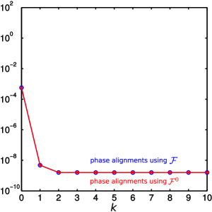
(a) $\epsilon=10^{-3}$

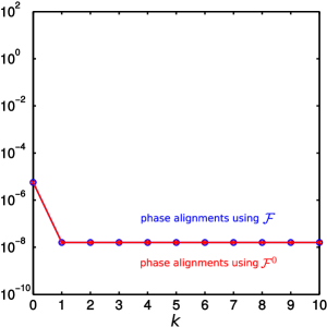
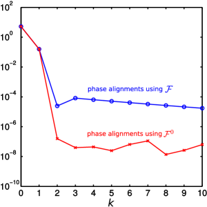
(b) $\epsilon=10^{-4}$

Figure 5: Expanding spiral I, Example 6.1. (Left) Plot of $||\xi(\cdot)-\xi\circ u^{k}(\cdot)||_{L^{\infty}([0,T])}$ as a function of iteration and (Right) the absolute error in the state variables as a function of iteration.

6.2 Expanding spiral with slowly varying fast oscillations

Consider the following HiOsc example

$$\dot{x}=-2\pi\epsilon^{-1}[1+(1-az_{1})z_{2}]y+bx$$ (6.5)

$$\dot{y}=2\pi\epsilon^{-1}[1+(1-az_{1})z_{2}]x+by$$

$$\dot{z}_{1}=1$$

$$\dot{z}_{2}=-az_{2}$$

where $a,b>0$ are constants. Initial conditions are $(x,y,z_{1},z_{2})(0)=(1,0,0,1)$. The solution of (6.5) is $x(t)=e^{bt}\cos\left[2\pi\epsilon^{-1}(1+e^{-at})t\right]$, $y(t)=e^{bt}\sin\left[2\pi\epsilon^{-1}(1+e^{-at})t\right]$, $z_{1}(t)=t$, and $z_{2}(t)=e^{-at}$.

Hence $I=x^{2}+y^{2}$, $z_{1}$ and $z_{2}$ are three slow variables while $(x,y)$ is a linear oscillator with expanding amplitude $\sqrt{I}$ and a slowly changing period $\epsilon/(1+e^{-at})$. The example falls under the general category of HiOsc systems in which the dynamics of the fast phase slowly evolves according to the slow variables. The main difference between this example and Example 6.1 is that the derivative of slow variables is not a constant. As a result, the local ${\mathcal{O}}(H^{2})$ error introduced by the 1st order coarse multiscale integrator is realized.

The system (6.5) is integrated using the full multiscale Poincaré-parareal method, applying the corrected phase shift described in Section 4 to ensure convergence in the state variable. We stress that the numerical approximation is obtained without using our knowledge that the system can be decomposed into the three slow variables $I$, $z_{1}$ and $z_{2}$ and a fast phase-like variable $\phi=\arctan(y/x)$. This decomposition and the exact solution are only used in order to explain the fast-slow structure in the dynamics and for demonstrating the rate of convergence of different variables.

Figure 7A shows the error in the slow variables as a function of iteration. After a single iteration the error in the slow variables drops below $\epsilon$, which is the theoretical limit possible with multiscale methods on their own. Figure 7B shows the absolute error in the state variable of the entire trajectory. Initially, the absolute error is large. This is because the inaccurate slow variables create a jump in the phase between coarse time segments. However, after two iterations, the phase shift becomes accurate and the method converges to the exact solution. Parameters are detailed in Table 4.

Table 3: Parareal parameters in Example 6.2.

$\epsilon$	$T$	$H$	$h_{fine}$	$\eta_{Poincare}$	$h_{Poincare}$	RelTol, AbsTol(ODE45 parameters)
$10^{-3}$	2	0.1	$\epsilon/200$	7$\epsilon$	$\epsilon/10$	$10^{-13}$, $10^{-11}$

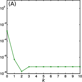
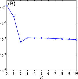
Figure 6: Expanding spiral with $a=0.2$, $b=0.1$, Example 6.2. (A) The error in the slow variables, $\underset{i=1,2,3}{\max}||\xi_{i}(\cdot)-\xi_{i}\circ u^{k}(\cdot)||_{L^{\infty}([0,T])}$, as a function of iteration. (B) The absolute error in the state variables as a function of iteration.

6.3 Stellar orbits in a galaxy

The following system is taken from the theory of stellar orbits in a galaxy [39, 40]:

$$\begin{cases}\ddot{r}_{1}+a^{2}r_{1}=\epsilon r_{2}^{2},\\ \ddot{r}_{2}+b^{2}r_{2}=2\epsilon r_{1}r_{2}.\end{cases}$$

Following a change of variables $\mathbf{x}=[x_{1},v_{1},x_{2},v_{2}]^{T}=[r_{1},\frac{d}{d\tau}r_{1}/a,r_{2},\frac{d}{d\tau}r_{2}/b]^{T}$ and after a rescaling of time, $t=\epsilon\tau$, the system can be written in the following form

$$\dot{x}_{1}=\epsilon^{-1}av_{1}$$ (6.6)

$$\dot{v}_{1}=-\epsilon^{-1}ax_{1}+x^{2}_{2}/a$$

$$\dot{x}_{2}=\epsilon^{-1}v_{2}$$

$$\dot{v}_{2}=-\epsilon^{-1}x_{2}+2x_{1}x_{2}/b.$$

Initial conditions are $(x_{1},v_{1},x_{2},v_{2})(0)=(1,0,1,0)$. Resonance of oscillatory modes take effect in the lower order term when $a=2$ and $b=1$. Using the algorithm proposed in [5], three independent slow variables are identified as

$$\xi_{1}=x_{1}^{2}+v_{1}^{2},\,\,\,\,\,\,\,\,\xi_{2}=x_{2}^{2}+v_{2}^{2},\,\,\,\,\,\,\,\,\xi_{3}=x_{1}x_{2}^{2}+2v_{1}x_{2}v_{2}-x_{1}v_{2}^{2}.$$ (6.7)

The example falls under the category of HiOsc systems in which two stiff harmonic oscillators are coupled. The local ${\mathcal{O}}(H^{2})$ error introduced by the 1st order coarse multiscale integrator is realized.

The system (6.6) is integrated using Algorithm 3.5, applying the global alignment algorithm described in Section 4 to ensure convergence in the state variable. The Poincaré method is used as a coarse solver, using the trajectory of (6.6) as the flow ${\mathcal{F}}$ and the one of (6.6) without a lower order perturbation as the flow ${\mathcal{F}}^{0}$. We stress that the numerical approximation is obtained without using our knowledge that the system can be decomposed into the three slow variables $\xi_{1}$, $\xi_{2}$ and $\xi_{3}$ and a fast phase-like variable $\phi$. This decomposition are only used in order to explain the fast-slow structure in the dynamics.

Figure 7 shows the absolute error in the state variable of the entire trajectory. Initially, the absolute error is large because the inaccurate slow variables create a jump in the phase between coarse time segments. However, after four iterations the error in the state variable drops below $\epsilon$, which is the theoretical limit possible with multiscale methods on their own. Parameters are detailed in Table 4. The fine integrator is ODE45 method, and the coarse integrator is the Poincaré 2nd order multiscale method. A $C^{3}$ kernel with $p=1$ is used for the filtered equation.

Table 4: Parareal parameters in Example 6.3.

$\epsilon$	$T$	$H$	$h_{fine}$	$\eta_{Poincare}$	$h_{Poincare}$	RelTol, AbsTol(ODE45 parameters)
$10^{-4}$	14	0.5	$\epsilon/100$	20$\epsilon$	$\epsilon/10$	$10^{-13}$, $10^{-11}$

Figure 7: Stellar orbits in a galaxy, Example 6.3. The absolute error in the state variables as a function of iteration is depicted.

6.4 Non-linear oscillators

Consider the following example of a Voltera-Lotka oscillator with slowly varying frequency and amplitude

$$\dot{x}=\epsilon^{-1}x(1-zy)$$

$$\dot{y}=\epsilon^{-1}zy(x-1)$$

$$\dot{z}=0.2x$$

Initial conditions are $(x,y,z)(0)=(1,2.9,1)$. For fixed $z$, $(x,y)$ is a Voltera-Lotka oscillator whose period is of order $\epsilon$. The period and amplitude of $(x,y)$ depend on a parameter $z$, which is given by the time integral of $x$. As a result, $z$ is a slow variable. It is easily verified that the first integral of the oscillator is also slow,

$$I=x-\log(x)+y-\log(y)/z$$

Again, we stress that the slow variables are only used in order to demonstrate the results of the method. They are not used in the numerical approximation. In addition, Figure 8A shows the level set of the slow variable, $\left\{u\in\mathbb{R}^{3}:I(u)=I(x(t_{n}),y(t_{n}),z(t_{n}))\right\}$, projected onto x-y plane. In contrast to the previous examples, the level set of the slow variable $I$ is not a circle. As a result, $J(t)$ may have several local minima and we need to find the first local minima which is close to the global minimum of $J$ within a few periods. Parameters are given in Table 5. The fine integrator is ODE45 method, and the coarse integrator is the Poincaré 2nd order multiscale method. A $C^{3}$ kernel with $p=1$ is used for the filtered equation.

Table 5: Parareal parameters in Example 6.4.

$\epsilon$	$T$	$H$	$h_{fine}$	$\eta_{Poincare}$	$h_{Poincare}$	RelTol, AbsTol(ODE45 parameters)
$10^{-3}$	10	1/2	$\epsilon/200$	30$\epsilon$	$\epsilon/10$	$10^{-13}$, $10^{-10}$

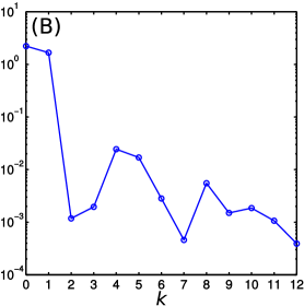
Figure 8: A Lotka-Voltera oscillator with slowly varying frequency and amplitude, Example 6.4. (A) The level sets of the slow variable $I$ projected onto $x$-$y$ plane. (B) The absolute error in the state variables as a function of iteration.

6.5 Passage through resonance

One of the fundamental assumptions underling multiscale approaches such as Poincaré and other methods is a spectral gap in the spectrum of the Jacobian of the equations of motion. When this assumption fails, for example due to a temporary passage through resonance, the assumption 3.1 may not hold close the resonance and typical multiscale methods fail. However, the applicability of the multiscale algorithms can be extended by the parareal approach described above, i.e., by resolving all scales of the dynamics - both the slow and the fast.

We consider the following example.

$$\dot{x}=-2\pi\epsilon^{-1}f(z)y+0.5\sin(z)x$$

$$\dot{y}=2\pi\epsilon^{-1}f(z)x$$

$$\dot{z}=1$$

where

$$f(z)=\tanh\left(50(z-4.5)\right).$$

Initial conditions are $(1,0,0)$. In words, $f(z)$ changes smoothly from -1 to 1, vanishing at $z=4.5$. Hence, the frequency of oscillation undergoes fast oscillations with varying frequency, except close to $t=4.5$. At this time, $f(z)$ vanishes and the system is no longer highly oscillatory. More precisely, trajectories go through a transition layer. Its width in this example is of order $\epsilon$. The two slow variables are $I=x^{2}+y^{2}$ and $z$.

Figure 9A shows the values of the state variables with $\epsilon=10^{-4}$. Due to the resonance, the Poincaré method fails to capture the correct evolution of the slow variables when crossing the singular point $t=4.5$. However, combining with parareal, the fine solution of parareal integrates the equation across the resonance and allows the multiscale method to proceed beyond the singularity. In Figure 9B, the absolute error in the state variable does not decrease with iterations because the accuracy of phase alignment relies on the scale separation which does not exists near $t=4.5$. We show, however, that the convergence in the state variable can be achieved with a slight modification of Algorithm 3.5. Figure 9C is obtained by skipping phase alignments, Step 2(c)i and ii, and replacing Step (c)iii with the naive correction (1.2) in the interval near $t=4.5$.

Remark 6.1.

We note that this example goes beyond the scope for which convergence is proven in Section 4. Indeed, the purpose of the example is to demonstrate that the applicability of the multiscale-parareal coupling using alignments may be wider than proven here.

Table 6: Parareal parameters in Example 6.5.

$\epsilon$	$T$	$H$	$h_{fine}$	$\eta_{Poincare}$	$h_{Poincare}$	RelTol, AbsTol(ODE45 parameters)
$10^{-4}$	7	1/4	$\epsilon/200$	15$\epsilon$	$\epsilon/10$	$10^{-13}$, $10^{-11}$

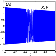
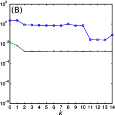
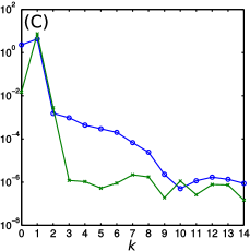
Figure 9: Passage through resonance, Example 6.5. (A) The solution of $x(t)$ and $y(t)$ with $t\in[4,5]$ and $\epsilon=10^{-4}$. The frequency function vanishes at $t=4.5$ and solutions lose their highly oscillatory nature. (B) The absolute errors of both state (circles) and slow (crosses) variables as a function of iterations with phase alignment at all the time. (C) The absolute errors with phase alignment turned off near $t=4.5$. Convergence in the state variable is achieved.

6.6 The Fermi-Pasta-Ulam (FPU) problem

We consider a chain of $2k$ springs on a line, connected with alternating soft nonlinear and stiff linear springs with both ends fixed. This problem has been used as a benchmark for testing the long-time performance of geometric integrators [31]. See also [14, 15, 30] and references therein for related recent work. The model is derived from the following Hamiltonian:

$$H(p,q)=\frac{1}{2}\overset{2k}{\underset{i=1}{\sum}}p_{i}^{2}+\frac{1}{4}\epsilon^{-2}\overset{k}{\underset{i=1}{\sum}}(q_{2i}-q_{2i-1})^{2}+\overset{k}{\underset{i=1}{\sum}}(q_{2i+1}-q_{2i})^{4}.$$

Using the change of variables given in [5], the equations of motion for the system can be written as

$$\begin{cases}\dot{y}_{i}=u_{i},\\ \dot{x}_{i}=\epsilon^{-1}v_{i},\\ \dot{u}_{i}=-(y_{i}-\epsilon x_{i}-y_{i-1}-\epsilon x_{i-1})^{3}+(y_{i+1}-\epsilon x_{i+1}-y_{i}-\epsilon x_{i})^{3},\\ \dot{v}_{i}=-\epsilon^{-1}x_{i}+(y_{i}-\epsilon x_{i}-y_{i-1}-\epsilon x_{i-1})^{3}+(y_{i+1}-\epsilon x_{i+1}-y_{i}-\epsilon x_{i})^{3}.\end{cases}$$ (6.8)

Since the ends are fixed, $y_{0}=x_{0}=y_{k+1}=x_{k+1}=0$.

In this section, we endeavor solving (6.8) in the $\mathcal{O}(\epsilon^{-1})$ time scale using the proposed methods. The aim is to expose the limit of the various different algorithmic components of the proposed methods. Clearly, the time scale in which we compute the solutions of (6.8) is out of the scope of the analysis that we presented earlier.

System (6.8) is solved in $\mathbb{R}^{8}$ with $k=2$, and it admits seven slow variables — they are the total energies of the stiff springs, $I_{i}=x_{i}^{2}+v_{i}^{2}$ for $i=1,2$, the relative phases between the stiff springs, $\phi=x_{1}x_{2}+v_{1}v_{2}$, and all the degrees of freedom which are related to the soft springs: $y_{i}$ and $u_{i}$, $i=1,2$. The nontrivial energy transfer and the relative phase take place in the very long $\epsilon^{-1}$ time scale.

In Figure 10A, we present the maximum errors in the state variable in a long time interval $[0,T]=[0,\epsilon^{-1}/2]$, with $\epsilon=10^{-3}$. The system (6.8) is integrated using Algorithm 3.5, applying the global alignment algorithm described in Section 4 to achieve convergence in the state variable. The results are computed with the initial conditions $y_{1}=x_{1}=y_{2}=x_{2}=1$, $(u_{1},v_{1},u_{2},v_{2})=(0,1.2,1,0)$ and with the parameters given in Table 7. The Verlet method was used as the fine integrator and the Poincaré 2nd order method (Verlet macro-solver and ODE45 micro-solver) as the multiscale integrator. We further point out that the errors will decrease as $\epsilon$ becomes smaller.

In Figure 10B, we present the maximum errors computed using the same set of conditions and parameters, except that the phase alignments are computed by the numerical solutions of the modified equation:

$$\begin{cases}\dot{y}_{i}=0\cdot u_{i},\\ \dot{x}_{i}=\epsilon^{-1}v_{i},\\ \dot{u}_{i}=0\cdot\left\{-(y_{i}-\epsilon x_{i}-y_{i-1}-\epsilon x_{i-1})^{3}+(y_{i+1}-\epsilon x_{i+1}-y_{i}-\epsilon x_{i})^{3}\right\},\\ \dot{v}_{i}=-\epsilon^{-1}x_{i}+0\cdot\left\{(y_{i}-\epsilon x_{i}-y_{i-1}-\epsilon x_{i-1})^{3}+(y_{i+1}-\epsilon x_{i+1}-y_{i}-\epsilon x_{i})^{3}\right\},\end{cases}$$ (6.9)

with $y_{0}=x_{0}=y_{k+1}=x_{k+1}=0$. This is a slightly more general type of “unperturbed” equations as those defined in Section 5. This approach may be thought of as phase alignments with some slow variables constrained. A detailed discussion about such topic is out of the scope of this paper, and shall be addressed in a future work.

Remark 6.2.

We observe that in this study, phase alignments by solutions of (6.9) yield significantly superior results. Indeed, our experience indicated that for the problems that can be solved by the Poincaré method described in Section 5, it is generally better to use the so-called “unperturbed” equations for phase alignments, as the slow variables are constrained and would not deteriorate the performance of the phase alignment steps. However, we chose to present a more general setup in this paper, avoiding any specific choice of coarse/multiscale integrators in describing the algorithms.

Table 7: Parareal parameters in Example 6.6.

$\epsilon$	$T$	$H$	$h_{fine}$	$\eta_{Poincare}$	$h_{Poincare}$	RelTol, AbsTol(ODE45 parameters)
$10^{-3}$	$\epsilon^{-1}/2$	$1/4$	$\epsilon/20$	$10\epsilon$	$\epsilon/20$	$10^{-12}$, $10^{-10}$

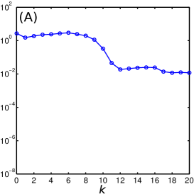
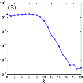
Figure 10: The Fermi-Pasta-Ulam problem, Example 6.6. The absolute error in the state variables as a function of iteration is depicted. (A) Phase alignments with the full system (6.8). (B) Phase alignments with the unperturbed equation explained in the paragraph.

7 Summary

The paper describes two approaches to incorporate multiscale integrators as coarse integrators in parareal methods. The first, presented in Section 3.1, approximates all the slow variables. However, the numerical approximation of the state variables $u_{n}^{k}$ does not converge to the true solution $u(nH)$. This parareal-multiscale combination has several advantages compared to other multiscale schemes.

• It offers increased stability and is less sensitive to the choice of parameters. Intuitively, the parareal iterations can ”fix” errors incurred by the inexact multiscale scheme.

• It offers increased accuracy. In fact, the accuracy of slow variables may be smaller than ${\mathcal{O}}(\epsilon)$, which is a theoretical limit for Poincaré and other multiscale methods that are based on averaging or homogenization principles.

• It may be applied for systems with moderate scale separation. Most multiscale methods are more efficient than conventional, non-multiscale schemes if the separation in scale is large enough, i.e., if $\epsilon$ is sufficiently small. However, they typically become less efficient or unstable at intermediate values of $\epsilon$.

• The method may be used in situations in which the dynamics looses its multiscale structure in a short transition layer, for example, due to passage through resonance, see Example 6.5.

The second approach, presented in Section 3.2, computes convergent approximation to all state variables in the system. This algorithm requires the phase alignment procedure, described in Section 4 in addition to the steps needed in our first algorithm. We prove that the accuracy of the scheme in the sup norm after $K$ iterations is of order $\epsilon^{-1}H^{K}+E_{f}$, where $H$ is the a coarse step size. In particular, the number of iterations to achieve a given error tolerance is logarithmic in $\epsilon^{-1}$.

The computational cost of the method can be divided into two contributions. The first is the cost of the fine integrator invoked at each parareal iteration. With $K$ iterations its contribution to the overall cost is proportional to $KH\epsilon^{-1}$. The second contribution comes from the overhead of coarse multiscale integrators and phase alignment. While this contribution is independent of $\epsilon$, it grows linearly with the number of coarse step sizes, $H^{-1}$. Hence, there is a trade off in choosing $H$. With a large scale separation $\epsilon\ll 1$, the first contribution dominates and, assuming maximal parallelization is available, it is advantageous to use a relatively small $H$, even if the multiscale method allows larger steps. The two contributions balance if one takes $H=\sqrt{\epsilon}$, which implies a computational cost of order $K\epsilon^{-1/2}$. In contrast, parallel methods using conventional integrators will require at least $\mathcal{O}(\epsilon^{-1})$ steps.

The multiscale-parareal coupling strategy using alignments is not limited to the proposed particular implementation involving a single-frequency fast variable. In the multi-frequency case, different alignment algorithms may be possible. For example, if the slow-fast system is given explicitly, one could simply set the fast variable in the coarse integrator to coincide with the fine one.

Acknowlegments

Tsai’s research is supported by a Simons Foundation Fellowship, NSF grants DMS-1217203, and DMS-1318975.

Appendix A Appendix: Adaptive search algorithm

We explain our implementation for the local alignment ${\mathcal{S}}_{0}$. This algorithm adaptively searches local minima of the functional $J(t)$ by adjusting the step size and the computational interval. The first part of the algorithm numerically solves the $l_{2}$ minimization problem of $J(t)$ using quadratic interpolation. The second part computes a convex combination for the local alignment ${\mathcal{S}}_{0}(u_{0};v_{0})$.

For simplicity, we assume that the fine solver applies a numerical method with step size $h={\mathcal{O}}(\epsilon)$. Also, let $\eta=\eta_{phase}>0$ denote a parameter that is larger than at least one period. It is assumed that $\eta$ is of order $\epsilon$, but the size of $\eta$ is not explicitly known. Our algorithm adaptively finds the size of $\eta$ and locally integrates the HiOsc ODE in short time segments of length $[-\eta,\eta]$. Thus, the computational cost of each alignment procedure is independent of $\epsilon$.

Recall that at $t=0$, given two points $u_{0}$ and $v_{0}$ such that $|\xi(u_{0})-\xi(v_{0})|={\mathcal{O}}(\epsilon)$, local alignment approximates a new point $w_{0}$ such that $\xi(w_{0})=\xi(u_{0})$ and $\phi(w_{0})=\phi(v_{0})$. In addition, first forward and backward alignment times $t_{0}^{\pm}$ are sought, in which $|{\mathcal{F}}_{t_{0}^{\pm}}u_{0}-v_{0}|$ are local minima.

In the following, denote by $[x]$ the integer value of $x$.

Algorithm A.1.

Local alignment ${\mathcal{S}}_{0}(u_{0};v_{0})$

1. Adaptive search for first two local minima of $J(t)$ associated with positive(+) and negative(-) orientations.

   1. Set $\eta=\epsilon$, $h=\epsilon/100$, $Tol=\infty$, $u_{prev}=\infty$, and $I_{\pm}=\{\}.$

   2. While $Tol>\epsilon/100$ or $I_{\pm}\neq\{\}$

      1. Forward/Backward local integration: Compute $u_{0,i}=\mathcal{F}_{ih}u_{0}$, $i\in\{0,\dots,[\pm\eta/h]\}.$

      2. Compute the local minimum of $J(i)=|u_{0,i}-v_{0}|^{2},$ $i\in\{0,\dots,[\pm\eta/h]\}$.
         Denote it $I_{\pm}=(i_{1\pm},i_{2\pm},\cdots,i_{r\pm})$.

      3. If $I_{\pm}\neq\{\}$, set $Tol=|u_{prev}-u_{0,i_{1\pm}}|$, $u_{prev}=u_{0,i_{1\pm}},$ and $h=h/2$.
         Else, set $\eta=2\eta$ and $h=\epsilon/100$.

      End while.

   3. Quadratic interpolation: For each of the first two indices $i_{1\pm}$, improve the minimization of $J$ using a quadratic interpolation. Let $p_{\pm}(t)$ denote the polynomial such that

      $$p_{\pm}(i_{1\pm}+j)=u_{0,i_{1\pm}+j},\quad j=-1,0,1.$$

      Denote by $t_{0}^{\pm}$ the minimum of $|p_{\pm}(t)-v_{0}|$.

2. Let

   $$\lambda_{+}=\frac{t_{0}^{-}}{t_{0}^{+}+t_{0}^{-}}\leavevmode\nobreak\ \leavevmode\nobreak\ ,\leavevmode\nobreak\ \lambda_{-}=\frac{t_{0}^{+}}{t_{0}^{+}+t_{0}^{-}},$$

   and define

   $${\mathcal{S}}_{0}(u_{0};v_{0})=\lambda_{+}{\mathcal{F}}_{t_{0}^{+}}u_{0}+\lambda_{-}{\mathcal{F}}_{t_{0}^{-}}u_{0}.$$ (A.1)

In (A.1), we implement the fine integrator ${\mathcal{F}}$ with step size $h$ determined in step 1(b). If $t_{0}^{\pm}/h$ is not integer, then ${\mathcal{F}}$ is to be evaluated using quadratic interpolation.

Appendix B Appendix: Convergence of the symmetric Poincaré method

To prove convergence of the symmetric Poincaré method algorithm described in Section 5.1, we use a diffeomorphism $\Psi:u\rightarrow(\xi(u),\phi(u))$ given in (2.1),

$$\begin{cases}\dot{\xi}=g_{0}(\xi,\phi),&\xi(0)=\xi(u_{0}),\\ \dot{\phi}=\epsilon^{-1}g_{1}(\xi)+g_{2}(\xi,\phi),&\phi(0)=\phi(u_{0}),\end{cases}$$ (B.1)

where $g_{0}(\xi,\phi)$ and $g_{2}(\xi,\phi)$ are 1-periodic in $\phi$. We stress that the variables $(\xi,\phi)$ are only used in the analysis but not in the numerical algorithm. In Section 2, the dynamics of the slow variables can be approximated by an averaged equation of (2.2),

$$\dot{\bar{\xi}}=F(\bar{\xi}),\leavevmode\nobreak\ \leavevmode\nobreak\ \leavevmode\nobreak\ F({\bar{\xi}})=\int g_{0}(\xi,\phi)d\phi_{\xi},$$ (B.2)

$$\bar{\xi}(0)=\xi(u_{0}).$$

Recall that the construction given in Section 5.1,

$$u_{n+1}=\gamma_{-1}^{*}+\frac{H}{2\eta}\left(\gamma_{1}^{*}-\gamma_{-1}^{*}\right).$$

To simplify the calculation, we generate $\gamma^{*}$ using the symmetric shape ($z$-shape) which is centered at $\gamma^{*}_{0}$. See Figure 4. The formulas for $\gamma^{*}_{-1}$, $\gamma^{*}_{0}$ and $\gamma^{*}_{1}$ are thus of the form

$$\gamma_{-1}^{*}={\mathcal{F}}^{0}_{\eta}{\mathcal{F}}_{-\eta}u_{n},\leavevmode\nobreak\ \leavevmode\nobreak\ \gamma_{0}^{*}=u_{n},\leavevmode\nobreak\ \leavevmode\nobreak\ \gamma_{1}^{*}={\mathcal{F}}^{0}_{-\eta}{\mathcal{F}}_{\eta}u_{n}.$$

We then prove the following theorem.

Theorem B.1.

The Poincaré force estimator defined by

$$\mathcal{P}=\frac{1}{2\eta}\left({\mathcal{F}}^{0}_{-\eta}{\mathcal{F}}_{\eta}-{\mathcal{F}}^{0}_{\eta}{\mathcal{F}}_{-\eta}\right)$$

satisfies the following estimates in the $(\xi,\phi)$ coordinate:

$$\xi(\mathcal{P}u_{n})=\frac{d}{dt}\bar{\xi}(t_{n})+E_{F},\leavevmode\nobreak\ \leavevmode\nobreak\ \leavevmode\nobreak\ \left|\phi(\mathcal{P}u_{n})\right|=\mathcal{O}\left(\frac{\eta^{2}}{\epsilon}\right)$$ (B.3)

where $E_{F}$ denotes the error of the filtered equation in approximating an averaged equation.

Proof.

Consider the unperturbed system associated with (B.1),

$$\begin{cases}\dot{\xi}=0,&\xi(0)=\xi_{0},\\ \dot{\phi}=\frac{1}{\epsilon}g_{1}(\xi),&\phi(0)=\phi_{0}.\end{cases}$$ (B.4)

When $\mathcal{F}$ is corresponding to the filtered equation (5.4), it is proved in [2] that $\mathcal{F}_{\pm\eta}u_{n}$ is essentially close to averaged $\bar{\xi}(t_{n}\pm\eta)$, respectively. We denote by $(\xi^{+},\phi^{+})$ the slow-fast coordinate of the point $\gamma_{1}^{*}$, i.e., $(\xi^{+},\phi^{+})=(\xi(\gamma^{*}_{1}),\phi(\gamma^{*}_{1}))$. Similarly, $(\xi^{-},\phi^{-})=(\xi(\gamma^{*}_{-1}),\phi(\gamma^{*}_{-1}))$. Then $\xi^{+}$ and $\phi^{+}$ satisfy

$$\begin{cases}\xi^{+}=\xi_{0}+\int_{0}^{\eta}F(\bar{\xi}^{F}(t))dt,\\ \phi^{+}=\phi_{0}+\int_{0}^{\eta}\frac{1}{\epsilon}g_{1}(\bar{\xi}^{F}(t))dt+\int_{0}^{\eta}G(\bar{\xi}^{F}(t))dt-\frac{\eta}{\epsilon}g_{1}(\xi^{+}),\end{cases}$$

where $\bar{\xi}^{F}(t)$ corresponds to the solution of (B.2) forward in time and $G$ is the averaged $g_{2}(\xi,\phi)$ due to the filtered equation. On the other hand, for $\gamma_{-1}^{*}$,

$$\begin{cases}\xi^{-}=\xi_{0}-\int_{0}^{\eta}F(\bar{\xi}^{B}(t))dt,\\ \phi^{-}=\phi_{0}-\int_{0}^{\eta}\frac{1}{\epsilon}g_{1}(\bar{\xi}^{B}(t))dt-\int_{0}^{\eta}G(\bar{\xi}^{B}(t))dt+\frac{\eta}{\epsilon}g_{1}(\xi^{-}),\end{cases}$$

where $\bar{\xi}^{B}(t)$ corresponds to the backward in time solution of (B.2).

For the slow variables, evaluating the force by $\gamma^{*}_{1}-\gamma^{*}_{-1}$ yields

$$\xi^{+}-\xi^{-}=\int_{0}^{\eta}F(\bar{\xi}^{F}(t))dt+\int_{0}^{\eta}F(\bar{\xi}^{B}(t))dt$$

which approximates the evolution of $\bar{\xi}$ over the interval $[-\eta,\eta]$. For the fast variable,

$$\phi^{+}-\phi^{-} = \underset{I_{1}}{\underbrace{\int_{0}^{\eta}\frac{1}{\epsilon}g_{1}(\bar{\xi}^{F}(t))dt-\frac{\eta}{\epsilon}g_{1}(\xi^{+})+\int_{0}^{\eta}\frac{1}{\epsilon}g_{1}(\bar{\xi}^{B}(t))dt-\frac{\eta}{\epsilon}g_{1}(\xi^{-})}}$$

$$+\underset{I_{2}}{\underbrace{\int_{0}^{\eta}G(\bar{\xi}^{F}(t))dt-\int_{0}^{\eta}G(\bar{\xi}^{B}(t))dt}}.$$

By considering $\bar{\xi}^{F}(t)=\xi_{0}+\int_{0}^{t}F(\bar{\xi}^{F})ds$ and $\bar{\xi}^{B}(t)=\xi_{0}-\int_{0}^{t}F(\bar{\xi}^{B})ds$, we can compute the Taylor series to estimate $\epsilon I_{1}$, developed at $\xi_{0}$.

$$\epsilon I_{1} = \left\{\int_{0}^{\eta}g_{1}\left(\xi_{0}+\int_{0}^{t}F(\bar{\xi}^{F}(s))ds\right)dt-\eta g_{1}\left(\xi_{0}+\int_{0}^{\eta}F(\bar{\xi}^{F}(t))dt\right)\right\}$$

$$+\left\{\int_{0}^{\eta}g_{1}\left(\xi_{0}-\int_{0}^{t}F(\bar{\xi}^{B}(s))ds\right)dt-\eta g_{1}\left(\xi_{0}-\int_{0}^{\eta}F(\bar{\xi}^{B}(t))dt\right)\right\}$$

$$= \left\{\int_{0}^{\eta}\left(\int_{0}^{t}\nabla{g}_{1}(\xi_{0})^{T}F(\bar{\xi}^{F}(s))ds\right)dt-\eta\int_{0}^{\eta}\nabla{g}_{1}(\xi_{0})^{T}F(\bar{\xi}^{F}(t))dt\right\}$$

$$-\left\{\int_{0}^{\eta}\left(\int_{0}^{t}\nabla{g}_{1}(\xi_{0})^{T}F(\bar{\xi}^{B}(s))ds\right)dt-\eta\int_{0}^{\eta}\nabla{g}_{1}(\xi_{0})^{T}F(\bar{\xi}^{B}(t))dt\right\}+\mathcal{O}(\eta^{3}).$$

Here, the terms $\eta g_{1}\left({\xi}_{0}\right)$ canceled. Due to the symmetric structure, expanding both $\bar{\xi}^{F}(s)$ and $\bar{\xi}^{B}(s)$ about $s=0$ using Taylor series, all $\mathcal{O}(\eta^{2})$ terms vanish and we have

$$\epsilon I_{1}=\mathcal{O}(\eta^{3}).$$

Similarly, one can show that

$$I_{2}=\mathcal{O}(\eta^{2}).$$

Therefore, there exist nonnegative constants $C_{1}$ and $C_{2}$ such that

$$\left|\phi(\gamma_{1}^{*})-\phi(\gamma_{-1}^{*})\right|=|\phi^{+}-\phi^{-}|\leq C_{1}\frac{\eta^{3}}{\epsilon}+C_{2}\eta^{2}.$$ (B.5)

This completes the proof. ∎

It is important to use an appropriate sequence of interpolating points in the state space, $\gamma_{k}^{*},$ as it directly impacts on the accuracy of Poincaré method. With a parameter $\eta=C\epsilon$, (B.3) shows that the force estimator $\mathcal{P}$ generates two interpolating points to estimate the evolution of the slow variables over $2\eta$ with an $\mathcal{O}(\epsilon)$ disagreement in the fast variable. This results in stable and accurate approximations. However, we remark that the force estimation using the algorithm (5.3) sometimes introduces an $\mathcal{O}(1)$ difference in the fast variable and thus shifts the slow variables.

References

- [1] A. Abdulle, W. E, B. Engquist, and E. Vanden-Eijnden. The heterogeneous multiscale method. Acta Numerica, 21:1–87, 2012.
- [2] G. Ariel, B. Engquist, S. Kim, Y. Lee, and R. Tsai. A multiscale method for highly oscillatory dynamical systems using a Poincaré map type technique. J. Sci. Comput., 54(2-3):247–268, 2013.
- [3] G. Ariel, B. Engquist, S. J. Kim, and R. Tsai. Iterated averaging of three-scale oscillatory systems. Commun. Math. Sci., 12(5):791–824, 2014.
- [4] G. Ariel, B. Engquist, H.-O. Kreiss, and R. Tsai. Multiscale computations for highly oscillatory problems. In Multiscale modeling and simulation in science, volume 66 of Lect. Notes Comput. Sci. Eng., pages 237–287. Springer, Berlin, 2009.
- [5] G. Ariel, B. Engquist, and R. Tsai. A multiscale method for highly oscillatory ordinary differential equations with resonance. Math. Comp., 78:929–956, 2009.
- [6] G. Ariel, B. Engquist, and R. Tsai. Numerical multiscale methods for coupled oscillators. Multi. Mod. Simul., 7:1387–1404, 2009.
- [7] G. Ariel, B. Engquist, and R. Tsai. A reversible multiscale integration method. Comm. Math. Sci., 7:595–610, 2009.
- [8] G. Ariel, B. Engquist, and R. Tsai. Oscillatory systems with three separated time scales – analysis and computation. In Numerical analysis of multi scale computations, volume 82 of Lect. Notes Comput. Sci. Eng., pages 23–45. Springer, Berlin, 2011.
- [9] Z. Artstein, C. W. Gear, I. G. Kevrekidis, M. Slemrod, and E. S. Titi. Analysis and computation of a discrete KdV-Burgers type equation with fast dispersion and slow diffusion. SIAM Journal on Numerical Analysis, 49(5):2124–2143, 2011.
- [10] Z. Artstein, I. G. Kevrekidis, M. Slemrod, and E. S. Titi. Slow observables of singularly perturbed differential equations. Nonlinearity, 20(11):2463–2481, 2007.
- [11] Z. Artstein, J. Linshiz, and E. S. Titi. Young measure approach to computing slowly advancing fast oscillations. Multiscale Model. Simul., 6(4):1085–1097, 2007.
- [12] C. Audouze, M. Massot, and S. Volz. Symplectic multi-time step parareal algorithms applied to molecular dynamics. 2009.
- [13] G. Bal and Q. Wu. Symplectic parareal. In Domain decomposition methods in science and engineering XVII, volume 60 of Lect. Notes Comput. Sci. Eng., pages 401–408. Springer, Berlin, 2008.
- [14] D. Bambusi and A. Ponno. On metastability in FPU. Comm. Math. Phys., 264(2):539–561, 2006.
- [15] D. Bambusi and A. Ponno. Resonance, metastability and blow up in FPU. In The Fermi-Pasta-Ulam problem, volume 728 of Lecture Notes in Phys., pages 191–205. Springer, Berlin, 2008.
- [16] A. Blouza, L. Boudin, and S.M. Kaber. Parallel in time algorithms with reduction methods for solving chemical kinetics. Comm. in Applied Math. and Comput. Sci., 5:241–263, 2010.
- [17] F. Casas and A. Iserles. Explicit magnus expansions for nonlinear equations. Journal of Physics A: Mathematical and General, 39(19):5445–5461, 2006.
- [18] M. Condon. Efficient computation of delay differential equations with highly oscillatory terms. ESAIM: Mathematical Modelling and Numerical Analysis, 46(06):1407–1420, 2012.
- [19] M. Condon, A. Deano, and A. Iserles. On second-order differential equations with highly oscillatory forcing terms. Proceedings of the Royal Society A: Mathematical, Physical and Engineering Science, 2010.
- [20] X. Dai, C. Le Bris, F. Legoll, and Y. Maday. Symmetric parareal algorithms for hamiltonian systems. ESAIM: Mathematical Modelling and Numerical Analysis, 47:717–742, 2013.
- [21] W. E and B. Engquist. The heterogeneous multiscale methods. Commun. Math. Sci., 1(1):87–132, 2003.
- [22] W. E, B. Engquist, X. Li, W. Ren, and E. Vanden-Eijnden. Heterogeneous multiscale methods: A review. Comm. Comput. Phys., 2:367–450, 2007.
- [23] S. Engblom. Parallel in time simulation of multiscale stochastic chemical kinetics. SIAM Multiscale Model. Simul., 8:46–68, 2009.
- [24] B. Engquist, A. Fokas, E. Hairer, and A. Iserles. Highly Oscillatory Problems. Cambridge University Press, New York, NY, USA, 1st edition, 2009.
- [25] B. Engquist and Y.-H. Tsai. Heterogeneous multiscale methods for stiff ordinary differential equations. Math. Comp., 74(252):1707–1742, 2005.
- [26] I. Fatkullin and E. Vanden-Eijnden. A computational strategy for multiscale chaotic systems with applications to Lorenz 96 model. J. Comp. Phys., 200:605–638, 2004.
- [27] M.J. Gander and E. Hairer. Analysis for parapreal algorithms applied to hamiltonian differential equations. J. Comp. Appl. Math., 259:2–13, 2014.
- [28] C. W. Gear and I. G. Kevrekidis. Constraint-defined manifolds: A legacy code approach to low-dimensional computation. J. Sci. Comput., 25(1-2):17–28, 2005.
- [29] D. Givon, R. Kupferman, and A.M. Stuart. Extracting macroscopic dynamics: Model problems and algorithms. Nonlinearity, 17:R55–R127, 2004.
- [30] E. Hairer and C. Lubich. On the energy distribution in Fermi-Pasta-Ulam lattices. Preprint, 2010.
- [31] E. Hairer, C. Lubich, and G. Wanner. Geometric Numerical Integration, volume 31 of Springer Series in Computational Mathematics. Springer-Verlag, Berlin, 2002. Structure-preserving algorithms for ordinary differential equations.
- [32] T. Haut and B. Wingate. An asymptotic parallel-in-time method for highly oscillatory pdes. arXiv, page 1303.6615, 2013.
- [33] L. He. The reduced basis technique as a coarse solver for parareal in time simulations. J. Comput. Math, 28:676–692, 2010.
- [34] A. Iserles. Think globally, act locally: Solving highly-oscillatory ordinary differential equations. Applied Numerical Mathematics, 43(1-2):145–160, 2002.
- [35] A. Iserles. On the numerical quadrature of highly-oscillating integrals i: Fourier transforms. IMA Journal of Numerical Analysis, 24(3):365–391, 2004.
- [36] A. Iserles and S. P. Norsett. On quadrature methods for highly oscillatory integrals and their implementation. BIT Numerical Mathematics, 44(4):755–772, 2004.
- [37] A. Iserles and S. P. Norsett. Efficient quadrature of highly oscillatory integrals using derivatives. Proceedings of the Royal Society A: Mathematical, Physical and Engineering Science, 461(2057):1383–1399, 2005.
- [38] H. Jiménez-Pérez and J. Laskar. A time-parallel algorithm for almost integrable hamiltonian systems. 2011.
- [39] J. Kevorkian and J. D. Cole. Perturbation Methods in Applied Mathematics, volume 34 of Applied Mathematical Sciences. Springer-Verlag, New York, Heidelberg, Berlin, 1980.
- [40] J. Kevorkian and J. D. Cole. Multiple Scale and Singular Perturbation Methods, volume 114 of Applied Mathematical Sciences. Springer-Verlag, New York, Berlin, Heidelberg, 1996.
- [41] I. G. Kevrekidis and G. Samaey. Equation-free multiscale computation: Algorithms and applications. Annu. Rev. Phys. Chem., 60:321–344, 2009.
- [42] M. Khanamiryan. Quadrature methods for highly oscillatory linear and nonlinear systems of ordinary differential equations: part i. BIT Numerical Mathematics, 48(4):743–761, 2008.
- [43] S. J. Kim. Numerical methods for highly oscillatory dynamical systems using multiscale structure. PhD thesis, University of Texas at Austin, 2013.
- [44] H.-O. Kreiss. Problems with different time scales for ordinary differential equations. SIAM J. Numer. Anal., 16(6):980–998, 1979.
- [45] H.-O. Kreiss. Problems with different time scales. In Acta numerica, 1992, pages 101–139. Cambridge Univ. Press, 1992.
- [46] H.-O. Kreiss and J. Lorenz. Manifolds of slow solutions for highly oscillatory problems. Indiana Univ. Math. J., 42(4):1169–1191, 1993.
- [47] F. Legoll, T. Lelievre, and G. Samaey. A micro-macro parareal algorithm: application to singularly perturbed ordinary differential equations. SIAM J. Sci. Comput., 2013.
- [48] D. Levin. Fast integration of rapidly oscillatory functions. Journal of Computational and Applied Mathematics, 67(1):95–101, 1996.
- [49] J.-L. Lions, Y. Maday, and G. Turinici. A ”parareal” in time discretization of pde’s. Comptes Rendus de l’Academie des Sciences, 332:661–668, 2001.
- [50] Y. Maday. The parareal in time algorithm. In Substructuring Techniques and Domain Decomposition Methods, volume 44, page 19. Saxe-Coburg Publications, Stirlingshire, UK, 2010.
- [51] J. Nocedal and S. J. Wright. Numerical optimization. Springer Series in Operations Research and Financial Engineering. Springer, New York, second edition, 2006.
- [52] R.L. Petzold, O.J. Laurent, and Y. Jeng. Numerical solution of highly oscillatory ordinary differential equations. Acta Numerica, 6:437–483, 1997.
- [53] J. A. Sanders, F. Verhulst, and J. Murdock. Averaging methods in nonlinear dynamical systems, volume 59 of Applied Mathematical Sciences. Springer, New York, second edition, 2007.
- [54] R. Sharp, Y.-H. Tsai, and B. Engquist. Multiple time scale numerical methods for the inverted pendulum problem. In Multiscale methods in science and engineering, volume 44 of Lect. Notes Comput. Sci. Eng., pages 241–261. Springer, Berlin, 2005.
- [55] M. Tao, H. Owhadi, and J. Marsden. Nonintrusive and structure preserving multiscale integration of stiff odes, sdes, and hamiltonian systems with hidden slow dynamics via flow averaging. Multi. Mod. Simul., 8:1269–1324, 2010.