Periodic interference structures in the time-like proton form factor

Abstract

An intriguing and elusive feature of the time-like hadron form factor is the possible presence of an imaginary part associated to rescattering processes. We find evidence of that in the recent and precise data on the proton time-like form factor measured by the BABAR collaboration. By plotting these data as a function of the 3-momentum of the relative motion of the final proton and antiproton, a systematic sinusoidal modulation is highlighted in the near-threshold region. Our analysis attributes this pattern to rescattering processes at a relative distance of 0.7-1.5 fm between the centers of the forming hadrons. This distance implies a large fraction of inelastic processes in $\bar{p}p$ interactions, and a large imaginary part in the related $e^{+}e^{-}\rightarrow\bar{p}p$ reaction because of unitarity.

Electromagnetic hadron form factors (FFs) are fundamental quantities which describe the internal structure of the hadron (for a recent review see Ref. Pacetti et al. (2015)). FFs enter explicitly in the coupling of a virtual photon with the hadron electromagnetic current, and can be directly compared to hadron models which describe dynamical properties of hadrons. They are experimentally accessible through the knowledge of the differential cross section and the polarization observables.

Traditionally most data on FFs come from electron-proton elastic scattering. It is assumed that the interaction occurs through the exchange of a single virtual photon which carries a four momentum transfer squared $q^{2}$. In this kinematical region (space-like, SL) the virtual photon-proton coupling and the electron-proton scattering cross section are described via two real FFs, electric, $G_{E}$, and magnetic, $G_{M}$.

FFs have been also studied in the time-like (TL) region of momentum transfer squared. They are measured through the reactions

$$e^{+}\ +\ e^{-}\ \to\ \bar{p}\ +p\ ,$$ (1)

$$\bar{p}\ +\ p\ \to\ e^{+}\ +\ e^{-}\ ,$$ (2)

where a hadron pair is formed by or annihilated into a virtual photon. In the following we will refer to the former reaction, when not otherwise specified.

Assuming single photon exchange, the unpolarized cross section contains the squared moduli of two TL FFs (electric and magnetic FF), which are complex-valued functions of $q^{2}$. The imaginary part is expected to be large and information on the relative phase between $G_{E}$ and $G_{M}$ can be extracted from single spin polarization experiments Dubnickova et al. (1996) which are presently out of reach. In this letter evidence for periodic structures in TL FF data is reported and related to their complex nature.

Many models for the hadron coupling to the virtual photon have been developed and applied to the calculation of SL FFs. Some of them may be analytically continued to the TL region. This is the case for approaches based on vector meson dominance Bijker and Iachello (2004); Adamuscin et al. (2005) and dispersion relations Belushkin et al. (2007); Lomon and Pacetti (2012). Constituent quark models in light front dynamics may be applied de Melo et al. (2004), as well as approaches based on AdS/QCD correspondence Brodsky and de Teramond (2008). A phenomenological picture has been recently proposed for an interpretation of FFs in both the SL and TL regions Kuraev et al. (2012).

The individual determination of the electric and magnetic TLFF is obtained in principle, from the angular distribution of reactions (1,2), but until now the luminosity was not sufficient. The various experimental results are therefore compared on the basis of a generalized FFBardin et al. (1994), which is related to the unpolarized cross section by: $\sigma$:

$$|F_{p}|^{2}=\displaystyle\frac{3\beta q^{2}\sigma}{2\pi\alpha^{2}\left(2+\displaystyle\frac{1}{\tau}\right)},$$ (3)

where $\alpha=e^{2}/(4\pi)$, $\beta=\sqrt{1-1/\tau}$, $~{}\tau={q^{2}}/(4M^{2})$, and $M$ is the proton mass.

Even in these simplified terms, it has long been difficult to analyze with precision the behavior of the data over a broad kinematic range because of the uncertainties and of the matching of data from different experiments which covered limited $q^{2}$ regions. The recent data by the BABAR collaboration Lees et al. (2013a, b) cover with reasonable continuity a region ranging from slightly over the $\bar{p}p$ threshold to $q^{2}$ $\approx$ 36 GeV². In particular about 30 data points have been extracted in the region $q^{2}$ $<$ 10 GeV², with a relative error lower than 10 %. These features allow for a refined analysis of the systematic behavior of the TLFF, where large-scale and small-scale (in $q^{2}$ sense) properties of the data distribution may be scrutinized.

From now on, we use the expression ”near-threshold region” to indicate a $q^{2}$-range extending from the threshold of the $\bar{p}p$ channel up to $q^{2}$ $\approx$ 9 GeV² (with the convention $c=\hbar=1$). In this kinematic region, two different scales participate: the total energy of the colliding $e^{+}e^{-}$ pair is $>2M\approx 1.9$ GeV, while the kinetic energy of the created $\bar{p}p$ pair is relatively small. Therefore one may expect to observe complex effects where a highly relativistic formation picture expressed in terms of quarks and gluons coexists with non relativistic interactions of two slow hadrons leaving the formation zone.

Proton-antiproton interactions in the near-threshold region have been studied in experiments at LEAR (see Zenoni et al. (1999a, b) and references therein for previous data) and more recently at AD Bianconi et al. (2011). These measurements could not separate spin channels and, as in the case of the single effective FF of Eq. (3), these data have been mostly analyzed in terms of a single effective scattering amplitude, as if proton and antiproton were scalar particles.

We define ”large inelasticity” when, writing the amplitude as a sum of partial waves, at least half of the incoming flux is absorbed for all the partial waves of angular momentum $L$ satisfying $L\leq Rp$, $R\simeq 1$ fm. The unitarity limit is reached when there is total absorption for these waves. For the inelastic cross section $\bar{p}+p\to X\neq\bar{p}+p$ ”large inelasticity” occurs in all the kinematical range of interest here, with the possible exception of the region $p$ $<$ 50 MeV Bianconi et al. (2000); Bruckner et al. (1990). For $p\gg$ 100 MeV the inelastic cross section of $\simeq$ 40 mb is close to the black disk limit $\approx$ 50 mb.

As a consequence, unitarity leads to a large imaginary part in the amplitude of $\bar{p}+p\rightarrow$ exclusive final states, including (2). Near the threshold this is rigorously stated by Watson’s final state theorem Watson (1952) applied to reaction (1). More in general the presence of a large transition amplitude $\bar{p}+p\rightarrow A_{n}$, where $A_{n}$ is an on-shell channel, implies a contribution to the imaginary part of the amplitude of (2) from a Cutkosky cut applied to the intermediate state of the 2-step process $\bar{p}+p\rightarrow A_{n}\rightarrow e^{+}+e^{-}$.

Understanding at which extent phenomenological $\bar{p}p$ interactions could be final state interactions of the reaction (1) and seriously affect its amplitude, is however complicated by an evident ”mismatch” of two known features of these processes:

1) The analysis of annihilation and scattering data has shown that colliding proton and antiproton do not overlap at small kinetic energies. As soon as these particles come close within 1 fm of each other, they either annihilate or scatter in a hard-core way Bianconi et al. (2000); Batty et al. (2001). So the wave function describing a $\bar{p}p$ state presents a ”hole” of size 1 fm. Within a momentum range of 400 MeV over the $\bar{p}p$ threshold, this property is demonstrated by counter-intuitive phenomena as the equality of $\bar{p}p$, $\bar{p}$D, and $\bar{p}^{4}$He annihilation cross sections at small energies Bianconi et al. (2000)), and the suppressed effect of the electric charge in $\bar{p}$-nucleus annihilation with the paradoxical effect of $\bar{n}$ cross sections on heavy nuclei exceeding $\bar{p}$ ones Friedman (2014).

2) In the exclusive reaction (1) quark-counting rules Matveev et al. (1973); Brodsky and Farrar (1973) predict that in the initial stages of the formation process quarks and antiquarks are concentrated in a region of size $1/\sqrt{q^{2}}$, which means at a relative distance of 0.1 fm when $q^{2}\approx$ 4 GeV ². So, in the initial formation stages the hadrons lie at a distance that is not normally tested in phenomenological $\bar{p}p$ interactions, making rescattering effects largely unpredictable.

In order to search for signals of final state effects at small kinetic energies in the data, it is more convenient to introduce variables directly related to the relative motion of the hadron pair. In the following we will use the 3-momentum $p$ of one of the two hadrons in the frame where the other one is at rest:

$$p\ \equiv\ \sqrt{E^{2}-M^{2}},\hskip 8.5359ptE\ \equiv\ q^{2}/(2M)\ -\ M.$$ (4)

The usefulness of this variable presumes that the process can be divided into two stages: formation and rescattering, where the latter involves energies on a smaller scale than the former. This means that the amplitude for the process is the sum of a leading term due to a ”bare formation” process taking place on a time scale $1/\sqrt{q^{2}}$, and a relatively small perturbation associated to rescattering processes taking place on a larger time scale.

A consequence of this assumption is that the measured FFs can be fitted by a function of the form :

$$F(p)\ \equiv\ F_{0}(p)\ +\ F_{osc}(p),$$ (5)

$$|F_{osc}(p)|\ \ll\ |F_{0}(p)|,$$ (6)

$$<F_{osc}(p)>_{\Delta p}\ \rightarrow\ 0\ for\ \Delta p\ \gg\ 1\ \mbox{GeV}^{2},$$ (7)

where:

• $F_{0}(p)$ is the translation in terms of the variable $p$ of a known parametrization that has been adjusted on the data in the full range $4M^{2}<q^{2}\lesssim$ 36 GeV² (see below) ignoring small-scale oscillations. $F_{0}(p)$ is regular and smooth on the GeV/c scale. We name it “regular background fit”.

• $F_{osc}(p)$ reproduces GeV-scale or sub-GeV-scale irregularities in the lower part of the $p$ range. We name it “oscillation fit”. $<F_{osc}(p)>_{\Delta p}$ is the local average of $F_{osc}(p)$ over the momentum range $[p-\Delta p/2,p+\Delta p/2]$.

The data by the BABAR collaboration Lees et al. (2013a, b) are selected for this study, since they are the most precise data in the near-threshold region and they cover with continuity a very large kinematic range. Both properties are necessary for our analysis. The fitting procedure is the one of the Minuit package of root.cern.ch Brun and Rademakers (1997), based on the minimization of $\chi^{2}=\sum_{i}(f(x_{i},p_{i})-y_{i})^{2}/\sigma_{i}^{2}$, where $\sigma_{i}$ is the error on the point of coordinates $(x_{i},y_{i})$ and $f$ is the fitting function depending on the parameters $p_{i}$. The error on $p_{i}$ is the interval where $\chi^{2}/n.d.f.$ increases by one unit ($n.d.f.$ is the number of degrees of freedom: number of points minus number of parameters).

To satisfy Eq. (7) a good choice of the regular background term $F_{0}(p)$ is needed. The generalized FF has been consistently extracted at $e+e^{-}$ colliders and antiproton facilities. It shows a decreasing behavior as function of $q^{2}$, which was generally fitted in the experimental papers before the year 2006 with the function Ambrogiani et al. (1999); Lepage and Brodsky (1979):

$$|F_{scaling}(q^{2})|=\displaystyle\frac{\cal A}{(q^{2})^{2}\log^{2}(q^{2}/\Lambda^{2})}.$$ (8)

A good fit of the data prior to BABAR last results was obtained with ${\cal A}=40$ GeV^-4 and $\Lambda=.45$ GeV².

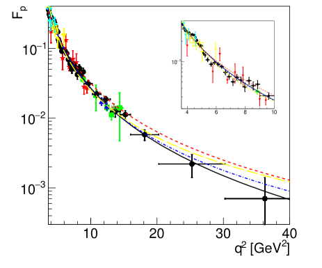
Fig. 1: World data on the TL proton generalized FF as a function of $q^{2}$, together with the calculation from Eq. (8) (blue dash-dotted line), Eq. (9) (red dashed line), Eq. (10) (yellow long-dashed line), and Eq. 12 (black solid line). The world data are from Ref. Lees et al. (2013a, b) (black solid circles), Ref. Ablikim et al. (2005) (red stars), Ref. Ambrogiani et al. (1999) (green squares), Ref. Andreotti et al. (2003) (blue triangles up), Ref. Antonelli et al. (1994) (yellow triangles down ), Ref. Bisello et al. (1983, 1990) (cyan full crosses), Ref. Delcourt et al. (1979) (magenta full diamonds), and Ref. Pedlar et al. (2005)(dark green asterisk). The insert magnifies the near threshold region.

Based on Ref. Shirkov and Solovtsov (1997), in order to avoid ghost poles in $\alpha_{s}$ the following modification was suggested (Kuraev ):

$$|F_{scaling+corr}(q^{2})|\ =\ \displaystyle\frac{\cal A}{(q^{2})^{2}\left[\log^{2}(q^{2}/\Lambda^{2})+\pi^{2}\right]}.$$ (9)

In this case the best fit parameters are ${\cal A}=72$ GeV^-4 and $\Lambda=0.52$ GeV².

In Ref. Brodsky and de Teramond (2008) a form was suggested with two poles of dynamical origin (induced by a dressed electromagnetic current)

$$|F_{T3}(q^{2})|\ =\ \displaystyle\frac{\cal A}{(1-q^{2}/m_{1}^{2})(2-q^{2}/m_{2}^{2})}.$$ (10)

The best fit parameters are ${\cal A}=1.56$, $m_{1}^{2}=1.5$ GeV² and $m_{2}^{2}=0.77$ GeV².

The TLFF data from the BABAR collaboration Lees et al. (2013a, b) were obtained from the reaction

$$e^{+}+e^{-}\ \rightarrow\bar{p}+p\ +\ \gamma,\\$$ (11)

where the photon is preferentially emitted in the entrance channel. These data, extending from the threshold to $q^{2}\approx 36$ GeV², are well reproduced by the function Tomasi-Gustafsson and Rekalo (2001):

$$|F_{BABAR}(q^{2})|\ =\ \frac{\cal A}{(1+q^{2}/m_{a}^{2})\left[1-q^{2}/0.71\right]^{2}},$$

$${\cal A}=7.7~{}\mbox{GeV}^{-4},\ m_{a}^{2}=14.8~{}\mbox{GeV}^{2}.$$ (12)

The world data are shown in Fig. 1 as a function of the transferred momentum $q^{2}$, and compared with the fits from Eqs. (8,9,10,12). The near-threshold region is highlighted in the insert.

In the following, we present results with $F_{0}(p)\ \equiv\ F_{BABAR}[q^{2}(p)].$ This function does not follow the expected asymptotic QCD counting rules, but best reproduces the BABAR data, the slope of which is steeper than $1/(q^{2})^{2}$. It has to be considered as a local approximation of some more complicated function. We have checked that, taking any of the above background possibilities gives consistent results (within the errors) although the fit has a smaller $\chi^{2}$/n.d.f. using $F_{BABAR}$.

In Fig. 2a the BABAR data are plotted as a function of $p$. The result of the fit using Eq. (12) is then subtracted from the data. This difference ${\cal D}$ (i.e., data minus $F_{0}(p)$) is shown in Fig. 2b and exhibits a damped oscillatory behavior, with regularly spaced maxima and minima. Assuming that the first maximum is at $p$ $=$ 0, the distance between this, the 2nd and the 3rd maximum is $\Delta p$ $\approx$ 1.14 GeV. After the 3rd maximum the oscillations of the data are within the error bars.

This behavior is fitted with the 4-parameter function

$$F_{osc}(p)\ \equiv\ A\ \exp(-Bp)\ \cos(Cp\ +\ D).$$ (13)

The values of the parameters are reported in Table 1.

Tab. 1: Fit parameters from Eq. (13).

$A\pm\Delta A$	$B\pm\Delta B$	$C\pm\Delta C$	$D\pm\Delta D$	$\chi^{2}/n.d.f$
	$[GeV]^{-1}$	$[GeV]^{-1}$
$0.05\pm 0.01$	$0.7\pm 0.2$	$5.5\pm 0.2$	$0.03\pm 0.3$	1.2

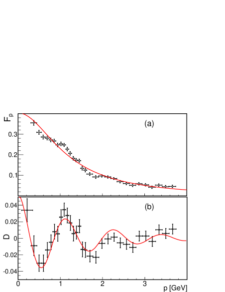
Fig. 2: (a): TL proton generalized FF as a function of $p$ from Ref. Lees et al. (2013a, b); the line is the regular background fit with Eq. (12); (b): data after subtraction of the fit; the line is the fit with Eq. (13).

The relative size of the oscillating term over the regular background is $\sim$ 10 %. The damping range of the oscillations of Fig. 2b is $1/B$ $\approx$ 1.4 GeV. $F_{0}(p)$ decreases by a factor $1/e$ within about 1.5 GeV. The relative magnitude of the oscillations to the regular background term $F_{0}(p)$ does not change much at increasing $p$, although increasing errors make the oscillations undetectable for $p>3$ GeV ($q^{2}>10$ GeV²). At asymptotically large $q^{2}$ values, the Phragmén-Lindelöff theorem Titchmarsh (1939) requires that the imaginary part of TLFFs vanishes, which implies that rescattering disappears. So, although we expect a large-momentum suppression of the relative weight of the rescattering terms, this is not seen in the range $q^{2}<10$ GeV² where error bars allow us to distinguish systematic from statistical oscillations in the data.

The periodicity and the simple shape of the oscillations seem to exclude a random arrangement of maxima and minima of heterogeneous origin. Rather, they indicate a unique interference mechanism behind all the visible modulation. A simple oscillatory behavior in $p$ means that the waves corresponding to the outgoing particles originate from a small number of coherent interfering sources: these waves may share a common initial source but be rescattered along different paths or in different ways so to acquire different phases. We may speak of “alternative rescattering pathways”. These must be in a small number and there must be discontinuity among them, otherwise we would see diffraction patterns instead of interference patterns. For example, in Kuraev et al. (2012) it has been suggested that, during the intermediate stages of $\bar{p}p$ formation, charge and color are distributed in a highly inhomogeneous way, with discontinuity features.

Since we do not know the rescattering mechanism, we cannot identify the sources of rescattered waves, but we may gain some clue on their space distribution. Let $\vec{r}$ be the space variable that is conjugated to $\vec{p}$ via three-dimensional Fourier transform. We may identify $r$ as the distance between the centers of the two forming or formed hadrons, in the frame where one is at rest. Let $M_{0}(r)$ and $M(r)$ be the Fourier transforms of the regular background fit and of the complete fit:

$$F_{0}(p)\equiv\ \int d^{3}\vec{r}\ exp(i\vec{p}\cdot\vec{r})\ M_{0}(r)$$ (14)

$$F(p)=F_{0}(p)+F_{osc}(p)\equiv\int d^{3}\vec{r}\ exp(i\vec{p}\cdot\vec{r})M(r).$$ (15)

$M_{0}(r)$ is shown in Fig. 3, left panel. The most relevant feature is that $M_{0}(r)$ decreases by 7 orders of magnitude for $r$ ranging from 0 and to 2 fm. The decrease is regular and almost constant on a semilog scale. $M_{0}(r)$ is steep near the origin, too. From a mathematical point of view this follows from the fact that at the threshold of the $\bar{p}p$ channel the function $F_{0}(p)$ is a regular, continuous, and rapidly decreasing function of $q^{2}$. It can be interpreted by the fact that both $F_{0}(p)$ and its transform $M_{0}(r)$ are expression of that short distance quark-level dynamics Matveev et al. (1973); Brodsky and Farrar (1973) that permits exclusive $\bar{p}p$ production at the condition that the final quarks and antiquarks are formed within a small region. Near threshold, the size of this region is $\leq 0.1$ fm, much smaller than the standard hadron size.

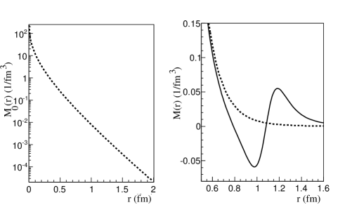
Fig. 3: (Left) $M_{0}(r)$, Eq. (14) . (Right): $M(r)$ (solid line) from Eq. (15), and $M_{0}(r)$ (dashed line) for comparison (linear vertical scale).

In the right panel of Fig. 3 $M(r)$ is superimposed to $M_{0}(r)$. We notice that these two functions do not differ for $r<0.7$ fm, and that the physical reason of the data oscillation must be searched for in processes taking place in the $r$-range 0.7-1.5 fm. This range is important because it includes the distances corresponding to the largest annihilation probability in the phenomenological $\bar{p}p$ interactions in the near-threshold region Bianconi et al. (2000); Batty et al. (2001); Friedman (2014). At a distance of 1 fm, the relevant part of rescattering must involve physical or almost physical hadrons that annihilate into groups of 2-10 mesons. As discussed above, this means a large contribution to the imaginary part of the amplitude for $\gamma^{*}\rightarrow\bar{p}p$ from the Cutkosky cuts applied to all the 2-step processes like $\gamma^{*}\rightarrow n\pi\rightarrow\bar{p}p$, where $n\pi$ is a state composed by $n$ on-shell pions (or other mesons).

Rescattering with a phase shift between alternative channels may take place via formation of $s$-channel poles, or via $t-$channel photon/meson exchanges. Both classes of processes have important SL continuations. Phenomenological $s-$channel poles lead to nontrivial phenomena due to their imaginary parts, but not to periodic oscillations (see the analysis in Brodsky (2004) on the continuation of some known SL models to the TL region). Exchange of $t$-channel photons leads to a Coulomb phase in the TL region. In the case of photon/meson $t$-channel exchange, we have a large set of possibilities (e.g. $n\bar{n}$ formation followed by charge exchange). In the corresponding SL diagrams a virtual photon/meson is emitted by the nucleon before the hard vertex and reabsorbed after it. In the case of virtual photons, at large (TL and SL) $|q^{2}|$ this process would not be more relevant than multiple photon exchange between the nucleon and the lepton currents Kuraev (2009). If the exchanged bosons are mesons, the corresponding SL diagrams modify the distribution of the proton charge. The way SLFFs are affected is strongly model dependent as shown in particular in the neutron case in a series of works (see Pasquini (2007) and references therein).

In summary, a systematic modulation pattern in the TLFF measured by the BABAR collaboration in the near-threshold region has been highlighted in the range $q^{2}$ $<$ 10 GeV². This modulation presents periodical features with respect to the momentum $p$ associated with the relative motion of the final hadrons. It suggests an interference effect involving rescattering processes at moderate kinetic energies of the outgoing hadrons. Such processes take place when the centers of mass of the produced hadrons are separated by $\simeq$ 1 fm. For this reason at least a relevant part of rescattering must consist of interactions between phenomenological or almost phenomenological protons and antiprotons. These phenomenological reactions are known to have inelastic cross sections overcoming 1/2 of their unitarity limit. Unitarity arguments imply the presence of a large imaginary part of TLFF. The relative errors of the data increase with $q^{2}$, making us able to detect the modulation for $q^{2}$ $<$ 10 GeV², but its relative magnitude of about 10 % is constant in this range, suggesting the interesting possibility that this modulation could be observed at larger $q^{2}$ in forthcoming more precise data. Precise measurements in the near threshold region are ongoing at BESIII (BEPCII), on the proton as well as on the neutron, bringing a new piece of information. The measurement of TL FFs in a large $q^{2}$ range will be possible at PANDA (FAIR).

References

- Pacetti et al. (2015) S. Pacetti, R. Baldini Ferroli, and E. Tomasi-Gustafsson, Phys.Rept. 550-551, 1 (2015).
- Dubnickova et al. (1996) A. Dubnickova, S. Dubnicka, and M. Rekalo, Nuovo Cim. A109, 241 (1996).
- Bijker and Iachello (2004) R. Bijker and F. Iachello, Phys.Rev. C69, 068201 (2004).
- Adamuscin et al. (2005) C. Adamuscin, S. Dubnicka, A. Dubnickova, and P. Weisenpacher, Prog.Part.Nucl.Phys. 55, 228 (2005).
- Belushkin et al. (2007) M.A. Belushkin, H.-W. Hammer, and Ulf-G. Meissner, Phys.Rev. C75, 035202 (2007).
- Lomon and Pacetti (2012) E. L. Lomon and S. Pacetti, Phys.Rev. D85, 113004 (2012).
- de Melo et al. (2004) J. de Melo, T. Frederico, E. Pace, and G. Salme, Phys.Lett. B581, 75 (2004).
- Brodsky and de Teramond (2008) S. J. Brodsky and G. F. de Teramond, Phys.Rev. D77, 056007 (2008).
- Kuraev et al. (2012) E. Kuraev, E. Tomasi-Gustafsson, and A. Dbeyssi, Phys.Lett. B712, 240 (2012).
- Bardin et al. (1994) G. Bardin et al., Nucl.Phys. B411, 3 (1994).
- Lees et al. (2013a) J. Lees et al. (BaBar Collaboration), Phys.Rev. D87, 092005 (2013a).
- Lees et al. (2013b) J. Lees et al. (BaBar Collaboration) (2013b).
- Zenoni et al. (1999a) A. Zenoni et al., Phys.Lett. B461, 413 (1999a).
- Zenoni et al. (1999b) A. Zenoni et al., Phys.Lett. B461, 405 (1999b).
- Bianconi et al. (2011) A. Bianconi et al., Phys.Lett. B704, 461 (2011).
- Bianconi et al. (2000) A. Bianconi et al., Phys.Lett. B483, 353 (2000).
- Bruckner et al. (1990) W. Bruckner et al., Z.Phys. A335, 217 (1990).
- Watson (1952) K. M. Watson, Phys.Rev. 88, 1163 (1952).
- Batty et al. (2001) C. Batty, E. Friedman, and A. Gal, Nucl.Phys. A689, 721 (2001).
- Friedman (2014) E. Friedman, Nucl.Phys. A925, 141 (2014).
- Matveev et al. (1973) V. Matveev, R. Muradyan, and A. Tavkhelidze, Teor.Mat.Fiz. 15, 332 (1973).
- Brodsky and Farrar (1973) S. J. Brodsky and G. R. Farrar, Phys.Rev.Lett. 31, 1153 (1973).
- Brun and Rademakers (1997) R. Brun and F. Rademakers, Nucl.Instrum.Meth. A389, 81 (1997).
- Ambrogiani et al. (1999) M. Ambrogiani et al. (E835 Collaboration), Phys.Rev. D60, 032002 (1999).
- Lepage and Brodsky (1979) G. P. Lepage and S. J. Brodsky, Phys.Rev.Lett. 43, 545 (1979).
- Ablikim et al. (2005) M. Ablikim et al. (BES Collaboration), Phys.Lett. B630, 14 (2005).
- Andreotti et al. (2003) M. Andreotti et al., Phys.Lett. B559, 20 (2003).
- Antonelli et al. (1994) A. Antonelli et al., Phys.Lett. B334, 431 (1994).
- Bisello et al. (1983) D. Bisello et al., Nucl.Phys. B224, 379 (1983).
- Bisello et al. (1990) D. Bisello et al. (DM2 Collaboration), Z.Phys. C48, 23 (1990).
- Delcourt et al. (1979) B. Delcourt et al., Phys.Lett. B86, 395 (1979).
- Pedlar et al. (2005) T. Pedlar et al. (CLEO Collaboration), Phys.Rev.Lett. 95, 261803 (2005).
- Shirkov and Solovtsov (1997) D.V. Shirkov and I.L. Solovtsov, Phys.Rev.Lett. 79, 1209 (1997).
- (34) E.A. Kuraev, private communication.
- Tomasi-Gustafsson and Rekalo (2001) E. Tomasi-Gustafsson and M. Rekalo, Phys.Lett. B504, 291 (2001).
- Titchmarsh (1939) E. Titchmarsh, The Theory of Functions, Oxford science publications (Oxford University Press, 1939), ISBN 9780198533498.
- Brodsky (2004) S.J. Brodsky, C.E. Carlson, J.R. Hiller and D.S. Hwang, Phys.Rev. D69, 054022 (2004).
- Kuraev (2009) E.A. Kuraev, M. Shatnev and E Tomasi-Gustafsson, Phys.Rev. C80, 018201 (2009).
- Pasquini (2007) B. Pasquini and S. Boffi, Phys.Rev. D76, 074011 (2007).