Fingerprints of disorder in graphene

Abstract

We present a systematic study of the electronic, transport and optical properties of disordered graphene including the next-nearest-neighbor hopping. We show that this hopping has a non-negligible effect on resonant scattering but is of minor importance for long-range disorder such as charged impurities, random potentials or hoppings induced by strain fluctuations. Different types of disorders can be recognized by their fingerprints appearing in the profiles of dc conductivity, carrier mobility, optical spectroscopy and Landau level spectrum. The minimum conductivity $4e^{2}/h$ found in the experiments is dominated by long-range disorder and the value of $4e^{2}/\pi h$ is due to resonant scatterers only.

I Introduction

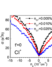
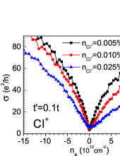
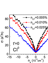
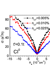
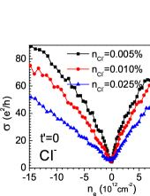
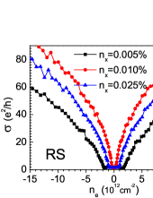
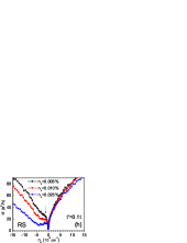
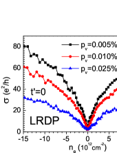
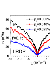
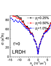
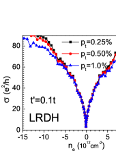
Figure 1: (Color online) The dc conductivity as a function of carrier density $n_{e}$ for disordered graphene. Left panels show the results without the NNN hopping $t^{\prime}$, and right panels with $t^{\prime}=0.1t$. For CI, we use $\kappa=6$ of hexagonal-boron nitride as a typical value of dielectric constant for graphene on a substrate. The use of other $\kappa$ for different substrate such as SiO₂ does not change the results quantitatively. Here $0.01\%$ disorder corresponds to a concentration of $3.82\times 10^{11}cm^{-2}$.

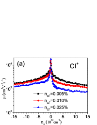
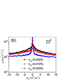
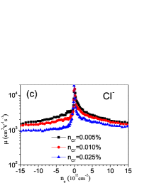
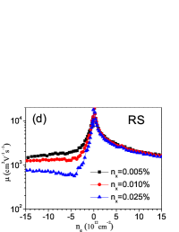
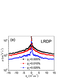
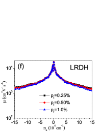
Figure 2: (Color online) The carrier mobility as a function of carrier density $n_{e}$ for disorder graphene with $t^{\prime}$.

The dominant source of disorder which limits the transport and optical properties of graphene is still under debate. Different mechanisms have been proposed and investigated intensively, including charged impurities, random strain fluctuations and resonant scatterers (for reviews see Refs. Peres, 2010; Katsnelson, 2012). Early on, charged impurities (CI) have been recognized as the dominate disorders due to graphene’s unusual linear carrier-density-dependent conductivity. However, this mechanism does not explain the experimental observations that the transport properties of certain samples are not sensitive to the substrate screening Ponomarenko et al. (2009); Couto et al. (2011). On the other hand, strain fluctuations (SF) induced e.g. ripples can be alternative scattering mechanism  Katsnelson and Geim (2008); they can be also responsible for charge inhomogeneities, that is, electron-hole puddles Gibertini et al. (2010, 2012). There is experimental evidence, based on the correlation between the carrier mobility and the width of the resistance peak around charge neutrality, that the long-range disorder potential (LRDP) due to SF could be the dominant source of disorder in high-quality graphene on a substrate Couto et al. (2014). In addition, the SF modulate the electron hopping energies between different atomic sites, inducing the long-range disorder hopping (LRDH), leading to the appearance of the (pseudo) vector potential Katsnelson (2012); Vozmediano et al. (2010). Another common source of disorder are resonant scatterers (RS) such as chemical species like hydrogen or organic groups, which also lead to a sublinear carrier-density-dependent conductivity and a minimum conductivity plateau around the neutrality point Ni et al. (2010); Wehling et al. (2010).

Besides the transport properties, an important part of our knowledge about the electronic properties derives from the optical spectroscopy measurements Peres (2010); Orlita and Potemski (2010). Infrared spectroscopy experiments allow for the control of interband excitations by means of electrical gating Wang et al. (2008); Li et al. (2008). For doped pristine graphene with nonzero chemical potential $\mu_{F}$, the optical conductivity is a step function $\sigma\left(\omega\right)=\sigma_{0}\Theta\left(\omega-2\mu_{F}\right)$ at zero temperature due to Pauli’s exclusion principle. However, there are experimentally observed background contributions to the optical spectroscopy between $0<\omega<2\mu_{F}$ Li et al. (2008); Chen et al. (2011), which are due to the extra intraband excitations introduced by disorder or many-body effects Ando et al. (2002); Grüneis et al. (2003); Peres et al. (2006); Gusynin et al. (2006); Stauber et al. (2007); Gusynin et al. (2007); Stauber et al. (2008a, b); Min and MacDonald (2009); Li et al. (2008); Mak et al. (2008); Yuan et al. (2011). This opens the possibility to identify the source of disorder via the optical measurements.

Previous theoretical investigation of disorders are mainly based on models without considering the next-nearest-neighbor (NNN) hopping $t^{\prime}$. The breakdown of electron-hole symmetry resulting from $t^{\prime}\not=0$ shifts the position of Dirac point from zero to $3t^{\prime}$ Castro Neto et al. (2009); Katsnelson (2012). Recent quantum capacitance measurements indicate that the value of $t^{\prime}$ is about $0.3eV$ Kretinin et al. (2013), consistent with the values obtained from the density functional calculations. It is generally thought that $t^{\prime}$ has relatively weak effects on the physical properties of graphene at low energies Castro Neto et al. (2009); Katsnelson (2012); Stauber et al. (2008a); Kretinin et al. (2013). In the present paper, we study the electronic, transport and optical properties of graphene with different types of disorders including NNN. We show that $t^{\prime}$ has a negligible effect in combination with long-range disorder such as CI, LRDP and LRDH, but changes the physics dramatically when RS are present. Different sources of disorder can be identified via their fingerprints in the common measurable quantities, such as dc conductivity, carrier mobility, optical spectroscopy and Landau level spectrum  etc. We will use these fingerprints to demonstrate the dominant disorder source in several well-known experimental measurements. The paper is organized as follows. In Section II we gives a description of the tight-binding Hamiltonian of single layer graphene including different types of disorders and NNN. In section III and IV, we discuss the effect of different disorders on the transport and optical properties of graphene. Then, we study the Landau level spectrum and quantum capacitance in the presence of perpendicular magnetic field in section V. Finally, a brief discussion and conclusion, including a list of dominant disorder sources in several experiments, is given in section VI.

II Model and Method

We consider disordered graphene described by the tight-binding (TB) Hamiltonian

$$H=-\sum_{i,j}t_{i,j}c_{i}^{\dagger}c_{j}-\sum_{i,j}{t_{i,j}^{\prime}}c_{i}^{\dagger}c_{j}+\sum_{i}v_{i}c_{i}^{\dagger}c_{i},$$ (1)

where the first sum is taken over nearest neighbors and the second one is over next-nearest neighbors.

For CI, we consider randomly distributed point-like charges at the center of a hexagon of the honeycomb lattice ($\mathbf{r}_{k}$)Pereira et al. (2007), which introduce the Coulomb energy $v_{i}=\sum_{k}\mathop{\mathrm{sign}}\left(k\right)e^{2}/\left(\kappa|\mathbf{r}_{i}-\mathbf{r}_{k}|\right)$ at each site $i$, and the screening effect due to the substrate is taken into account by using the dielectric constant $\kappa$ of the substrate. Here, according the values of $\mathrm{sign}\left(k\right)$ we consider three types of CI: (1) CI⁰ for randomly distributed positive or negative potential caused by charges that the whole sample holds the electric neutrality, (2) CI⁺ for only positive potential and (3) CI^- for only negative ones.

For LRDP, the on-site potential $v_{i}$ follows a corrected Gaussian profile which varies smoothly on the scale of lattice constant as $v_{i}=\sum_{k}U_{k}\exp[-\left|\mathbf{r}_{i}-\mathbf{r}_{k}\right|^{2}/(2d^{2})]$Yuan et al. (2011), where $\mathbf{r}_{k}$ is the $k-th$ Gaussian centers which are randomly distributed on the lattice with probability $p_{v}$, $U_{k}$ represents the strength of the local potential and is uniformly random in the range $[-\Delta_{v},\Delta_{v}],$ and $d$ is interpreted as the effective radius. We use $\Delta_{v}=t$ and $d=5a$ to represent the long-range Gaussian potential. Here $a\approx 1.42$Å is the carbon-carbon distance in the single-layer graphene.

The LRDH is introduced in a similar way as LRDP except that the nearest-neighbor hopping parameters are modified according a correlated Gaussian form via $t_{ij}=t+\sum_{k}T_{k}\exp[-\left|\mathbf{r}_{i}+\mathbf{r}_{j}-2\mathbf{r}_{k}\right|^{2}/\left(8d_{t}^{2}\right)],$where $T_{k}$, $d_{t}$ and $p_{t}\$have similar meanings as in LRDP, and we choose $\Delta_{t}=0.25t$ and $d_{t}=5a$Yuan et al. (2011). We want to emphasis that, although the amplitude ($\Delta$) and radius ($d$) of the Gaussian profile in the LRDH and LRDP are free parameters that can be turned in the tight-binding model, the numerical results show little quantitative difference as long as these parameters are of the same order as the chosen values. In general, an increase (decrease) of the amplitude or radius is equivalent to an increase (decrease) of the disorder concentration.

The hydrogen-like RS is described by the Hamiltonian $H_{RS}=V\sum_{i}\left(d_{i}^{\dagger}c_{i}+\mathrm{h.c}\right)$ Robinson et al. (2008); Wehling et al. (2010); Yuan et al. (2010), where $V$ is the hopping between carbon and adatom. We consider the limiting case with $V\rightarrow\infty$, i.e., the electron at the impurity site is completely localized such that the resonant scatterer behaves like vacancy Wehling et al. (2010). In our calculations, we use $t\approx 2.7$ eV and ${t^{\prime}}=t/10$ for the nearest and next-nearest neighbor hopping parameters, respectively. The spin degree of freedom contributes only through a degeneracy factor and, for simplicity, has been omitted in Eq. (1).

The calculations of the electronic and optical properties are performed by the tight-binding propagation method (TBPM) Hams and De Raedt (2000); Yuan et al. (2010); Wehling et al. (2010); Yuan et al. (2012), which is based on the numerical solution of the time-dependent Schrödinger equation and Kubo’s formula. The advantage of this method is that all the calculated quantities are extracted from the real-space wave propagation without any knowledge of the energy eigenstates. Furthermore one can introduce different kinds of (random) disorder by constructing the corresponding TB model for a sample scaling up to micrometers. For more details about the numerical methods we refer to Refs Yuan et al., 2010, 2011. The simulated graphene sample contains up to $8192\times 8192$ atoms subject to periodic boundary conditions.

III TRANSPORT PROPERTIES

We first consider the carrier-density-dependence of the microscopic conductivity $\sigma\left(n_{e}\right)$ for disordered graphene. The microscopic (or semi-classic) conductivity is calculated from the diffusive region of the charge transport, i.e., when the time-dependent diffusion coefficient reaches its the maximum Cresti et al. (2013); Trambly de Laissardière and Mayou (2013, 2014), and it is comparable to the conductivity extracted from the field-effect measurements. In TBPM, the microscopic conductivity at an energy $E$ is calculated by using the Kubo formula Yuan et al. (2010, 2012)

$$\mathbf{\sigma}\left(E\right) = \underset{\tau}{\max}\frac{\rho\left(E\right)}{\Omega}\int_{0}^{\tau}dt~{}\text{Re}\left[e^{-iEt}\left\langle\varphi\right|Je^{i\mathcal{H}t}J\left|E\right\rangle\right],$$

where $\left|\varphi\right\rangle$ is a normalized random state, $\left|E\right\rangle$ is the normalized quasi-eigenstateYuan et al. (2010), $J$ is the current operator, $\Omega$ is the sample area, and $\rho\left(E\right)$ is the density of states (DOS) calculated viaHams and De Raedt (2000); Yuan et al. (2010)

$$\rho\left(E\right)=\frac{1}{2\pi}\int_{-\infty}^{\infty}e^{iEt}\left\langle\varphi|\varphi(t)\right\rangle dt.$$ (3)

The measured field-effect carrier mobility is related to the microscopic conductivity as $\mu\left(E\right)=\sigma\left(E\right)/en_{e}\left(E\right)$, where the carrier density $n_{e}$ is obtained from the integral of DOS via $n_{e}\left(E\right)=\int_{0}^{E}\rho\left(\varepsilon\right)d\varepsilon$.

From the results shown in Fig. 1, we see that (1) including $t^{\prime}$ has negligible effects for CI, LRDP and LRDH, but the results for RS change dramatically. In the presence of RS, there is a strong electron-hole asymmetry in the carrier-density-dependence of dc conductivity. This is due to the fact that the impurity band created by RS is shifted from the Dirac point to the hole sidePereira et al. (2008), introducing strong electron-hole asymmetry at low energies; (2) as a consequence of this shift the conductivity plateau around the neutrality point is also shifted to the hole side, with an impurity-concentration dependent height and width (for very small concentration of RS, there is just as a kink instead of a plateau, see the point indicated by an arrow in Fig. 1(h)) ; These features can be observed in graphene if the concentration of generic RS is increased by exposing the material to atomic hydrogen Ni et al. (2010). (3) $\sigma\left(n_{e}\right)$ exhibits a sublinear dependence for small concentration for all types of disorders, except for the hole side in the presence of RS; (4) For LRDH, $\sigma\left(n_{e}\right)$ is insensitive to the changes of the disorder concentration ($p_{t}$); (5) No matter whether $t^{\prime}$ is nonzero or not, linear-dependent $\sigma\left(n_{e}\right)$ appears only in CI with large concentration of $n_{C}$ Zhu and Lv (2013), indicating that CI is the dominant source of disorder in the experimental samples which show clearly the linear carrier-density-dependent conductivity (such as K151 in Ref. Tan et al. (2007), and Potassium doped samples in Ref. Chen et al. (2008), etc.), agree with the theoretical prediction that $\sigma\left(n_{e}\right)\propto$ $n_{e}$; (6) The electron-hole asymmetry appears also for larger concentration of CI if there is only one types of charge resource (CI⁺ and CI^-). However, this asymmetry is different from the one due to RS in two aspects: first, for CI there is no kink or plateau in the profile; second, the conductivities on both electron and hole sides decrease significantly with larger concentration of CI; (7) Only in the case of CI⁺ the conductivity on the electron side is smaller than on the hole side with the same concentration of carrier density, which is a unique signature of CI⁺. This is in concert with experiment results Tan et al. (2007); Chen et al. (2011).

The field-effect carrier mobility $\mu$ can be calculated from the conductivity and carrier-density through $\mu=\sigma/en_{e}$. In the following we show only the results with non-zero $t^{\prime}$. From the results presented in Fig. 2, we see that (1) the carrier-dependence of mobility $\mu\left(n_{e}\right)$ is very similar for CI⁰ and LRDP; (2) for LRDH, $\mu\left(n_{e}\right)$ is insensitive to the disorder strength; (3) electron-hole asymmetry appears for CI⁺, CI^- and RS, but only in the case of CI⁺ the electron mobility is smaller than the hole for the same concentration of carrier density; (4) for RS, the mobility on the electron side is insensitive to the impurity concentration, and its value can be one order of magnitude larger than the value on the hole side. For example, considering a RS concentration of $n_{x}=0.025\%$, the electron mobility at carrier density $5\times 10^{12}cm^{-2}$ is about $3,000$ ($cm^{2}V^{-1}s^{-1}$) but the hole mobility for the same carrier density is only $\sim 300$. This significant one order difference of the electron and hole mobility is a unique signature of RS; (5) with RS present, on the hole side, the carrier-density-dependent mobility is not monotonic and $\mu\left(n_{e}\right)$ reaches a minimum at the density corresponding to the tail of the conductivity plateau. However with RS present and $t^{\prime}=0$, the drop of mobility at the minimum is one order of magnitude larger than the experimental result.

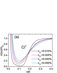
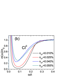
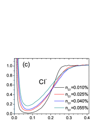
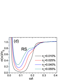
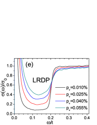
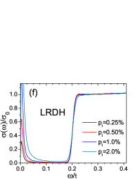
Figure 3: (Color online) The optical conductivity as a function of energy for disordered graphene with $\mu_{F}=0.1t$ and $t^{\prime}=0.1t$. Here $\sigma_{0}=\pi e^{2}/(2h)$ is the universal optical conductivity of graphene. All along the work the temperature of optical calculation is $T=45K$, the same as in the experiment of Ref.Li et al., 2008.

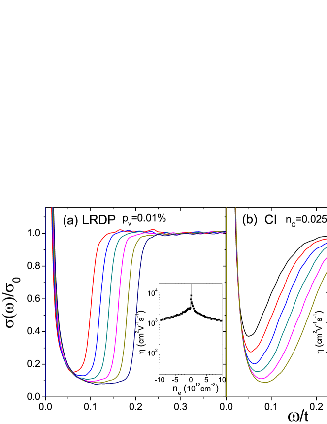
Figure 4: (Color online) The optical conductivity as a function of energy for disordered graphene (a) LRDP, (b) CI, and (c) RS with $t^{\prime}$. The disorder concentrations are determined via the best fit to the experimental results of optical spectroscopy Li et al. (2008); Chen et al. (2011). The chemical potential $\mu_{F}$ changes from $0.05t$ to $0.1t$. The inner panels show the corresponding carrier mobility for the same concentration of disorder. The dashed line in (c) is a guide to eye separating two region in which the spectrum changes differently in the presence of RS.

The minimum conductivity $\sigma_{\min}$ at the Dirac point is of the order of $4e^{2}/h$ for all types of long-range disorders with $t^{\prime}=t/10$. The values of $\sigma_{\min}$ in CI and LRDP do not depend on $t^{\prime}$, but change with the disorder strength such that larger concentration of disorder leads to larger values of $\sigma_{\min}$. This is due to the fact that the increase of potential sources in CI and LRDP will increase the DOS at the $\mu_{F}$, leading to more states which can contribute to the transport. This may also explain the experimental observations in Ref. Tan et al., 2007 and Ref. Geim and Novoselov, 2007 in which the low mobility does not necessary correspond to a smaller value of $\sigma_{\min}$. For LRDH, the value of $\sigma_{\min}$ for $t^{\prime}=0$ is about two time larger than the value for $t^{\prime}=t/10$, but both are insensitive to the disorder strength. For RS and $t^{\prime}=0$, $\sigma_{\min}$ is of the order of $4e^{2}/\pi h$, independent on the impurity concentration $n_{x}$ Cresti et al. (2013); Trambly de Laissardière and Mayou (2013, 2014), but if $t^{\prime}=t/10$, $\sigma_{\min}$ from being of the order of $4e^{2}/h$ at small $n_{x}$ to $4e^{2}/\pi h$ when $n_{x}\geq 0.1\%$, consistent with the numerical results of Ref. Trambly de Laissardière and Mayou, 2014 (data not shown). Thus we conclude that our results indicate that the minimum conductivity $4e^{2}/h$ found in the experiments is dominated by long-range disorder but that the value of $4e^{2}/\pi h$ is due to RS only. It is worth to mention that our consideration does not take into account the effects of weak (anti)localization which can change the behavior of conductance at very large distances Evers and Mirlin (2008), due to energy smearing in our calculations. The latter works as dephasing. At the same time, this dephasing can be physical for real samples.

IV OPTICAL SPECTROSCOPY

The optical conductivity is calculated by using the Kubo formula Ishihara (1971) within TBPMYuan et al. (2010) as (omitting the Drude contribution at $\omega=0$)

$$\sigma\left(\omega\right) = \lim_{\epsilon\rightarrow 0^{+}}\frac{e^{-\beta\omega}-1}{\omega\Omega}\int_{0}^{\infty}e^{-\epsilon t}\sin\omega t$$

$$\times 2~{}\text{Im}\left\langle\varphi|f\left(\mathcal{H}\right)J\left(t\right)\left[1-f\left(\mathcal{H}\right)\right]J|\varphi\right\rangle dt,$$

where $\beta=1/k_{B}T$ is the inverse temperature, $f\left(\mathcal{H}\right)=1/\left[e^{\beta\left(\mathcal{H}-\mu_{F}\right)}+1\right]$ is the Fermi-Dirac distribution operator. Similar as for the transport properties, our numerical calculations show that $t^{\prime}$ has negligible effects on the optical properties of disordered graphene, except if RS are present. In general, disorder introduces new states which could contribute to the extra intraband excitations Ando et al. (2002); Grüneis et al. (2003); Peres et al. (2006); Gusynin et al. (2006); Stauber et al. (2007); Gusynin et al. (2007); Stauber et al. (2008a, b); Min and MacDonald (2009); Li et al. (2008); Mak et al. (2008); Yuan et al. (2011), and therefore enhances the optical conductivity below $2\mu_{F}$, which might explain the observed background contribution in the optical spectrum for $0<\omega<2\mu_{F}$ Li et al. (2008); Chen et al. (2011). This is confirmed by the optical conductivity of disordered graphene calculations shown in Fig. 3. For disordered graphene with CI (including CI⁰, CI⁺ and CI^-) there is a strong enhancement of the optical conductivity below $2\mu_{F}$ and the enhanced spectrum forms a plateau with disorder-dependent minimum conductivity. For LRDP, there is in addition a disorder-dependent plateau in the optical spectrum below $2\mu_{F}$, which is much wider that the one due to CI. For LRDH, the enhancement of the optical conductivity is much smaller than for other types of disorders. For RS and $t^{\prime}=0$, a disorder-dependent peak appears at $\omega\approx\mu_{F}$, which is due to the enhanced excitations of the midgap states at the Dirac point. This peak disappears for $t^{\prime}=t/10$, and instead, a disorder-dependent narrow plateau appears.

In practice, instead of varying the disorder concentration, it is easier to change the chemical potential by applying an electrical potential to a gate. In order to compare to the experimental data of the spectroscopy measurements Li et al. (2008); Chen et al. (2011) quantitatively, we plot in Fig. 4 the best fit of the optical conductivity for different chemical potentials ranging from $0.05t$ to $0.1t$ (since the results of CI⁰, CI⁺ and CI^- are similar, we present here only the case of CI⁰). The disorder concentrations shown in Fig. 4 are determined by matching the minimum value of the optical conductivity plateau to the one observed Li et al. (2008); Chen et al. (2011), yielding $\sigma_{plateau}$ of the order of $0.1\sigma_{0}$ for $\mu_{F}\approx t/10$. The best match of the disorder concentrations from our simulations is $p_{v}=0.01\%$ for LRDP, $n_{C}=0.025\%$ for CI and $n_{x}=0.025\%$ for RS. A direct comparison of the profile of the spectrum between our simulations and the experiments in Ref. Li et al., 2008; Chen et al., 2011 indicates that LRDP fits best to the experiments. In Ref. Li et al., 2008, the carrier mobility measured for the same device is as high as $8,700cm^{2}V^{-1}s^{-1}$ at carrier densities of $2\times 10^{12}cm^{-2}$, and the LRDP also gives the highest mobility that it can reach $\sim 3,000$. For CI, $\mu\sim 1500$, and for RS the mobility is even smaller: for electrons it is $\sim 1,000$ and for holes $\sim 300$. Therefore we conclude that the background contribution of the optical conductivity below $2\mu_{F}$ as observed in Ref. Li et al., 2008 should be due mainly to the presence of LRDP.

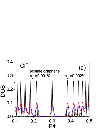
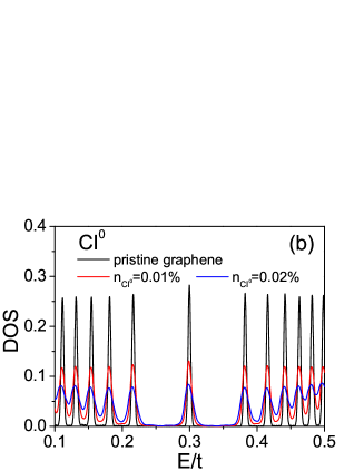
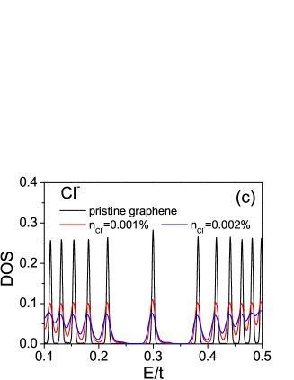
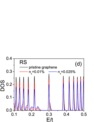
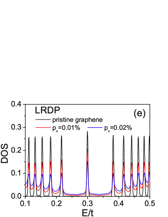
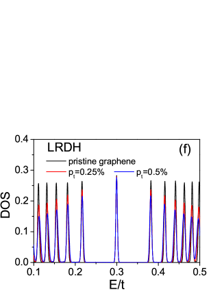
Figure 5: (Color online) Density of states as a function of energy for disordered graphene in the presence of a uniform perpendicular magnetic field ($B=50$T).

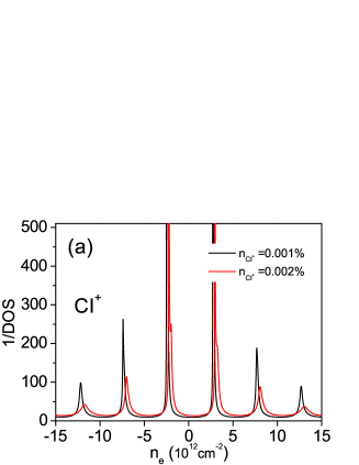
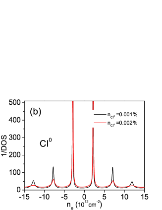
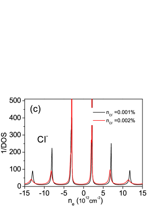
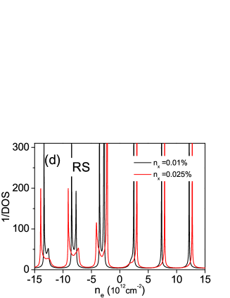
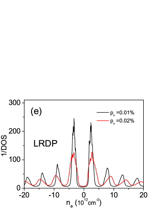
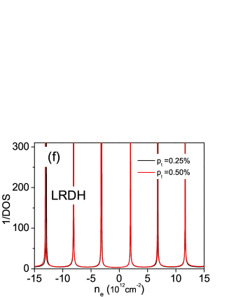
Figure 6: (Color online) The reciprocal of DOS as a function of carry density $n_{e}$ for disordered graphene in the presence of a uniform perpendicular magnetic field ($B=50$T).

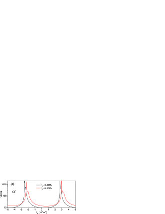
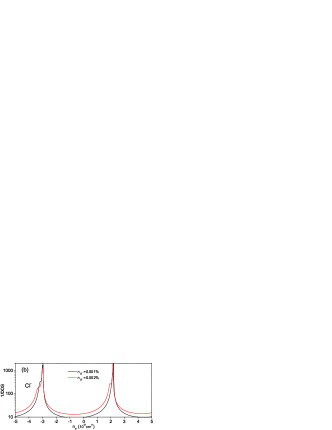
Figure 7: (Color online) The reciprocal of DOS as a function of carry density $n_{e}$ for disordered graphene in the presence of a uniform perpendicular magnetic field ($B=50$T).

V LANDAU LEVEL SPECTRUM

Finally we consider the electronic properties of graphene under a perpendicular magnetic field ($B=50$T). The Landau quantization of the energy levels leads to separated peaks, as shown in Fig. 5. In the presence of disorder, the peak amplitudes of the Landau levels (LL) are reduced and the peaks become broader, except for LRDH in which the influence of disorder is much weaker than for other types of disorders. The peak profiles depend on the different sources of disorder. In general, for long range disorder, the peak is still symmetric along its center, but for RS, the changes are mainly restricted on the side with higher energy. Furthermore, the LL spectrum exhibits electron-hole symmetry for CI⁰ and LRDP, but becomes asymmetric for CI⁺, CI^- and RS. Especially, there are two small peaks around the first Landau level on the hole side shown in Fig. 5(d), which has the same origin as for the zero LL peaks, induced by RS Yuan et al. (2010). The differences that appear in the LL spectrum also appear in quantum capacitance measurement, as the inverse of the latter is proportional to DOS Fang et al. (2007); Xia et al. (2009); Dröscherscher et al. (2010); Wang et al. (2014). Therefore, we also expect a huge effect of RS on the asymmetric quantum Hall conductivity, a topic for future research.

The quantum capacitance $C_{q}$, which is defined as $C_{q}=\rho e^{2}$, can be extracted experimentally from the total capacitance $C$ and the geometry capacitance $C_{g}$ via $1/C_{q}=1/C-1/C_{g}$. In Fig. 6 we show the carrier dependence of $1/\rho$, which is proportional to $1/C_{q}$, for different types of disorders under the same magnetic field ($B=50$T). Due to the presence of disorder, the peak amplitudes decrease significantly except for the LRDH, in which the influence of random hopping is negligible. The change of the spectrum profile for each type of disorder has similar feature deduced from the corresponding DOS. Furthermore, some characters become even more clear in the spectrum of $1/\rho$. For example, the electron-hole asymmetry appeared in the presence of single-type charge impurities (CI⁺ or CI^-) is very special: the slopes of the peaks on the hole and electron sides point to the same direction, depending on the sign of CI (see a zoom of the first two peaks in Fig. 7). This unique feature has also been observed in the experiments.

Ref. disorder Fingerprints [Couto et al., 2014] LRDP Symmetrical $\sigma\left(n_{e}\right)$ in Fig.2 (a), the minimum conductivity plateau in Fig. 2 (b), and the relation of mobility $\mu$ versus $n^{*}$ in Fig. 2 (c). [Ni et al., 2010] RS Asymmetrical $\sigma\left(n_{e}\right)$ of the blue and red curves in Fig. 2 (a). [Li et al., 2008] LRDP A plateau in the doped optical spectroscopy in Fig. 2 (b), together with the corresponding relatively high mobility. [Chen et al., 2011] CI⁺ A narrow plateau in the doped optical spectroscopy, together with a shift of the minimum conductivity to the electron side in Fig. 1. [Tan et al., 2007] CI⁺ The electron mobility is smaller than the hole one in Fig. 2 for samples K130, K145, K151; The minimum conductivity shifts to the electron side in Fig. 3. [Chen et al., 2008] CI^- The hole conductivity is smaller than electron one and the minimum conductivity shifts to the hole side in Fig. 2. [Bolotin et al., 2008] CI⁺ The hole conductivity is larger than electron one in Fig. 1 (the sample before annealing). [Ren et al., 2012] CI A narrow plateau in the doped optical spectroscopy in Fig. 3 (b).

Table 1: List of the dominant disorder source in different experimental samples, identified by using the fingerprints appeared in the transport or optical properties. The figures indicated in the table are these in the corresponding reference.

VI DISCUSSION AND CONCLUSION

We have studied the effects of different types of disorders on the electronic, transport and optical properties of graphene. By comparing the results with and without the NNN hopping, we find that the NNN hopping has negligible effect in combination with long-range disorder such as CI, LRDP and LRDH, but that it changes the physical properties dramatically if RS are present. In the latter case, we find that 1) there is an extra conductivity plateau on the hole side, with a value larger than the minimum conductivity at the neutrality point; 2) the carrier-density-dependent mobility does not always drop with larger carrier density but instead, it reaches a minimum at the edge of the conductivity plateau. 3) a strong electron-hole asymmetry appears in the carrier-density-dependent transport properties and Landau level spectrum; 4) the minimum conductivity at the shifted Dirac point is no longer a constant, but drops to $4e^{2}/\pi h$ when the impurity concentration is larger than $0.05\%$. For long-range disorder, the minimum conductivity for $t^{\prime}=t/10$ is of the order of $4e^{2}/h$ and increases with larger disorder concentration for CI and LRDP, but remains the same for LRDP. The mobility always becomes smaller with larger concentration of disorder, however, the minimum conductivity does not follow the same rule, consistent with the transport measurement Tan et al. (2007); Geim and Novoselov (2007). For doped graphene, the presence of disorder introduces extra excitations below $2\mu_{F}$ but the profiles of the optical spectra are different for different types of disorders.

As an example of using the fingerprints discussed in the main text, we collect the dominant source of disorder in several well-known experiments and list them in Table I. Different types of disorders such as CI (including CI⁰, CI⁺ and CI^-), LRDP and RS have been identified in different experiments, except for the LRDH which has been proved to have negligible influence to the electronic properties. The results obtained in Table I also suggest the dominant source of disorder may vary from sample to sample.

In summary, we suggest that the different but characteristic features that appear in the calculated electronic, transport and optical properties can be used as fingerprints to identify the dominant sources of disorder in graphene.

VII ACKNOWLEDGMENTS

We thank the European Union Seventh Framework Programme under grant agreement n604391 Graphene Flagship. The support by the China Scholarship Council (CSC) and by the Stichting Fundamenteel Onderzoek der Materie (FOM) and the Netherlands National Computing Facilities foundation (NCF) are acknowledged. S.Y. and M.I.K. thank financial support from the European Research Council Advanced Grant program (contract 338957).

References

- Peres (2010) N. M. R. Peres, Rev. Mod. Phys. 82, 2673 (2010).
- Katsnelson (2012) M. I. Katsnelson, Graphene: Carbon in Two Dimensions (Cambridge University Press, 2012).
- Ponomarenko et al. (2009) L. A. Ponomarenko, R. Yang, T. M. Mohiuddin, M. I. Katsnelson, K. S. Novoselov, S. V. Morozov, A. A. Zhukov, F. Schedin, E. W. Hill, and A. K. Geim, Phys. Rev. Lett. 102, 206603 (2009).
- Couto et al. (2011) N. J. G. Couto, B. Sacépé, and A. F. Morpurgo, Phys. Rev. Lett. 107, 225501 (2011).
- Katsnelson and Geim (2008) M. Katsnelson and A. Geim, Phil. Trans. R. Soc. A 366, 195 (2008).
- Gibertini et al. (2010) M. Gibertini, A. Tomadin, M. Polini, A. Fasolino, and M. I. Katsnelson, Phys. Rev. B 81, 125437 (2010).
- Gibertini et al. (2012) M. Gibertini, A. Tomadin, F. Guinea, M. I. Katsnelson, and M. Polini, Phys. Rev. B 85, 201405 (2012).
- Couto et al. (2014) N. J. G. Couto, D. Costanzo, S. Engels, D.-K. Ki, K. Watanabe, T. Taniguchi, C. Stampfer, F. Guinea, and A. F. Morpurgo, Phys. Rev. X 4, 041019 (2014).
- Vozmediano et al. (2010) M. A. H. Vozmediano, M. I. Katsnelson, and F. Guinea, Physics Reports 496, 109 (2010).
- Ni et al. (2010) Z. Ni, L. Ponomarenko, R. Nair, R. Yang, S. Anissimova, I. Grigorieva, F. Schedin, P. Blake, Z. Shen, E. Hill, et al., Nano letters 10, 3868 (2010).
- Wehling et al. (2010) T. O. Wehling, S. Yuan, A. I. Lichtenstein, A. K. Geim, and M. I. Katsnelson, Phys. Rev. Lett. 105, 056802 (2010).
- Orlita and Potemski (2010) M. Orlita and M. Potemski, Semiconductor Science and Technology 25, 063001 (2010).
- Wang et al. (2008) F. Wang, Y. Zhang, C. Tian, C. Girit, A. Zettl, M. Crommie, and Y. R. Shen, Science 320, 206 (2008).
- Li et al. (2008) Z. Li, E. A. Henriksen, Z. Jiang, Z. Hao, M. C. Martin, P. Kim, H. Stormer, and D. N. Basov, Nature Physics 4, 532 (2008).
- Chen et al. (2011) C.-F. Chen, C.-H. Park, B. W. Boudouris, J. Horng, B. Geng, C. Girit, A. Zettl, M. F. Crommie, R. A. Segalman, S. G. Louie, et al., Nature 471, 617 (2011).
- Ando et al. (2002) T. Ando, Y. Zheng, and H. Suzuura, Journal of the Physical Society of Japan 71, 1318 (2002).
- Grüneis et al. (2003) A. Grüneis, R. Saito, G. G. Samsonidze, T. Kimura, M. A. Pimenta, A. Jorio, A. G. S. Filho, G. Dresselhaus, and M. S. Dresselhaus, Phys. Rev. B 67, 165402 (2003).
- Peres et al. (2006) N. M. R. Peres, F. Guinea, and A. H. Castro Neto, Phys. Rev. B 73, 125411 (2006).
- Gusynin et al. (2006) V. P. Gusynin, S. G. Sharapov, and J. P. Carbotte, Phys. Rev. Lett. 96, 256802 (2006).
- Stauber et al. (2007) T. Stauber, N. M. R. Peres, and F. Guinea, Phys. Rev. B 76, 205423 (2007).
- Gusynin et al. (2007) V. P. Gusynin, S. G. Sharapov, and J. P. Carbotte, International Journal of Modern Physics B 21, 4611 (2007).
- Stauber et al. (2008a) T. Stauber, N. M. R. Peres, and A. K. Geim, Phys. Rev. B 78, 085432 (2008a).
- Stauber et al. (2008b) T. Stauber, N. M. R. Peres, and A. H. Castro Neto, Phys. Rev. B 78, 085418 (2008b).
- Min and MacDonald (2009) H. Min and A. H. MacDonald, Phys. Rev. Lett. 103, 067402 (2009).
- Mak et al. (2008) K. F. Mak, M. Y. Sfeir, Y. Wu, C. H. Lui, J. A. Misewich, and T. F. Heinz, Phys. Rev. Lett. 101, 196405 (2008).
- Yuan et al. (2011) S. Yuan, R. Roldán, H. De Raedt, and M. I. Katsnelson, Phys. Rev. B 84, 195418 (2011).
- Castro Neto et al. (2009) A. H. Castro Neto, F. Guinea, N. M. R. Peres, K. S. Novoselov, and A. K. Geim, Rev. Mod. Phys. 81, 109 (2009).
- Kretinin et al. (2013) A. Kretinin, G. L. Yu, R. Jalil, Y. Cao, F. Withers, A. Mishchenko, M. I. Katsnelson, K. S. Novoselov, A. K. Geim, and F. Guinea, Phys. Rev. B 88, 165427 (2013).
- Pereira et al. (2007) V. M. Pereira, J. Nilsson, and A. H. Castro Neto, Phys. Rev. Lett. 99, 166802 (2007).
- Robinson et al. (2008) J. P. Robinson, H. Schomerus, L. Oroszlány, and V. I. Fal’ko, Phys. Rev. Lett. 101, 196803 (2008).
- Yuan et al. (2010) S. Yuan, H. De Raedt, and M. I. Katsnelson, Phys. Rev. B 82, 115448 (2010).
- Hams and De Raedt (2000) A. Hams and H. De Raedt, Phys. Rev. E 62, 4365 (2000).
- Yuan et al. (2012) S. Yuan, T. O. Wehling, A. I. Lichtenstein, and M. I. Katsnelson, Phys. Rev. Lett. 109, 156601 (2012).
- Cresti et al. (2013) A. Cresti, F. Ortmann, T. Louvet, D. Van Tuan, and S. Roche, Phys. Rev. Lett. 110, 196601 (2013).
- Trambly de Laissardière and Mayou (2013) G. Trambly de Laissardière and D. Mayou, Phys. Rev. Lett. 111, 146601 (2013).
- Trambly de Laissardière and Mayou (2014) G. Trambly de Laissardière and D. Mayou, Advances in Natural Sciences: Nanoscience and Nanotechnology 5, 015007 (2014).
- Pereira et al. (2008) V. M. Pereira, J. M. B. Lopes dos Santos, and A. H. Castro Neto, Phys. Rev. B 77, 115109 (2008).
- Zhu and Lv (2013) W. Zhu and B. Lv, Physics Letters A 377, 1649 (2013).
- Tan et al. (2007) Y.-W. Tan, Y. Zhang, K. Bolotin, Y. Zhao, S. Adam, E. H. Hwang, S. Das Sarma, H. L. Stormer, and P. Kim, Phys. Rev. Lett. 99, 246803 (2007).
- Chen et al. (2008) J.-H. Chen, C. Jang, S. Adam, M. Fuhrer, E. Williams, and M. Ishigami, Nature Physics 4, 377 (2008).
- Geim and Novoselov (2007) A. K. Geim and K. S. Novoselov, Nature materials 6, 183 (2007).
- Evers and Mirlin (2008) F. Evers and A. D. Mirlin, Rev. Mod. Phys. 80, 1355 (2008).
- Ishihara (1971) A. Ishihara, Statistical Physics (Academic Press, New York, 1971).
- Fang et al. (2007) T. Fang, A. Konar, H. Xing, and D. Jena, Applied Physics Letters 91, 092109 (2007).
- Xia et al. (2009) J. Xia, F. Chen, J. Li, and N. Tao, Nature Nanotech. 4, 505 (2009).
- Dröscherscher et al. (2010) S. Dröscherscher, P. Roulleau, F. Molitor, P. Studerus, C. Stampfer, K. Ensslin, and T. Ihn, Appl. Phys. Lett 96, 152104 (2010).
- Wang et al. (2014) L. Wang, X. Chen, W. Zhu, Y. Wang, C. Zhu, Z. Wu, Y. Han, M. Zhang, W. Li, Y. He, et al., Phys. Rev. B 89, 075410 (2014).
- Bolotin et al. (2008) K. I. Bolotin, K. J. Sikes, J. Hone, H. L. Stormer, and P. Kim, Phys. Rev. Lett. 101, 096802 (2008).
- Ren et al. (2012) L. Ren, Q. Zhang, J. Yao, Z. Sun, R. Kaneko, Z. Yan, S. Nanot, Z. Jin, I. Kawayama, M. Tonouchi, et al., Nano letters 12, 3711 (2012).