Solar wind turbulence from MHD to sub-ion scales: high-resolution hybrid simulations

Abstract

We present results from a high-resolution and large-scale hybrid (fluid electrons and particle-in-cell protons) two-dimensional numerical simulation of decaying turbulence. Two distinct spectral regions (separated by a smooth break at proton scales) develop with clear power-law scaling, each one occupying about a decade in wave numbers. The simulation results exhibit simultaneously several properties of the observed solar wind fluctuations: spectral indices of the magnetic, kinetic, and residual energy spectra in the magneto-hydrodynamic (MHD) inertial range along with a flattening of the electric field spectrum, an increase in magnetic compressibility, and a strong coupling of the cascade with the density and the parallel component of the magnetic fluctuations at sub-proton scales. Our findings support the interpretation that in the solar wind large-scale MHD fluctuations naturally evolve beyond proton scales into a turbulent regime that is governed by the generalized Ohm’s law.

1. Introduction

In-situ measurements of the solar wind plasma and electromagnetic field show spectra with a power-law scaling spanning several decades in frequency, $f$ (e.g. Alexandrova et al., 2009; Sahraoui et al., 2010; Roberts, 2010). Power-laws support an interpretation in term of turbulent fluctuations, although the rich variety of spectral features is not easily explained in the framework of known turbulent theories and phenomenologies.

For frequencies in the so-called magneto-hydrodynamic (MHD) range, $10^{-4}~{}\mathrm{Hz}\lesssim f\lesssim 10^{-2}~{}\mathrm{Hz}$ at $1~{}\mathrm{AU}$, the magnetic field spectrum and the kinetic field spectrum have a different scaling, the former being proportional to $f^{-5/3}$ while the latter to $f^{-3/2}$ (Podesta et al., 2007; Salem et al., 2009; Wicks et al., 2011; Tessein et al., 2009). While a magnetic excess is generally found in solar wind turbulence, only recently the spectrum of residual energy (the difference between magnetic and kinetic energy) was shown to have a power-law scaling with a spectral index $-2$ (Chen et al., 2013a). Such finding confirms early predictions on the residual energy spectrum (Grappin et al., 1983) and numerical results of incompressible MHD simulations (Muller & Grappin, 2005). Note that the three spectral indices ($-3/2,~{}-5/3,~{}-2$) for the kinetic, magnetic, and residual energy spectrum are not reproduced simultaneously in any direct numerical simulation (DNS) (e.g. Muller & Grappin, 2005; Chen et al., 2011b) unless a particular driving is applied to large scales (Boldyrev et al., 2011). Finally, in the MHD range, magnetic and velocity fluctuations are dominated by the transverse components with respect to the ambient magnetic field ${\boldsymbol{B}}_{0}$ (e.g. Smith et al., 2006; Wicks et al., 2011).

Moving to higher frequencies, $f\gtrsim 10^{-2}~{}\mathrm{Hz}$, there is growing evidence that kinetic effects become important and change the nature of the self-similar spectra of fluctuations observed for $f\gtrsim 1~{}\mathrm{Hz}$. A spectral break appears in magnetic and velocity spectra at proton scales, separating the MHD inertial range cascade from a second power-law interval at kinetic scales. The physical scale associated with this spectral break has not been identified yet (e.g. Bourouaine et al., 2012; Bruno & Trenchi, 2014; Chen et al., 2014). The spectral index of magnetic fluctuations after the break varies between $(-4,-2)$ (Leamon et al., 1998; Smith et al., 2006), although it tends to cluster around a slope of $-2.8$ for higher frequencies (Alexandrova et al., 2012). The change in the turbulence regimes also shows up in the density spectrum (Chen et al., 2013b), which steepens and couples to the parallel component of magnetic field. The latter becomes as energetic as the two perpendicular components, resulting in an increase of the so-called magnetic compressibility (Alexandrova et al., 2008; Salem et al., 2012; Kiyani et al., 2013). Finally, measurements at 1 AU show that the spectrum of electric field flattens at about $1~{}\mathrm{Hz}$ (Bale et al., 2005; Kellogg et al., 2006), although the noise level hinders the determination of a precise spectral scaling.

The measure of structure functions of third order at MHD scales (Sorriso-Valvo et al., 2007; MacBride et al., 2008) and of high-order at MHD (Salem et al., 2009) and at sub-proton scales (Kiyani et al., 2013) provided additional evidences that fluctuations are turbulent all the way down to electron scales in the solar wind. While DNS are able to reproduce some aspects of either the MHD range (e.g. Maron & Goldreich, 2001; Mason et al., 2008; Beresnyak & Lazarian, 2009; Grappin & Muller, 2010; Lee et al., 2010; Chen et al., 2011b; Boldyrev et al., 2011; Dong et al., 2014) or the sub-proton range (e.g. Matthaeus et al., 2008; Howes et al., 2011; Markovskii & Vasquez, 2011; Camporeale & Burgess, 2011; Boldyrev et al., 2013; Gary et al., 2012; Wan et al., 2012; Servidio et al., 2012; Meyrand & Galtier, 2013; Passot et al., 2014), to our knowledge a clear indication that a turbulent regime establishes in the whole spectrum spanning the two ranges has never been reported so far.

In this work we present results from a high-resolution hybrid (fluid electrons, particle-in-cell protons) two-dimensional (2D) DNS of turbulence and provide the first direct numerical evidence of the simultaneous occurrence of several features observed in the solar wind spectra. These include i) the different scaling of magnetic and kinetic fluctuations in the MHD range, ii) a magnetic spectrum with a clear double power-law scaling separated by a break, iii) an increase in magnetic compressibility at small scales, iv) a strong coupling between density and magnetic fluctuations at small scales. The electric field spectrum is also consistent with observations, showing a change in the spectral properties at sub-proton scales. Our results indicate that the switch in the spectral slopes observed in the solar wind results from the natural continuation of a large-scale MHD turbulent cascade through proton and down to electron scales, where the different field couplings are governed by the non-ideal terms of the Ohm’s law.

2. Numerical setup

The kinetic model uses the hybrid approximation: electrons are considered as a massless, charge neutralizing, isothermal fluid; ions are described by a particle-in-cell model (see Matthews 1994 for detailed model equations). The characteristic spatial and temporal units used in the model are the proton inertial length $d_{p}=v_{A}/\Omega_{p}$, $v_{A}$ being the Alfvén speed, and the inverse proton gyrofrequency $1/\Omega_{p}$, respectively. We use a spatial resolution $\Delta x=\Delta y=0.125\,d_{p}$, and there are $8000$ particles-per-cell (ppc) representing protons. The resistive coefficient is set to the value $\eta=5~{}10^{-4}~{}4\pi v_{A}c^{-1}\Omega_{p}^{-1}$ to prevent the accumulation of magnetic energy at the smallest scales. Fields and moments are defined on a 2D $x$–$y$ grid with dimensions $2048^{2}$ with periodic boundary conditions. Protons are advanced with a time step $\Delta t=0.025\,\Omega_{p}^{-1}$, while the magnetic field $\boldsymbol{B}$ is advanced with a smaller time step $\Delta t_{B}=\Delta t/10$. The number density $n$ is assumed to be equal for protons and electrons, $n_{p}=n_{e}=n$, and both protons and electrons are isotropic, with $\beta_{p}=\beta_{e}=0.5$ where $\beta_{p,e}=8\pi nK_{B}T_{p,e}/B^{2}_{0}$ are the proton (electron) betas (here $K_{B}$ is the Boltzmann’s constant, $B_{0}$ the ambient magnetic field, and $T_{p,e}$ are the proton and electron temperatures).

We impose an initial ambient magnetic field ${\boldsymbol{B}}_{0}=B_{0}\hat{{\boldsymbol{z}}}$, perpendicular to the simulation plane. We add an initial spectrum of linearly polarized magnetic and bulk velocity fluctuations ${\boldsymbol{u}}$, with only in-plane components. Fourier modes of equal amplitude and random phases are excited in the range $-0.2<k_{x,y}<0.2$, assuring energy equipartition and vanishing correlation between kinetic and magnetic fluctuations. Initial velocity fluctuations have vanishing divergence and density fluctuations are also vanishing (in the limit of numerical noise). Quantities are defined as parallel ($\|$) and perpendicular ($\perp$) with respect to ${\boldsymbol{B}}_{0}$. We define the omnidirectional spectra,

$$E_{\Psi}(k_{\bot})\equiv\delta\Psi^{2}(k_{\bot})/k_{\bot}=\sum_{|{\boldsymbol{k_{\bot}}}|=k_{\bot}}\hat{\Psi}^{2}_{2D}({\boldsymbol{k}}_{\bot}),$$ (1)

where $\hat{\Psi}$ are the Fourier coefficients of a given quantity $\Psi$ (we use ${\boldsymbol{E}}$ and ${\boldsymbol{J}}$ to indicate electric field and current density respectively) and $\delta\Psi(k_{\bot})$ is the amplitude of the fluctuation $\Psi$ at the scale $k_{\bot}$. We also define the root mean square value (rms) as

$$\Psi^{rms}=\sqrt{\langle\Psi^{2}\rangle-\langle\Psi\rangle^{2}}.$$ (2)

where $\langle...\rangle$ stands for a real-space average over the whole simulation domain. With these definitions, the initial conditions have $E_{u}\sim E_{B}\propto k_{\bot}$ with $B^{rms}/B_{0}\sim 0.24$ allowing for a fast turbulent dynamics sustained for about $300~{}\Omega_{p}^{-1}$ (the nominal nonlinear time at the beginning of the simulation is approximately $20~{}\Omega_{p}^{-1}$, but it increases at later time).

3. Results

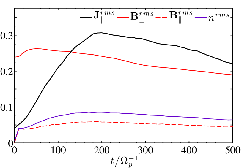
Figure 1.— Root-mean-square parallel current density (black line), perpendicular and parallel magnetic fluctuations (red-solid line and red-dashed lines respectively), and density fluctuations (purple line) as a function of time (normalized to the inverse of the proton gyrofrequency $\Omega_{p}$). As a reference, the nonlinear time at the initial time is about $20~{}\Omega_{p}^{-1}$.

In Figure 1 we plot the rms of the parallel current density, of the parallel and perpendicular magnetic field, and of the density fluctuations. The current density increases until $t=200~{}\Omega_{p}^{-1}$, reflecting the formation of small scales due to the development of a turbulent cascade, and then declines smoothly. The decay is slow, since larger and larger scales continue to feed the cascade at later times. Accordingly the perpendicular magnetic field declines steadily after a transient increase. Shortly after the beginning, fluctuations in the parallel component of magnetic field and in the density appear, slowly increase, reaching a shallow maximum at the same time of the current density, and then decline slowly. The initial growth is due to the generation of a low level of compressive fluctuations. Velocity fluctuations (not shown) behave similarly to magnetic fluctuations, with the perpendicular component declining monotonically (there is no initial growth) and the parallel component originating from compressive effects. In the following we will show spectra at the time of the peak of the current density $t=200~{}\Omega_{p}^{-1}$, but all the turbulent properties are stable and remain valid until the end of the simulation ($t=500~{}\Omega_{p}^{-1}$).

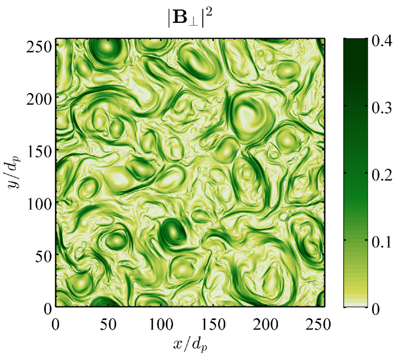
Figure 2.— Contour plot of the perpendicular magnetic energy at $t=200~{}\Omega_{p}^{-1}$.

In Figure 2 we show isocontours of the perpendicular magnetic field energy. This snapshot highlights the formation of intense vortex-like and filamentary structures. The latter reflect the local anisotropy of small scales fluctuations, while their random orientation assures the statistical isotropy of the two-dimensional spectrum: we thus consider in the following only omnidirectional spectra.

In Figure 3 (top panel), we show the spectra of the total velocity, magnetic, and electric field. The magnetic spectrum (red line) has a double power-law scaling, each power-law range occupying about one decade, with a break at $k_{\bot}d_{p}\sim 2$ that separates the MHD from the sub-proton range. The bulk velocity spectrum (blue line) also has a power-law scaling in the MHD range but it falls off abruptly at $k_{\bot}d_{p}\sim 1$, not showing any clear power-law at higher wavenumbers. At smaller scales it reaches the ppc noise level, estimated as the level of velocity fluctuations at $t=0$ (light blue dashed line). Finally the electric field spectrum (green line) follows the velocity in the MHD range ($k_{\bot}d_{p}\lesssim 0.4$) and tends to flatten as it enters the sub-proton range ($k_{\bot}d_{p}\gtrsim 2$).

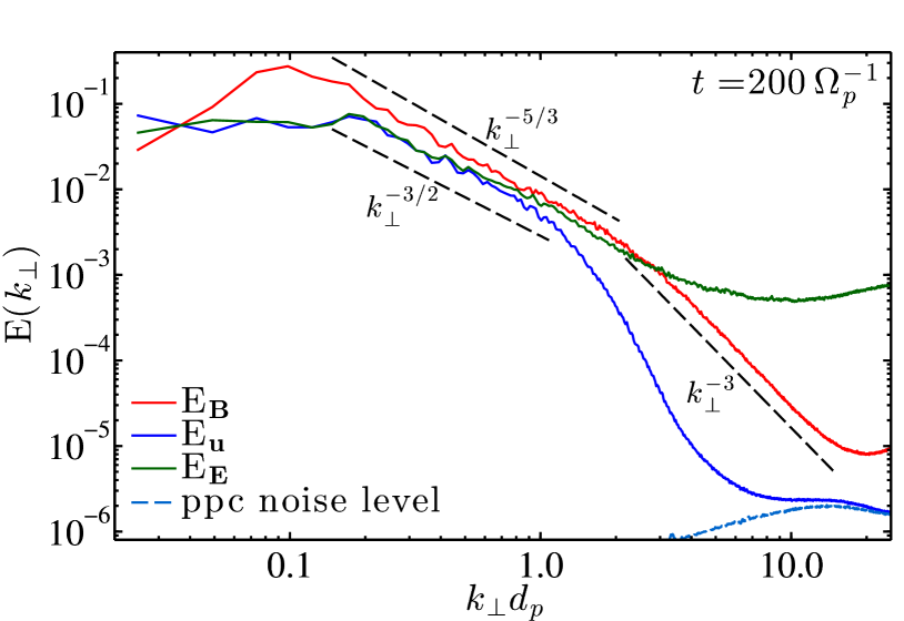
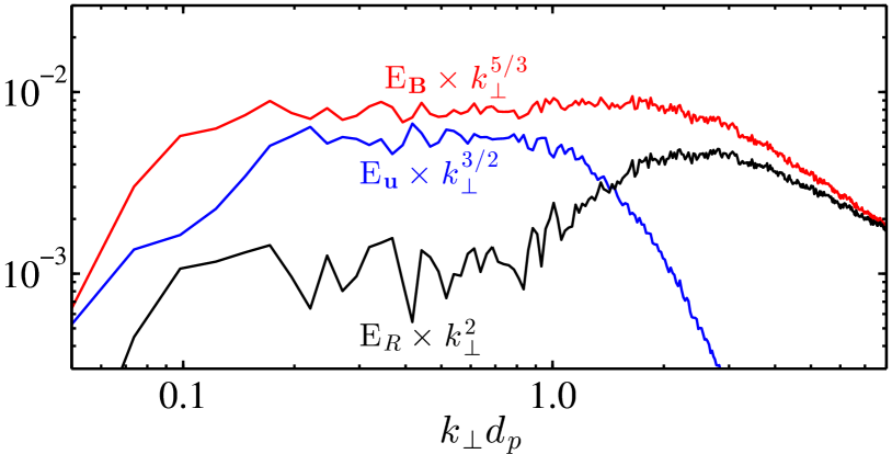
Figure 3.— Top panel. Omnidirectional spectra of total magnetic (red), total kinetic (blue), and total electric field (green) fluctuations versus perpendicular wavenumber $k_{\bot}$ at $t=200~{}\Omega_{p}^{-1}$. The spectrum of kinetic energy at $t=0$ is plotted with a dashed light-blue line as an indicator of ppc noise level.Dashed black lines are references for the corresponding spectral indices. Bottom panel. Magnetic (red), kinetic (blue) and residual energy (black) spectra compensated by $k_{\bot}^{5/3}$, $k_{\bot}^{3/2}$ and $k_{\bot}^{2}$, respectively.

These spectral properties are qualitatively and quantitatively in agreement with observed solar wind spectra. In the MHD range the magnetic and kinetic spectra are power-laws with scaling consistent with $E_{B}\propto k_{\bot}^{-5/3}$ and $E_{u}\propto k_{\bot}^{-3/2}$, respectively, as can be seen in the bottom panel of Figure 3 where the spectra are compensated by $k^{5/3}$ and $k^{3/2}$ respectively. In the same panel we also plot the residual energy spectrum, $E_{R}=E_{B}-E_{u}$, which has a power-law scaling over about one decade in the MHD range with a spectral index $\approx-2$ as in observations (Chen et al., 2013a). In addition, in the sub-proton range the magnetic spectrum scales as $E_{B}\propto k_{\bot}^{-3}$, a spectral index which is very close to the value $-2.8$ reported in observations (Alexandrova et al., 2009). Note that the electric field spectrum is strongly coupled to the bulk velocity spectrum at MHD scales (they are basically indistinguishable for $k_{\bot}d_{p}\lesssim 0.4$), reflecting the dominance of the ideal MHD term ($|{\boldsymbol{u}}\times{\boldsymbol{B}}|\sim B_{0}\,u_{\perp}$) in the generalized Ohm’s law, and consistent with solar wind observations (Chen et al., 2011a). At smaller scales, it decouples from the velocity spectrum since the Hall term (${\boldsymbol{J}}\times{\boldsymbol{B}}/n$) and the electron pressure gradient term ($\boldsymbol{\nabla}P_{e}/n$) start to dominate.

Since both other fields and derivatives enter in its computation, ${\boldsymbol{E}}$ is the field that is mostly affected by numerical effects and it’s not straightforward to give a simple estimate of its noise level, as done for the velocity field. Ultimately, we can reasonably claim that the shallower slope of its spectrum for $2\lesssim k_{\bot}d_{p}\lesssim 7$ is of physical nature, while its behavior at smaller scales is most likely not. On the contrary, quantitative results for the spectra of magnetic and density fluctuations are more robust even at larger wave numbers. A detailed description and discussion about different sources of numerical noise, e.g. the finite number of ppc, will be given in a companion paper (Franci et al., 2015). For the purpose of this Letter, what matters is that such numerical noise does not affect either the qualitative scaling of the electric field spectrum for $k_{\bot}d_{p}\lesssim 7$ or the estimate of the spectral indices of other fields up to $k_{\bot}d_{p}\sim 10$ (except the velocity field which is presumably affected by the noise level at $k_{\bot}d_{p}\gtrsim 4$).

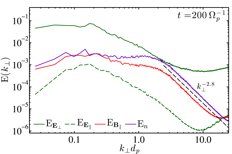
Figure 4.— Omnidirectional spectra of density (purple line), parallel magnetic field (red line), parallel and perpendicular electric field (green dashed and solid line, respectively) versus perpendicular wavenumber $k_{\bot}$ at $t=200~{}\Omega_{p}^{-1}$.

The transition from the MHD regime to the sub-proton regime is not only characterized by a change in the spectral indices, but also by an increase of energy of the parallel magnetic field and the density fluctuations relative to other fields. These are shown in Figure 4, along with the parallel and the perpendicular electric field spectrum. The density and parallel magnetic fluctuations are coupled in the whole range of scales. In the MHD range, they have a flat spectrum that is an order of magnitude smaller than the perpendicular electric field. This also results in a small power in the spectrum of the total magnetic field intensity $E_{|B|}<E_{B}$ (not shown), consistently with solar wind observations (Horbury & Balogh, 2001). In the sub-proton range, $E_{B\|}$ and $E_{n}$ steepen, both having a clear power-law scaling with index $-2.8$. By comparing Figures 3-4 one can see that the parallel and perpendicular components of magnetic fluctuations become comparable at the sub-proton scales, leading also to $E_{|B|}\sim E_{B}$. Concerning the electric field spectrum, at all scales the perpendicular component $E_{E\bot}$ dominates by a factor $\sim 100$ the parallel component $E_{E\|}$, reflecting the fact that in our configuration the leading terms of the generalized Ohm’s law are linear and quadratic in the fluctuations’ amplitude for $E_{E\bot}$ and $E_{E\|}$ respectively. Note that $E_{E\bot}$ flattens at the sub-proton scales and $E_{E\|}$ steepens in qualitative agreement with observations (Mozer & Chen, 2013). It is hard to determine the spectral index of $E_{E\bot}$ at sub-proton scales; a rough estimate gives $\propto k_{\bot}^{-0.8}$, consistent with ${\boldsymbol{E}}$ being determined by the Hall and pressure terms. In fact, retaining only the leading order in the expression of ${\boldsymbol{E}}$ one gets $E_{E}\sim E_{E\bot}\propto k_{\bot}^{2}E_{B_{\|},n}\sim k_{\bot}^{-0.8}$.

We can further compare our results with observations considering three non-dimensional ratios involving density, magnetic and electric field fluctuations shown in Figure 5. Consider first the magnetic compressibility, the ratio of parallel to total magnetic fluctuations (red line). It is negligible in the MHD range, increases while approaching the sub-proton scales, and finally saturates to a level $\delta B_{||}/\delta B\sim 0.5$. Thus, magnetic fluctuations have mainly perpendicular components in the MHD range but tend to become isotropic at small scales, approaching a value $\delta B_{||}^{2}\sim\delta B_{\bot}^{2}/3$, which is within the range ($\sim 0.2\div 0.5$) measured in the solar wind at spacecraft frequencies larger then $1~{}\mathrm{Hz}$ (Kiyani et al., 2013). This is also in very good agreement with the level of magnetic compressibility expected for kinetic Alfvén wave turbulence for the parameters adopted in our simulation (e.g. Boldyrev et al., 2013).

The purple line in Figure 5 shows the ratio of normalized density fluctuations over normalized perpendicular magnetic fluctuations, $\delta\tilde{n}/\delta\tilde{B_{\bot}}$, where $\delta\tilde{B}_{\bot}=\delta B_{\bot}/B_{0}$ and $\delta\tilde{n}=\Gamma\delta n/n_{o}$ respectively, and $\Gamma$ ($3/4$ in our simulation) is a non-dimensional kinetic normalization that depends on $T_{p},T_{e},\beta_{p},v_{A}$ (Schekochihin et al., 2009; Boldyrev et al., 2013). With this normalization $\delta B_{\perp}$ and $\delta n$ are expected to have the same amplitude for kinetic Alfvénic fluctuations. Indeed $\delta\tilde{n}/\delta\tilde{B_{\bot}}$ increases and then saturates at a value $\sim 1$ at sub-proton scales. Note that the plateau and its value $\sim 1$ are consistent with observations (on average $\delta\tilde{n}/\delta\tilde{B}_{\bot}=0.75$, cf. Chen et al. 2013b).

Finally, we plot the ratio between the perpendicular electric fluctuations (normalized by the Alfvén speed) and the perpendicular magnetic fluctuations (green line). Similarly to the observed frequency spectra in the solar wind frame (Bale et al., 2005), this ratio is about $1$ in the MHD range, where the MHD term (${\boldsymbol{u}}\times{\boldsymbol{B}}$) dominate. At $k_{\bot}d_{p}\sim 1$ the ratio increases reflecting the role of the Hall term (${\boldsymbol{J}}\times{\boldsymbol{B}}/n$) and the pressure gradient term ($\boldsymbol{\nabla}P_{e}/n$) in the generalized Ohm’s law.

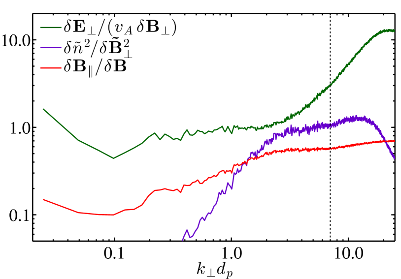
Figure 5.— Ratio of perpendicular electric field to perpendicular magnetic field (green), ratio between normalized density and perpendicular magnetic fluctuations (purple, see text for the normalizations), and ratio of parallel to total magnetic field fluctuations (magnetic compressibility, red). The numerical noise affects the ratios for $k_{\bot}d_{p}\gtrsim 7$ (vertical dotted line).

4. Conclusion

In this Letter we show that hybrid 2D large-scale, high-resolution simulations of turbulence are able to reproduce simultaneously several aspects of the MHD range and of the sub-proton range of solar wind spectra.

Two noticeable examples are given by the spectra of the magnetic field and of the electric field. The former displays a clear double power-law scaling, with spectral indices $-5/3$ and $-3$ in the MHD and sub-proton range respectively, separated by a smooth break at $k_{\bot}d_{p}\sim 2$. The electric field spectrum also shows a change in the spectral properties at about the same scales, being coupled to velocity fluctuations in the MHD range, and becomes shallower at sub-proton scale. It is also worth noting that in the MHD range we found the scaling observed in the solar wind for the magnetic, kinetic, and residual energy spectra (respectively $-5/3,~{}-3/2$, and $-2$). To our knowledge this is the first time that these spectral indices are obtained for turbulence with vanishing correlation between magnetic and velocity fields. DNS of incompressible MHD usually capture only the scaling of the residual energy and the total energy (Muller & Grappin, 2005) while Reduced MHD fails in reproducing velocity and kinetic spectral indices (Chen et al., 2011b) or requires special driving (Boldyrev et al., 2011). This may indicate that it is necessary to go beyond the incompressible MHD approximation even in the inertial range. Further work is needed to test this possibility, extending the analysis to a full 3D simulation.

In the sub-proton scales we found an increase in magnetic compressibility and a strong coupling between density and the parallel component of magnetic fluctuations - both having the same spectral index of $-2.8$ - with the main cascade of $E_{B_{\perp}}$ driven from the MHD scales. All these spectral indices match or are consistent with observations. The only relevant discrepancies are the flat spectra (slope $\sim 0$) of parallel magnetic fluctuations and density fluctuations in the MHD range. In the solar wind they have a spectral index $-5/3$ (e.g. Chen et al., 2012). This aspect is not fully captured by our simulations probably because of the limited compressibility imposed by the 2D dynamics and/or by the value of the proton $\beta$. Note however that this does not prevent the full development of a compressible cascade at kinetic scales, in good agreement with observations.

Properties shown in Figure 5 are consistent with the turbulence at sub-proton scales being ruled by fluctuations with properties of kinetic Alfvén waves. However, note that the level of magnetic and gas compressibility expected for this regime follows from more general properties of the thermodynamical state assumed for the plasma ($\beta_{e}$, $\beta_{p}$ and ion-electron temperature ratio), which govern the couplings between the different fields $B$, $E$ and $n$ via the generalized Ohm’s law. In the low-frequency regime (i.e. below the whistler range), the ratios $\delta\tilde{n}^{2}/\delta{\boldsymbol{B}}_{\bot}^{2}$, $\delta{\boldsymbol{B}}_{\|}/\delta{\boldsymbol{B}}$ are not expected to depend on $k$ (Boldyrev et al., 2013) since they do not rely on the specific dispersion relation of the fluctuations. In this sense, the plateaus at $2\lesssim k_{\bot}\lesssim 7$ in Figure 5 represent a more general and likely universal manifestation of low-frequency turbulence at kinetic scale, and this is how we intend to present them here.

As a concluding remark, we stress that our simulation implements a finite resistivity to assure a source of damping at small scales for the magnetic fluctuations, and thus to prevent energy accumulation and the consequent artificial flattening of the spectrum. Although a more detailed and quantitative analysis of the related effects will be given in a forthcoming paper (Franci et al., 2015), we anticipate that the values of resistivity and the number of ppc affect the ion heating properties.

Acknowledgments This project has received funding from the European Union’s Seventh Framework Programme for research, technological development and demonstration under grant agreement No. 284515 (SHOCK). Website: project-shock.eu/home/. AV acknowledges the Interuniversity Attraction Poles Programme initiated by the Belgian Science Policy Office (IAP P7/08 CHARM). LM was funded by STFC grant ST/K001051/1. PH acknowledges GACR grant 15-10057S. HPC resources were provided by CINECA (grant 2014 HP10CLF0ZB and HP10CNMQX2M). We warmly thank Frank Löffler for providing HPC resources through the Louisiana State University (allocation hpc$\_$hyrel14).

References

- Alexandrova et al. (2008) Alexandrova, O., Carbone, V., Veltri, P., & Sorriso-Valvo, L. 2008, ApJ, 674, 1153
- Alexandrova et al. (2012) Alexandrova, O., Lacombe, C., Mangeney, A., Grappin, R., & Maksimovic, M. 2012, ApJ, 760, 121
- Alexandrova et al. (2009) Alexandrova, O., Saur, J., Lacombe, C., Mangeney, A., Mitchell, J., Schwartz, S. J., & Robert, P. 2009, PhRvL, 103, 165003
- Bale et al. (2005) Bale, S. D., Kellogg, P. J., Mozer, F. S., Horbury, T. S., & Reme, H. 2005, PhRvL, 94, 215002
- Beresnyak & Lazarian (2009) Beresnyak, A., & Lazarian, A. 2009, ApJ, 702, 1190
- Boldyrev et al. (2013) Boldyrev, S., Horaites, K., Xia, Q., & Perez, J. C. 2013, ApJ, 777, 41
- Boldyrev et al. (2011) Boldyrev, S., Perez, J. C., Borovsky, J. E., & Podesta, J. J. 2011, ApJL, 741, L19
- Bourouaine et al. (2012) Bourouaine, S., Alexandrova, O., Marsch, E., & Maksimovic, M. 2012, ApJ, 749, 102
- Bruno & Trenchi (2014) Bruno, R., & Trenchi, L. 2014, ApJL, 787, L24
- Camporeale & Burgess (2011) Camporeale, E., & Burgess, D. 2011, ApJ, 730, 114
- Chen et al. (2011a) Chen, C. H. K., Bale, S. D., Salem, C., & Mozer, F. S. 2011a, ApJL, 737, L41
- Chen et al. (2013a) Chen, C. H. K., Bale, S. D., Salem, C. S., & Maruca, B. A. 2013a, ApJ, 770, 125
- Chen et al. (2013b) Chen, C. H. K., Boldyrev, S., Xia, Q., & Perez, J. C. 2013b, PhRvL, 110, 225002
- Chen et al. (2014) Chen, C. H. K., Leung, L., Boldyrev, S., Maruca, B. A., & Bale, S. D. 2014, GeoRL, 41, 8081
- Chen et al. (2011b) Chen, C. H. K., Mallet, A., Yousef, T. A., Schekochihin, A. A., & Horbury, T. S. 2011b, MNRAS, 415, 3219
- Chen et al. (2012) Chen, C. H. K., Salem, C. S., Bonnell, J. W., Mozer, F. S., & Bale, S. D. 2012, PhRvL, 109, 035001
- Dong et al. (2014) Dong, Y., Verdini, A., & Grappin, R. 2014, ApJ, 793, 118
- Franci et al. (2015) Franci, L., Landi, S., Matteini, L., Hellinger, P., & Verdini, A. 2015, ApJ, to be submitted
- Gary et al. (2012) Gary, S. P., Chang, O., & Wang, J. 2012, ApJ, 755, 142, 142
- Grappin et al. (1983) Grappin, R., Leorat, J., & Pouquet, A. 1983, A&A, 126, 51
- Grappin & Muller (2010) Grappin, R., & Muller, W.-C. 2010, PhRvE, 82, 26406
- Horbury & Balogh (2001) Horbury, T. S., & Balogh, A. 2001, JGR, 106, 15929
- Howes et al. (2011) Howes, G. G., Tenbarge, J. M., Dorland, W., Quataert, E., Schekochihin, A. A., Numata, R., & Tatsuno, T. 2011, PhRvL, 107, 035004
- Kellogg et al. (2006) Kellogg, P. J., Bale, S. D., Mozer, F. S., Horbury, T. S., & Reme, H. 2006, ApJ, 645, 704
- Kiyani et al. (2013) Kiyani, K. H., Chapman, S. C., Sahraoui, F., Hnat, B., Fauvarque, O., & Khotyaintsev, Y. V. 2013, ApJ, 763, 10
- Leamon et al. (1998) Leamon, R. J., Smith, C. W., Ness, N. F., Matthaeus, W. H., & Wong, H. K. 1998, JGR, 103, 4775
- Lee et al. (2010) Lee, E., Brachet, M. E., Pouquet, A., Mininni, P. D., & Rosenberg, D. 2010, PhRvE, 81, 16318
- MacBride et al. (2008) MacBride, B. T., Smith, C. W., & Forman, M. A. 2008, ApJ, 679, 1644
- Markovskii & Vasquez (2011) Markovskii, S. A., & Vasquez, B. J. 2011, ApJ, 739, 22
- Maron & Goldreich (2001) Maron, J., & Goldreich, P. 2001, ApJ, 554, 1175
- Mason et al. (2008) Mason, J., Cattaneo, F., & Boldyrev, S. 2008, PhRvE, 77, 36403
- Matthaeus et al. (2008) Matthaeus, W. H., Servidio, S., & Dmitruk, P. 2008, PhRvL, 101, 149501
- Matthews (1994) Matthews, A. P. 1994, JCoPh, 112, 102
- Meyrand & Galtier (2013) Meyrand, R., & Galtier, S. 2013, PhRvL, 111, 264501
- Mozer & Chen (2013) Mozer, F. S., & Chen, C. H. K. 2013, ApJL, 768, L10
- Muller & Grappin (2005) Muller, W.-C., & Grappin, R. 2005, PhRvL, 95, 114502
- Passot et al. (2014) Passot, T., Henri, P., Laveder, D., & Sulem, P.-L. 2014, EPhJD, 68, 207
- Podesta et al. (2007) Podesta, J. J., Roberts, D. A., & Goldstein, M. L. 2007, ApJ, 664, 543
- Roberts (2010) Roberts, D. A. 2010, JGR, 115, 12101
- Sahraoui et al. (2010) Sahraoui, F., Goldstein, M. L., Belmont, G., Canu, P., & Rezeau, L. 2010, PhRvL, 105, 131101
- Salem et al. (2009) Salem, C., Mangeney, A., Bale, S. D., & Veltri, P. 2009, ApJ, 702, 537
- Salem et al. (2012) Salem, C. S., Howes, G. G., Sundkvist, D., Bale, S. D., Chaston, C. C., Chen, C. H. K., & Mozer, F. S. 2012, ApJL, 745, L9
- Schekochihin et al. (2009) Schekochihin, A. A., Cowley, S. C., Dorland, W., Hammett, G. W., Howes, G. G., Quataert, E., & Tatsuno, T. 2009, ApJSS, 182, 310
- Servidio et al. (2012) Servidio, S., Valentini, F., Califano, F., & Veltri, P. 2012, PhRvL, 108, 045001
- Smith et al. (2006) Smith, C. W., Hamilton, K., Vasquez, B. J., & Leamon, R. J. 2006, ApJL, 645, L85
- Sorriso-Valvo et al. (2007) Sorriso-Valvo, L., et al. 2007, PhRvL, 99, 115001
- Tessein et al. (2009) Tessein, J. A., Smith, C. W., MacBride, B. T., Matthaeus, W. H., Forman, M. A., & Borovsky, J. E. 2009, ApJ, 692, 684
- Wan et al. (2012) Wan, M., et al. 2012, PhRvL, 109, 195001
- Wicks et al. (2011) Wicks, R. T., Horbury, T. S., Chen, C. H. K., & Schekochihin, A. A. 2011, PhRvL, 106, 045001