Deception by Design: Evidence-Based Signaling Games for Network Defense

Abstract

Deception plays a critical role in the financial industry, online markets, national defense, and countless other areas. Understanding and harnessing deception - especially in cyberspace - is both crucial and difficult. Recent work in this area has used game theory to study the roles of incentives and rational behavior. Building upon this work, we employ a game-theoretic model for the purpose of mechanism design. Specifically, we study a defensive use of deception: implementation of honeypots for network defense. How does the design problem change when an adversary develops the ability to detect honeypots? We analyze two models: cheap-talk games and an augmented version of those games that we call cheap-talk games with evidence, in which the receiver can detect deception with some probability. Our first contribution is this new model for deceptive interactions. We show that the model includes traditional signaling games and complete information games as special cases. We also demonstrate numerically that deception detection sometimes eliminate pure-strategy equilibria. Finally, we present the surprising result that the utility of a deceptive defender can sometimes increase when an adversary develops the ability to detect deception. These results apply concretely to network defense. They are also general enough for the large and critical body of strategic interactions that involve deception.

Key words: deception, anti-deception, cyber security, mechanism design, signaling game, game theory

Author affiliations: Polytechnic School of Engineering of New York University (NYU)

This work is in part supported by an NSF IGERT grant through the Center for Interdisciplinary Studies in Security and Privacy (CRISSP) at NYU.

1 Introduction

Deception has always garnered attention in popular culture, from the deception that planted a seed of anguish in Shakespeare’s Macbeth to the deception that drew viewers to the more contemporary television series Lie to Me. Our human experience seems to be permeated by deception, which may even be engrained into human beings via evolutionary factors [1, 2]. Yet humans are famously bad at detecting deception [3, 4]. An impressive body of research aims to improve these rates, especially in interpersonal situations. Many investigations involve leading subjects to experience an event or recall a piece of information and then asking them to lie about it [5, 3, 6]. Researchers have shown that some techniques can aid in detecting lies - such as asking a suspect to recall events in reverse order [3], asking her to maintain eye contact [6], asking unexpected questions or strategically using evidence [7]. Clearly, detecting interpersonal deception is still an active area of research.

While understanding interpersonal deception is difficult, studying deception in cyberspace has its set of unique challenges. In cyberspace, information can lack permanence, typical cues to deception found in physical space can be missing, and it can be difficult to impute responsibility [8]. Consider, for example, the problem of identifying deceptive opinion spam in online markets. Deceptive opinion spam consists of comments made about products or services by actors posing as customers, when they are actually representing the interests of the company concerned or its competitors. The research challenge is to separate comments made by genuine customers from those made by self-interested actors posing as customers. This is difficult for humans to do unaided; two out of three human judges in [9] failed to perform significantly better than chance. To solve this problem, the authors of [9] make use of approaches including a tool called the Linguistic Inquiry Word Count, an approach based on the frequency distribution of part-of-speech tags, and third approach which uses a classification based on n-grams. This highlights the importance of an interdisciplinary approach to studying deception, especially in cyberspace.

Although an interdisciplinary approach to studying deception offers important insights, the challenge remains of putting it to work in a quantitative framework. In behavioral deception experiments, for instance, the incentives to lie are also often poorly controlled, in the sense that subjects may simply be instructed to lie or to tell the truth [10]. This prohibits a natural setting in which subjects could make free choices. These studies also cannot make precise mathematical predictions about the effect of deception or deception-detecting techniques [10]. Understanding deception in a quantitative framework could help to give results rigor and predictability.

To achieve this rigor and predictability, we analyze deception through the framework of game theory. This framework allows making quantitative, verifiable predictions, and enables the study of situations involving free choice (the option to deceive or not to deceive) and well-defined incentives [10]. Specifically, the area of incomplete information games allows modeling the information asymmetry that forms part and parcel of deception. In a signaling game, a receiver observes a piece of private information and communicates a message to a receiver, who chooses an action. The receiver’s best action depends on his belief about the private information of the sender. But the sender may use strategies in which he conveys or does not convey this private information. It is natural to make connections between the signaling game terminology of pooling, separating, and partially-separating equilibria and deceptive, truthful, and partially-truthful behavior. Thus, game theory provides a suitable framework for studying deception.

Beyond analyzing equilibria, we also want to design solutions that control the environment in which deception takes place. This calls for the reverse game theory perspective of mechanism design. In mechanism design, exogenous factors are manipulated in order to design the outcome of a game. In signaling games, these solutions might seek to obtain target utilities or a desired level of information communication. If the deceiver in the signaling game has the role of an adversary - for problems in security or privacy, for example - a defender often wants to design methods to limit the amount of deception. But defenders may also use deception to their advantage. In this case, it is the adversary who may try to implement mechanisms to mitigate the effects of the deception. A more general mechanism design perspective for signaling games could consider other ways of manipulating the environment, such as feedback and observation (Fig. 1.1).

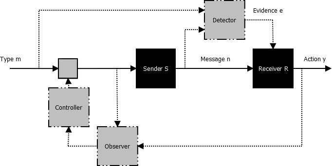
Figure 1.1: A general framework for mechanism design. Manipulating the environment in which deception takes place in a signaling game could include adding additional blocks as well as manipulating exogenous parameters of the game. In general, type $m$ can be manipulated by input from a controller before reaching the sender. The controller can rely on an observer to estimate unknown states. In this paper, we specifically study the roll of a detector, which compares type to message and emits evidence for deception.

In this paper, we study deception in two different frameworks. The first framework is a typical game of costless communication between a sender and receiver known as cheap-talk. In the second framework, we add the element of deception detection, forming a game of cheap-talk with evidence. This latter model includes a move by nature after the action of the sender, which yields evidence for deception with some probability. In order provide a concrete example, we consider a specific use of deception for defense, and the employment of antideceptive techniques by an attacker. In this scenario, a defender uses honeypots disguised as normal systems to protect a network, and an adversary implements honeypot detection in order to strike back against this deception. We give an example of how an adversary might obtain evidence for deception through a timing classification known as fuzzy benchmarking. Finally, we show how network defenders need to bolster their capabilities in order to maintain the same results in the face of honeypot detection. This mechanism design approach reverses the mappings from adversary power to evidence detection and evidence detection to game outcome. Although we apply it to a specific research problem, our approach is quite general and can be used in deceptive interactions in both interpersonal deception and deception in cyber security. Our main contributions include 1) developing a model for signaling games with deception detection, and analyzing how this model includes traditional signaling games and complete information games as special cases, 2) demonstrating that the ability to detect deception causes pure strategy equilibria to disappear under certain conditions, and 3) showing that deception detection by an adversary could actually increase the utility obtained by a network defender. These results have specific implications for network defense through honeypot deployment, but can be applied to a large class of strategic interactions involving deception in both physical and cyberspace.

The rest of the paper proceeds as follows. Section 2 reviews cheap-talk signaling games and the solution concept of perfect Bayesian Nash equilibrium. We use this framework to analyze the honeypot scenario in Section 3. Section 4 adds the element of deception detection to the signaling game. We describe an example of how this detection might be implemented in Section 5. Then we analyze the resulting game in section 6. In Section 7, we discuss a case study in which a network defender needs to change in order to respond to the advent of honeypot detection. We review related work in Section 8, and conclude the paper in Section 9.

2 Cheap-Talk Signaling Games

In this section, we review the concept of signaling games, a class of two-player, dynamic, incomplete information games. The information asymmetry and dynamic nature of these games captures the essence of deception, and the notion of separating, pooling, or partially-separating equilibria can be related to truthful, deceptive, or partially-truthful behavior.

2.1 Game Model

Our model consists of a signaling game in which the types, messages, and actions are taken from discrete sets with two elements. Call this two-player, incomplete information game $\mathcal{G}$. In $\mathcal{G}$, a sender, $S$, observes a type $m\in M=\left\{0,1\right\}$ drawn with probabilities $p\left(0\right)$ and $p\left(1\right)=1-p\left(0\right)$. He then sends a message, $n\in N=\left\{0,1\right\}$ to the receiver, $R$. After observing the message (but not the type), $R$ plays an action $y\in Y=\left\{0,1\right\}$ . The flow of information between sender and receiver is depicted in Fig. 2.1. Let $u^{S}\left(y,m\right)$ and $u^{R}\left(y,m\right)$ be the utility obtained by $S$ and $R$, respectively, when the type is $m$ and the receiver plays action $y$. Notice that the utilities are not directly dependent on the message, $n$; hence the description of this model as a “cheap-talk” game.

Figure 2.1: Block diagram of a signaling game with two discrete types, messages, and actions.

The sender’s strategy consists of playing a message $n$, after observing a type $m$, with probability $\sigma_{S}\left(n\,|\,m\right)$. The receiver’s strategy consists of playing an action $y$, after observing a message $n$, with probability $\sigma_{R}\left(y\,|\,n\right)$. Denote the sets of all such strategies as $\Gamma^{S}$, and $\Gamma^{R}$. Define expected utilities for the sender and receiver as $U^{S}:\,\Gamma^{S}\times\Gamma^{R}\rightarrow\mathbb{R}$ and $U^{R}:\,\Gamma^{S}\times\Gamma^{R}\rightarrow\mathbb{R}$, such that $U^{S}\left(\sigma_{S},\sigma_{R}\right)$ and $U^{R}\left(\sigma_{S},\sigma_{R}\right)$ are the expected utilities for the sender and receiver, respectively, when the sender and receiver play according to the strategy profile $\left(\sigma_{S},\sigma_{R}\right)$. Finally, define $\tilde{U}^{S}:\,\Gamma^{S}\times\Gamma^{R}\times M\to\mathbb{R}$ and $\tilde{U}^{R}:\,\Gamma^{R}\times M\times N\to\mathbb{R}$ such that $\tilde{U}^{S}\left(\sigma_{S},\sigma_{R},m\right)$ gives the expected utility for $S$ for playing $\sigma_{S}$ when $R$ plays $\sigma_{R}$ and the type is $m$, and $\tilde{U}^{R}\left(\sigma_{R},m,n\right)$ gives the expected utility for $R$ for playing $\sigma_{R}$ when the type is $m$ and she observes message $n$.

2.2 Perfect Bayesian Nash Equilibrium

We now review the concept of Perfect Bayesian Nash equilibrium, the natural extension of subgame perfection to games of incomplete information.

A Perfect Bayesian Nash equilibrium (see [11]) of signaling game $\mathcal{G}$ is a strategy profile $\left(\sigma_{S},\sigma_{R}\right)$ and posterior beliefs $\mu_{R}(m\,|\,n)$ of the receiver about the sender such that

$$\forall m\in M,\,\sigma_{S}\in\underset{\bar{\sigma}_{S}\in\Gamma^{S}}{\arg\max\,}\tilde{U}^{S}\left(\bar{\sigma}_{S},\sigma_{R},m\right),$$ (2.1)

$$\forall n\in N,\,\sigma_{R}\in\underset{\bar{\sigma}_{R}\in\Gamma^{R}}{\arg\max}\,\underset{\bar{m}\in M}{\sum}\mu_{R}\left(\bar{m}\,|\,n\right)\tilde{U}^{R}\left(\bar{\sigma}_{R},\bar{m},n\right),$$ (2.2)

$$\mu_{R}\left(m\,|\,n\right)=\begin{cases}\frac{\sigma_{S}\left(n\,|\,m\right)p\left(m\right)}{\underset{\bar{m}\in M}{\sum}\sigma_{S}\left(n\,|\,\bar{m}\right)p\left(\bar{m}\right)},&\text{if}\underset{\bar{m}\in M}{\sum}\sigma_{S}\left(n\,|\,\bar{m}\right)p\left(\bar{m}\right)>0\\ \text{any distrubution on }M,&\text{if}\underset{\bar{m}\in M}{\sum}\sigma_{S}\left(n\,|\,\bar{m}\right)p\left(\bar{m}\right)=0\end{cases}.$$ (2.3)

Eq. 2.1 requires $S$ to maximize his expected utility for the strategy played by $R$ for all types $m$. The second equation requires that, for all messages $n$, $R$ maximizes his expected utility against the strategy played by $S$ given his beliefs. Finally, Eq. 2.3 requires the beliefs of $R$ about the type to be consistent with the strategy played by $S$, using Bayes’ Law to update his prior belief according to $S$’s strategy.

3 Analysis of Deceptive Conflict Using Signaling Games

In this section, we describe an example of deception in cyber security using signaling games. These type of models have been used, for instance, in [12, 13, 14, 15]. We give results here primarily in order to show how the results change after we add the factor of evidence emission in Section 6.

Consider a game $\mathcal{G}_{honey}$, in which a defender uses honeypots to protect a network of computers. We consider a model and parameters from [12], with some adaptations. In this game, the ratio of normal systems to honeypots is considered fixed. Based on this ratio, nature assigns a type - normal system or honeypot - to each system in the network. The sender is the network defender, who can choose to reveal the type of each system or disguise the systems. He can disguise honeypots as normal systems and disguise normal systems as honeypots. The message is thus the network defender’s portrayal of the system. The receiver in this game is the attacker, who observes the defender’s portrayal of the system but not the actual type of the system. He forms a belief about the actual type of the system given the sender’s message, and then chooses an action: attack or withdraw. Table 1 gives the parameters of $\mathcal{G}_{honey}$, and the extensive form of $\mathcal{G}_{honey}$ is given in Fig. 3.1. We have used the game theory software Gambit [16] for this illustration, as well as for simulating the results of games later in the paper.

Table 1: Parameters of $\mathcal{G}_{honey}$. M.S. signifies Mixed Strategy

Parameter Symbol	Meaning
$S$	Network defender
$R$	Network attacker
$m\in\left\{0,1\right\}$	Type of system ($0$: normal; $1$: honeypot)
$n\in\left\{0,1\right\}$	Defender description of system ($0$: normal; $1$: honeypot)
$y\in\left\{0,1\right\}$	Attacker action ($0$: withdraw; $1$: attack)
$p(m)$	Prior probability of type $m$
$\sigma_{S}\left(n\,|\,m\right)$	Sender MS prob. of describing type $m$ as $n$
$\sigma_{R}\left(y\,|\,n\right)$	Receiver MS prob. of action $y$ given description $n$
$v_{o}$	Defender benefit of observing attack on honeypot
$v_{g}$	Defender benefit of avoiding attack on normal system
$-c_{c}$	Defender cost of normal system being compromised
$v_{a}$	Attacker benefit of comprimizing normal system
$-c_{a}$	Attacker cost of attack on any type of system
$-c_{o}$	Attacker additional cost of attacking honeypot

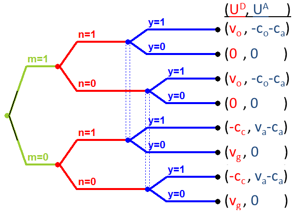
Figure 3.1: Extensive form of $\mathcal{G}_{honey}$, a game in which defender $S$ chooses whether to disguise systems in a network of computers, and an attacker $R$ attempts to gain from compromising normal systems but withdrawing from honeypots. Note that the type $m$ is determined by a chance move.

In order to characterize the equilibria of $\mathcal{G}_{honey}$, define two constants: $\mathcal{CB}_{0}^{R}$ and $\mathcal{CB}_{1}^{S}$. Let $\mathcal{CB}_{0}^{R}$ give the relative benefit to $R$ for playing attack ($y=1$) compared to playing withdraw ($y=0$) when the system is a normal system ($m=0$), and let $\mathcal{CB}_{1}^{R}$ give the relative benefit to $R$ for playing withdraw compared to playing attack when the system is a honeypot ($m=1$). These constants are defined by Eq. 3.1 and Eq. 3.2.

$$\mathcal{CB}_{0}^{R}\triangleq u^{R}\left(1,0\right)-u^{R}\left(0,0\right)$$ (3.1)

$$\mathcal{CB}_{1}^{R}\triangleq u^{R}\left(0,1\right)-u^{R}\left(1,1\right)$$ (3.2)

We now find the pure-strategy separating and pooling equilibria of $\mathcal{G}_{honey}$.

Theorem 1.

The equilibria of $\mathcal{G}_{honey}$ differ in form in three parameter regions:

• Attack-favorable: $p\left(0\right)\mathcal{CB}_{0}^{R}>\left(1-p\left(0\right)\right)\mathcal{CB}_{1}^{R}$

• Defend-favorable: $p\left(0\right)\mathcal{CB}_{0}^{R}<\left(1-p\left(0\right)\right)\mathcal{CB}_{1}^{R}$

• Neither-favorable: $p\left(0\right)\mathcal{CB}_{0}^{R}=\left(1-p\left(0\right)\right)\mathcal{CB}_{1}^{R}$

In attack-favorable, $p\left(0\right)\mathcal{CB}_{0}^{R}>\left(1-p\left(0\right)\right)\mathcal{CB}_{1}^{R}$, meaning loosely that the relative benefit to the receiver for attacking normal systems is greater than the relative loss to the receiver for attacking honeypots. In defend-favorable, $p\left(0\right)\mathcal{CB}_{0}^{R}<\left(1-p\left(0\right)\right)\mathcal{CB}_{1}^{R}$, meaning that the relative loss for attacking honeypots is greater than the relative benefit from attacking normal systems. In neither-favorable, $p\left(0\right)\mathcal{CB}_{0}^{R}=\left(1-p\left(0\right)\right)\mathcal{CB}_{1}^{R}$. We omit analysis of the neither-favorable region because it only arises with exact equality in the game parameters.

3.1 Separating Equilibria

In separating equilibria, the sender plays different pure strategies for each type that he observes. Thus, he completely reveals the truth. The attacker $R$ in $\mathcal{G}_{honey}$ wants to attack normal systems but withdraw from honeypots. The defender $S$ wants the opposite: that the attacker attack honeypots and withdraw from normal systems. Thus, Theorem 2 should come as no surprise.

Theorem 2.

No separating equilibria exist in $\mathcal{G}_{honey}$.

3.2 Pooling Equilibria

In pooling equilibria, the sender plays the same strategies for each type. This is deceptive behavior because the sender’s messages do not convey the type that he observes. The receiver relies only on prior beliefs about the distribution of types in order to choose his action. Theorem 3 gives the pooling equilibria of $\mathcal{G}_{honey}$ in the attack-favorable region.

Theorem 3.

$\mathcal{G}_{honey}$ supports the following pure strategy pooling equilibria in the attack-favorable parameter region:

$$\forall m\in M,\,\sigma_{S}\left(1\,|\,m\right)=1,$$ (3.3)

$$\forall n\in N,\,\sigma_{R}\left(1\,|\,n\right)=1,$$ (3.4)

$$\mu_{R}\left(1\,|\,0\right)\leq\frac{\mathcal{CB}_{0}^{R}}{\mathcal{CB}_{0}^{R}+\mathcal{CB}_{1}^{R}};\;\mu_{R}\left(1\,|\,1\right)=p\left(1\right),$$ (3.5)

and

$$\forall m\in M,\,\sigma_{S}\left(1\,|\,m\right)=0,$$ (3.6)

$$\forall n\in N,\,\sigma_{R}\left(1\,|\,n\right)=1,$$ (3.7)

$$\mu_{R}\left(1\,|\,0\right)=p\left(1\right);\;\mu_{R}\left(1\,|\,1\right)\leq\frac{\mathcal{CB}_{0}^{R}}{\mathcal{CB}_{0}^{R}+\mathcal{CB}_{1}^{R}},$$ (3.8)

both with expected utilities given by

$$U^{S}\left(\sigma_{S},\sigma_{R}\right)=u^{S}\left(1,1\right)-p\left(0\right)\left(u^{S}\left(1,1\right)-u^{S}\left(1,0\right)\right),$$ (3.9)

$$U^{R}\left(\sigma_{S},\sigma_{R}\right)=u^{R}\left(1,1\right)-p\left(0\right)\left(u^{R}\left(1,1\right)-u^{R}\left(1,0\right)\right).$$ (3.10)

Similarly, Theorem 4 gives the pooling equilibria of $\mathcal{G}_{honey}$ in the defend-favorable region.

Theorem 4.

$\mathcal{G}_{honey}$ supports the following pure strategy pooling equilibria in the defend-favorable parameter region:

$$\forall m\in M,\,\sigma_{S}\left(1\,|\,m\right)=1,$$ (3.11)

$$\forall n\in N,\,\sigma_{R}\left(1\,|\,n\right)=0,$$ (3.12)

$$\mu_{R}\left(1\,|\,0\right)\geq\frac{\mathcal{CB}_{0}^{R}}{\mathcal{CB}_{0}^{R}+\mathcal{CB}_{1}^{R}};\;\mu_{R}\left(1\,|\,1\right)=p\left(1\right),$$ (3.13)

and

$$\forall m\in M,\,\sigma_{S}\left(1\,|\,m\right)=0,$$ (3.14)

$$\forall n\in N,\,\sigma_{R}\left(1\,|\,n\right)=0,$$ (3.15)

$$\mu_{R}\left(1\,|\,0\right)=p\left(1\right);\;\mu_{R}\left(1\,|\,1\right)\geq\frac{\mathcal{CB}_{0}^{R}}{\mathcal{CB}_{0}^{R}+\mathcal{CB}_{1}^{R}},$$ (3.16)

both with expected utilities given by

$$U^{S}\left(\sigma_{S},\sigma_{R}\right)=p\left(0\right)\left(u^{S}\left(0,0\right)-u^{S}\left(0,1\right)\right)+u^{S}\left(0,1\right),$$ (3.17)

$$U^{R}\left(\sigma_{S},\sigma_{R}\right)=p\left(0\right)\left(u^{R}\left(0,0\right)-u^{R}\left(0,1\right)\right)+u^{R}\left(0,1\right).$$ (3.18)

In both cases, it is irrelevant whether the defender always sends $1$ or always sends $0$ (always describes systems as honeypots or always describes systems as normal systems); the effect is that the attacker ignores the description. In the attack-favorable region, the attacker always attacks. In the defend-favorable region, the attacker always withdraws.

3.3 Discussion of $\mathcal{G}_{honey}$ Equilibria

We will discuss these equilibria more when we compare them with the equilibria of the game with evidence emission. Still, we note one aspect of the equilibria here. At $p\left(0\right)\mathcal{CB}_{0}^{R}=\left(1-p\left(0\right)\right)\mathcal{CB}_{1}^{R}$, the expected utility is continuous for the receiver, but not for the sender. As shown in Fig. 3.2, the sender’s (network defender’s) utility sharply improves if he transitions from having $p\left(0\right)\mathcal{CB}_{0}^{R}>\left(1-p\left(0\right)\right)\mathcal{CB}_{1}^{R}$ to $p\left(0\right)\mathcal{CB}_{0}^{R}<\left(1-p\left(0\right)\right)\mathcal{CB}_{1}^{R}$, i.e. from having $40\%$ honeypots to having $41\%$ honeypots. This is an obvious mechanism design consideration. We will analyze this case further in the section on mechanism design.

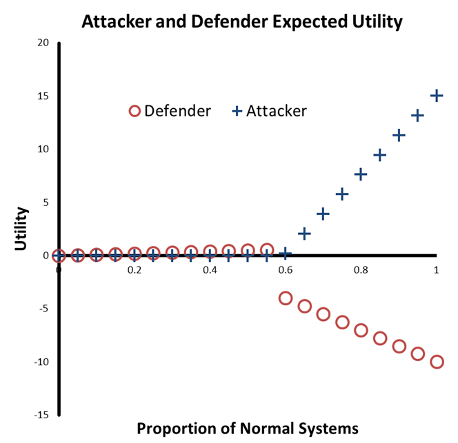
Figure 3.2: Expected Utilities verses Fraction of Normal Systems in Network.

4 Cheap-Talk Signaling Games with Evidence

In Section 3, we used a typical signaling game to model deception in cyberspace (in $\mathcal{G}_{honey}$). In this section, we add to this game the possibility that the sender gives away evidence of deception.

In a standard signaling game, the receiver’s belief about the type is based only on the messages that the sender communicates and his prior belief. In many deceptive interactions, however, there is some probability that the sender gives off evidence of deceptive behavior. In this case, the receiver’s beliefs about the sender’s private information may be updated both based upon the message of the sender and by evidence of deception.

4.1 Game Model

Let $\mathcal{G}^{evidence}$ denote a signaling game with belief updating based both on sender message and on evidence of deception. This game consists of four steps, in which step 3 is new:

1. Sender, $S$, observes type, $m\in M=\left\{0,1\right\}$.

2. $S$ communicates a message, $n\in N=\left\{0,1\right\}$, chosen according to a strategy $\sigma_{S}\left(n\,|\,m\right)\in\Gamma^{S}=\Delta N$ based on the type $m$ that he observes.

3. $S$ emits evidence, $e\in E=\left\{0,1\right\}$ with probability $\lambda\left(e\,|\,m,n\right)$. Signal $e=1$ represents evidence of deception and $e=0$ represents no evidence of deception.

4. Receiver $R$ responds with an action, $y\in Y=\left\{0,1\right\}$, chosen according to a strategy $\sigma_{R}\left(y\,|\,n,e\right)\in\Gamma^{R}=\Delta Y$ based on the message $n$ that he receives and evidence $e$ that he observes.

5. $S$, $R$ receive $u^{S}\left(y,m\right)$, $u^{R}\left(y,m\right)$.

Evidence $e$ is another signal that is available to $R$, in addition to the message $n$. This signal could come, e.g., from a detector, which generates evidence with a probability that is a function of $m$ and $n$. The detector implements the function $\lambda\left(e\,|\,m,n\right)$. We depict this view of the signaling game with evidence emission in Fig. 4.1. We assume that $\lambda\left(e\,|\,m,n\right)$ is common knowledge to both the sender and receiver. Since evidence is emitted with some probability, we model this as a move by a “chance” player, just as we model the random selection of the type at the beginning of the game as a move by a chance player. The outcome of the new chance move will be used by $R$ together with his observation of $S$’s action to formulate his belief about the type $m$. We describe this belief updating in the next section.

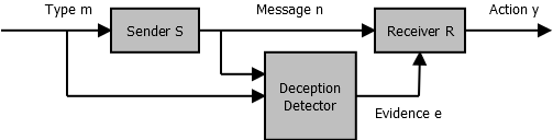
Figure 4.1: Block diagram of a signaling game with evidence emission.

4.2 Two-step Bayesian Updating

Bayesian updating is a two-step process, in which the receiver first updates his belief about the type based on the observed message of the sender, and then updates his belief a second time based on the evidence emitted. The following steps formulate the update process.

1. $R$ observes $S$’s action. He computes belief $\mu_{R}\left(m\,|\,n\right)$ based on the prior likelihoods $p\left(m\right)$ of each type and $S$’s message $n$ according to Eq. 2.3, which we rewrite here in Eq. 4.1.

   $$\mu_{R}\left(m\,|\,n\right)=\begin{cases}\frac{\sigma_{S}\left(n\,|\,m\right)p\left(m\right)}{\underset{\bar{m}\in M}{\sum}\sigma_{S}\left(n\,|\,\bar{m}\right)p\left(\bar{m}\right)},&\text{if}\underset{\bar{m}\in M}{\sum}\sigma_{S}\left(n\,|\,\bar{m}\right)p\left(\bar{m}\right)>0\\ \text{any distribution on }M,&\text{if}\underset{\bar{m}\in M}{\sum}\sigma_{S}\left(n\,|\,\bar{m}\right)p\left(\bar{m}\right)=0\end{cases}$$ (4.1)

2. $S$ computes a new belief based on the evidence emitted. The prior belief in this second step is given by $\mu_{R}\left(m\,|\,n\right)$ obtained in the first step. The conditional probability of emitting evidence $e$ when the type is $m$ and the sender communicates message $n$ is $\lambda\left(e\,|\,m,n\right)$. Thus, the receiver updates his belief in this second step according to

   $$\mu_{R}\left(m\,|\,n,e\right)=\begin{cases}\frac{\lambda\left(e\,|\,m,n\right)\mu_{R}\left(m\,|\,n\right)}{\underset{\bar{m}\in M}{\sum}\lambda\left(e\,|\,\bar{m},n\right)\mu_{R}\left(\bar{m}\,|\,n\right)},&\text{if}\underset{\bar{m}\in M}{\sum}\lambda\left(e\,|\,\bar{m},n\right)\mu_{R}\left(\bar{m}\,|\,n\right)>0\\ \text{any distribution on }M,&\text{if}\underset{\bar{m}\in M}{\sum}\lambda\left(e\,|\,\bar{m},n\right)\mu_{R}\left(\bar{m}\,|\,n\right)=0\end{cases}.$$ (4.2)

Having formulated the belief updating rules, we now give the conditions for a Perfect Bayesian Nash equilibrium in our signaling game with evidence emission.

4.3 Perfect Bayesian Nash Equilibrium in Signaling Game with Evidence

The conditions for a Perfect Bayesian Nash Equilibrium of our augmented game are the same as those for the original signaling game, except that the belief update includes the use of emitted evidence. Here, however, we must also define a new utility function for $R$ that takes expectation conditional upon $e$ in addition to $n$. Define this utility function by $\hat{U}^{R}:\,\Gamma^{R}\times M\times N\times E\to\mathbb{R}$ such that $\hat{U}^{R}\left(\sigma_{R},m,n,e\right)$ gives the expected utility for $R$ for playing $\sigma_{R}$ when the type is $m$ and she observes message $n$ and evidence $e$.

Definition 1.

A perfect Bayesian Nash equilibrium of the game $\mathcal{G}^{evidence}$ is a strategy profile $\left(\sigma_{S},\sigma_{R}\right)$ and posterior beliefs $\mu_{R}(m\,|\,n,e)$, such that system given by Eq. 4.3 through Eq. 4.6 are simultaneously satisfied.

$$\forall m\in M,\,\sigma_{S}\in\underset{\bar{\sigma}_{S}\in\Gamma^{S}}{\arg\max\,}\tilde{U}^{S}\left(\bar{\sigma}_{S},\sigma_{R},m\right)$$ (4.3)

$$\forall n\in N,\,\forall e\in E,\,\sigma_{R}\in\underset{\bar{\sigma}_{R}\in\Gamma^{R}}{\arg\max\,}\underset{\bar{m}\in M}{\sum}\mu_{R}(\bar{m}\,|\,n,e)\hat{U}^{R}\left(\bar{\sigma}_{R},\bar{m},n,e\right)$$ (4.4)

$$\forall n\in N,\,\mu_{R}\left(m\,|\,n\right)=\begin{cases}\frac{\sigma_{S}\left(n\,|\,m\right)p\left(m\right)}{\underset{\bar{m}\in M}{\sum}\sigma_{S}\left(n\,|\,\bar{m}\right)p\left(\bar{m}\right)},&\text{if}\underset{\bar{m}\in M}{\sum}\sigma_{S}\left(n\,|\,\bar{m}\right)p\left(\bar{m}\right)>0\\ \text{any distribution on }M,&\text{if}\underset{\bar{m}\in M}{\sum}\sigma_{S}\left(n\,|\,\bar{m}\right)p\left(\bar{m}\right)=0\end{cases}$$ (4.5)

$$\begin{array}[]{c}\forall n\in N,\,\forall e\in E,\\ \mu_{R}\left(m\,|\,n,e\right)=\end{array}\begin{cases}\frac{\lambda\left(e\,|\,m,n\right)\mu_{R}\left(m\,|\,n\right)}{\underset{\bar{m}\in M}{\sum}\lambda\left(e\,|\,\bar{m},n\right)\mu_{R}\left(\bar{m}\,|\,n\right)},&\text{if}\underset{\bar{m}\in M}{\sum}\lambda\left(e\,|\,\bar{m},n\right)\mu_{R}\left(\bar{m}\,|\,n\right)>0\\ \text{any distribution on }M,&\text{if}\underset{\bar{m}\in M}{\sum}\lambda\left(e\,|\,\bar{m},n\right)\mu_{R}\left(\bar{m}\,|\,n\right)=0\end{cases}$$ (4.6)

Again, the first two definitions require the sender and receiver to maximize their expected utilities. The third and fourth equations require belief consistency in terms of Bayes’ Law.

5 Deception Detection Example in Network Defense

Consider again our example of deception in cyberspace in which a defender protects a network of computer systems using honeypots. The defender has the ability to disguise normal systems as honeypots and honeypots as normal systems. In Section 3, we modeled this deception as if it were possible for the defender to disguise the systems without any evidence of deception. In reality, attackers may try to detect honeypots. For example, send-safe.com’s “Honeypot Hunter” [17] checks lists of HTTPS and SOCKS proxies and outputs text files of valid proxies, failed proxies, and honeypots. It performs a set of tests which include opening a false mail server on the local system to test the proxy connection, connecting to the proxy port, and attempting to proxy back to its false mail server [18].

Another approach to detecting honeypots is based on timing. [19] used a process termed fuzzy benchmarking in order to classify systems as real machines or virtual machines, which could be used e.g., as honeypots. In this process, the authors run a set of instructions which yield different timing results on different host hardware architectures in order to learn more about the hardware of the host system. Then, they run a loop of control modifying CPU instructions (read and write control register 3, which induces a translation lookaside buffer flush) that results in increased run-time on a virtual machine compared to a real machine. The degree to which the run-times are different between the real and virtual machines depends on the number of sensitive instructions in the loop. The goal is to run enough sensitive instructions to make the divergence in run-time - even in the presence of internet noise - large enough to reliably classify the system using a timing threshold. They do not identify limits to the number of sensitive instructions to run, but we can imagine that the honeypot detector might itself want to go undetected by the honeypot and so might want to limit the number of instructions.

Although they do not recount the statistical details, such an approach could result in a classification problem which can only be accomplished successfully with some probability. In Fig. 5.1, $t$ represents the execution time of the fuzzy benchmarking code. The curve $f_{0}\left(t\right)$ represents the probability density function for execution time for normal systems ($m=0$), and the curve $f_{1}\left(t\right)$ represents the probability density function for execution time for virtual machines ($m=1$). The execution time $t_{d}$ represents a threshold time used to classify the system under test. Let $AR_{i}$, $i\in\left\{1,2,3,4\right\}$ denote the area under regions $R_{1}$ through $R_{4}$. We have defined $\lambda\left(e\,|\,m,n\right)$ to be the likelihood with which a system of type $m$ represented as a system as type $n$ gives off evidence for deception $e$ (where $e=1$ represents evidence for deception and $e=0$ represents evidence for truth-telling). A virtual machine disguised as a normal system may give off evidence for deception, in this case in terms of the run-time of fuzzy benchmarking code. We would then have that

$$\begin{array}[]{c}\lambda\left(1\,|\,1,0\right)=AR_{3}+AR_{4}\\ \lambda\left(0\,|\,1,0\right)=AR_{2}=1-\left(AR_{3}+AR_{4}\right)\end{array}.$$ (5.1)

If the system under test were actually a normal system, then the same test could result in some likelihood of a false-positive result for deception. Then, we would have

$$\begin{array}[]{c}\lambda\left(1\,|\,0,0\right)=AR_{3}\\ \lambda\left(0\,|\,0,0\right)=AR_{1}+AR_{2}=1-\left(AR_{3}\right)\end{array}.$$ (5.2)

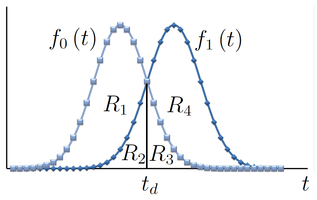
Figure 5.1: Classification of systems as normal or virtual (e.g. a honeypot) based on run-time for a set of control modifying CPU instructions (based on fuzzy benchmarking in [19]).

Let us assume that the likelihood with which one type of system masquerading as another can be successfully detected is the same regardless of whether it is a honeypot that is disguised as a normal system or it is a normal system that is disguised as a honeypot. Denote this probability as $\epsilon\in\left[0,1\right]$. Let $\delta\in\left[0,1\right]$ be defined as the likelihood of falsely detecting deception. These probabilities are given by

$$\epsilon=\lambda\left(1\,|\,m,n\right),\,m\neq n,$$ (5.3)

$$\delta=\lambda\left(1\,|\,m,n\right)\,m=n.$$ (5.4)

In [19], the authors tune the number of instructions for the CPU to run in order to sufficiently differentiate normal systems and honeypots. In this case, $\epsilon$ and $\delta$ may relate to the number of instructions that the detector asks the CPU to run. In general, though, the factors which influence $\epsilon$ and $\delta$ could vary. Powerful attackers will have relatively high $\epsilon$ and low $\delta$ compared to less powerful attackers. Next, we study this network defense example using our model of signaling games with evidence.

6 Analysis of Network Defense using Signaling Games with Evidence

Figure 6.1 depicts an extensive-form of the signaling game with evidence for our network defense problem. Call this game $\mathcal{G}_{honey}^{evidence}$. (See [12] for a more detailed explanation of the meaning of the parameters.) In the extremes of $\epsilon$ and $\delta$, we will see that the game degenerates into simpler types of games.

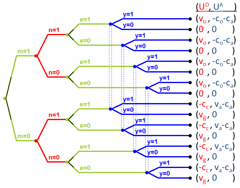
Figure 6.1: Extensive form depiction of $\mathcal{G}_{honey}^{evidence}$. Note that the type $m$ and the evidence $e$ are both determined by chance moves.

First, because $R$ updates his belief based on evidence emission in a Bayesian manner, any situation in which $\delta=\epsilon$ will render the evidence useless. The condition $\delta=\epsilon$ would arise from an attacker completely powerless to detect deception. This is indicated in Fig. 6.2 by the region game without evidence, which we term $\mathcal{R}_{Weak}$ to indicate an attacker with weak detection capability.

Second, on the other extreme, we have the condition $\epsilon=1,\,\delta=0$, which indicates that the attacker can always detect deception and never registers false positives. Denote this region $\mathcal{R}_{Omnipotent}$ to indicate an attacker with omnipotent detection capability. $\mathcal{R}_{Omnipotent}$ degenerates into a complete information game in which both $S$ and $R$ are able to observe the type $m$.

Third, we have a condition in which the attacker’s detection capability is such that evidence guarantees deception (when $\delta=0$ but $\epsilon$ is not necessarily $1$) and a condition in which the attacker’s power is such that no evidence guarantees truth-telling (when $\epsilon=1$ but $\delta$ is not necessarily $0$). We can term these two regions $\mathcal{R}_{Conservative}$ and $\mathcal{R}_{Aggressive}$, because the attacker never detects a false positive in $\mathcal{R}_{Conservative}$ and never misses a sign for deception in $\mathcal{R}_{Aggressive}$.

Finally, we have the region $\mathcal{R}_{Intermediate}$ in which the attacker’s detection capability is powerful enough that he correctly detects deception with greater rate than he registers false positives, but does not achieve $\delta=0$ or $\epsilon=1$. We list these attacker conditions in Table 2. Let us examine the equilibria of $\mathcal{G}_{honey}^{evidence}$ in these different cases.

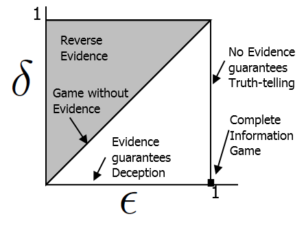
Figure 6.2: Degenerate cases of $\mathcal{G}_{honey}^{evidence}$

Table 2: Attacker capabilities for degenerate cases of $\mathcal{G}_{honey}^{evidence}$

Name of Region	Description of Region	Parameter Values
$\mathcal{R}_{Weak}$	Game without evidence	$\delta=\epsilon$
$\mathcal{R}_{Omnipotent}$	Complete information game	$\epsilon=1,\,\delta=0$
$\mathcal{R}_{Conservative}$	Evidence guarantees deception	$\delta=0$
$\mathcal{R}_{Aggressive}$	No evidence guarantees truth-telling	$\epsilon=1$
$\mathcal{R}_{Intermediate}$	No guarantees	$\epsilon\neq 1>\delta\neq 0$

6.1 Equilibria for $\mathcal{R}_{Weak}$

The equilibria for $\mathcal{R}_{Weak}$ are given by our analysis of the game without evidence ($\mathcal{G}_{honey}$) in Section 3. Recall that a separating equilibrium was not sustainable, while pooling equilibria did exist. Also, the equilibrium solutions fell into two different parameter regions. The sender’s utility was discontinuous at the interface between parameter regions, creating an optimal proportion of normal systems that could be included in a network while still deterring attacks.

6.2 Equilibria for $\mathcal{R}_{Omnipotent}$

For $\mathcal{R}_{Omnipotent}$, the attacker knows with certainty the type of system (normal or honeypot) that he is facing. If the evidence indicates that the system is a normal system, then he attacks. If the evidence indicates that the system is a honeypot, then he withdraws. The defender’s description is unable to disguise the type of the system. Theorem 5 gives the equilibrium strategies and utilities.

Theorem 5.

$\mathcal{G}_{honey}^{evidence}$, under adversary capabilities $\mathcal{R}_{Omnipotent}$ supports the following equilibria:

$$\sigma_{S}\left(m\,|\,n\right)\in\Gamma^{S}$$ (6.1)

$$\sigma_{R}\left(1\,|\,n,e\right)=\begin{cases}n,&e=1\\ 1-n,&e=0\end{cases},\,\forall n\in N,$$ (6.2)

$$\mu_{R}\left(1\,|\,n,e\right)=\begin{cases}1-n,&e=1\\ n,&e=0\end{cases},\,\forall n\in N,$$ (6.3)

with expected utilities given by

$$U^{S}\left(\sigma_{S},\sigma_{R}\right)=p\left(0\right)\left(u^{S}\left(1,0\right)-u^{S}\left(0,1\right)\right)+u^{S}\left(0,1\right),$$ (6.4)

$$U^{R}\left(\sigma_{S},\sigma_{R}\right)=p\left(0\right)\left(u^{R}\left(1,0\right)-u^{R}\left(0,1\right)\right)+u^{R}\left(0,1\right).$$ (6.5)

Similarly to $\mathcal{R}_{Weak}$, in $\mathcal{R}_{Omnipotent}$ the expected utilities for $S$ and $R$ are the same regardless of the equilibrium strategy chosen (although the equilibrium strategy profiles are not as interesting here because of the singular role of evidence).

Next, we analyze the equilibria in the non-degenerate cases, $\mathcal{R}_{Conservative}$, $\mathcal{R}_{Aggressive}$, and $\mathcal{R}_{Intermediate}$ , by numerically solving for equilibria under selected parameter settings.

6.3 Equilibria for $\mathcal{R}_{Conservative}$ , $\mathcal{R}_{Aggressive}$, and $\mathcal{R}_{Intermediate}$

In Section 3, we found analytical solutions for the equilibria of a signaling game in which the receiver does not have the capability to detect deception. In this section, we give results concerning signaling games in which the receiver does have the capability to detect deception, using illustrative examples rather than an analytical solution. To study equilibria under the three non-degenerate cases, we choose a set of parameters for the attacker and defender utilities (Table 3). In this model (from [12]), the defender gains utility from maintaining normal systems that are not attacked in the network, and also from observing attacks on honeypots. The defender incurs a loss if a normal system is attacked. The attacker, on the other hand, gains only from attacking a normal system; he incurs losses if he attacks a honeypot.

Table 3: Sample parameters which describe $\mathcal{GS}_{honey}^{evidence}$

Parameter Symbol	Value
$v_{o}$, sender utility from observing attack on honeypot	$5$
$v_{g}$, sender utility from normal system surviving	$1$
$-c_{C}$, sender cost for compromised normal system	$-10$
$-c_{o}-c_{a}$, cost due to attacker for attacking honeypot	$-22$
$0$, utility for attacker for withdrawing from any system	$0$
$v_{a}-c_{a}$, benefit of attacker for compromising normal system	$15$

Based on these parameters, we can find the equilibrium utilities at each terminal node of Fig. 6.1. We study examples in the attacker capability regions of $\mathcal{R}_{Conservative}$ , $\mathcal{R}_{Aggressive}$, and $\mathcal{R}_{Intermediate}$. For each of these attacker capabilities, we look for equilibria in pure strategies under three different selected values for the percentage of normal systems (compared to honeypots) that make up a network. For the high case, we set the ratio of normal systems to total systems to be $p\left(0\right)=0.9$. Denote this case normal-saturated. For the medium case, we set $p\left(0\right)=0.6$. Denote this case non-saturated. Finally, label the low case, in which $p\left(0\right)=0.2$, honeypot-saturated. For comparison, we also include the equilibria under the same game with no evidence emission (which corresponds to $\mathcal{R}_{Weak}$ ), and the equilibria under the same game with evidence that has a true-positive rate of $1.0$ and a false-positive rate of $0$ (which corresponds to $\mathcal{R}_{Omnipotent}$ ). In Table 4, we list whether each parameter set yields pure strategy equilibria.

Table 4: Equilibria for Selected Parameter Values in $\mathcal{R}_{Conservative}$ , $\mathcal{R}_{Aggressive}$, and $\mathcal{R}_{Intermediate}$ , when the percentage of honeypots in a network is high, medium, and low.

Saturation	$\mathcal{R}_{Weak}$	$\mathcal{R}_{Intermediate}$, $\mathcal{R}_{Conservative}$, $\mathcal{R}_{Aggressive}$	$\mathcal{R}_{Omnipotent}$
Normal	Yes	Yes	Yes
None	Yes	None	Yes
Honeypot	Yes	Yes	Yes

For adversary detection capabilities represented by $\mathcal{R}_{Weak}$ , we have a standard signaling game, and thus the well-known result that a (pooling) equilibrium always exists. In $\mathcal{R}_{Omnipotent}$, the deception detection is fool-proof, and thus the receiver knows the type with certainty. We are left with a complete information game. Essentially, the type merely determines which Stackelberg game the sender and receiver play. Because pure strategy equilibria always exist in Stackelberg games, $\mathcal{R}_{Omnipotent}$ also always has pure-strategy equilibria. The rather unintuitive result comes from $\mathcal{R}_{Intermediate}$, $\mathcal{R}_{Conservative}$, and $\mathcal{R}_{Aggressive}$. In these ranges, the receiver’s ability to detect deception falls somewhere between no capability ($\mathcal{R}_{Weak}$ ) and perfect capability ($\mathcal{R}_{Omnipotent}$ ). Those regions exhibit pure-strategy equilibria, but the intermediate regions may not. Specifically, they appear to fail to support pure-strategy equilibria when the ratio of honeypots within the network does not fall close to either $1$ or $0$. In Section 7 on mechanism design, we will see that this region plays an important role in the comparison of network defense - and deceptive interactions in general - with and without the technology for detecting deception.

7 Mechanism Design for Detecting or Leveraging Deception

In this section, we discuss design considerations for a defender who is protecting a network of computers using honeypots. In order to do this, we choose a particular case study, and analyze how the network defender can best set parameters to achieve his goals. We also discuss the scenario from the point of view of the attacker. Specifically, we examine how the defender can set the exogenous properties of the interaction in 1) the case in which honeypots cannot be detected, and 2) the case in which the attacker has implemented a method for detecting honeypots. Then, we discuss the difference between these two situations.

7.1 Attacker Incapable of Honeypot Detection

First, consider the case in which the attacker does not have the ability to detect honeypots, i.e. $\mathcal{G}_{honey}$. The parameters which determine the attacker and defender utilities are set according to Table 3. The attacker’s utility as a function of the fraction of normal systems in the network is given by the red (circular) data points in Fig. 7.2. We can distinguish two parameter regions. When the proportion of honeypots in the network is greater than approximately $40\%$, (i.e. $p\left(0\right)<60\%$), the attacker is completely deterred. Because of the high likelihood that he will encounter a honeypot if he attacks, he chooses to withdraw from all systems. As the proportion of normal systems increases after $p\left(0\right)>60\%$, he switches to attacking all systems. He attacks regardless of the sender’s signal, because in the pooling equilibrium, his signal does not convey any information about the type to the receiver. In this domain, as the proportion of normal systems increases, the expected utility of the attacker increases.

For this case in which the attacker cannot detect honeypots, the defender’s expected utility as a function of $p\left(0\right)$ is given by the red (circular) data points in Fig. 7.2. We have noted that, in the domain $p\left(0\right)<60\%$, the attacker always withdraws. In this domain, it is actually beneficial for the defender to have as close as possible to the transition density of $60\%$ normal systems, because he gains more utility from normal systems that are not attacked than from honeypots that are not attacked. But if the defender increases the proportion of normal systems beyond $60\%$, he incurs a sudden drop in utility, because the attacker switches form never attacking to always attacking. Thus, the if the defender has the capability to design his network with any number of honeypots, he faces an optimization in which he wants to have as close as possible to $40\%$ of systems be normal .

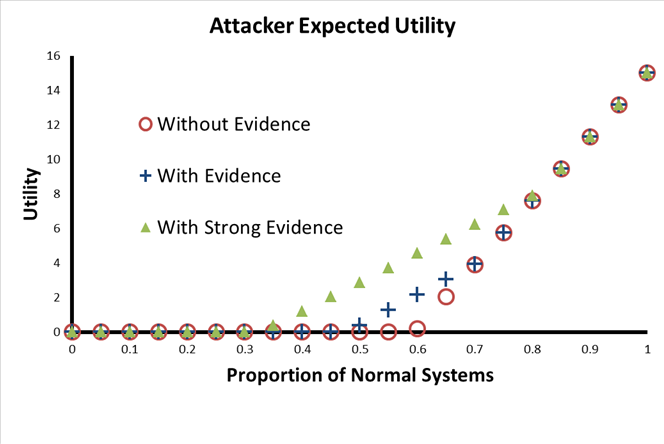
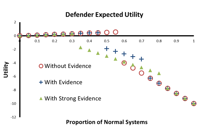
Figure 7.1: Expected utility for the attacker in games of $\mathcal{G}_{honey}$ and $\mathcal{G}_{honey}^{evidence}$ as a function of the fraction $p\left(0\right)$ of normal systems in the network.

Figure 7.2: Expected utility for the defender in games of $\mathcal{G}_{honey}$ and $\mathcal{G}_{honey}^{evidence}$ as a function of the fraction $p\left(0\right)$ of normal systems in the network.

7.2 Attacker Capable of Honeypot Detection

Consider now how the network defense is affected if the attacker gains some ability to detect deception. This game takes the form of $\mathcal{G}_{honey}^{evidence}$. Recall that, in this form, a chance move has been added after the sender’s action. The chance move determines whether the receiver observes evidence that the sender is being deceptive. For Fig. 7.2 and Fig. 7.2, we have set the detection rates at $\epsilon=0.8$ and $\delta=0.5$. These fall within the attacker capability range $\mathcal{R}_{intermediate}$. Observing evidence does not guarantee deception; neither does a lack of evidence guarantee truth-revelation.

In the blue (cross) data points in Fig. 7.2, we see that, at the extremes of $p\left(0\right)$, the utility of the attacker is unaffected by the ability to detect deception according to probabilities $\epsilon$ and $\delta$. The low ranges of $p\left(0\right)$, as described in table 4, correspond to the honeypot-saturated region. In this region, honeypots predominate to such an extent that the attacker is completely deterred from attacking. Note that, compared to the data points for the case without deception detection, the minimum proportion of honeypots which incentives the attacker to uniformly withdraw has increased. Thus, for instance, a $p\left(0\right)$ of approximately $0.50$ incentivizes an attacker without deception detection capabilities to withdraw from all systems, but does not incentivize an attacker with deception detection capabilities to withdraw. At $p\left(0\right)=0.50$, the advent of honeypot-detection abilities causes the defender’s utility to drop from $0.5$ to approximately $-2$. At the other end of the $p\left(0\right)$ axis, we see that a high-enough $p\left(0\right)$ causes the utilities to again be unaffected by the ability to detect deception. This is because the proportion of normal systems is so high that the receiver’s best strategy is to attack constantly (regardless of whether he observes evidence for deception).

In the middle (non-saturated) region of $p\left(0\right)$, the attacker’s strategy is no longer to solely attack or solely withdraw. This causes the “cutting the corner” behavior of the attacker’s utility in Fig. 7.2. This conditional strategy also induces the middle region for the defender’s utility in Fig. 7.2. Intuitively, we might expect that the attacker’s ability to detect deception could only decrease the defender’s utility. But the middle (non-saturated) range of $p\left(0\right)$ shows that this is not the case. Indeed from approximately $p\left(0\right)=0.6$ to $p\left(0\right)=0.7$, the defender actually benefits from the attacker’s ability to detect deception! The attacker, himself, always benefits from the ability to detect deception. Thus, there is an interesting region of $p\left(0\right)$ for which the ability of the attacker to detect deception results in a mutual benefit.

Finally, we can examine the effect of evidence as it becomes more powerful in the green (triangle) points in Fig. 7.2 and Fig. 7.2. These equilibria were obtained for $\epsilon=0.9$ and $\delta=0.3$. This more powerful detection capability broadens the middle parameter domain in which the attacker bases his strategy partly upon evidence. Indeed, in the omnipotent detector case, the plots for both attacker and defender consist of straight lines from their utilities at $p\left(0\right)=0$ to their utilities at $p\left(0\right)=1$. Because the attacker with omnipotent detector is able to discern the type of the system completely, his utility grows in proportion with the proportion of normal systems, which he uniformly attacks. He withdraws uniformly from honeypots.

8 Related Work

Deception has become a critical research area, and several works have studied problems similar to ours. Alcan et al. [13] discuss how to combine sensing technologies within a network with game theory in order to design intrusion detection systems. They study two models. The first is a cooperative game, in which the contribution of different sensors towards detecting an intrusion determines the coalitions of sensors whose threat values will be used in computing the threat level. In the second model, they include the attacker, who determines which subsystems to attack. This model is a dynamic (imperfect) information game, meaning that as moves place the game in various information sets, players learn about the history of moves. Unlike our model, it is a complete information game, meaning that both players know the utility functions of the other player.

Farhang et al. study a multiple-period, information-asymmetric attacker-defender game involving deception [14]. In their model, the sender type - benign or malicious - is known only with an initial probability to the receiver, and that probability is updated in a Bayesian manner during the course of multiple interactions. In [15], Zhuang et al. study deception in multiple-period signaling games, but their paper also involves resource-allocation. The paper has interesting insights into the advantage to a defender of maintaining secrecy. Similar to our work, they consider an example of defensive use of deception. In both [14] and [15], however, players update beliefs only through repeated interactions, whereas one of the players in our model incorporates a mechanism for deception detection.

We have drawn most extensively from the work of Carroll and Grosu [12], who study the strategic use of honeypots for network defense in a signaling game. The parameters of our attacker and defender utilities come from [12], and the basic structure of our signaling game is adapted from that work. In [12], the type of a particular system is chosen randomly from the distribution of normal systems and honeypots. Then the sender chooses how to describe the system (as a normal system or as a honeypot), which may be truthful or deceptive. For the receiver’s move, he may choose to attack, to withdraw, or to condition his attack on testing the system. In this way, honeypot detection is included in the model. Honeypot detection adds a cost to the attacker regardless of whether the system being tested is a normal system or a honeypot, but mitigates the cost of an attack being observed in the case that the system is a honeypot. In our paper, we enrich the representation of honeypot testing by making its effect on utility endogenous. We model the outcome of this testing as an additional move by nature after the sender’s move. This models detection as technique which may not always succeed, and to which both the sender and receiver can adapt their equilibrium strategies.

9 Discussion

In this paper, we have investigated the ways in which the outcomes of a strategic, deceptive interaction are affected by the advent of deception-detecting technology. We have studied this problem using a version of a signaling game in which deception may be detected with some probability. We have modeled the detection of deception as a chance move that occurs after the sender selects a message based on the type that he observes. For the cases in which evidence is trivial or omnipotent, we have given the analytical equilibrium outcome, and for cases in which evidence has partial power, we have presented numerical results. Throughout the paper, we have used the example of honeypot implementation in network defense. In this context, the technology of detecting honeypots has played the role of a malicious use of anti-deception. This has served as a general example to show how equilibrium utilities and strategies can change in games involving deception when the agent being deceived gains some detection ability.

Our first contribution is the model we have presented for signaling games with deception detection. We also show how special cases of this model cause the game to degenerate into a traditional signaling game or into a complete information game. Our model is quite general, and could easily be applied to strategic interactions in interpersonal deception such as border control, international negotiation, advertising and sales, and suspect interviewing. Our second contribution is the numerical demonstration showing that pure-strategy equilibria are not supported under this model when the distribution of types is in a middle range but are supported when the distribution is close to either extreme. Finally, we show that it is possible that the ability of a receiver to detect deception could actually increase the utility of a possibly-deceptive sender. These results have concrete implications for network defense through honeypot deployment. More importantly, they are also general enough to apply to the large and critical body of strategic interactions that involve deception.

References

- [1] R. Dawkins, The Selfish Gene. Oxford University Press, 1976.
- [2] W. von Hippel and R. Trivers, “The evolution and psychology of self-deception,” Behavioral and Brain Sciences, vol. 34, no. 01, pp. 1–16, Feb. 2011.
- [3] A. Vrij, S. A. Mann, R. P. Fisher, S. Leal, and R. Milne, “Increasing cognitive load to facilitate lie detection: The benefit of recalling an event in reverse order,” Law and Human Behavior, vol. 32, no. 3, pp. 253–265, Jun. 2008.
- [4] C. F. Bond and B. M. DePaulo, “Individual differences in judging deception: Accuracy and bias.,” Psychological Bulletin, vol. 134, no. 4, pp. 477–492, 2008.
- [5] J. M. Vendemia, R. F. Buzan, and E. P. Green, “Practice effects, workload, and reaction time in deception,” The American Journal of Psychology, pp. 413–429, 2005.
- [6] S. A. Mann, S. A. Leal, and R. P. Fisher, “‘Look into my eyes’: can an instruction to maintain eye contact facilitate lie detection?” Psychology, Crime and Law, vol. 16, no. 4, pp. 327–348, 2010.
- [7] A. Vrij and P. A. Granhag, “Eliciting cues to deception and truth: What matters are the questions asked,” Journal of Applied Research in Memory and Cognition, vol. 1, no. 2, pp. 110–117, Jun. 2012.
- [8] Cyber War and Cyber Terrorism, ed. A. Colarik and L. Janczewski, Hershey, PA: The Idea Group, 2007.
- [9] M. Ott, Y. Choi, C. Cardie, and J. T. Hancock, “Finding deceptive opinion spam by any stretch of the imagination,” in Proceedings of the 49th Annual Meeting of the Association for Computational Linguistics: Human Language Technologies, Volume 1, 2011, pp. 309–319.
- [10] J. T. Wang, M. Spezio, and C. F. Camerer, “Pinocchio’s Pupil: Using Eyetracking and Pupil Dilation to Understand Truth Telling and Deception in Sender-Receiver Games,” The American Economic Review, vol. 100, no. 3, pp. 984–1007, Jun. 2010.
- [11] D. Fudenberg, and J. Tirole, Game Theory. Cambridge, MA: MIT Press, 1991.
- [12] T. E. Carroll and D. Grosu, “A game theoretic investigation of deception in network security,” Security and Communication Networks, vol. 4, no. 10, pp. 1162–1172, 2011.
- [13] T. Alpcan, and T. Başar, “A game theoretic approach to decision and analysis in network intrusion detection,” in Proceedings of the 42nd IEEE Conference on Decision and Control, 2003.
- [14] S. Farhang, M. H. Manshaei, M. N. Esfahani, and Q. Zhu, “A Dynamic Bayesian Security Game Framework for Strategic Defense Mechanism Design,” Decision and Game Theory for Security, pp. 319–328, 2014.
- [15] J. Zhuang, V. M. Bier, and O. Alagoz, “Modeling secrecy and deception in a multiple-period attacker–defender signaling game,” European Journal of Operational Research, vol. 203, no. 2, pp. 409–418, Jun. 2010.
- [16] R. D. McKelvey, A. M. McLennan, and T. L. Turocy. Gambit: Software Tools for Game Theory, Version 14.1.0. http://www.gambit-project.org. 2014.
- [17] “Send-Safe Honeypot Hunter - honeypot detecting software.” [Online]. Available: http://www.send-safe.com/honeypot-hunter.html. [Accessed: 23-Feb-2015].
- [18] N. Krawetz, “Anti-honeypot technology,” Security & Privacy, IEEE, vol. 2, no. 1, pp. 76–79, 2004.
- [19] J. Franklin, M. Luk, J. M. McCune, A. Seshadri, A. Perrig, and L. Van Doorn, “Remote detection of virtual machine monitors with fuzzy benchmarking,” ACM SIGOPS Operating Systems Review, vol. 42, no. 3, pp. 83–92, 2008.