Dictionary learning with few samples and matrix concentration

Abstract.

Let $A$ be an $n\times n$ matrix, $X$ be an $n\times p$ matrix and $Y=AX$. A challenging and important problem in data analysis, motivated by dictionary learning and other practical problems, is to recover both $A$ and $X$, given $Y$. Under normal circumstances, it is clear that this problem is underdetermined. However, in the case when $X$ is sparse and random, Spielman, Wang and Wright showed that one can recover both $A$ and $X$ efficiently from $Y$ with high probability, given that $p$ (the number of samples) is sufficiently large. Their method works for $p\geq Cn^{2}\log^{2}n$ and they conjectured that $p\geq Cn\log n$ suffices. The bound $n\log n$ is sharp for an obvious information theoretical reason.

In this paper, we show that $p\geq Cn\log^{4}n$ suffices, matching the conjectural bound up to a polylogarithmic factor. The core of our proof is a theorem concerning $l_{1}$ concentration of random matrices, which is of independent interest.

Our proof of the concentration result is based on two ideas. The first is an economical way to apply the union bound. The second is a refined version of Bernstein’s concentration inequality for the sum of independent variables. Both have nothing to do with random matrices and are applicable in general settings.

1. Introduction

Let $A$ be an $n\times n$ invertible matrix and $X$ be an $n\times p$ matrix; set $Y:=AX$. The aim of this paper is to study the following recovery problem:

Given $Y$, reconstruct $A$ and $X$.

It is clear that in the equation

(1.1) $$Y=AX,$$

we have $n^{2}+np$ unknowns (the entries of $A$ and $X$), and only $np$ equations (given by the entries of $Y$). Thus, the problem is underdetermined and one cannot hope for a unique solution. However, in practice, $X$ is frequently a sparse matrix. If $X$ is sparse, the number of unknowns decreases dramatically, as the majority of entries of $X$ are zero. The name of the game here is to find the minimum value of $p$, the number of observations, which guarantees a unique recovery (e.g. [2] and [6]).

One real-life application that motivates the studies of this problem is dictionary learning. The matrix $A$ can be seen as a hidden dictionary, with its columns being the words. $X$ is a sparse sample matrix. This means that in the columns of $Y$ we observe linear combinations of a few columns of $A$. From these observations, we would like to recover the dictionary. An archetypal example is facial recognition [18] [10]. A database of observed faces is used to generate the dictionary and once the dictionary is found, the problem of storing and transmitting facial images can be done very efficiently, as all one needs is to store and transmit few coefficients. In fact, such dictionary-learning techniques can be utilized to recognize faces that are partially occluded or corrupted with noise [17]. For more discussion and real-life examples, we refer to [9], [12] and the references therein. Another practical situation in which the recovery problem appears essential is blind source separation and we refer the reader to [20] for more details.

There have been many approaches to efficient recovery beginning with the work of [12]. Let us mention, among others, online dictionary learning by [11], SIV [7], the relative Newton method for source separation by [19], the Method of Optimal Directions by [4], K-SVD in [1], and scalable variants in [11].

While various different approaches have been considered, there have not been many rigorous results concerning performance. The first such result has been obtained by Spielman, Wang and Wright [15] concerning recovery with random samples; in other words, $X$ is a random sparse matrix. Before stating their result, we need to discuss the meaning of unique and the random model. First, notice that if $Y=AX$, then $Y=(AV)(V^{-1}X)$ for any diagonal matrix $V$ with non-zero diagonal entries. Furthermore, one can freely permute the columns of $A$ and the rows of $X$ accordingly while keeping $Y$ the same. In the rest of the paper, unique recovery will be understood modulo these two operations.

To model $X$, one considers random Bernoulli-subgaussian matrices, defined as follows: $X$ is a matrix of size $n\times p$ with iid entries $x_{ij}$, where

(1.2) $$x_{ij}:=\chi_{ij}\xi_{ij},$$

where $\chi_{ij}$ are iid indicator random variables with ${\mathbf{P}}(\chi_{ij})=\theta$ and $\xi_{ij}$ are iid random variables with mean 0, variance bounded by 1,

$${\mathbf{E}}|\xi|\in[1/10,1],$$

and

$${\mathbf{P}}(|\xi|\geq t)\leq 2\exp(-t^{2}/2).$$

This model includes many important distributions such as the standard Gaussians and Rademachers. The $1/10$ is introduced for convenience of analysis and not critical to the argument.

Spielman et. al. proved

Theorem 1.1.

There are constants $C>0,C^{\prime}>0$ such that the following holds. Let $A$ be an invertible $n\times n$ matrix and $X$ a sparse random $n\times p$ matrix with $2/n\leq\theta\leq C^{\prime}/\sqrt{n}$ and $\xi_{ij}$ having a symmetric distribution. Then for $p\geq Cn^{2}\log^{2}n$, one can efficiently find a solution with probability $1-o(1)$.

Here and later, efficient means polynomial time. The algorithm designed for this purpose is called ER-SpUD, whose main subroutine is $l_{1}$ optimization. We are going to present and discuss this algorithm in Section 4. In the dictionary learning problem, $p$ is the number of measurements, and it is important to optimize its value. From below, it is easy to see that we must have $p\geq cn\log n$ for some constant $c>0$. Indeed, if $\theta=2/n$ (or $c^{\prime}/n$ for any constant $c^{\prime}$) and $p<cn\log n$ for a sufficiently small constant $c$, then the coupon collector argument shows that with probability $1-o(1)$, $X$ has an all-zero row. In this case, changing the corresponding column of $A$ will not effect $Y$, and an unique recovery is hopeless. Spielman et. al. conjecture

Conjecture 1.2.

There are constants $C>0,\alpha>0$ such that the following holds. Let $A$ be an invertible $n\times n$ matrix and $X$ a sparse random $n\times p$ matrix with $2/n\leq\theta\leq\alpha/\sqrt{n}$. Then for $p\geq Cn\log n$, one can efficiently find a solution with probability $1-o(1)$.

As a matter of fact, they believe that ER-SpUD should perform well as long as $p\geq Cn\log n$, for some large constant $C$. They also proved that if one does not cared about the running time of the algorithm, then $p\geq Cn\log n$ suffices.

The analysis in [15] boils down to the concentration problem. For a vector $v\in{\mathbb{R}}^{n}$, let $\mu_{v}:={\mathbf{E}}\|X^{T}v\|_{1}$. Let $c$ be a small positive constant ($c=.1$ suffices) and let $Bad(v)$ be the event that $|\|X^{T}v\|_{1}-\mu_{v}\|\geq c\mu_{v}$. We want to have

(1.3) $${\mathbf{P}}(\cup_{v\in{\mathbb{R}}^{n}}Bad(v))=o(1).$$

In other words, with high probability, $\|X^{T}v\|_{1}$ does not deviate significantly from its mean, simultaneously for all $v\in{\mathbb{R}}^{n}$.

One needs to find the smallest value of $p$ which guarantees (1.3). Notice that $\|X^{T}v\|$ is the sum of $p$ iid random variables $|X_{i}v|$ where $X_{i}$ are the rows of $X$. Thus, intuitively the larger $p$ is, the more $\|X^{T}v\|$ concentrates. From below, we observe that (1.3) fails if $p\leq n-1$, since in this case for any matrix $X$ one can find a $v$ such that $X^{T}v=0$ and $\mu_{v}\geq 1$ (we can take $v$ arbitrarily long). Spielman, Wang, and Wright [15] showed that $p\geq Cn^{2}\log^{2}n$ suffices. We will prove

Theorem 1.3.

For any constant $c>0$ there is a constant $C>0$ such that (1.3) holds for any $p\geq Cn\log^{4}n$.

Beyond the current application, Theorem 1.3 may be of independent interest for several reasons. While concentration inequalities for random matrices are abundant, most of them concern the spectral or $l_{2}$ norm. We have not seen one which addresses the $l_{1}$ norm as in this theorem. As sparsity plays crucial role in data analysis, techniques involving $l_{1}$ norm (such as $l_{1}$ optimization) become more and more important. Furthermore, in the proof we introduce two general ideas, which seem to be applicable in many settings. The first is an economical way to apply the union bound and the second is a refined version of Bernstein’s concentration inequality for sums of independent variables.

Using Theorem 1.3, we are able to give an improved analysis of ER-SpUD, which yields

Theorem 1.4.

There are constants $C>0,C^{\prime}>0$ such that the following holds. Let $A$ be an invertible $n\times n$ matrix and $X$ a sparse random $n\times p$ matrix with $2/n\leq\theta\leq C^{\prime}/\sqrt{n}$. Then for $p\geq Cn\log^{4}n$, one can efficiently find a solution with probability $1-o(1)$.

Our $p$ is within a $\log^{3}n$ factor from the bound in Conjecture 1.2 . Furthermore, we can drop the assumption that $\xi_{ij}$ are symmetric from Theorem 1.1.

Next, we will be able to refine Theorem 1.3 in two ways. First, combining the proof of Theorem 1.4 with a result from random matrix theory, we obtain the following more general result, which handles the case when $A$ is rectangular

Theorem 1.5.

There are constants $C,\alpha>0$ such that the following holds. Let $n>m$ and $A$ be an $n\times m$ matrix of rank $m$ and and $X$ a sparse random $m\times p$ matrix with $2/n\leq\theta\leq\alpha/\sqrt{n}$. Then for $p\geq Cn\log^{4}n$, one can efficiently find a solution with probability $1-o(1)$

Second, in the sparest case $\theta:=\Theta(1/n)$, we develop a new algorithm that obtains the optimal bound $p=Cn\log n$, proving Conjecture 1.2 in this regime.

Theorem 1.6.

For any $c>0$ there is a constant $C>0$ such that the following holds. Let $A$ be an invertible $n\times n$ matrix and $X$ a sparse random $n\times p$ matrix with $\theta=c/n$. Then for $p\geq Cn\log n$, one can efficiently find a solution with probability $1-o(1)$

Finally, let us mention the issue of theoretical recovery, regardless the running time. Without the complexity issue, Spielman et. al. showed that $p\geq Cn\log n$ suffices, given that the random variable $\xi_{ij}$ in the definition of $X$ has a symmetric distribution. We could strengthen this theorem by removing this assumption.

Theorem 1.7.

There are constants $C>0,C^{\prime}>0$ such that the following holds. Let $A$ be an invertible $n\times n$ matrix and $X$ a sparse random $n\times p$ matrix with $2/n\leq\theta\leq C^{\prime}/\sqrt{n}$. Then for $p\geq Cn\log n$, one can find a solution with probability $1-o(1)$.

The rest of the paper is organized as follows. In Section 2, we present the main ideas behind the proof of Theorem 1.3. The details follows next in Section 3. Section 4 contains the accompanying algorithms and an improved analysis of ER-SpUD, following [15]. Section 5 addresses a generalization to rectangular dictionaries. Section 6 introduces a new algorithm that achieves the optimal bound in the sparse regime. In Section 7, we prove Theorem 1.7. We conclude with Section 8, in which we present some numerical experiments of the various algorithms.

Acknowledgement. We would like to thank D. Spielman for bringing the problem to our attention.

2. The main ideas and lemmas

2.1. The standard $\epsilon$-net argument

Let us recall our task. For a vector $v\in{\mathbb{R}}^{n}$, let $\mu_{v}:={\mathbf{E}}\|X^{T}v\|_{1}$. Let $c$ be a small positive constant ($c=.1$ suffices) and let $Bad(v)$ be the event that $|\|X^{T}v\|_{1}-\mu_{v}\|\geq c\mu_{v}$. We want to show that if $p$ is sufficiently large, then

(2.1) $${\mathbf{P}}(\cup_{v\in{\mathbb{R}}^{n}}Bad(v))=o(1).$$

For the sake of presentation, let us assume that the random variables $\xi_{ij}$ are Rademacher (taking values $\pm 1$ with probability $1/2$); the entries $x_{ij}$ of $X$ have the form $x_{ij}=\chi_{\ij}\xi_{ij}$, where $\chi_{ij}$ are iid indicator variables with mean $\theta$. We start by a quick proof of the bound $p\geq Cn^{2}\log^{2}n$ obtained in [15]. Notice that the union in (1.3) contains infinitely many terms. The standard way to handle this is to use an $\epsilon$-net argument.

Definition 2.1.

A set ${\mathcal{N}}\subset{\mathbb{R}}^{n}$ is an $\epsilon$-net of a set $D\subset{\mathbb{R}}^{n}$ in $l_{q}$ norm, for some $0<q\leq\infty$, if for any $x\in D$ there is $y\in{\mathcal{N}}$ so that $\|x-y\|_{q}\leq\epsilon$. The unit sphere in $l_{q}$ norm consists of vectors $v$ where $\|v\|_{q}=1$. $B$ denotes the unit sphere in $l_{1}$ norm.

Considering the vectors in $B$ is sufficient to prove the result. It is easy to show that for any $v\in B$

$$\mu_{min}:=p\sqrt{\theta/n}\leq\mu_{v}\leq p\theta:=\mu_{\max},$$

where the lower bounds attend at $v=\frac{1}{n}{\bf 1}$ (1 is the all one vector) and the upper bound at $v=(1,0,\dots,0)$. Let ${\mathcal{N}}_{0}$ be the set of all vectors in $B$ whose coordinates are integer multiples of $n^{-3}$. Any vector in $B$ would be of distance at most $n^{-2}$ in $l_{1}$ norm from some vector in ${\mathcal{N}}_{0}$ (thus ${\mathcal{N}}_{0}$ is an $n^{-2}$-net of $B$). A short consideration shows that if $u,v\in B$ are within $n^{-2}$ of each other, then

$$|\mu_{v}-\mu_{u}|=o(\mu_{min}).$$

Thus, to prove (1.3), it suffices to show that

(2.2) $${\mathbf{P}}(\cup_{v\in{\mathcal{N}}_{0}}Bad(v))=o(1).$$

In order to bound ${\mathbf{P}}(\cup_{v\in{\mathcal{N}}_{0}}Bad(v))$, let us first bound ${\mathbf{P}}(Bad(v))$ for any $B$. Notice that

$$\|X^{T}v\|_{1}=\sum_{i=1}^{p}|X_{i}v|,$$

where $X_{i}$ are the columns of $X$. The random variables $|X_{i}v|$ are iid, and one is poised to apply another standard tool, Bernstein’s inequality for the sum of independent random variables.

Lemma 2.2.

Let $Z_{1},\dots,Z_{n}$ be independent random variables such that $|Z_{i}|\leq\tau$ with probability 1. Let $S:=\sum_{i=1}^{n}Z_{i}$. Then for any $T>0$

$$\max\{{\mathbf{P}}(S-{\mathbf{E}}S\leq-T),{\mathbf{P}}(S-{\mathbf{E}}S|\geq T)\}\leq\exp(-\frac{T^{2}}{2(\mathbf{Var}S+T\tau)})\leq\ \exp(-\min\{\frac{T^{2}}{4\mathbf{Var}S},\frac{T}{4\tau}\}).$$

In our case $Z_{i}=|X_{i}v|=\sum_{i=1}^{n}{\bf X}_{ij}v_{j}$. As $|x_{ij}=\chi_{ij}\xi_{ij}|\leq 1$ with probability 1 (we assume that $\xi_{ij}$ are Rademacher)

$$|Z_{i}|\leq\sum_{i=1}^{n}|v_{j}|=\|v\|_{1}=1$$

with probability 1. This means we can set $\tau=1$. Furthermore

$$\mathbf{Var}\sum_{i=1}^{p}Z_{i}=p\mathbf{Var}Z_{i}\leq p{\mathbf{E}}|X_{i}v|^{2}=p\sum_{j=1}^{n}\theta v_{j}^{2}\leq p\theta\sum_{j=1}^{n}|v_{j}|=p\theta.$$

Finally, one can set $T=c\mu_{min}=cp\sqrt{\theta/n}$. Lemma 2.2 implies that

$${\mathbf{P}}(Bad(v)\leq 2\exp(-\min\{\frac{c^{2}p^{2}\theta/n}{4p\theta},\frac{cp\sqrt{\theta/n}}{4}\})=2\exp(-\frac{c^{2}p}{4n})$$

since $\sqrt{\theta/n}\geq 1/n$ as $\theta\geq 1/n$.

Using the union bound

(2.3) $${\mathbf{P}}(\cup_{v\in{\mathcal{N}}_{0}}Bad(v)\leq\sum_{v\in{\mathcal{N}}_{0}}{\mathbf{P}}(Bad(v))$$

we obtain

$${\mathbf{P}}(\cup_{v\in{\mathcal{N}}_{0}}Bad(v))\leq|{\mathcal{N}}_{0}|\times 2\exp(-\frac{c^{2}p}{4n}).$$

It is easy to check that ${\mathcal{N}}_{0}=\exp(\Omega(n\log n))$. So, in order to make the RHS $o(1)$, we need $p\geq Cn^{2}\log n$ for a sufficiently large constant $C$. For the case when $\xi_{ij}$ are not Bernoulli (but still subgaussian) the calculation in [15] requires an extra logarithm term, which results in the bound $p\geq Cn^{2}\log^{2}n$.

2.2. New ingredients

Our first idea is to find a more efficient variant of the union bound

$${\mathbf{P}}(\cup_{v\in{\mathcal{N}}_{0}}Bad(v))\leq\sum_{v\in{\mathcal{N}}_{0}}{\mathbf{P}}(Bad(v)).$$

Motivated by the inclusion-exclusion formula we try to capture some gain when ${\mathbf{P}}(Bad(u)\cap Bad(v))$ is large for many pairs $u,v$. We observe that if we can group the elements $v$ of the net into clusters so that within each cluster, the events $Bad(v)$ (seen as subsets of the underlying probability space) are close to each other. Assume, for a moment, that one can split the net ${\mathcal{N}}_{0}$ into $m$ disjoint clusters ${\mathcal{C}}_{i}$, $1\leq i\leq m$, so that if $u$ and $v$ belong to the same cluster ${\mathbf{P}}(Bad(u)\backslash Bad(v))\leq p_{1}$, where $p_{1}$ is much smaller than $p_{0}$, then

$${\mathbf{P}}(\cup_{v\in{\mathcal{C}}_{i}}Bad(v))\leq{\mathbf{P}}(Bad(v^{[i]}))+|{\mathcal{C}}_{i}|p_{1},$$

where $v^{[i]}$ is a representative point in ${\mathcal{C}}_{i}$. Summing over $i$, one obtains

(2.4) $${\mathbf{P}}(\cup_{v\in{\mathcal{N}}_{0}}Bad(v))\leq\sum_{i=1}^{m}{\mathbf{P}}(\cup_{v\in{\mathcal{C}}_{i}}Bad(v))\leq\sum_{i=1}^{m}{\mathbf{P}}(Bad(v^{[i]}))+|{\mathcal{N}}_{0}|p_{1}\leq mp_{0}+|{\mathcal{N}}_{0}|p_{1}.$$

We gain significantly if $p_{1}$ is much smaller than $p_{0}$ and $m$ is much smaller than $|{\mathcal{N}}_{0}|$. Next, viewing the set of representatives $v^{[i]}$ as a new net ${\mathcal{N}}_{1}$, we can iterate the argument, obtaining the following lemma.

Lemma 2.3.

Let ${\mathcal{P}}$ be a probability space. Let ${\mathcal{N}}={\mathcal{N}}_{0}$ be a finite set, where to each element $v\in{\mathcal{N}}_{0}$ we associate a set $Bad_{0}(v)\subset{\mathcal{P}}$. Assume that we can construct a sequence of sets

$${\mathcal{N}}_{L},{\mathcal{N}}_{L-1},\dots,{\mathcal{N}}_{0},$$

and for each $u\in{\mathcal{N}}_{l},1\leq l\leq L$ an event $Bad_{l}(u)$ such that the following holds. For each $v\in{\mathcal{N}}_{l-1}$, there is $u\in{\mathcal{N}}_{l}$ such that ${\mathbf{P}}(Bad_{l-1}(v)\backslash Bad_{l}(u))\leq p_{l}$ and for each $u\in{\mathcal{N}}_{L}$, ${\mathbf{P}}(Bad_{L}(u))\leq p_{0}$. Then

(2.5) $${\mathbf{P}}(\cup_{v\in{\mathcal{N}}_{0}}Bad_{0}(v))\leq|{\mathcal{N}}_{L}|p_{0}+\sum_{l=1}^{L}|{\mathcal{N}}_{l-1}|p_{l}.$$

The construction of ${\mathcal{N}}_{l}$ are of critical importance, and we are going to construct them using the $l_{\infty}$ distance, rather than the obvious choice of $l_{1}$. This is the key point of our method.

The next main technical ingredient is a more efficient way of using Bernstein’s inequality, Lemma 2.2. Recall the bound

(2.6) $${\mathbf{P}}(|S-{\mathbf{E}}S|\geq T)\leq 2\exp(-\frac{T^{2}}{2(\mathbf{Var}S+T\tau)})\leq 2\exp(-\min\{\frac{T^{2}}{4\mathbf{Var}S},\frac{T}{4\tau}\}).$$

The first term $\frac{T^{2}}{4\mathbf{Var}S}$ on the right most formula is usually optimal. However, we need to improve the second term. The idea is to replace $\tau$ with a smaller quantity $\tau^{\prime}$ such that the probability that $|Z_{i}|\leq\tau^{\prime}$ is close to 1. Let us illustrate this idea with the upper tail. Set $\mu:={\mathbf{E}}S$, we consider

$${\mathbf{P}}(S\geq\mu+T).$$

Write

$$Z_{i}:=Z_{i}{\mathbf{J}}_{i}+Z_{i}{\mathbf{I}}_{i}$$

where ${\mathbf{J}}_{i}$ is the indicator of the event $|Z_{i}|\leq\tau^{\prime}$ and ${\mathbf{I}}_{i}=1-{\mathbf{I}}_{i}$. Thus

$$S:=\sum_{i}Z_{i}{\mathbf{I}}_{i}+\sum_{i}Z_{i}{\mathbf{J}}_{i}=Q+S(1).$$

Let $\mu_{j}$ be the expectation of $S(j)$. Then

$${\mathbf{P}}(S\geq\mu+T)\leq{\mathbf{P}}(Q\geq\mu_{1}+T/2)+{\mathbf{P}}(S(1)\geq\mu_{2}+T/2).$$

We can use Lemma 2.2 to bound ${\mathbf{P}}(Q\geq\mu_{1}+T/2)$, which provides a bound better than (2.6) as now $\tau^{\prime}<\tau$. On the other hand, if the probability that $|Z_{i}|\geq\tau^{\prime}$ is small, then we can bound ${\mathbf{P}}(S(1)\geq\mu_{2}+T/2)$ in a different way, exploiting the fact that there will be very few non-zero summands in $S(1)$.

We can (and have to) further refine this idea by considering a sequence of $\tau^{\prime}$, breaking $S$ into the sum of $Q$ and $S(k),1\leq k\leq M$, for a properly chosen $M$. This will be our leading idea to bound the difference probability $p_{l}$ in the next section.

On the abstract level, our method bears a similarity to the chaining argument from the theory of Banach spaces. We are going to discuss this point in Section 3.7.

3. Proof of Theorem 1.3

For the sake of presentation, we assume that $x_{ij}=\chi_{ij}\xi_{ij}$ where $\chi_{ij}$ are iid Bernoulli random variables with mean $\theta$ and $\xi_{ij}$ are iid Rademachers random variables. In fact, $p\geq Cn\log^{3}n$ is sufficient for the Rademacher case. The proof can be easily modified for $\xi_{ij}$ being general sub-gaussian at the cost of a $\sqrt{\log n}$ factor in the bound for $p$ (See Section 3.6). We recall the notation $\mu_{min}=p\sqrt{\theta/n},\mu_{max}=p\theta$; $\mu_{v}:={\mathbf{E}}\|X^{T}v\|_{1}$. $B$ is the set of all vectors of unit $l_{1}$ norm.

We set $p=Cn\log^{3}n$, for a sufficiently large constant $C$. Let $T:=\frac{c_{0}\mu_{min}}{\log n}$ for a small constant $c_{0}>0$ and $K:=\lceil\frac{6\mu_{max}}{T}\rceil$.

3.1. $\alpha$-nets in $l_{\infty}$ norm

Lemma 3.1.

For any $1\geq\alpha\geq 2/n$, $B$ admits an $\alpha$-net in $l_{\infty}$ norm of size at most $\exp(2\alpha^{-1}\log n)$.

Proof.

Let ${\mathcal{N}}$ be the collection of all vectors $v\in B$, whose coordinates are integer multiples of $\alpha$. Obviously, ${\mathcal{N}}$ is an $\alpha$-net of $B$ in $l_{\infty}$ norm. Furthermore, any $v\in{\mathcal{N}}$ satisfies $\|v\|_{1}\leq 1$, so it has at most $k:=\alpha^{-1}$ non-zero coordinates. If a coordinate is non-zero, it can take at most $2\alpha^{-1}+1\leq 3k$ values. Therefore,

$$|{\mathcal{N}}|\leq\sum_{i=0}^{k}{n\choose i}(3k)^{k}.$$

As $\alpha\geq 2/n$, the RHS is at most

$$n{n\choose k}(3k)^{k}\leq n(\frac{en}{k}\times 3k)^{k}=n(2en)^{k}\leq\exp(2\alpha^{-1}\log n).$$

∎

The key here is that we consider an $\alpha$-net in $l_{\infty}$ norm, rather than in $l_{1}$ norm, which appears to be a natural choice.

3.2. Building a nested sequence

Recall that ${\mathcal{N}}_{0}$ is the set of vectors $v$ in $B$ whose coordinates are integer multiples of $n^{-3}$. We have

(3.1) $$|{\mathcal{N}}_{0}|\leq(2n^{3}+1)^{n}\leq\exp(4n\log n).$$

Consider the sequence $\alpha_{0}=2/n;\alpha_{l}=2\alpha_{l-1}$ for $l=1,\dots,L$, where $L\leq\log_{2}n$ is the first index such that $\alpha_{L}>1/2$. Let ${\mathcal{N}}_{l}^{\prime}$ be an $\alpha_{l}$-net of $B$ in the $l_{\infty}$ norm. By Lemma 3.1, we can choose ${\mathcal{N}}_{l}^{\prime}$ such that

(3.2) $$|{\mathcal{N}}_{l}^{\prime}|\leq\exp(2\alpha_{l}^{-1}\log n).$$

We now build a nested sequence ${\mathcal{N}}_{L}\subset{\mathcal{N}}_{L-1}\subset\dots\subset{\mathcal{N}}_{1}\subset{\mathcal{N}}_{0}$ as follows. Assume that ${\mathcal{N}}_{l-1}$ has been built. Use the points in ${\mathcal{N}}_{l}^{\prime}$ as centers to construct a Voronoi partition of the points of ${\mathcal{N}}_{l-1}$ with respect to the $l_{\infty}$ norm (ties are broken arbitrarily). For each point $u\in{\mathcal{N}}_{l}^{\prime}$, let $C_{u}$ be the subset of ${\mathcal{N}}_{l-1}$ corresponds to $u$. By definition, $\|u-v\|_{\infty}\leq\alpha_{l}$ for any $v\in C_{u}$,

Partition the interval $[\mu_{min},\mu_{max}]=[p\sqrt{\theta/n},p\theta]$ into $K$ intervals $I_{1},\dots,I_{K}$ of equal lengths. We partition $C_{u}$ further into $K$ subsets $C_{u,j},1\leq j\leq K$, where $v\in C_{u,j}$ if ${\mathbf{E}}\|Xv\|_{1}\in I_{j}$. By this construction, if $v,w$ belong to the same $C_{u,j}$, then by the definition of $K$, we have the key relations

(3.3) $$\|v-w\|_{\infty}\leq 2\alpha_{l}\,\,\,{\rm and}\,\,\,|{\mathbf{E}}\|Xv\|_{1}-{\mathbf{E}}\|Xw\|_{1}|\leq p\theta/K\leq T/6.$$

From each set $C_{u,j}$ choose an arbitrary element $v$. Thus, each $u\in{\mathcal{N}}_{l}^{\prime}$ gives rise to a set $R_{u}$ of $K$ elements ($R$ stands for representative). Define

$${\mathcal{N}}_{l}:=\cup_{u\in{\mathcal{N}}_{l}^{\prime}}R_{u}.$$

It is clear that ${\mathcal{N}}_{l}\subset{\mathcal{N}}_{l-1}$ and

(3.4) $$|{\mathcal{N}}_{l}|\leq K|{\mathcal{N}}_{l}^{\prime}|\leq K\exp(2\alpha_{l}^{-1}\log n).$$

3.3. Bounding the differences

Consider the construction of ${\mathcal{N}}_{l}$, $1\leq l\leq L$, from Section 3.1. Let $v\in{\mathcal{N}}_{l}$. Thus, $v\in C_{u,j}$ for some $u\in{\mathcal{N}}_{l}^{\prime}$ and $1\leq j\leq K$. Consider another point $w\in{\mathcal{N}}_{u,j}$. Our main task is to show

Lemma 3.2.

For all pairs $v,w$ as above

(3.5) $$\rho(v,w):={\mathbf{P}}(|\|X^{T}v\|_{1}-\|X^{T}w\|_{1}|\geq T)\leq\exp(-5\alpha_{l}^{-1}\log n).$$

The rest of this section is devoted to the proof of this lemma. By (3.3), we have

(3.6) $$\|v-w\|_{\infty}\leq 2\alpha_{l}\,\,\,{\rm and}\,\,\,|{\mathbf{E}}\|X^{T}v\|_{1}-{\mathbf{E}}\|X^{T}w\|_{1}|\leq p\theta/K\leq T/6.$$

Define $Z_{I}=|X_{i}v|-|X_{i}w|$, where $X_{i}$ is the $i$th row of $X^{T}$; we have

$$\|X^{T}v\|_{1}-\|X^{T}w\|_{1}=\sum_{i=1}^{p}(|X_{i}v|-|X_{i}w|)=\sum_{i=1}^{p}Z_{i}.$$

Set $S:=\sum_{i=1}^{p}Z_{i}$; by symmetry, it suffices to bound

$${\mathbf{P}}(Z_{1}+\dots+Z_{p}\geq T):={\mathbf{P}}(S\geq T).$$

Notice that by the triangle inequality

$$|Z_{i}|=\Big{|}|X_{i}v|-|X_{i}w|\Big{|}\leq|X_{i}(v-w)|.$$

Therefore,

$$\mathbf{Var}Z_{i}\leq{\mathbf{E}}Z_{i}^{2}\leq{\mathbf{E}}|X_{i}(v-w)|^{2}=\theta\sum_{j=1}^{n}(v_{j}-w_{j})^{2}.$$

Recall that $\|v\|,\|w\|\leq 1$ and $\|v-w\|_{\infty}\leq\alpha_{l}$. Therefore

$$\sum_{j=1}^{n}(v_{j}-w_{j})^{2}\leq\alpha_{l}\sum_{j=1}^{n}|v_{j}|+|w_{j}|=2\alpha_{l}.$$

This implies

(3.7) $$\mathbf{Var}Z_{i}\leq{\mathbf{E}}Z_{i}^{2}\leq 2\alpha_{l}\theta.$$

We denote by ${\mathbf{I}}_{i,k}$ the event that $\tau_{k}<Z_{i}\leq\tau_{k-1}$ for $k=1,\dots,M$ and $J_{i}$ the event that $|Z_{i}|\leq\tau_{M}$, for a sequence $\tau_{k}$, $k=0,\dots,M$, where $\tau_{0}=2$; $\tau_{i}=2^{-i}\tau_{0}$ and $M$ is the first index so that

(3.8) $$\min\{\frac{\tau_{M}^{2}}{8\alpha_{l}\theta},\frac{\tau_{M}}{4\alpha_{l}}\}\geq 8\log n.$$

Note that if $\alpha_{l}\leq\frac{1}{32}\log^{-1}n$ then such an index $M\geq 1$ exists. We will proceed with this assumption and cover the remaining cases at the end of the proof. Apparently,

$$Z_{i}\leq\sum_{i=1}^{k}Z_{i}{\mathbf{I}}_{i,k}+Z_{i}J_{i}.$$

Set $S(k)=\sum_{i=1}^{p}Z_{i}{\mathbf{I}}_{i,k}$ for $k=1,\dots,M$ and $Q=\sum_{i=1}^{p}Z_{i}{\mathbf{J}}_{i}$. We have

$${\mathbf{P}}(S\geq T)\leq{\mathbf{P}}(Q\geq T/2)+\sum_{k=1}^{M}{\mathbf{P}}(S(k)\geq\frac{T}{2M}).$$

To bound ${\mathbf{P}}(Q\geq T/2)$, we notice that (see (3.11)) the choice of $\tau_{M}$ guarantees that ${\mathbf{P}}({\mathbf{J}}_{i})\geq 1-2n^{-8}$ for all $i=1,\dots,p$. As $|Z_{i}|\leq 2$ with probability 1, it follows that

$$|{\mathbf{E}}Z_{i}{\mathbf{J}}_{i}-{\mathbf{E}}Z_{i}|\leq 4n^{-8}$$

and so

$$|{\mathbf{E}}Q-{\mathbf{E}}S|\leq 4pn^{-8}=o(n^{-6}),$$

as $p=o(n^{2})$. On the other hand, by (3.6), $T\geq 5({\mathbf{E}}S+n^{-6})$. Thus

$${\mathbf{P}}(Q\geq T/2)\leq{\mathbf{P}}(Q\geq{\mathbf{E}}Q+T/4).$$

By definition, $Q$ is sum of $p$ iid random variables, each is bounded by $\tau_{M}$ in absolute value with probability 1. Furthermore, by (3.7)

$$\mathbf{Var}Q=p\mathbf{Var}Z_{1}{\mathbf{J}}_{1}\leq p{\mathbf{E}}Z_{1}^{2}\leq 2\alpha_{l}\theta p.$$

By Lemma 2.2, we have

(3.9) $${\mathbf{P}}(Q\geq{\mathbf{E}}Q+T/4)\leq 2(\exp(-\min\{\frac{(T/4)^{2}}{8\alpha_{l}\theta p},\frac{T/4}{4\tau_{M}}\})=2\exp(-\min\{\frac{T}{128\alpha_{l}\theta p},\frac{T}{16\tau_{M}}\}).$$

Now we bound ${\mathbf{P}}(S(k)\geq\frac{T}{2M})$, for $k=1,\dots,M$. Recall that $S(k):=\sum_{i=1}^{p}Z_{i}{\mathbf{I}}_{i,k}$ is a sum of iid non-negative random variables, each is either 0 or in $(\tau_{k}$ and $\tau_{k-1}]$. Thus, if $S(k)\geq T/2M$ there must be at least $p_{k}:=\frac{T/2M}{\tau_{k-1}}$ indices $i$ such that $Z_{i}>\tau_{k}$. Let $\rho_{k}$ be the probability that $Z_{1}>\tau_{k}$. Then by the union bound and the fact that $p=o(n^{2})$,

(3.10) $${\mathbf{P}}(S(k)\geq\frac{T}{2M})\leq{p\choose{p_{k}}}\rho_{k}^{p_{k}}\leq(\frac{ep}{p_{k}}\rho_{k})^{p_{k}}\leq(\frac{n^{2}}{2}\rho_{k})^{p_{k}}.$$

To complete the analysis, we need to estimate $\rho_{k}$. By definition

$$\rho_{k}:={\mathbf{P}}(|X_{1}v|-|X_{1}w|>\tau_{k})\leq{\mathbf{P}}(|X_{1}(v-w)|\geq\tau_{k}).$$

The random variable $\tilde{Z}_{1}:=X_{1}(v-w)=\sum_{j=1}^{n}\xi_{j}(v_{j}-w_{j})$ has mean 0. Furthermore, by (3.7), $\mathbf{Var}\tilde{Z}_{1}\leq\tilde{Z}_{1}^{2}\leq 2\alpha_{l}\theta$. Finally, each term $\xi_{j}(v_{j}-w_{j})$ is at most $\alpha_{l}$ in absolute value. Thus Lemma 2.2 implies

(3.11) $$\rho_{k}\leq{\mathbf{P}}(|\tilde{Z}_{1}|\geq\tau_{k})\leq 2(\exp(-\min\{\frac{\tau_{k}^{2}}{8\alpha_{l}\theta},\frac{\tau_{k}}{4\alpha_{l}}\}).$$

This and (3.10) yield

(3.12) $${\mathbf{P}}(S(k)\geq\frac{T}{2M})\leq 2\exp(-\Big{(}\min\{\frac{\tau_{k}^{2}}{8\alpha_{l}\theta},\frac{\tau_{k}}{4\alpha_{l}}\}+2\log n\Big{)}p_{k}).$$

By (3.8),

$$\min\{\frac{\tau_{k}^{2}}{8\alpha_{l}\theta},\frac{\tau_{k}}{4\alpha_{l}}\}\geq 8\log n,$$

so

$$\Big{(}\min\{\frac{\tau_{k}^{2}}{8\alpha_{l}\theta},\frac{\tau_{k}}{4\alpha_{l}}\}+2\log n\Big{)}p_{k}\geq\frac{1}{2}\min\{\frac{\tau_{k}^{2}}{8\alpha_{l}\theta}p_{k},\frac{\tau_{k}}{4\alpha_{l}}p_{k}\}.$$

By definition $p_{k}=\frac{T/2M}{\tau_{k-1}}=\frac{T/4M}{\tau_{k}}$, as $\tau_{k-1}=2\tau_{k}$. Therefore,

$$\frac{1}{2}\frac{\tau_{k}^{2}}{8\alpha_{l}\theta}p_{k}=\frac{\tau_{k}T}{64M\alpha_{l}\theta}$$

and

$$\frac{1}{2}\frac{\tau_{k}}{4\alpha_{l}}p_{k}=\frac{T}{32M\alpha_{l}}.$$

By (3.9) and (3.12), we conclude that

(3.13) $${\mathbf{P}}(S\geq T)\leq 2\exp(-\min\{\frac{T^{2}}{128\alpha_{l}\theta p},\frac{T}{16\tau_{M}}\})+\sum_{k=1}^{M}2\exp(-\min\{\frac{\tau_{k}T}{64M\alpha_{l}\theta},\frac{T}{32M\alpha_{l}}\}).$$

A routine verification (see Section 3.5) shows that once $p\geq Cn\log^{3}n$ for a sufficient large constant $C$, then the RHS in (3.13) is at most $\exp(-5\alpha_{l}^{-1}\log n)$, completing the proof for the case $\alpha_{l}\leq\frac{1}{32}\log^{-1}n$.

To complete the proof, we now treat the remaining case when $\alpha_{l}\geq\frac{1}{32}\log^{-1}n$.. In this case, we do not need to split $Z_{i}$. Recall $S=Z_{1}+\dots+Z_{p}$ whre $|Z_{i}|\leq 2$ with probability 1, ${\mathbf{E}}S\leq T/6$ and $\mathbf{Var}S\leq 2p\theta\alpha_{l}$. By Lemma 2.2, we have

$${\mathbf{P}}(S\geq T)\leq{\mathbf{P}}(S\geq{\mathbf{E}}S+T/2)\leq\exp(-\min\{\frac{T^{2}}{8p\theta\alpha_{l}},\frac{T}{8}\}).$$

By the analysis of (3.13), we already know that $\frac{T^{2}}{8p\theta\alpha_{l}}\geq 5\alpha_{l}^{-1}\log n$. On the other hand, as $\alpha_{l}\geq\frac{1}{32}\log^{-1}n$

$$\frac{T}{8}=\frac{c_{0}p\sqrt{\theta/n}}{8\log n}=\frac{c_{0}C}{8}\sqrt{\theta n}\log^{2}n\geq 5\alpha_{l}^{-1}\log n,$$

given that $c_{0}C$ is sufficiently large. This completes the proof.

3.4. Proof of the Concentration lemma

For $v\in{\mathcal{N}}_{l},0\leq l\leq L$, let $Bad_{l}(v)$ be the event that $|\|Xv\|_{1}-\mu_{v}|\geq 2(L+1-l)T$. For $l=0$, $2(L+1-l_{T}=2(L+1)T\leq\frac{2c_{0}(\log_{2}n+1)\mu_{min}}{\log n}\leq 4c_{0}\mu_{min}$. Thus,

$${\mathbf{P}}(\cup_{v\in{\mathcal{N}}_{0}}|\|X^{T}v\|_{1}-\mu_{v}|\geq 4c_{0}\mu_{min})\leq{\mathbf{P}}(\cup_{v\in{\mathcal{N}}_{0}}Bad_{0}(v)).$$

Assume that there is a number $p_{0}$ such that ${\mathbf{P}}(Bad_{0}(v))\leq p_{0}$ for all $v\in{\mathcal{N}}_{0}$. Assume furthermore that for any $1\leq l\leq L$, there is a number $p_{l}$ such that for $v\in{\mathcal{N}}_{l}$ and $w\in{\mathcal{N}}_{l-1}$ where $v$ is the representative of the set $C_{(u,k)}$ that contains $w$ (see the construction in Section 3.2).

$${\mathbf{P}}(Bad_{l}(w)\backslash Bad_{l-1}(v))\leq p_{l}.$$

Then by Lemma 2.3

$${\mathbf{P}}(\cup_{v\in{\mathcal{N}}_{0}})\leq|{\mathcal{N}}_{L}|p_{0}+\sum_{l=1}^{L}|{\mathcal{N}}_{l-1}|p_{l}.$$

To find $p_{l}$, notice that if $Bad_{l-1}(w)$ holds and $Bad_{l}(v)$ does not, then $|\|X^{T}w\|_{1}-\mu_{w}|\geq 2(L+2-l)T$ and $|\|X^{T}v\|_{1}-\mu_{v}|\leq 2(L+1-l)T$. By (3.3), $|\mu_{v}-\mu_{w}|\leq T$. It thus follows that

$$|\|X^{T}w\|_{1}-\|X^{T}v\|_{1}|\geq T.$$

By the main lemma of Section 3.3, we know that the probability of this event is at most $p_{l}:=\exp(-5\alpha_{l}^{-1}\log n)$, for all $l$. Recall from Section 3.2 that

$$|{\mathcal{N}}_{l}|\leq K\exp(2\alpha_{l}^{-1}\log n)=K\exp(4\alpha_{l}^{-2}\log n),$$

we have

$$\sum_{l=1}^{L}|{\mathcal{N}}_{l-1}|p_{l}\leq\sum_{l=1}^{L}\exp(-4\alpha_{l}^{-1}\log n)\times K\exp(4\alpha_{l}^{-1}\log n).$$

Since $K=O(n^{1/2})$ and $\alpha_{l}^{-1}\log n\geq\log n$, the RHS is at most

$$\sum_{l=1}^{L^{\prime}}\exp(-.5\alpha_{l}^{-1}\log n)=o(1).$$

To conclude, notice that by Lemma 2.2, we can set $p_{0}:=2\exp(-\min\{\frac{T^{2}}{8p\theta},\frac{T}{8}\})$. As $|{\mathcal{N}}_{L}|\leq\exp(-2\alpha_{L}^{-1}\log n)\leq\exp(4\log n)$ since $\alpha_{L}\geq 1/2$, we have

$$p_{0}|{\mathcal{N}}_{0}|=o(1),$$

as long as $\min\{\frac{T^{2}}{8p\theta},\frac{T}{8}\}\geq 5\log n$. This condition holds if $p\geq Cn\log^{3}n$ for a sufficiently large constant $C$. This implies that

$${\mathbf{P}}(\cup_{v\in{\mathcal{N}}_{0}}\{\|X^{T}v-\mu_{v}\|\geq 4c_{0}\mu_{min})=o(1),$$

and we are done by (2.2).

3.5. The magnitude of $p$

We present the routine verification concerning the exponents in (3.13). This is the only place where the magnitude of $p$ matters. Recall that $T=\frac{c_{0}\mu_{min}}{\log n}=\frac{c_{0}p\sqrt{\theta/n}}{\log n}$ and $p=Cn\log^{3}n$ (since for the sake of exposition we are only considering the Rademacher case). We have

$$\frac{T^{2}}{128\alpha_{l}\theta p}=\frac{c_{0}^{2}p^{2}\theta/n}{128\theta p\log^{2}n}\alpha_{l}^{-1}=\frac{c_{0}^{2}p}{n}\alpha_{l}^{-1}=c_{0}^{2}C\alpha_{l}^{-1}\log n\geq 4.1\alpha_{l}^{-1}\log n,$$

provided that $c_{0}^{2}C\geq 4.1$.

By the definition of $M$ in (3.8), we have

$$32\log n\geq\min\{\frac{\tau_{M}^{2}}{8\alpha_{l}\theta},\frac{\tau_{M}}{4\alpha_{l}}\}\geq 8\log n.$$

This implies that

$$\tau_{M}\leq\max\{16\sqrt{\alpha_{l}\theta\log n},128\alpha_{l}\log n\}.$$

It follows that

$$\frac{T}{16\tau_{M}}\geq\min\{\frac{T}{256\sqrt{\alpha_{\theta}\log n}},\frac{T}{2048\sqrt{2}\alpha_{l}\log n}\}.$$

By the definition of $p$ and $T$

$$\frac{T}{256\sqrt{\alpha_{\theta}\log n}}=\frac{c_{0}p}{256\sqrt{\alpha_{l}n\log^{3}n}}=\alpha_{l}^{-1}c_{0}C\log n\sqrt{n\alpha_{l}}\geq 4.1\alpha_{l}^{-1}\log n,$$

since $c_{0}C\geq 4.1$ and $n\alpha_{l}\geq n\alpha_{0}\geq n\frac{2}{n}>1$. Furthermore,

$$\frac{T}{2048\sqrt{2}\alpha_{l}\log n}=\alpha_{l}^{-1}\frac{c_{0}Cn\log^{3}n\sqrt{\theta/n}}{2048\sqrt{2}\log n}=\omega(\alpha_{l}^{-1}\log n).$$

Next, we bound the exponent $\frac{T}{32M\alpha_{l}}$. As $M\leq\log n$, we have

$$\frac{T}{32M\alpha_{l}}\geq\frac{c_{0}Cn\log^{2}n\sqrt{\theta/n}}{32\alpha_{l}\log n}=\alpha_{l}^{-1}\frac{c_{0}C}{32}\sqrt{\theta n}\log n\geq 4.1\alpha_{l}^{-1}\log n,$$

provided that $c_{0}C/32\geq 4.1$, since $\theta n\geq 1$.

Finally, we bound the exponent $\frac{\tau_{k}T}{64M\alpha_{l}\theta}$. By definition $\frac{\tau_{k}^{2}}{8\alpha_{l}\theta}\geq 8\log n$ and $M\leq\log n$ thus

$$\frac{\tau_{k}T}{64M\alpha_{l}\theta}\geq\frac{8\sqrt{\alpha_{l}\theta\log n}T}{64\log n\alpha_{l}\theta}=\alpha_{l}^{-1}\frac{c_{0}C}{8}\sqrt{n\alpha_{l}}\log^{3/2}n=\omega(\alpha_{l}^{-1}\log n),$$

concluding the proof.

3.6. Extension from Rademacher to general sub-gaussian variables

We introduce the truncation operator $T_{\tau}:\mathbb{R}^{n\times p}\rightarrow\mathbb{R}^{n\times p}$ as

$$(T_{\tau}[M])_{ij}=\left\{\begin{array}[]{lr}M_{ij}&|M_{ij}|\leq\tau\\ 0&else\end{array}\right.$$

Let $\tau=\sqrt{C\log n}$ and let

$$X^{\prime}=T_{\tau}[X].$$

For $C$ sufficiently large, the probability that $X^{\prime}=X$ is $1-o(1)$. This allows us to work with random matrix whose entries are bounded by $\tau$ (instead of 1 as in the Rademacher case). The same proof will go through if we increase $p$ by $C_{1}\tau$, for a sufficiently large constant $C_{1}$. This means $p=O(n\log^{3.5}n)$ suffices. We round $3.5$ up to 4 for cosmetic reasons.

3.7. Concluding remarks

There is a connection between the method of our proof and Fernique’s chaining argument [5] (see [16] for a survey). The goal of the chaining method is to bound the supermum $\sup_{t\in B}X_{t}$ where $B$ is a domain in a metrics space and $X_{t}$ is a Gaussian process. In this case, the bad event $Bad(v)$ can roughly be defined as $X_{v}\geq M_{v}$, for some candidate value $M_{v}$. One then considers a chain of sets in order to bound ${\mathbf{P}}(\cup_{v\in B}Bad(v))$. This, in spirit, is similar to the purpose of Lemma 2.3.

After this, the arguments become different in all aspects. First, in our setting, the bad event $Bad(v)$ can have any nature. Next, in the chaining argument, the sets ${\mathcal{N}}_{j}$ are defined using the metrics of $B$, while in our case, it is crucial to use a different metrics. We construct ${\mathcal{N}}_{j}$ using the $l_{\infty}$ norm, rather than the natural $l_{1}$ norm used to define the domain $B$. Finally, in the chaining case it is easy to bound ${\mathbf{P}}(Bad(u)\backslash Bad(v))$, using the fact that ${\mathbf{P}}(|X_{u}-X_{v}|\geq t)\leq 2\exp(-\frac{t^{2}}{dist(u,v)^{2}})$, which is the basic property of a Gaussian process. In our case, bounding ${\mathbf{P}}(Bad(u)\backslash Bad(v))$ is an essential step (Lemma 3.2), which requires the development of the refined Bernstein’s inequality.

4. The algorithm and concentration of random matrices

As the algorithm and analysis are discussed extensively in [15], we will be brief and the readers can consult [15] for more details. [15] introduces the dictionary learning algorithm ER-SpUD. The key insight in the design of ER-SpUD is that the rows of ${\bf X}$ are likely to be the sparsest vectors in the row space of ${\bf Y}$. (This observation also appeared [20] and [11].) [15] proposed to find these vectors by considering the following optimization problems.

$$\text{minimize }\|{w^{T}}{\bf Y}\|_{1}\text{ subject to }{r^{T}w}=1$$

where ${r}$ is a row of two columns of ${\bf Y}$.

Using $l_{1}$ optimization for finding sparse vectors is a natural idea, and the authors of [15] pointed out that such an approach was already proposed in [13] and [8]. The difference is the new constraint $r^{T}w=1$. (Earlier works used different constraints.)

By a change of variables ${z=A^{T}w}$, ${b=A^{-1}r}$, we can consider the equivalent problem

(4.1) $$\text{minimize }\|{z^{T}}{\bf X}\|_{1}\text{ subject to }{b^{T}z}=1.$$

The algorithm presented in [15] is outlined below (for those familiar with [15], note that we are presenting the two-column version of ER-SpUD):

Algorithm 1 ER-SpUD

1:Randomly pair the columns of ${Y}$ into $p/2$ groups $g_{j}=\{{Y}e_{j_{1}},{Y}e_{j_{2}}\}$

2:For $j=1,\dots,p/2$
Let ${r}_{j}={Y}e_{j_{1}}+{Y}e_{j_{2}}$, where $g_{j}=\{{Y}e_{j_{1}},{Y}e_{j_{2}}\}$
Solve $min_{{w}}\|{w^{T}}{\bf Y}\|_{1}$ subject to $({\bf Y}{r_{j}})^{T}{w}=1$, and set ${s_{j}}={w^{T}}{\bf Y}$.

3:Use Greedy algorithm to reconstruct ${\bf X}$ and ${A}$.

Algorithm 2 Greedy

1:Require: $S=\{s_{1},\dots,s_{T}\}\subset\mathbb{R}^{p}$

2:For $i=1\dots n$
REPEAT
$l\leftarrow arg\text{ }min_{{s_{l}}\in S}\|{s_{l}}\|_{0}$, breaking ties arbitrarily
${x_{i}}={s_{l}}$
$S=S\backslash\{{s_{l}}\}$
UNTIL $rank([{x_{1}},\dots,{x_{i}}])=i$

3:Set ${\bf X}=[{x_{1}},\dots,{x_{i}}]^{T}$, and ${A}={\bf Y}{\bf Y}^{T}({\bf X}{\bf Y}^{T})^{-1}$

A key technical step in analyzing ER-SpUD is the following lemma, which asserts that if $p$ is sufficiently large, then with high probability $\|X^{T}v\|_{1}$ is close to its mean, simultaneously for all unit vectors $v\in{\mathbb{R}}^{n}$.

Lemma 4.1.

For every constant $1\geq\delta>0$ there is a constant $C_{0}>0$ such that the following holds. If $\theta\geq\frac{1}{n}$ and $p\geq C_{0}n^{2}\log^{2}n$, then with probability $1-o(1)$, for all $v\in{\mathbb{R}}^{n}$

(4.2) $$|\|X^{T}v\|_{1}-{\mathbf{E}}\|X^{T}v\|_{1}|\leq\delta{\mathbf{E}}\|X^{T}v\|_{1}.$$

This lemma appears implicitly in [15]. Dan Spielman pointed out to us that this would imply the critical [15, Lemma 17]. The bound $p\geq Cn^{2}\log^{2}n$ is of importance in the proof of this lemma.

Our Theorem 1.3, which pushes $p$ to $Cn\log^{4}n$, is an improved version of Lemma 4.1.

With Theorem 1.3 in hand, let us now sketch the proof of Theorem 1.4, following the analysis in [15].

Notice that if the solution of the $l_{1}$ optimization problem, $z_{*}$, is 1-sparse, then the algorithm will recover a row of $X$. The proof of the theorem relies on showing that $z_{*}$, is supported on the non-zero indices of $b$ and that with high-probability, $z_{*}$ is in fact 1-sparse. The first goal allows us to focus our attention on a submatrix of ${\bf X}$ which will be convenient for technical reasons. To address this first issue, we prove the following.

Lemma 4.2.

Suppose that ${\bf X}$ satisfies the Bernoulli-Subgaussian model. There exists a numerical constant $C>0$ such that if $\theta n\geq 2$ and

$$p>Cn\log^{4}n$$

then the random matrix ${\bf X}$ has the following property with probability at least $1-o(1)$.

(P1) For every b satisfying $\|{b}\|_{0}\leq 1/8\theta$, any solution ${z_{*}}$ to the optimization problem 4.1 has $supp({z_{*}})\subseteq supp({b})$.

Sketch of the Proof of Lemma 4.2. We let $J$ be the indices of the $s$ non-zero entries of ${b}$. Let $S$ be the indices of the nonzero columns in ${\bf X}_{J}$, and let ${z_{0}}={P_{J}}{z_{*}}$ (the restriction to those coordinates indexed by $J$). Define ${z_{1}}={z_{*}}-{z_{0}}$. We demonstrate that ${z_{0}}$ has at least as low an objective as ${z_{*}}$ so ${z_{1}}$ must be zero. One can show using the triangle inequality that

$$\|{z_{*}^{T}}{\bf X}\|_{1}\geq\|{z_{0}^{T}}{\bf X}\|_{1}-2\|{z_{1}^{T}}{\bf X}^{S}\|_{1}+\|{z_{1}^{T}}{\bf X}\|_{1}.$$

Thus, if $\|{z_{1}^{T}}{\bf X}\|_{1}-2\|{z_{1}^{T}}{\bf X}^{S}\|_{1}>0$, then ${z_{0}}$ has a lower objective value. We need this inequality to hold for all ${z}$ with high probability. Notice that

$${\mathbf{E}}[\|{z^{T}}{\bf X}\|_{1}-2\|{z^{T}}{\bf X}^{S}\|_{1}]=(p-2|S|){\mathbf{E}}|{z^{T}}{\bf X}_{1}|$$

It is easy to show that $|S|<p/4$ with high probability so $(p-2|S|)>0$ with high probability. Therefore, if we can show that $\|{z^{T}}{\bf X}\|_{1}-2\|{z^{T}}{\bf X}^{S}\|_{1}$ is concentrated near its positive expectation we are done.

We see that it suffices to show the result for the worst case $|S|=p/4$. Now we make critical use of Theorem 1.3, which asserts that with high probability,

$$\|{z^{T}}{\bf X}\|_{1}\geq\frac{5}{8}{\mathbf{E}}\|{z^{T}}{\bf X}\|_{1}=\frac{5p}{8}{\mathbf{E}}|{z^{T}}{\bf X}_{1}|.$$

and

$$\|{z^{T}}{\bf X}^{S}\|_{1}\leq\frac{1}{2}{\mathbf{E}}\|{z^{T}}{\bf X}^{S}\|_{1}=\frac{p}{8}{\mathbf{E}}|{z^{T}}{\bf X}_{1}|.$$

so

$$\|{z^{T}}{\bf X}\|_{1}-2\|{z^{T}}{\bf X}^{S}\|_{1}\geq\frac{p}{2}{\mathbf{E}}|{z^{T}}{\bf X}_{1}|>0.$$

Having proved Lemma 4.2, the rest of the proof is relatively simple and follows [15] exactly. The success of the algorithm now depends on the existence of a sufficient gap between the largest and second largest entry in ${b}$. The intuition is that if ${\bf X}$ preserved the $l_{1}$ norm exactly, i.e. $\|{z^{T}}{\bf X}\|_{1}=c\|z\|_{1}$, then the minimization procedure will output the vector ${z}$ of smallest $l_{1}$ norm such that ${b^{T}z}=1$, which is just ${e_{j_{*}}}/b_{j_{*}}$, where $j_{*}$ is the index of the element of ${b}$ with the largest magnitude. However, ${\bf X}$ only preserves the $l_{1}$ norm in an approximate sense. Yet, the algorithm will still extract a column of ${\bf X}$ if there is a significant gap between the largest element of ${b}$ and the second largest.

5. Rectangular dictionaries and Theorem 1.5

We now present a generalization of ER-SpUD, which enables us to deal with rectangular dictionary. Consider a full rank matrix $A$ of size $n>m$, such that $n>m$, and the equation $AX=Y$. To deal with this setting, we first augment $A$ to be a square, $n\times n$, invertible matrix. Of course, the issue is that one does not know $A$, and also need to figure out how the augmentation changes the product $Y$.

We can solve this issue using a random augmentation. For instance, we can use $n\times(n-m)$ gaussian matrix $B$ to augment $A$ to a square matrix $A^{\prime}$ (the entries in $B$ are iid standard gaussian). It is trivial that the augmented matrix has full rank with probability 1, since the probability that a gaussian vector belongs to any fixed hyperplane is zero. We can also augment ${\bf X}$ from an $m\times p$ matrix to a $n\times p$ matrix, ${\bf X}^{\prime}$ by an $(n-m)\times p$ random matrix $Z$ with entries iid to those of ${\bf X}$. This augmentation process yields a matrix equation

$$Y^{\prime}=A^{\prime}X^{\prime}$$

where ${\bf Y}^{\prime}={\bf Y}+{E}$ where ${E}=BZ$ (Figure 1). In practice, we can first generate $B,Z$, then compute $E:=BZ$ and construct ${\bf Y}^{\prime}:=Y+E^{\prime}$. Next then apply the ER-SpUD algorithm to the equation $Y^{\prime}=A^{\prime}X^{\prime}$ to recover ${A}^{\prime}$ and ${\bf X}^{\prime}$ with high probability. From these two matrices, we can then deduce ${A}$ and ${\bf X}$.

Using a gaussian (or any continuous) augmentation is convenient, as the resulting matrix is obviously full rank. However, it is, in some way, a cheat. Apparently, a gaussian number does not have any finite representation, thus it takes forever to read the input, let alone process it. A common practice is to truncate (as a matter of fact, the computer only generates a finite approximation of the gaussian numbers anyway), and hope that the truncation is fine for our purpose. But then we face a non-trivial theoretical question to analyze this approximation. How many decimal places are enough ? Even if we can prove a guarantee here, using it in practice would require computing with a matrix with many long entries, which significantly increases the running time.

We can avoid this problem by using random matrices with discrete distributions, such as $\pm 1$. The technical issue now is to prove the full rank property. This is a highly non-trivial problem,but luckily was taken care of in the following result of Bourgain, Vu, and Wood [3].

Theorem 5.1.

For every $\epsilon>0$ there exists $\delta>0$ such that the following holds. Let $N_{f,n}$ be an $n$ by $n$ complex matrix in which $f$ rows contain fixed, non-random entries and where the other rows contain entries that are independent discrete random variables. If the fixed rows have co-rank $k$ and if for every random entry $\alpha$, we have $max_{x}{\mathbf{P}}(\alpha=x)\leq 1-\epsilon$, then for all sufficiently large $n$

$${\mathbf{P}}(N_{f,n}\text{ has co-rank}>k)\leq(1-\delta)^{n-f}.$$

Letting, $k=0$ and $f=m$, the result shows that if we augment ${A}$ by $n\times(m-n)$ random Bernoulli matrix, this new matrix, ${A}^{\prime}$, will be nonsingular with high probability, given that $n-m=\omega(1)$.

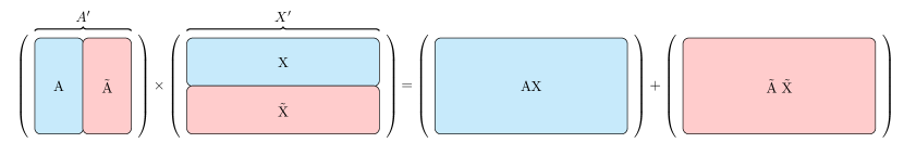
Figure 1. Rectangular A with $n>m$

We summarize our reasoning in the following algorithm.

Algorithm 3 Rectangular Algorithm

1:Generate a $(n-m)\times p$ matrix $Z$ with iid random variables that agree with the model for $X$.

2:Generate a $n\times(n-m)$ matrix $B$ with iid entries (either Gaussian or Rademacher).

3:Run ER-SpUD on $Y^{\prime}=Y+BZ$

4:Remove the rows of $A^{\prime}$ and the columns of $X^{\prime}$ from the output of ER-SpUD.

6. Optimal bound for very sparse random matrices

In this section, we discuss Theorem 1.6. We present a simple algorithm (see below) and use this algorithm to prove Theorem 1.6, obtaining the optimal bound $p=Cn\log n$.

Algorithm 4 Very-sparse Algorithm

1:Partition the columns of Y into a minimum number of groups $G_{i}$ whose members are multiples of each other.

2:Choose representatives of those $G_{i}$ with more than two members to be the columns of A up to scaling.

Proof of Theorem 1.6. Since $A$ is nonsingular, any two columns of $Y$ that are multiples of each other must be linear combinations of the same columns of $A$. For a group $G_{i}$ to have more than two members would require that there be more than two columns in $X$ with their non-zero entries in the same rows.

Definition 6.1.

We say that a set of columns are aligned if they each have more than one nonzero entry and their non-zero entries occur in the same positions.

Lemma 6.2.

The probability that $X$ has more than two aligned columns is $o(1)$.

Thus, the algorithm is likely to yield only columns of $A$. We now need to show that all the columns of $A$ will be outputted with high probability.

Definition 6.3.

We say the column $\mathbf{a}$ of $A$ is k-represented if some group $G_{i}$ consists of multiples of $\mathbf{a}$ and $|G_{i}|=k$. In particular, if no multiple of the $j$th column, $\mathbf{a_{j}}$, shows up in the columns of $Y$ then $\mathbf{a_{j}}$ is $0$-represented. A column is well represented if it is $k$-represented for $k>2$.

Notice that the algorithm will output a multiple of every column that is well represented.

The following lemma finishes the proof of Theorem 1.6.

Lemma 6.4.

The probability that every column $\mathbf{a_{i}}$ is well represented is $1-o(1)$.

6.1. Proofs of Sparse Algorithm

Proof of Lemma 6.2. Given the choice of $\theta$, we know that the number of nonzero entries in any column of $X$ will converge to the Poisson distribution. We ignore the $o(1/n)$ error terms from this approximation in later calculations to alleviate clutter. To calculate the probability, we condition on the number of nonzero entries, and then we bound the probability that three specific columns have the required property, and finally we use the union bound. This yields an upper bound of

$${n\choose 3}\sum_{k\geq 2}\frac{e^{-3c}}{(k!)^{3}}\frac{1}{{n\choose k}^{2}}=o(1)$$

$\square$

Proof of Lemma 6.4. By the union bound,

$${\mathbf{P}}(\exists i\text{ such that }\mathbf{a_{i}}\text{ is not well represented})\leq n{\mathbf{P}}(\mathbf{a_{1}}\text{ is not well represented})$$

Partitioning into disjoint events yields

$${\mathbf{P}}(\mathbf{a_{1}}\text{ is not well represented})=\sum_{j=0}^{2}{\mathbf{P}}(\mathbf{a_{1}}\text{ is }\text{$j$-represented})$$

Notice that a multiple of $\mathbf{a_{1}}$, say $a*\mathbf{a_{1}}$, appears as a column of $Y$ if and only if $a*\mathbf{e_{1}}=(a,0,0,\dots,0)^{T}$, with $a\neq 0$, is $X^{j}$, the $j$th column of $X$, for some $j$. Now, using the Poisson approximation we can bound each term in the summand. For example, for the probability of being $0$-represented, we can divide into the case that $X^{i}$ does not have exactly one non-zero element and the case that $X^{i}$ has exactly one non-zero term but not in the first row. We use $C$ to indicate an absolute constant which may change with each appearance.

$${\mathbf{P}}(\mathbf{a_{1}}\text{ is }\text{$0$-represented})\leq\left((1-ce^{-c})+e^{-c}\frac{n-1}{n}\right)^{p}\leq C\exp(-Cp/n)$$

Similarly,

$${\mathbf{P}}(\mathbf{a_{1}}\text{ is }\text{$1$-represented})\leq n\left(\frac{ce^{-c}}{n}\right)\left((1-ce^{-c})+e^{-c}\frac{n-1}{n}\right)^{p-1}\leq C\exp(-Cp/n)$$

and

$${\mathbf{P}}(\mathbf{a_{1}}\text{ is }\text{$2$-represented})\leq{n\choose 2}\left(\frac{ce^{-c}}{n}\right)^{2}\left((1-ce^{-c})+e^{-c}\frac{n-1}{n}\right)^{p-2}\leq C\exp(-Cp/n)$$

Thus,

$${\mathbf{P}}(\mathbf{a_{1}}\text{ is not well represented})\leq C\exp(\log n-Cp/n)=o(1)$$

for $p=C^{\prime}n\log n$ for a large enough $C^{\prime}$. $\square$

7. Proof of Theorem 1.7

7.1. Lemmas Independent of Symmetry

We first state the necessary lemmas from [15] whose proofs do not use the symmetry of the random variables.

Lemma 7.1.

If $rank(X)=n$, $A$ is nonsingular, and $Y$ can be decomposed into $Y=A^{\prime}X^{\prime}$, then the row spaces of $X^{\prime}$, $X$, and $Y$ are the same.

The general idea is to show that the sparsest vectors in the row-span of $Y$ are the rows of $X$. Since all of the rows of $X^{\prime}$ lie in the row-span of $Y$, intuitively, they can be sparse only when they are multiples of the rows of $X$. Naively, this is because rows of $X$ are likely to have nearly disjoint supports. Thus, any linear combination of them will probably increase the number of nonzero entries.

Lemma 7.2.

Let $\Omega$ be an $n\times p$ Bernoulli($\theta$) matrix with $1/n<\theta<1/4$. For each set $S\subseteq[n]$, let $T_{S}\subseteq[p]$ be the indices of the columns of $\Omega$ that have at least one non-zero entry in some row indexed by $S$.

1. For every set $S$ of size 2,

   $${\mathbf{P}}(|T_{S}|\leq(4/3)\theta p)\leq\exp\left(-\frac{\theta p}{108}\right)$$

2. For every set $S$ of size $\sigma$ with $3\leq\sigma\leq 1/\theta$,

   $${\mathbf{P}}(|T_{S}|\leq(3\sigma/8)\theta p)\leq\exp\left(-\frac{\sigma\theta p}{64}\right)$$

3. For every set $S$ of size $\sigma$ with $1/\theta\leq\sigma$,

   $${\mathbf{P}}(|T_{S}|\leq(1-1/e)p/2)\leq\exp\left(-\frac{(1-1/e)p}{8}\right)$$

7.2. Generalized Lemmas

We will use a result of [14].

Lemma 7.3.

Let $\xi_{1},\dots,\xi_{n}$ be independent centered random variables with variances at least $1$ and fourth moments bounded by $B$. Then there exists $\nu\in(0,1)$ depending only on $B$, such that for every coefficient vector $a=(a_{1},\dots,a_{n})\in S^{n-1}$ the random sum $S=\sum_{k=1}^{n}a_{k}\xi_{k}$ satisfies

$${\mathbf{P}}(|S|<\frac{1}{2})\leq\nu$$

Definition 7.4.

We call a vector $\alpha\in\mathbb{R}^{n}$ fully dense if for all $i\in[n]$, $\alpha_{i}\neq 0$.

Lemma 7.5.

For $b>s$, let $H\in\mathbb{R}^{s\times b}$ be a matrix with one nonzero in each column. Let $R$ be a s-by-b matrix with independent centered random variables with variances at least $1$ and bounded fourth moments. Define $U=H\odot R$ Then the probability that the left nullspace of $U$ contains a fully dense vector is at most

Proof of Lemma 7.5. Let $U=[u_{1}|\dots|u_{b}]$ denote the columns of $U$ and for each $j\in[b]$, let $N_{j}$ be the left nullspace of $[u_{1}|\dots|u_{j}]$. We show that with high probability $N_{b}$ cannot contain a fully dense vector. This can be done by showing that if $N_{j-1}$ contains a fully dense vector then with probability 1/2 the dimension of $N_{j}$ is less than the dimension of $N_{j-1}$. Formally, consider a fully dense vector $\alpha\in N_{j-1}$. If $u_{j}$ contains only one nonzero entry, then $\alpha^{T}u_{j}\neq 0$ reducing the dimension of $N_{j}$. If $u_{j}$ contains more than one non-zero entry, then Lemma 7.3 implies that the probability, over the choice of entries of $R_{j}$, that $\alpha^{T}u_{j}=0$ is less than $1/2$.

Note that the dimension cannot decrease more than $s$ times. For $N_{b}$ to contain a fully dense vector, there must be at least $b-s$ columns for which the dimension of the nullspace does nto decrease. Let $F\subset[b]$ have size $b-s$. The probability that for every $j\in F$, $N_{j-1}$ contains a fully dense vector and that the dimension of $N_{j}$ equals the dimension of $N_{j-1}$ is at most $2^{-b+s-1}$. By the union bound, the probability that $N_{b}$ contains a fully dense vector is at most

$${b\choose{b-s}}2^{-b+s}\leq\left(\frac{eb}{s}\right)^{s}2^{-b+s}\leq 2^{-b+s\log(e^{2}b/s)}$$

$\square$

The proofs of the following lemmas are identical to those in [15] except that they now use our more general Lemma 7.5 along with the lemmas in the previous section.

Lemma 7.6.

For $t>200s$, let $\Omega\in\{0,1\}^{s\times t}$ be any binary matrix with at least one nonzero in each column. Let $R\in\mathbb{R}^{s\times t}$ be a random matrix whose entries are iid random variables, with ${\mathbf{P}}(R_{ij}=0)=0$, and let $U=\Omega\odot R$. Then, the probability that there exists a fully-dense vector $\alpha$ for which $\|\alpha^{T}U\|_{0}\leq t/5$ is at most $2^{-t/25}$.

Lemma 7.7.

If $X=\Omega\odot R$ follows the Bernoulli-Subgaussian model with ${\mathbf{P}}(R_{ij}=0)=0$, $1/n<\theta<1/C$ and $p>Cn\log n$, then the probability that there is a vector $\alpha$ with support of size larger than $1$ for which

$$\|\alpha^{T}X\|_{0}\leq(11/9)\theta p$$

is at most $\exp(-c\theta p)$, and $C,c$ are numerical constants.

7.3. Proof of Theorem 1.7

Say $Y$ can be decomposed as $A^{\prime}X^{\prime}$. From Lemma 7.7, we know that with probability at most $\exp(-c\theta p)$, any linear combination of two or more rows of $X$ has at least $(11/9)\theta p$ nonzeros. By a simple Chernoff bound, the probability that any row of $X$ has more than $(10/9)\theta p$ nonzero entries is bounded by $n\exp(-\theta p/243)$. Thus, the rows of $X$ are likely the sparsest in $row(X)$.

On the previous event of probability at least $1-\exp(-c\theta p)$, $X$ does not have any left null vectors with more than one nonzero entry. Therefore, if the rows of $X$ are nonzero, $X$ will have no nonzero vectors in its left nullspace. The probability that all of the rows of $X$ are nonzero is at least $1-n(1-\theta)^{p}\geq 1-n\exp(-cp)$. From this, by Lemma 7.1, we get $row(X)=row(Y)=row(X^{\prime})$. Hence, we can conclude that every row in $X^{\prime}$ is a scalar multiple of a row of $X$. $\square$

8. Numerical Simulations

We demonstrate that the efficiency of the ER-SpUD algorithm is not improved with larger $p$ values beyond the threshold conjectured. In Figure 2, we have chosen $A$ to be an $n\times n$ matrix of independent $N(0,1)$ random variables. The $n\times p$ matrix $X$ has $k$ randomly chosen non-zero entries which are Rademacher. The graph on the left of Figure 2 is generated with $p=5n\log n$ and the one on the right with $p=5n^{2}\log^{2}n$. For both graphs, $n$ varies from $10$ to $60$ and $k$ from $1$ to $10$. Accuracy is measured in terms of relative error:

$$re(A^{\prime},A)=min_{\Pi,\Lambda}\|A^{\prime}\Lambda\Pi-A\|_{F}/\|A\|_{F}$$

The average relative error over ten trials is reported.

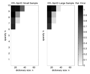
Figure 2. Mean relative errors of ER-SpUD with $p=5n\log n$ versus $p=5n^{2}\log^{2}n$

We then ran our Algorithm 4 in a sparse regime to compare its performance with that of ER-SpUD (see Figure 3. $A$ was as before, but since our algorithm relies on the appearance of 1-sparse columns in $X$, we cannot fix sparsity as in our first experiments. Rather, we vary the Bernoulli parameter $\theta$ from $0.02$ to $0.18$, and the $\chi_{ij}$ are Rademacher. One can see the expected phase transition at which point the matrix $X$ is no longer sparse enough for our algorithm. In the regime for which the algorithm was designed, the relative error of our output is on the same order as that of ER-SpUD. Furthermore, our algorithm runs much quicker and has no trouble with inputs of size up to $n=500$. (The numerical experiments were completed on a Macbook Pro.)

Finally, we compare the outcome of our optimal $p$ value with that of a much larger sample size ($p=O(n^{2}\log^{2}n)$). We let $n$ range from $10$ to $200$ and $\theta$ from $0.01$ to $0.08$. Figure 4 shows that the efficacy of the algorithm is not much improved despite the dramatic increase in $p$. The threshold for failure is identical.

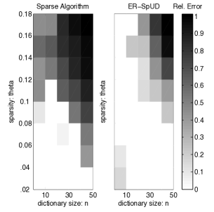
Figure 3. Mean relative errors with varying sparsity $\theta$. Here, $p=5n\log n$.

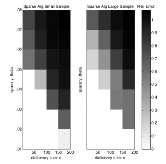
Figure 4. Mean relative errors of Algorithm 4 with $p=5n\log n$ versus $p=5n^{2}\log^{2}n$

References

- [1] Michal Aharon, Michael Elad, and Alfred Bruckstein. The k-svd: An algorithm for designing overcomplete dictionaries for sparse representation. Signal Processing, IEEE Transactions on, 54(11):4311–4322, 2006.
- [2] Michal Aharon, Michael Elad, and Alfred M Bruckstein. On the uniqueness of overcomplete dictionaries, and a practical way to retrieve them. Linear algebra and its applications, 416(1):48–67, 2006.
- [3] Jean Bourgain, Van H Vu, and Philip Matchett Wood. On the singularity probability of discrete random matrices. Journal of Functional Analysis, 258(2):559–603, 2010.
- [4] Kjersti Engan, Sven Ole Aase, and J Hakon Husoy. Method of optimal directions for frame design. In Acoustics, Speech, and Signal Processing, 1999. Proceedings., 1999 IEEE International Conference on, volume 5, pages 2443–2446. IEEE, 1999.
- [5] X Fernique. Regularite de processus gaussien. In Invent Math., pages 304–321. 1971.
- [6] Pando Georgiev, Fabian Theis, and Andrzej Cichocki. Blind source separation and sparse component analysis of overcomplete mixtures. In Acoustics, Speech, and Signal Processing, 2004. Proceedings.(ICASSP’04). IEEE International Conference on, volume 5, pages V–493. IEEE, 2004.
- [7] Lee-Ad Gottlieb and Tyler Neylon. Matrix sparsification and the sparse null space problem. In Approximation, Randomization, and Combinatorial Optimization. Algorithms and Techniques, pages 205–218. Springer, 2010.
- [8] Florent Jaillet, Rémi Gribonval, Mark D Plumbley, and Hadi Zayyani. An l1 criterion for dictionary learning by subspace identification. In Acoustics Speech and Signal Processing (ICASSP), 2010 IEEE International Conference on, pages 5482–5485. IEEE, 2010.
- [9] Kenneth Kreutz-Delgado, Joseph F Murray, Bhaskar D Rao, Kjersti Engan, Te-Won Lee, and Terrence J Sejnowski. Dictionary learning algorithms for sparse representation. Neural computation, 15(2):349–396, 2003.
- [10] Liangyue Li, Sheng Li, and Yun Fu. Discriminative dictionary learning with low-rank regularization for face recognition. In Automatic Face and Gesture Recognition (FG), 2013 10th IEEE International Conference and Workshops on, pages 1–6. IEEE, 2013.
- [11] Julien Mairal, Francis Bach, Jean Ponce, and Guillermo Sapiro. Online dictionary learning for sparse coding. In Proceedings of the 26th Annual International Conference on Machine Learning, pages 689–696. ACM, 2009.
- [12] Bruno A Olshausen et al. Emergence of simple-cell receptive field properties by learning a sparse code for natural images. Nature, 381(6583):607–609, 1996.
- [13] Mark D Plumbley. Dictionary learning for l1-exact sparse coding. In Independent Component Analysis and Signal Separation, pages 406–413. Springer, 2007.
- [14] Mark Rudelson and Roman Vershynin. The littlewood–offord problem and invertibility of random matrices. Advances in Mathematics, 218(2):600–633, 2008.
- [15] Daniel A Spielman, Huan Wang, and John Wright. Exact recovery of sparsely-used dictionaries. In Proceedings of the Twenty-Third international joint conference on Artificial Intelligence, pages 3087–3090. AAAI Press, 2013.
- [16] Michel Talagrand. Majorizing measures: the generic chaining. The Annals of Probability, pages 1049–1103, 1996.
- [17] John Wright, Allen Y Yang, Arvind Ganesh, Shankar S Sastry, and Yi Ma. Robust face recognition via sparse representation. Pattern Analysis and Machine Intelligence, IEEE Transactions on, 31(2):210–227, 2009.
- [18] Qiang Zhang and Baoxin Li. Discriminative k-svd for dictionary learning in face recognition. In Computer Vision and Pattern Recognition (CVPR), 2010 IEEE Conference on, pages 2691–2698. IEEE, 2010.
- [19] Michael Zibulevsky. Blind source separation with relative newton method. In Proc. ICA, volume 2003, pages 897–902, 2003.
- [20] Michael Zibulevsky and Barak A Pearlmutter. Blind source separation by sparse decomposition. In AeroSense 2000, pages 165–174. International Society for Optics and Photonics, 2000.