Decentralized Learning for Wireless Communications and Networking

Abstract

This chapter deals with decentralized learning algorithms for in-network processing of graph-valued data. A generic learning problem is formulated and recast into a separable form, which is iteratively minimized using the alternating-direction method of multipliers (ADMM) so as to gain the desired degree of parallelization. Without exchanging elements from the distributed training sets and keeping inter-node communications at affordable levels, the local (per-node) learners consent to the desired quantity inferred globally, meaning the one obtained if the entire training data set were centrally available. Impact of the decentralized learning framework to contemporary wireless communications and networking tasks is illustrated through case studies including target tracking using wireless sensor networks, unveiling Internet traffic anomalies, power system state estimation, as well as spectrum cartography for wireless cognitive radio networks.

1 Introduction

This chapter puts forth an optimization framework for learning over networks, that entails decentralized processing of training data acquired by interconnected nodes. Such an approach is of paramount importance when communication of training data to a central processing unit is prohibited due to e.g., communication cost or privacy reasons. The so-termed in-network processing paradigm for decentralized learning is based on successive refinements of local model parameter estimates maintained at individual network nodes. In a nutshell, each iteration of this broad class of fully decentralized algorithms comprises: (i) a communication step where nodes exchange information with their neighbors through e.g., the shared wireless medium or Internet backbone; and (ii) an update step where each node uses this information to refine its local estimate. Devoid of hierarchy and with their decentralized in-network processing, local e.g., estimators should eventually consent to the global estimator sought, while fully exploiting existing spatiotemporal correlations to maximize estimation performance. In most cases, consensus can formally be attained asymptotically in time. However, a finite number of iterations will suffice to obtain results that are sufficiently accurate for all practical purposes.

In this context, the approach followed here entails reformulating a generic learning task as a convex constrained optimization problem, whose structure lends itself naturally to decentralized implementation over a network graph. It is then possible to capitalize upon this favorable structure by resorting to the alternating-direction method of multipliers (ADMM), an iterative optimization method that can be traced back to Glowinski_Marrocco_ADMM_1975 (see also Gabay_Mercier_ADMM_1976 ), and which is specially well-suited for parallel processing bertsi97book ; Boyd_ADMM . This way simple decentralized recursions become available to update each node’s local estimate, as well as a vector of dual prices through which network-wide agreement is effected.

Problem statement. Consider a network of $n$ nodes in which scarcity of power and bandwidth resources encourages only single-hop inter-node communications, such that the $i$-th node communicates solely with nodes $j$ in its single-hop neighborhood ${\cal N}_{i}$. Inter-node links are assumed symmetric, and the network is modeled as an undirected graph whose vertices are the nodes and its edges represent the available communication links. As it will become clear through the different application domains studied here, nodes could be wireless sensors, wireless access points (APs), electrical buses, sensing cognitive radios, or routers, to name a few examples. Node $i$ acquires $m_{i}$ measurements stacked in the vector $\mathbf{y}_{i}\in\mathbb{R}^{m_{i}}$ containing information about the unknown model parameters in $\mathbf{s}\in\mathbb{R}^{p}$, which the nodes need to estimate. Let $\mathbf{y}:=[\mathbf{y}_{1}^{\top},\ldots,\mathbf{y}_{n}^{\top}]^{\top}\in\mathbb{R}^{\sum_{i}m_{i}}$ collect measurements acquired across the entire network. Many popular centralized schemes obtain an estimate $\hat{\mathbf{s}}$ as follows

$$\hat{\mathbf{s}}\in\arg\min_{\mathbf{s}}\textstyle\sum_{i=1}^{n}f_{i}(\mathbf{s};\mathbf{y}_{i}).$$ (1)

In the decentralized learning problem studied here though, the summands $f_{i}$ are assumed to be local cost functions only known to each node $i$. Otherwise sharing this information with a centralized processor, also referred to as fusion center (FC), can be challenging in various applications of interest, or, it may be even impossible in e.g., wireless sensor networks (WSNs) operating under stringent power budget constraints. In other cases such as the Internet or collaborative healthcare studies, agents may not be willing to share their private training data ${\bf y}_{i}$ but only the learning results. Performing the optimization (1) in a centralized fashion raises robustness concerns as well, since the central processor represents an isolated point of failure.

In this context, the objective of this chapter is to develop a decentralized algorithmic framework for learning tasks, based on in-network processing of the locally available data. The described setup naturally suggests three characteristics that the algorithms should exhibit: c1) each node $i=1,\ldots,n$ should obtain an estimate of ${\bf s}$, which coincides with the corresponding solution $\hat{{\bf s}}$ of the centralized estimator (1) that uses the entire data $\{{\bf y}_{i}\}_{i=1}^{n}$; c2) processing per node should be kept as simple as possible; and c3) the overhead for inter-node communications should be affordable and confined to single-hop neighborhoods. It will be argued that such an ADMM-based algorithmic framework can be useful for contemporary applications in the domain of wireless communications and networking.

Prior art. Existing decentralized solvers of (1) can be classified in two categories: C1) those obtained by modifying centralized algorithms and operating in the primal domain; and C2) those handling an equivalent constrained form of (1) (see (2) in Section 2), and operating in the primal-dual domain.

Primal-domain algorithms under C1 include the (sub)gradient method and its variants Nedic2009 ; Ram2010 ; Yuan2013 ; Jakovetic2013 , the incremental gradient method Rabbat2005-inc , the proximal gradient method Chen2012 , and the dual averaging method Duchi2012 ; Tsianos2012-acc . Each node in these methods, averages its local iterate with those of neighbors and descends along its local negative (sub)gradient direction. However, the resultant algorithms are limited to inexact convergence when using constant stepsizes Nedic2009 ; Yuan2013 . If diminishing stepsizes are employed instead, the algorithms can achieve exact convergence at the price of slowing down speed Jakovetic2013 ; Rabbat2005-inc ; Duchi2012 . A constant-stepsize exact first-order algorithm is also available to achieve fast and exact convergence, by correcting error terms in the distributed gradient iteration with two-step historic information Shi2014-extra .

Primal-dual domain algorithms under C2 solve an equivalent constrained form of (1), and thus drive local solutions to reach global optimality. The dual decomposition method is hence applicable because (sub)gradients of the dual function depend on local and neighboring iterates only, and can thus be computed without global cooperation Rabbat2005 . ADMM modifies the dual decomposition by regularizing the constraints with a quadratic term, which improves numerical stability as well as rate of convergence, as will be demonstrated later in this chapter. Per ADMM iteration, each node solves a subproblem that can be demanding. Fortunately, these subproblems can be solved inexactly by running one-step gradient or proximal gradient descent iterations, which markedly mitigate the computation burden Ling2014-icassp ; Chang2014-icassp . A sequential distributed ADMM algorithm can be found in Wei2012 .

Chapter outline. The remainder of this chapter is organized as follows. Section 2 describes a generic ADMM framework for decentralized learning over networks, which is at the heart of all algorithms described in the chapter and was pioneered in sg06asilomar ; srg08tsp for in-network estimation using WSNs. Section 3 focuses on batch estimation as well as (un)supervised inference, while Section 4 deals with decentralized adaptive estimation and tracking schemes where network nodes collect data sequentially in time. Internet traffic anomaly detection and spectrum cartography for wireless CR networks serve as motivating applications for the sparsity-regularized rank minimization algorithms developed in Section 5. Fundamental results on the convergence and convergence rate of decentralized ADMM are stated in Section 6.

2 In-Network Learning with ADMM in a Nutshell

Since local summands in (1) are coupled through a global variable $\mathbf{s}$, it is not straightforward to decompose the unconstrained optimization problem in (1). To overcome this hurdle, the key idea is to introduce local variables ${\cal S}:=\{\mathbf{s}_{i}\}_{i=1}^{n}$ which represent local estimates of $\mathbf{s}$ per network node $i$ sg06asilomar ; srg08tsp . Accordingly, one can formulate the constrained minimization problem

$$\{\hat{\mathbf{s}}_{i}\}_{i=1}^{n}\in\arg\min_{{\cal S}}\textstyle\sum_{i=1}^{n}f_{i}(\mathbf{s}_{i};\mathbf{y}_{i}),\;\;\;\;\textrm{s. to }~{}~{}~{}\mathbf{s}_{i}=\mathbf{s}_{j},\;j\in{\cal N}_{i}.$$ (2)

The “consensus” equality constraints in (2) ensure that local estimates coincide within neighborhoods. Further, if the graph is connected then consensus naturally extends to the whole network, and it turns out that problems (1) and (2) are equivalent in the sense that $\hat{\mathbf{s}}=\hat{\mathbf{s}}_{1}=\ldots=\hat{\mathbf{s}}_{n}$ srg08tsp . Interestingly, the formulation in (2) exhibits a separable structure that is amenable to decentralized minimization. To leverage this favorable structure, the alternating direction method of multipliers (ADMM), see e.g., (bertsi97book, , pg. 253-261), can be employed here to minimize (2) in a decentralized fashion. This procedure will yield a distributed estimation algorithm whereby local iterates $\mathbf{s}_{i}(k)$, with $k$ denoting iterations, provably converge to the centralized estimate $\hat{\mathbf{s}}$ in (1); see also Section 6.

To facilitate application of ADMM, consider the auxiliary variables ${\cal Z}:=\{\mathbf{z}_{i}^{j}\}_{j\in{\cal N}_{i}}$, and reparameterize the constraints in (2) with the equivalent ones

$$\{\hat{\mathbf{s}}_{i}\}_{i=1}^{n} {}\in\arg\min_{{\cal S}}\textstyle\sum_{i=1}^{n}f_{i}(\mathbf{s}_{i};\mathbf{y}_{i}),$$

s. to $$~{}~{}~{}\mathbf{s}_{i}=\mathbf{z}_{i}^{j}\textrm{ and }\mathbf{s}_{j}=\mathbf{z}_{i}^{j},\;\;i=1,\ldots,n,\;\;j\in{\cal N}_{i},\;\;i\neq j.$$ (3)

Variables $\mathbf{z}_{i}^{j}$ are only used to derive the local recursions but will be eventually eliminated. Attaching Lagrange multipliers ${\cal V}:=\{\{\bar{\mathbf{v}}_{i}^{j}\}_{j\in{\cal N}_{i}},\{\tilde{\mathbf{v}}_{i}^{j}\}_{j\in{\cal N}_{i}}\}_{i=1}^{n}$ to the constraints (2), consider the augmented Lagrangian function

$$L_{c}[{\cal S},{\cal Z},{\cal V}]=\sum_{i=1}^{n}f_{i}(\mathbf{s}_{i};\mathbf{y}_{i}) +\sum_{i=1}^{n}\sum_{j\in{\cal N}_{i}}\left[(\bar{\mathbf{v}}_{i}^{j})^{\top}(\mathbf{s}_{i}-\mathbf{z}_{i}^{j})+(\tilde{{\bf v}}_{i}^{j})^{\top}(\mathbf{s}_{j}-\mathbf{z}_{i}^{j})\right]$$

$$+\frac{c}{2}\sum_{i=1}^{n}\sum_{j\in{\cal N}_{i}}\left[\|\mathbf{s}_{i}-\mathbf{z}_{i}^{j}\|^{2}+\|\mathbf{s}_{j}-\mathbf{z}_{i}^{j}\|^{2}\right]$$ (4)

where the constant $c>0$ is a penalty coefficient. To minimize (2), ADMM entails an iterative procedure comprising three steps per iteration $k=1,2,\ldots$

[S1]

Multiplier updates:

$$\bar{{\mathbf{v}}}_{i}^{j}(k) =\bar{{\mathbf{v}}}_{i}^{j}(k-1)+c[{\mathbf{s}}_{i}(k)-{\mathbf{z}}_{i}^{j}(k)]$$

$$\tilde{{\mathbf{v}}}_{i}^{j}(k) =\tilde{{\mathbf{v}}}_{i}^{j}(k-1)+c[{\mathbf{s}}_{j}(k)-{\mathbf{z}}_{i}^{j}(k)].$$

[S2]

Local estimate updates:

$${\cal S}(k+1)=\mbox{arg}\>\min_{{\cal S}}L_{c}\left[{\cal S},{\cal Z}(k),{\cal V}(k)\right].$$

[S3]

Auxiliary variable updates:

$${\cal Z}(k+1)=\mbox{arg}\>\min_{{\cal Z}}L_{c}\left[{\cal S}(k+1),{\cal Z},{\cal V}(k)\right]$$

where $i=1,\ldots,n$ and $j\in{\cal N}_{i}$ in [S1]. Reformulating the generic learning problem (1) as (2) renders the augmented Lagrangian in (2) highly decomposable. The separability comes in two flavors, both with respect to the sets ${\cal S}$ and ${\cal Z}$ of primal variables, as well as across nodes $i=1,\ldots,n$. This in turn leads to highly parallelized, simplified recursions corresponding to the aforementioned steps [S1]-[S3]. Specifically, as detailed in e.g., srg08tsp ; sgrr08tsp ; SMG_D_LMS ; pfacgg10jmlr ; mateos_dlasso ; mmg13tsp , it follows that if the multipliers are initialized to zero, the ADMM-based decentralized algorithm reduces to the following updates carried out locally at every node In-network learning algorithm at node $i$, for $k=1,2,\ldots$:

$${\bf v}_{i}(k) ={\bf v}_{i}(k-1)+c\sum_{j\in{\cal N}_{i}}[{\bf s}_{i}(k)-{\bf s}_{j}(k)]$$ (5)

$${\bf s}_{i}(k+1) =\arg\min_{{\bf s}_{i}}\left\{f_{i}(\mathbf{s}_{i};\mathbf{y}_{i})+{\bf v}_{i}^{\top}(k){\bf s}_{i}+c\sum_{j\in{\cal N}_{i}}\left\|{\bf s}_{i}-\frac{{\bf s}_{i}(k)+{\bf s}_{j}(k)}{2}\right\|^{2}\right\}$$ (6)

where ${\bf v}_{i}(k):=2\sum_{j\in{\cal N}_{i}}\bar{{\bf v}}_{i}^{j}(k)$, and all initial values are set to zero.

Recursions (5) and (6) entail local updates, which comprise the general purpose ADMM-based decentralized learning algorithm. The inherently redundant set of auxiliary variables in ${\cal Z}$ and corresponding multipliers have been eliminated. Each node, say the $i$-th one, does not need to separately keep track of all its non-redundant multipliers $\{\bar{{\mathbf{v}}}_{i}^{j}(k)\}_{j\in{\cal N}_{i}}$, but only to update the (scaled) sum ${\mathbf{v}}_{i}(k)$. In the end, node $i$ has to store and update only two $p$-dimensional vectors, namely $\{{\bf s}_{i}(k)\}$ and $\{{\bf v}_{i}(k)\}$. A unique feature of in-network processing is that nodes communicate their updated local estimates $\{{\bf s}_{i}\}$ (and not their raw data ${\bf y}_{i}$) with their neighbors, in order to carry out the tasks (5)-(6) for the next iteration.

As elaborated in Section 6, under mild assumptions on the local costs one can establish that $\lim_{k\to\infty}{\bf s}_{i}(k)=\hat{{\bf s}}$, for $i=1,\ldots,n$. As a result, the algorithm asymptotically attains consensus and the performance of the centralized estimator [cf. (1)].

3 Batch In-Network Estimation and Inference

3.1 Decentralized Signal Parameter Estimation

Many workhorse estimation schemes such as maximum likelihood estimation (MLE), least-squares estimation (LSE), best linear unbiased estimation (BLUE), as well as linear minimum mean-square error estimation (LMMSE) and the maximum a posteriori (MAP) estimation, all can be formulated as a minimization task similar to (1); see e.g. Estimation_Theory . However, the corresponding centralized estimation algorithms fall short in settings where both the acquired measurements and computational capabilities are distributed among multiple spatially scattered sensing nodes, which is the case with WSNs. Here we outline a novel batch decentralized optimization framework building on the ideas in Section 2, that formulates the desired estimator as the solution of a separable constrained convex minimization problem tackled via ADMM; see e.g., bertsi97book ; Boyd_ADMM ; srg08tsp ; sgrr08tsp for further details on the algorithms outlined here.

Depending on the estimation technique utilized, the local cost functions $f_{i}(\cdot)$ in (1) should be chosen accordingly, see e.g., Estimation_Theory ; srg08tsp ; sgrr08tsp . For instance, when $\mathbf{s}$ is assumed to be an unknown deterministic vector, then:

• If $\hat{\mathbf{s}}$ corresponds to the centralized MLE then $f_{i}(\mathbf{s};\mathbf{y}_{i})=-\ln[p_{i}(\mathbf{y}_{i};\mathbf{s})]$ is the negative log-likelihood capturing the data probability density function (pdf), while the network-wide data $\{\mathbf{y}_{i}\}_{i=1}^{n}$ are assumed statistically independent.

• If $\hat{\mathbf{s}}$ corresponds to the BLUE (or weighted least-squares estimator) then $f_{i}(\mathbf{s};\mathbf{y}_{i})=(1/2)\|\bm{\Sigma}_{y_{i}}^{-1/2}(\mathbf{y}_{i}-\mathbf{H}_{i}\mathbf{s})\|^{2}$, where $\bm{\Sigma}_{y_{i}}$ denotes the covariance of the data $\mathbf{y}_{i}$, and $\mathbf{H}_{i}$ is a known fitting matrix.

When $\mathbf{s}$ is treated as a random vector, then:

• If $\hat{\mathbf{s}}$ corresponds to the centralized MAP estimator then $f_{i}(\mathbf{s};\mathbf{y}_{i})=-(\ln[p_{i}(\mathbf{y}_{i}|\mathbf{s})]+n^{-1}\ln[p(\mathbf{s})])$ accounts for the data pdf, and $p(\mathbf{s})$ for the prior pdf of $\mathbf{s}$, while data $\{\mathbf{y}_{i}\}_{i=1}^{n}$ are assumed conditionally independent given $\mathbf{s}$.

• If $\hat{\mathbf{s}}$ corresponds to the centralized LMMSE then $f_{i}(\mathbf{s};\mathbf{y}_{i})=(1/2)\|\mathbf{s}-n\bm{\Sigma}_{sy_{i}}\mathbf{u}^{i}\|_{2}^{2}$, where $\bm{\Sigma}_{sy_{i}}$ denotes the cross-covariance of $\mathbf{s}$ with $\mathbf{y}_{i}$, while $\mathbf{u}^{i}$ stands for the $i$-th $m_{i}\times 1$ block subvector of $\mathbf{u}=\bm{\Sigma}_{y}^{-1}\mathbf{y}$.

Substituting in (6) the specific $f_{i}(\mathbf{s};\mathbf{y}_{i})$ for each of the aforementioned estimation tasks, yields a family of batch ADMM-based decentralized estimation algorithms. The decentralized BLUE algorithm will be described in this section as an example of decentralized linear estimation.

Recent advances in cyber-physical systems have also stressed the need for decentralized nonlinear least-squares (LS) estimation. Monitoring the power grid for instance, is challenged by the nonconvexity arising from the nonlinear AC power flow model; see e.g., (Wollenberg-book, , Ch. 4), while the interconnection across local transmission systems motivates their operators to collaboratively monitor the global system state. Interestingly, this nonlinear (specifically quadratic) estimation task can be convexified to a semidefinite program (SDP) (Boyd_Convex, , pg. 168), for which a decentralized semidefinite programming (SDP) algorithm can be developed by leveraging the batch ADMM; see also Wen2010 for an ADMM-based centralized SDP precursor.

Decentralized BLUE

The minimization involved in (6) can be performed locally at sensor $i$ by employing numerical optimization techniques Boyd_Convex . There are cases where the minimization in (6) yields a closed-form and easy to implement updating formula for $\mathbf{s}_{i}(k+1)$. If for example network nodes wish to find the BLUE estimator in a distributed fashion, the local cost is $f_{i}(\mathbf{s};\mathbf{y}_{i})=(1/2)\|\bm{\Sigma}_{y_{i}}^{-1/2}(\mathbf{y}_{i}-\mathbf{H}_{i}\mathbf{s})\|^{2}$, and (6) becomes a strictly convex unconstrained quadratic program which admits the following closed-form solution (see details in srg08tsp ; MSG_D_RLS )

$$\mathbf{s}_{i}(k+1) =\left(\mathbf{H}_{i}^{\top}\bm{\Sigma}_{y_{i}}^{-1}\mathbf{H}_{i}+2c|{\cal N}_{i}|\mathbf{I}_{p}\right)^{-1}\left[\mathbf{H}_{i}^{\top}\bm{\Sigma}_{y_{i}}^{-1}\mathbf{y}_{i}-\mathbf{v}_{i}(k)+c\sum_{j\in{\cal N}_{i}}\left(\mathbf{s}_{i}(k)+\mathbf{s}_{j}(k)\right)\right].$$ (7)

The pair (5) and (7) comprise the decentralized (D-) BLUE algorithm sg06asilomar ; srg08tsp . For the special case where each node acquires unit-variance scalar observations $y_{i}$, there is no fitting matrix and $s$ is scalar (i.e., $p=1$); D-BLUE offers a decentralized algorithm to obtain the network-wide sample average $\hat{s}=(1/n)\sum_{i=1}^{n}y_{i}$. The update rule for the local estimate is obtained by suitably specializing (7) to

$$s_{i}(k+1) =\left(1+2c|{\cal N}_{i}|\right)^{-1}\left[y_{i}-v_{i}(k)+c\sum_{j\in{\cal N}_{i}}\left(s_{i}(k)+s_{j}(k)\right)\right].$$ (8)

Different from existing distributed averaging approaches Barbarossa_Scu_Coupled_Osci ; dimakis10 ; Consensus_Averaging ; xbk07jpdc , the ADMM-based one originally proposed in sg06asilomar ; srg08tsp allows the decentralized computation of general nonlinear estimators that may be not available in closed form and cannot be expressed as “averages.” Further, the obtained recursions exhibit robustness in the presence of additive noise in the inter-node communication links.

Decentralized SDP

Consider now that each scalar $y_{i}^{\ell}$ in ${\bf y}_{i}$ adheres to a quadratic measurement model in ${\mathbf{s}}$ plus additive Gaussian noise, where the centralized MLE requires solving a nonlinear least-squares problem. To tackle the nonconvexity due to the quadratic dependence, the task of estimating the state ${\bf s}$ can be reformulated as that of estimating the outer-product matrix ${\mathbf{S}}:={\bf s}{\bf s}^{\top}$. In this reformulation $y_{i}^{\ell}$ is a linear function of ${\bf S}$, given by $\textsf{Tr}({\bf H}_{i}^{\ell}{\bf S})$ with a known matrix ${\bf H}_{i}^{\ell}$ hzgg_jstsp14 . Motivated by the separable structure in (2), the nonlinear estimation problem can be similarly formulated as

$$\{\hat{\mathbf{S}}_{i}\}_{i=1}^{n} {}\in\arg\min\sum_{i=1}^{n}\sum_{\ell}\left[y_{i}^{\ell}-\textsf{Tr}({\bf H}_{i}^{\ell}{\bf S})\right]^{2},$$

s. to $$~{}~{}~{}\mathbf{S}_{i}=\mathbf{Z}_{i}^{j}\textrm{ and }\mathbf{S}_{j}=\mathbf{Z}_{i}^{j},\;\;i=1,\ldots,n,\;\;j\in{\cal N}_{i},\;\;i\neq j$$

$$~{}~{}~{}{\bf S}_{i}\succeq\mathbf{0}\textrm{ and }\textsf{rank}({\bf S}_{i})=1,\;\;i=1,\ldots,n~{}$$ (9)

where the positive-semidefiniteness and rank constraints ensure that each matrix ${\bf S}_{i}$ is an outer-product matrix. By dropping the non-convex rank constraints, the problem (3.1) becomes a convex semidefinite program (SDP), which can be solved in a decentralized fashion by adopting the batch ADMM iterations (5) and (6).

This decentralized SDP approach has been successfully employed for monitoring large-scale power networks gg_spmag13 . To estimate the complex voltage phasor all nodes (a.k.a. power system state), measurements are collected on real/reactive power and voltage magnitude, all of which have quadratic dependence on the unknown states. Gauss-Newton iterations have been the ‘workhorse’ tool for this nonlinear estimation problem; see e.g., SE_book ; Wollenberg-book . However, the iterative linearization therein could suffer from convergence issues and local optimality, especially due to the increasing variability in power grids with high penetration of renewables. With improved communication capabilities, decentralized state estimation among multiple control centers has attracted growing interest; see Fig. 1 illustrating three interconnected areas aiming to achieve the centralized estimation collaboratively.

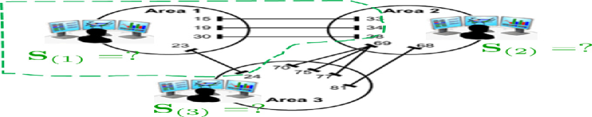
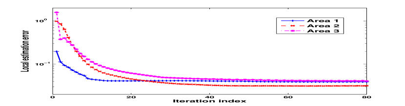
Figure 1: (Left:) Schematic of collaborative power system state estimation among control centers of three interconnected networks (IEEE 118-bus test case). (Right:) Local state estimation error vs. iteration number using the decentralized SDP-based state estimation method.

A decentralized SDP-based state estimator has been developed in hzgg_jstsp14 with reduced complexity compared to (3.1). The resultant algorithm involves only internal voltages and those of next-hop neighbors in the local matrix ${\bf S}_{(i)}$; e.g., in Fig. 1 ${\bf S}_{(1)}$ is identified by the dashed lines. Interestingly, the positive-semidefiniteness constraint for the overall ${\bf S}$ decouples nicely into that of all local $\{{\bf S}_{i}\}$, and the estimation error converges to the centralized performance within only a dozen iterations. The decentralized SDP framework has successfully addressed a variety of power system operational challenges, including a distributed microgrid optimal power flow solver in edhzgg_tsg13 ; see also gg_spmag13 for a tutorial overview of these applications.

3.2 Decentralized Inference

Along with decentralized signal parameter estimation, a variety of inference tasks become possible by relying on the collaborative sensing and computations performed by networked nodes. In the special context of resource-constrained WSNs deployed to determine the common messages broadcast by a wireless AP, the relatively limited node reception capability makes it desirable to design a decentralized detection scheme for all sensors to attain sufficient statistics for the global problem. Another exciting application of WSNs is environmental monitoring for e.g., inferring the presence or absence of a pollutant over a geographical area. Limited by the local sensing capability, it is important to develop a decentralized learning framework such that all sensors can collaboratively approach the performance as if the network wide data had been available everywhere (or at a FC for that matter). Given the diverse inference tasks, the challenge becomes how to design the best inter-node information exchange schemes that would allow for minimal communication and computation overhead in specific applications.

Decentralized Detection

Message decoding. A decentralized detection framework is introduced here for the message decoding task, which is relevant for diverse wireless communications and networking scenarios. Consider an AP broadcasting a $p\times 1$ coded block ${\bf s}$ to a network of sensors, all of which know the codebook ${\mathcal{C}}$ that ${\bf s}$ belongs to. For simplicity assume binary codewords, and that each node $i=1,\ldots,n$ receives a same-length block of symbols ${\bf y}_{i}$ through a discrete, memoryless, symmetric channel that is conditionally independent across sensors. Sensor $i$ knows its local channel from the AP, as characterized by the conditional pdf $p(y_{il}|s_{l})$ per bit $l$. Due to conceivably low signal-to-noise-ratio (SNR) conditions, each low-cost sensor may be unable to reliably decode the message. Accordingly, the need arises for information exchanges among single-hop neighboring sensors to achieve the global (that is, centralized) error performance. Given ${\bf y}_{i}$ per sensor $i$, the assumption on memoryless and independent channels yields the centralized maximum-likelihood (ML) decoder as

$$\hat{{\bf s}}^{DEC}=\arg\max_{{\bf s}\in{\mathcal{C}}}p(\{{\bf y}_{i}\}_{i=1}^{n}|{\bf s})=\arg\min_{{\bf s}\in{\mathcal{C}}}\textstyle\sum_{l=1}^{p}\sum_{i=1}^{n}\left[-\log p(y_{il}|s_{l})\right].$$ (10)

ML decoding amounts to deciding the most likely codeword among multiple candidate ones and, in this sense, it can be viewed as a test of multiple hypotheses. In this general context, belief propagation approaches have been developed in sas06tsp , so that all nodes can cooperate to learn the centralized likelihood per hypothesis. However, even for linear binary block codes, the number of hypotheses, namely the cardinality of ${\mathcal{C}}$, grows exponentially with the codeword length. This introduces high communication and computation burden for the low-cost sensor designs.

The key here is to extract minimal sufficient statistics for the centralized decoding problem. For binary codes, the log-likelihood terms in (10) become $\log p(y_{il}|s_{l})=-\gamma_{il}s_{l}+\log p(y_{il}|s_{l}=0)$, where

$$\gamma_{il}:=\log\left(\frac{p(y_{il}|s_{l}=0)}{p(y_{il}|s_{l}=1)}\right)$$ (11)

is the local log-likelihood ratio (LLR) for the bit $s_{l}$ at sensor $i$. Ignoring all constant terms $\log p(y_{il}|s_{l}=0)$, the ML decoding objective ends up only depending on the sum LLRs, as given by $\hat{{\bf s}}_{ML}=\arg\min_{{\bf s}\in{\mathcal{C}}}\sum_{l=1}^{p}(\sum_{i=1}^{n}\gamma_{il})s_{l}$. Clearly, the sufficient statistic for solving (10) is the sum of all local LLR terms, or equivalently, the average $\bar{\gamma}_{l}=(1/n)\sum_{i=1}^{n}\gamma_{il}$ for each bit $l$. Interestingly, the average of $\{\gamma_{il}\}_{i=1}^{n}$ is one instance of the BLUE discussed in Section 3.1 when $\bm{\Sigma}_{y,i}={\bf H}_{j}={\bf I}_{p\times p}$, since

$$\bar{\gamma}_{l}=\textstyle\arg\min_{\gamma}\sum_{i=1}^{n}(\gamma_{il}-\gamma)^{2}.$$ (12)

This way, the ADMM-based decentralized learning framework in Section 2 allows for all sensors to collaboratively attain the sufficient statistic for the decoding problem (10) via in-network processing. Each sensor only needs to estimate a vector of the codeword length $p$, which bypasses the exponential complexity under the framework of belief propagation. As shown in hzggac08tsp , decentralized soft decoding is also feasible since the a posteriori probability (APP) evaluator also relies on LLR averages which are sufficient statistics, where extensions to non-binary alphabet codeword constraints and random failing inter-sensor links are also considered.

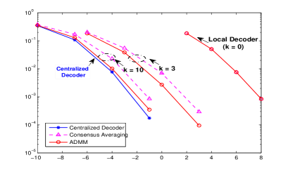
Figure 2: BER vs. SNR (in dB) curves depicting the local ML decoder vs. the consensus-averaging decoder vs. the ADMM-based approach vs. the centralized ML decoder benchmark.

The bit error rate (BER) versus SNR plot in Fig. 2 demonstrates the performance of ADMM-based in-network decoding of a convolutional code with $p=60$ and $|{\mathcal{C}}|=40$. This numerical test involves $n=10$ sensors and AWGN AP-sensor channels with $\sigma_{i}^{2}=10^{-SNR_{i}/10}$. Four schemes are compared: (i) the local ML decoder based on per-sensor data only (corresponds to the curve marked as $k=0$ since it is used to initialize the decentralized iterations); (ii) the centralized benchmark ML decoder (corresponds to $k=\infty$); (iii) the in-network decoder which forms $\bar{\gamma}_{l}$ using “consensus-averaging” linear iterations Consensus_Averaging ; and, (iv) the ADMM-based decentralized algorithm. Indeed, the ADMM-based decoder exhibits faster convergence than its consensus-averaging counterpart; and surprisingly, only 10 iterations suffice to bring the decentralized BER very close to the centralized performance.

Message demodulation. In a related detection scenario the common AP message ${\bf s}$ can be mapped to a space-time matrix, with each entry drawn from a finite alphabet ${\mathcal{A}}$. The received block ${\bf y}_{i}$ per sensor $i$ typically admits a linear input/output relationship ${\bf y}_{i}={\mathbf{H}}_{i}~{}{\bf s}+{\mbox{\boldmath$\epsilon$}}_{i}$. Matrix ${\mathbf{H}}_{i}$ is formed from the fading AP-sensor channel, and ${\mbox{\boldmath$\epsilon$}}_{i}$ stands for the additive white Gaussian noise of unit variance, that is assumed uncorrelated across sensors. Since low-cost sensors have very limited budget on number of antennas compared to the AP, the length of ${\bf y}_{i}$ is much shorter than ${\bf s}$ (i.e., $m_{i}<p$). Hence, the local linear demodulator using $\{{\bf y}_{i},{\mathbf{H}}_{i}\}$ may not even be able to identify ${\bf s}$. Again, it is critical for each sensor $i$ to cooperate with its neighbors to collectively form the global ML demodulator

$${\hat{\mathbf{s}}}^{DEM}=\arg\max_{{\bf s}\in{\mathcal{A}}^{N}}\textstyle-\!\sum_{i=1}^{n}\|{\bf y}_{i}-{\mathbf{H}}_{i}{\bf s}\|^{2}\!\displaystyle=\arg\max_{{\bf s}\in{\mathcal{A}}^{N}}\!\textstyle\left\{\!2\!\Big{(}\sum_{i=1}^{n}{\bf r}_{i}\Big{)}^{\top}\!\!\!{\bf s}\!-\!{\bf s}^{\top}\!\Big{(}\sum_{i=1}^{n}{\bf R}_{i}\Big{)}\!{\bf s}\!\right\}$$ (13)

where ${\bf r}_{i}:={\mathbf{H}}_{i}^{\top}{\bf y}_{i}$ and ${\bf R}_{i}:={\mathbf{H}}_{i}^{\top}{\mathbf{H}}_{i}$ are the sample (cross-)covariance terms. To solve (13) locally, it suffices for each sensor to acquire the network-wide average of $\{{\bf r}_{i}\}_{i=1}^{n}$, as well as that of $\{{\bf R}_{i}\}_{i=1}^{n}$, as both averages constitute the minimal sufficient statistics for the centralized demodulator. Arguments similar to decentralized decoding lead to ADMM iterations that (as with BLUE) attain locally these average terms. These iterations constitute a viable decentralized demodulation method, whose performance analysis in hzacgg10twc reveals that its error diversity order can approach the centralized one within only a dozen of iterations.

As demonstrated by the decoding and demodulation tasks, the cornerstone of developing a decentralized detection scheme is to extract the minimal sufficient statistics for the centralized hypothesis testing problem. This leads to significant complexity reduction in terms of communications and computational overhead.

Decentralized Support Vector Machines

The merits of support vector machines (SVMs) in a centralized setting have been well documented in various supervised classification tasks including surveillance, monitoring, and segmentation, see e.g., smola . These applications often call for decentralized supervised learning solutions, when limited training data are acquired at different locations and a central processing unit is costly or even discouraged due to, e.g., scalability, communication overhead, or privacy reasons. Noteworthy examples include WSNs for environmental or structural health monitoring, as well as diagnosis of medical conditions from patient’s records distributed at different hospitals.

In this in-network classification task, a labeled training set ${\mathcal{T}}_{i}:=\{({\mathbf{x}}_{il},y_{il})\}$ of size $m_{i}$ is available per node $i$, where ${\mathbf{x}}_{il}\in\mathbb{R}^{p}$ is the input data vector and $y_{il}\in\{-1,1\}$ denotes its corresponding class label. Given all network-wide training data $\{{\mathcal{T}}_{i}\}_{i=1}^{n}$, the centralized SVM seeks a maximum-margin linear discriminant function $\hat{g}({\mathbf{x}})={\mathbf{x}}^{\top}\hat{{\mathbf{s}}}+\hat{b}$, by solving the following convex optimization problem smola

$$\{\hat{{\mathbf{s}}},\hat{b}\}=\arg\min_{{\mathbf{s}},~{}b,\{\xi_{il}\}} \frac{1}{2}\left\|{\mathbf{s}}\right\|^{2}+C\sum_{i=1}^{n}\sum_{l=1}^{m_{i}}\xi_{il}$$ (14)

s. to $$y_{il}({\mathbf{s}}^{\top}{\mathbf{x}}_{il}+b)\geq 1-\xi_{il}, i=1,\ldots,n ,\;l=1,\ldots,m_{i}$$

$$\xi_{il}\geq 0, i=1,\ldots,n ,\;l=1,\ldots,m_{i}$$

where the slack variables $\xi_{il}$ account for non-linearly separable training sets, and $C$ is a tunable positive scalar that allows for controlling model complexity. Nonlinear discriminant functions $g({\mathbf{x}})$ can also be accommodated after mapping input vectors ${\mathbf{x}}_{il}$ to a higher- (possibly infinite)-dimensional space using e.g., kernel functions, and pursuing a generalized maximum-margin linear classifier as in (14). Since the SVM classifier (14) couples the local datasets, early distributed designs either rely on a centralized processor so they are not decentralized van08dpsvm , or, their performance is not guaranteed to reach that of the centralized SVM navia06dsvm .

A fresh view of decentralized SVM classification is taken in pfacgg10jmlr , which reformulates (14) to estimate the parameter pair $\{{\mathbf{s}},b\}$ from all local data ${\mathcal{T}}_{i}$ after eliminating slack variables $\xi_{il}$, namely

$$\{\hat{{\mathbf{s}}},\hat{b}\}=\arg\min_{{\mathbf{s}},~{}b}~{}\frac{1}{2}\left\|{\mathbf{s}}\right\|^{2}+C\sum_{i=1}^{n}\sum_{l=1}^{m_{i}}\max\{0,1-y_{il}({\mathbf{s}}^{\top}{\mathbf{x}}_{il}+b)\}.$$ (15)

Notice that (15) has the same decomposable structure that the general decentralized learning task in (1), upon identifying the local cost $f_{i}(\bar{{\mathbf{s}}};{\mathbf{y}}_{i})=\frac{1}{2n}\left\|{\mathbf{s}}\right\|^{2}+C\sum_{l=1}^{m_{i}}\max\{0,1-y_{il}({\mathbf{s}}^{\top}{\mathbf{x}}_{il}+b)\}$, where $\bar{{\mathbf{s}}}:=[{\mathbf{s}}^{\top},b^{\top}]^{\top}$, and ${\mathbf{y}}_{i}:=[y_{i1},\ldots,y_{im_{i}}]^{\top}$. Accordingly, all network nodes can solve (15) in a decentralized fashion via iterations obtained following the ADMM-based algorithmic framework of Section 2. Such a decentralized ADMM-DSVM scheme is provably convergent to the centralized SVM classifier (14), and can also incorporate nonlinear discriminant functions as detailed in pfacgg10jmlr .

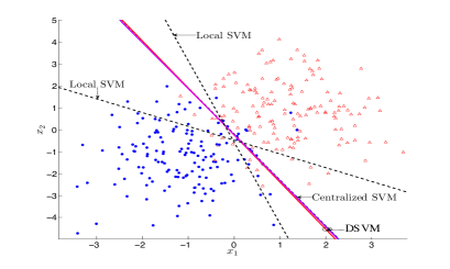
Figure 3: Decision boundary comparison among ADMM-DSVM, centralized SVM and local SVM results for synthetic data generated from two Gaussian classes, and a network of $n=30$ nodes.

To illustrate the performance of the ADMM-DSVM algorithm in pfacgg10jmlr , consider a randomly generated network with $n=30$ nodes. Each node acquires labeled training examples from two different classes, which are equiprobable and consist of random vectors drawn from a two-dimensional (i.e., $p=2$) Gaussian distribution with common covariance matrix $\bm{\Sigma}_{x}=[1,\;0;\;0,\;2]$, and mean vectors ${\mbox{\boldmath$\mu$}}_{1}=[-1,\;-1]^{\top}$ and ${\mbox{\boldmath$\mu$}}_{2}=[1,\;1]^{\top}$, respectively. The Bayes optimal classifier for this 2-class problem is linear (duda, , Ch. 2). To visualize this test case, Fig. 3 depicts the global training set, along with the linear discriminant functions found by the centralized SVM (14) and the ADMM-DSVM at two different nodes after 400 iterations. Local SVM results for two different nodes are also included for comparison. It is apparent that ADMM-DSVM approaches the decision rule of its centralized counterpart, whereas local classifiers deviate since they neglect most of the training examples in the network.

Decentralized Clustering

Unsupervised learning using a network of wireless sensors as an exploratory infrastructure is well motivated for inferring hidden structures in distributed data collected by the sensors. Different from supervised SVM-based classification tasks, each node $i=1,\ldots,n$ has available a set of unlabeled observations ${\mathcal{X}}_{i}:=\{{\mathbf{x}}_{il},\;l=1,\ldots,m_{i}\}$, drawn from a total of $K$ classes. In this network setting, the goal is to design local clustering rules assigning each ${\mathbf{x}}_{il}$ to a cluster $k\in\{1,\ldots,K\}$. Again, the desiderata is a decentralized algorithm capable of attaining the performance of a benchmark clustering scheme, where all $\{{\mathcal{X}}_{i}\}_{i=1}^{n}$ are centrally available for joint processing.

Various criteria are available to quantify similarity among observations in a centralized setting, and a popular selection is the deterministic partitional clustering (DPC) one entailing prototypical elements (a.k.a. cluster centroids) per class in order to avoid comparisons between every pair of observations. Let ${\mbox{\boldmath$\mu$}}_{k}$ denote the prototype element for class $k$, and $\nu_{ilk}$ the membership coefficient of ${\mathbf{x}}_{il}$ to class $k$. A natural clustering problem amounts to specifying the family of $K$ clusters with centroids $\{{\mbox{\boldmath$\mu$}}_{k}\}_{k=1}^{K}$, such that the sum of squared-errors is minimized; that is

$$\min_{\{\nu_{ilk}\in{\mathcal{V}}\},\{{\mbox{\boldmath$\mu$}}_{k}\}}\sum_{i=1}^{n}\sum_{l=1}^{m_{i}}\sum_{k=1}^{K}\nu_{ilk}^{\rho}\left\|{\mathbf{x}}_{il}-{\mbox{\boldmath$\mu$}}_{k}\right\|^{2}$$ (16)

where $\rho\geq 1$ is a tuning parameter, and ${\mathcal{V}}:=\{\nu_{ilk}:\sum_{k}\nu_{ilk}^{\rho}=1,\;\nu_{ilk}\in[0,1],\;\forall i,l\}$ denotes the convex set of constraints on all membership coefficients. With $\rho=1$ and $\{{\mbox{\boldmath$\mu$}}_{k}\}$ fixed, (16) becomes a linear program in $\nu_{ilk}$. Consequently, (16) admits binary $\{0,1\}$ optimal solutions giving rise to the so-termed hard assignments, by choosing the cluster $k$ for ${\mathbf{x}}_{il}$ whenever $\nu_{ilk}=1$. Otherwise, for $\rho>1$ the optimal coefficients generally result in soft membership assignments, and the optimal cluster is $k^{*}:=\arg\max_{k}\nu_{ilk}^{\rho}$ for ${\mathbf{x}}_{il}$. In either case, the DPC clustering problem (16) is NP-hard, which motivates the (suboptimal) K-means algorithm that, on a per iteration basis, proceeds in two-steps to minimize the cost in (16) w.r.t.: (S1) ${\mathcal{V}}$ with $\{{\mbox{\boldmath$\mu$}}_{k}\}$ fixed; and (S2) $\{{\mbox{\boldmath$\mu$}}_{k}\}$ with ${\mathcal{V}}$ fixed lloyd82PCM . Convergence of this two-step alternating-minimization scheme is guaranteed at least to a local minimum. Nonetheless, K-means requires central availability of global information (those variables that are fixed per step), which challenges in-network implementations. For this reason, most early attempts are either confined to specific communication network topologies, or, they offer no closed-form local solutions; see e.g., Nowak03dem ; whk08ICML .

To address these limitations, pfacgg11jstsp casts (16) [yet another instance of (1)] as a decentralized estimation problem. It is thus possible to leverage ADMM iterations and solve (16) in a decentralized fashion through information exchanges among single-hop neighbors only. Albeit the non-convexity of (16), the decentralized DPC iterations in pfacgg11jstsp provably approach a local minimum arbitrarily closely, where the asymptotic convergence holds for hard K-means with $\rho=1$. Further extensions in pfacgg11jstsp include a decentralized expectation-maximization algorithm for probabilistic partitional clustering, and methods to handle unknown number of classes.

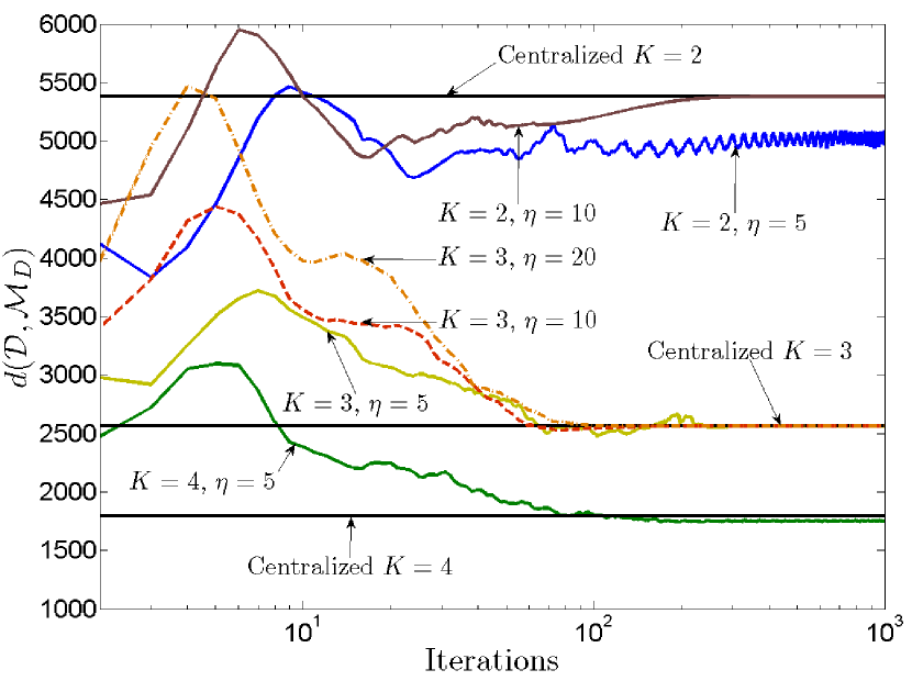
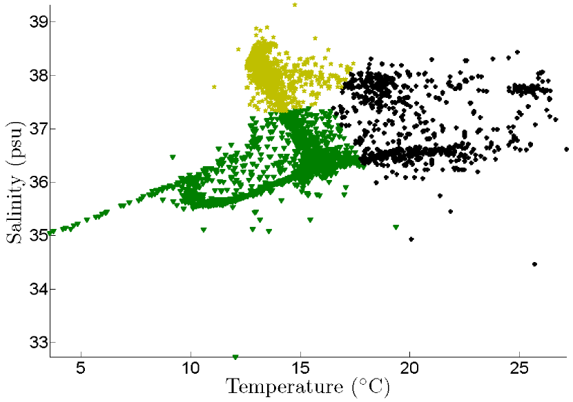
Figure 4: Average performance of hard-DKM on a real data set using a WSN with $n=20$ nodes for various values of $\eta$ and $K$ (left). Clustering with $K=3$ and $\eta=5$ (right) at $k=400$ iterations.

Clustering of oceanographic data. Environmental monitoring is a typical application of WSNs. In WSNs deployed for oceanographic monitoring, the cost of computation per node is lower than the cost of accessing each node’s observations oceansensors . This makes the option of centralized processing less attractive, thus motivating decentralized processing. Here we test the decentralized DPC schemes of pfacgg11jstsp on real data collected by multiple underwater sensors in the Mediterranean coast of Spain WOD , with the goal of identifying regions sharing common physical characteristics. A total of $5,720$ feature vectors were selected, each having entries the temperature (^∘C) and salinity (psu) levels ($p=2$). The measurements were normalized to have zero mean, unit variance, and they were grouped in $n=20$ blocks (one per sensor) of $m_{i}=286$ measurements each. The algebraic connectivity of the WSN is 0.2289 and the average degree per node is 4.9. Fig. 4 (left) shows the performance of 25 Monte Carlo runs for the hard-DKM algorithm with different values of the parameter $c:=\eta$. The best average convergence rate was obtained for $\eta=5$, attaining the average centralized performance after 300 iterations. Tests with different values of $K$ and $\eta$ are also included in Fig. 4 (left) for comparison. Note that for $K=2$ and $\eta=5$ hard-DKM hovers around a point without converging. Choosing a larger $\eta$ guarantees convergence of the algorithm to a unique solution. The clustering results of hard-DKM at $k=400$ iterations for $\eta=5$ and $K=3$ are depicted in Fig. 4 (right).

4 Decentralized Adaptive Estimation

Sections 2 and 3 dealt with decentralized batch estimation, whereby network nodes acquire data only once and then locally exchange messages to reach consensus on the desired estimators. In many applications however, networks are deployed to perform estimation in a constantly changing environment without having available a complete statistical description of the underlying processes of interest, e.g., with time-varying thermal or seismic sources. This motivates the development of decentralized adaptive estimation schemes, where nodes collect data sequentially in time and local estimates are recursively refined “on-the-fly.” In settings where statistical state models are available, it is prudent to develop model-based tracking approaches implementing in-network Kalman or particle filters. Next, Section 2’s scope is broadened to facilitate real-time (adaptive) processing of network data, when the local costs in (1) and unknown parameters are allowed to vary with time.

4.1 Decentralized Least-Mean Squares

A decentralized least-mean squares (LMS) algorithm is developed here for adaptive estimation of (possibly) nonstationary parameters, even when statistical information such as ensemble data covariances are unknown. Suppose network nodes are deployed to estimate a signal vector $\mathbf{s}(t)\in\mathbb{R}^{p\times 1}$ in a collaborative fashion subject to single-hop communication constraints, by resorting to the linear LMS criterion, see e.g., sk95book ; Diffusion_LMS ; SMG_D_LMS . Per time instant $t=0,1,2,\ldots$, each node has available a regression vector $\mathbf{h}_{i}(t)\in\mathbb{R}^{p\times 1}$ and acquires a scalar observation $y_{i}(t)$, both assumed zero-mean without loss of generality. Introducing the global vector $\mathbf{y}(t):=\left[\mathbf{y}_{1}(t)\ldots\mathbf{y}_{n}(t)\right]^{\top}\in\mathbb{R}^{n\times 1}$ and matrix $\mathbf{H}(t):=\left[\mathbf{h}_{1}(t)\ldots\mathbf{h}_{n}(t)\right]^{\top}\in\mathbb{R}^{n\times p}$, the global time-dependent LMS estimator of interest can be written as (sk95book, ; Diffusion_LMS, ; SMG_D_LMS, , p. 14)

$$\hat{\mathbf{s}}(t):=\arg\min_{\mathbf{s}}\mathbb{E}\left[\|{\mathbf{y}}(t)-\mathbf{H}(t)\mathbf{s}\|^{2}\right]={\arg}\min_{\mathbf{s}}\textstyle\sum_{i=1}^{n}\mathbb{E}\left[(y_{i}(t)-\mathbf{h}^{\top}_{i}(t)\mathbf{s})^{2}\right].$$ (17)

For jointly wide-sense stationary $\{\mathbf{x}(t),\mathbf{H}(t)\}$, solving (17) leads to the well-known Wiener filter estimate $\hat{\mathbf{s}}_{W}=\bm{\Sigma}_{H}^{-1}\bm{\Sigma}_{Hy}$, where $\bm{\Sigma}_{H}:=\mathbb{E}[\mathbf{H}^{\top}(t)\mathbf{H}(t)]$ and $\bm{\Sigma}_{Hy}:=\mathbb{E}[\mathbf{H}^{\top}(t)\mathbf{y}(t)]$; see e.g., (sk95book, , p. 15).

For the cases where the auto- and cross-covariance matrices $\bm{\Sigma}_{H}$ and $\bm{\Sigma}_{Hy}$ are unknown, the approach followed here to develop the decentralized (D-) LMS algorithm includes two main building blocks: (i) recast (17) into an equivalent form amenable to in-network processing via the ADMM framework of Section 2; and (ii) leverage stochastic approximation iterations kushner to obtain an adaptive LMS-like algorithm that can handle the unavailability/variation of statistical information. Following those algorithmic construction steps outlined in Section 2, the following updating recursions are obtained for the multipliers $\mathbf{v}_{i}(t)$ and the local estimates $\mathbf{s}_{i}(t+1)$ at time instant $t+1$ and $i=1,\ldots,n$

$$\mathbf{v}_{i}(t) =\mathbf{v}_{i}(t-1)+c\sum_{j\in{\mathcal{N}}_{i}}[\mathbf{s}_{i}(t)-\mathbf{s}_{j}(t)]$$ (18)

$$\mathbf{s}_{i}(t+1) =\arg\min_{\mathbf{s}_{i}}\left\{\mathbb{E}\left[(y_{i}(t+1)-\mathbf{h}^{\top}_{i}(t+1)\mathbf{s}_{i})^{2}\right]+\mathbf{v}_{i}^{\top}(t)\mathbf{s}_{i}\phantom{\sum_{j\in{\cal N}_{i}}}\right.$$

$$\hskip 59.75095pt\left.+c\sum_{j\in{\cal N}_{i}}\left\|\mathbf{s}_{i}-\frac{\mathbf{s}_{i}(t)+\mathbf{s}_{j}(t)}{2}\right\|^{2}\right\}.$$ (19)

It is apparent that after differentiating (19) and setting the gradient equal to zero, $\mathbf{s}_{i}(t+1)$ can be obtained as the root of an equation of the form

$$\mathbb{E}[\bm{\varphi}(\mathbf{s}_{i},y_{i}(t+1),\mathbf{h}_{i}(t+1))]=\mathbf{0}$$ (20)

where $\bm{\varphi}$ corresponds to the stochastic gradient of the cost in (19). However, the previous equation cannot be solved since the nodes do not have available any statistical information about the acquired data. Inspired by stochastic approximation techniques (such as the celebrated Robbins-Monro algorithm; see e.g.,(kushner, , Ch. 1)) which iteratively find the root of (20) given noisy observations $\{\bm{\varphi}(\mathbf{s}_{i}(t),y_{i}(t+1),\mathbf{h}_{i}(t+1))\}_{t=0}^{\infty}$, one can just drop the unknown expected value to obtain the following D-LMS (i.e., stochastic gradient) updates

$$\mathbf{s}_{i}(t+1)=\mathbf{s}_{i}(t)+\mu\left[\mathbf{h}_{i}(t+1)e_{i}(t+1)-\mathbf{v}_{i}(t)-c\sum_{j\in{\cal N}_{i}}[\mathbf{s}_{i}(t)-\mathbf{s}_{j}(t)]\right]$$ (21)

where $\mu$ denotes a constant step-size, and $e_{i}(t+1):=2[y_{i}(t+1)-\mathbf{h}_{i}^{\top}(t+1)\mathbf{s}_{i}(t)]$ is twice the local a priori error.

Recursions (18) and (21) constitute the D-LMS algorithm, which can be viewed as a stochastic-gradient counterpart of D-BLUE in Section 3.1. D-LMS is a pioneering approach for decentralized online learning, which blends for the first time affordable (first-order) stochastic approximation steps with parallel ADMM iterations. The use of a constant step-size $\mu$ endows D-LMS with tracking capabilities. This is desirable in a constantly changing environment, within which e.g., WSNs are envisioned to operate. The D-LMS algorithm is stable and converges even in the presence of inter-node communication noise (see details in SMG_D_LMS ; MSG_D_LMS ). Further, closed-form expressions for the evolution and the steady-state mean-square error (MSE), as well as selection guidelines for the step-size $\mu$ can be found in MSG_D_LMS .

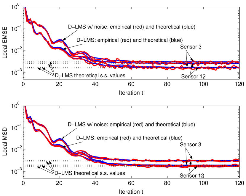
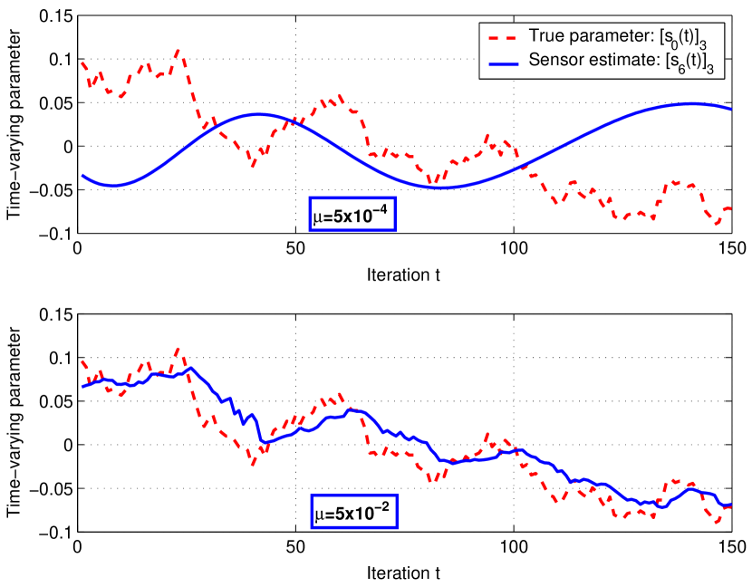
Figure 5: Tracking with D-LMS. (left) Local MSE performance metrics both with and without inter-node communication noise for sensors 3 and 12; and (right) True and estimated time-varying parameters for a representative node, using slow and optimal adaptation levels.

Here we test the tracking performance of D-LMS with a computer simulation. For a random geometric graph with $n=20$ nodes, network-wide observations $y_{i}$ are linearly related to a large-amplitude slowly time-varying parameter vector ${\mathbf{s}}_{0}(t)\in\mathbb{R}^{4}$. Specifically, ${\mathbf{s}}_{0}(t)=\bm{\Theta}{\mathbf{s}}_{0}(t-1)+\bm{\zeta}(t)$, where $\bm{\Theta}=(1-10^{-4})\textrm{diag}(\theta_{1},\ldots,\theta_{p})$ with $\theta_{i}\sim\mathcal{U}[0,1]$. The driving noise is normally distributed with $\bm{\Sigma}_{\zeta}=10^{-4}{\mathbf{I}}_{p}$. To model noisy links, additive white Gaussian noise with variance $10^{-2}$ is present at the receiving end. For $\mu=5\times 10^{-2}$, Fig. 5 (left) depicts the local performance of two representative nodes through the evolution of the excess mean-square error $\textrm{EMSE}_{i}(t)=\mathbb{E}[({\mathbf{h}}_{i}^{\top}(t)[{\mathbf{s}}_{i}(t-1)-{\mathbf{s}}_{0}(t-1)])^{2}]$ and the mean-square deviation $\textrm{MSD}_{i}(t)=\mathbb{E}[\|{\mathbf{s}}_{i}(t)-{\mathbf{s}}_{0}(t)\|^{2}]$ figures of merit. Both noisy and ideal links are considered, and the empirical curves closely follow the theoretical trajectories derived in MSG_D_LMS . Steady-state limiting values are also extremely accurate. As intuitively expected and suggested by the analysis, a performance penalty due to non-ideal links is also apparent. Fig. 5 (right) illustrates how the adaptation level affects the resulting per-node estimates when tracking time-varying parameters with D-LMS. For $\mu=5\times 10^{-4}$ (slow adaptation) and $\mu=5\times 10^{-2}$ (near optimal adaptation), we depict the third entry of the parameter vector $[{\mathbf{s}}_{0}(t)]_{3}$ and the respective estimates from the randomly chosen sixth node. Under optimal adaptation the local estimate closely tracks the true variations, while – as expected – for the smaller step-size D-LMS fails to provide an accurate estimate MSG_D_LMS ; sk95book .

4.2 Decentralized Recursive Least-Squares

The recursive least-squares (RLS) algorithm has well-appreciated merits for reducing complexity and storage requirements, in online estimation of stationary signals, as well as for tracking slowly-varying nonstationary processes sk95book ; Estimation_Theory . RLS is especially attractive when the state and/or data model are not available (as with LMS), and fast convergence rates are at a premium. Compared to the LMS scheme, RLS typically offers faster convergence and improved estimation performance at the cost of higher computational complexity. To enable these valuable tradeoffs in the context of in-network processing, the ADMM framework of Section 2 is utilized here to derive a decentralized (D-) RLS adaptive scheme that can be employed for distributed localization and power spectrum estimation (see also MSG_D_RLS ; MG_D_RLS for further details on the algorithmic construction and convergence claims).

Consider the data setting and linear regression task in Section 4.1. The RLS estimator for the unknown parameter $\mathbf{s}_{0}(t)$ minimizes the exponentially weighted least-squares (EWLS) cost, see e.g., sk95book ; Estimation_Theory

$$\hat{\mathbf{s}}_{\textrm{ewls}}(t):={\arg}\min_{\mathbf{s}}\sum_{\tau=0}^{t}\sum_{i=1}^{n}\gamma^{t-\tau}\left[y_{i}(\tau)-\mathbf{h}^{\top}_{i}(\tau)\mathbf{s}\right]^{2}+\gamma^{t}\mathbf{s}^{T}\bm{\Phi}_{0}\mathbf{s}$$ (22)

where $\gamma\in(0,1]$ is a forgetting factor, while the positive definite matrix $\bm{\Phi}_{0}$ is included for regularization. Note that in forming the EWLS estimator at time $t$, the entire history of data $\{y_{i}(\tau),\mathbf{h}_{i}(\tau)\}_{\tau=0}^{t}$ for $i=1,\ldots,n$ is incorporated in the online estimation process. Whenever $\gamma<1$, past data are exponentially discarded thus enabling tracking of nonstationary processes.

Again to decompose the cost function in (22), in which summands are coupled through the global variable $\mathbf{s}$, we introduce auxiliary variables $\{\mathbf{s}_{i}\}_{i=1}^{n}$ that represent local estimates per node $i$. These local estimates are utilized to form the convex constrained and separable minimization problem in (2), which can be solved using ADMM to yield the following decentralized iterations (details in MSG_D_RLS ; MG_D_RLS )

$$\mathbf{v}_{i}(t) =\mathbf{v}_{i}(t-1)+c\sum_{j\in{\mathcal{N}}_{i}}[\mathbf{s}_{i}(t)-\mathbf{s}_{j}(t)]$$ (23)

$$\mathbf{s}_{i}(t+1) =\bm{\Phi}_{i}^{-1}(t+1)\bm{\psi}_{i}(t+1)-\frac{1}{2}\bm{\Phi}_{i}^{-1}(t+1)\mathbf{v}_{i}(t)$$ (24)

where $\bm{\Phi}_{i}(t+1):=\sum_{\tau=0}^{t+1}\gamma^{t+1-\tau}\mathbf{h}_{i}(\tau)\mathbf{h}_{i}^{\top}(\tau)+n^{-1}\gamma^{t+1}\bm{\Phi}_{0}$ and

$$\bm{\Phi}_{i}^{-1}(t+1) =\gamma^{-1}\bm{\Phi}_{i}^{-1}(t)-\frac{\gamma^{-1}\bm{\Phi}_{i}^{-1}(t){\mathbf{h}}_{i}(t+1){\mathbf{h}}_{i}^{\top}(t+1)\bm{\Phi}_{i}^{-1}(t)}{\gamma+{\mathbf{h}}_{i}^{\top}(t+1)\bm{\Phi}_{i}^{-1}(t){\mathbf{h}}_{i}(t+1)}$$ (25)

$$\bm{\psi}_{i}(t+1) :=\sum_{\tau=0}^{t+1}\gamma^{t+1-\tau}\mathbf{h}_{i}(\tau)y_{i}(\tau)=\gamma\bm{\psi}_{i}(t)+\mathbf{h}_{i}(t+1)y_{i}(t+1).$$ (26)

The D-RLS recursions (23) and (24) involve similar inter-node communication exchanges as in D-LMS. It is recommended to initialize the matrix recursion with $\bm{\Phi}_{i}^{-1}(0)=n\bm{\Phi}_{0}^{-1}:=\delta{\mathbf{I}}_{p}$, where $\delta>0$ is chosen sufficiently large sk95book . The local estimates in D-RLS converge in the mean-sense to the true $\mathbf{s}_{0}$ (time-invariant case), even when information exchanges are imperfect. Closed-form expressions for the bounded estimation MSE along with numerical tests and comparisons with the incremental RLS inc_RLS and diffusion RLS Diffusion_RLS algorithms can be found in MG_D_RLS .

Decentralized spectrum sensing using WSNs. A WSN application where the need for linear regression arises, is spectrum estimation for the purpose of environmental monitoring. Suppose sensors comprising a WSN deployed over some area of interest observe a narrowband source to determine its spectral peaks. These peaks can reveal hidden periodicities due to e.g., a natural heat or seismic source. The source of interest propagates through multi-path channels and is contaminated with additive noise present at the sensors. The unknown source-sensor channels may introduce deep fades at the frequency band occupied by the source. Thus, having each sensor operating on its own may lead to faulty assessments. The available spatial diversity to effect improved spectral estimates, can only be achieved via sensor collaboration as in the decentralized estimation algorithms presented in this chapter.

Let ${\theta}(t)$ denote the evolution of the source signal in time, and suppose that ${\theta}(t)$ can be modeled as an autoregressive (AR) process (Stoica_Book, , p. 106)

$${\theta}(t)=-\sum_{\tau=1}^{p}\alpha_{\tau}{\theta}(t-\tau)+w(t)$$

where $p$ is the order of the AR process, while $\{\alpha_{\tau}\}$ are the AR coefficients and $w(t)$ denotes driving white noise. The source propagates to sensor $i$ via a channel modeled as an FIR filter $C_{i}(z)=\sum_{l=0}^{L_{i}-1}c_{il}z^{-l}$, of unknown order $L_{i}$ and tap coefficients $\{c_{il}\}$ and is contaminated with additive sensing noise $\bar{\epsilon}_{i}(t)$ to yield the observation

$$y_{i}(t)=\sum_{l=0}^{L_{i}-1}c_{il}\theta(t-l)+\bar{\epsilon}_{i}(t).$$

Since $y_{i}(t)$ is an autoregressive moving average (ARMA) process, then Stoica_Book

$$y_{i}(t)=-\sum_{\tau=1}^{p}\alpha_{\tau}y_{i}(t-\tau)+\sum_{\tau^{\prime}=1}^{m}\beta_{\tau^{\prime}}\tilde{\eta}_{i}(t-\tau^{\prime})$$ (27)

where the MA coefficients $\{\beta_{\tau^{\prime}}\}$ and the variance of the white noise process $\tilde{\eta}_{i}(t)$ depend on $\{c_{il}\}$, $\{\alpha_{\tau}\}$ and the variance of the noise terms $w(t)$ and $\bar{\epsilon}_{i}(t)$. For the purpose of determining spectral peaks, the MA term in (27) can be treated as observation noise, i.e., $\epsilon_{i}(t):=\sum_{\tau^{\prime}=1}^{m}\beta_{\tau^{\prime}}\tilde{\eta}_{i}(t-\tau^{\prime})$. This is very important since this way sensors do not have to know the source-sensor channel coefficients as well as the noise variances. Accordingly, the spectral content of the source can be estimated provided sensors estimate the coefficients $\{\alpha_{\tau}\}$. To this end, let ${\mathbf{s}}_{0}:=[\alpha_{1}\ldots\alpha_{p}]^{\top}$ be the unknown parameter of interest. From (27) the regression vectors are given as ${\mathbf{h}}_{i}(t)=[-y_{i}(t-1)\ldots-y_{i}(t-p)]^{\top}$, and can be acquired directly from the sensor measurements $\{y_{i}(t)\}$ without the need of training/estimation.

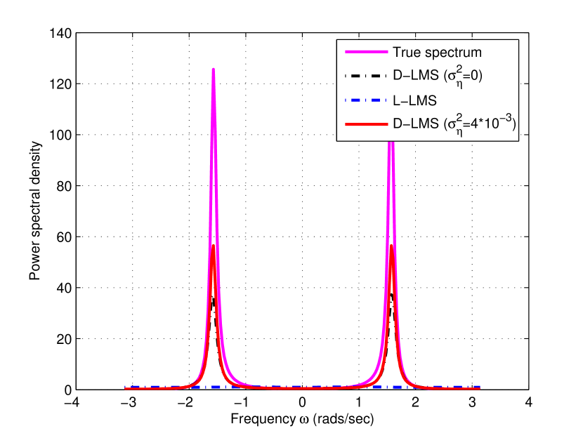
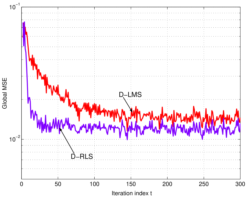
Figure 6: D-LMS in a power spectrum estimation task. (left) The true narrowband spectra is compared to the estimated PSD, obtained after the WSN runs the D-LMS and (non-cooperative) L-LMS algorithms. The reconstruction results correspond to a sensor whose multipath channel from the source introduces a null at $\omega=\pi/2=1.57$. (right) Global MSE evolution (network learning curve) for the D-LMS and D-RLS algorithms.

Performance of the decentralized adaptive algorithms described so far is illustrated next, when applied to the aforementioned power spectrum estimation task. For the numerical experiments, an ad hoc WSN with $n=80$ sensors is simulated as a realization of a random geometric graph. The source-sensor channels corresponding to a few of the sensors are set so that they have a null at the frequency where the AR source has a peak, namely at $\omega=\pi/2$. Fig. 6 (left) depicts the actual power spectral density (PSD) of the source as well as the estimated PSDs for one of the sensors affected by a bad channel. To form the desired estimates in a distributed fashion, the WSN runs the local (L-) LMS and the D-LMS algorithm outlined in Section 4.1. The L-LMS is a non-cooperative scheme since each sensor, say the $i$th, independently runs an LMS adaptive filter fed by its local data $\{y_{i}(t),{\mathbf{h}}_{i}(t)\}$ only. The experiment involving D-LMS is performed under ideal and noisy inter-sensor links. Clearly, even in the presence of communication noise D-LMS exploits the spatial diversity available and allows all sensors to estimate accurately the actual spectral peak, whereas L-LMS leads the problematic sensors to misleading estimates.

For the same setup, Fig. 6 (right) shows the global learning curve evolution $\textrm{MSE}(t)=(1/n)\sum_{i=1}^{n}\|y_{i}(t)-{\mathbf{h}}_{i}^{\top}(t){\mathbf{s}}_{i}(t-1)\|^{2}$. The D-LMS and the D-RLS algorithms are compared under ideal communication links. It is apparent that D-RLS achieves improved performance both in terms of convergence rate and steady state MSE. As discussed in Section 4.2 this comes at the price of increased computational complexity per sensor, while the communication costs incurred are identical.

4.3 Decentralized Model-based Tracking

The decentralized adaptive schemes in Secs. 4.1 and 4.2 are suitable for tracking slowly time-varying signals in settings where no statistical models are available. In certain cases, such as target tracking, state evolution models can be derived and employed by exploiting the physics of the problem. The availability of such models paves the way for improved state tracking via Kalman filtering/smoothing techniques, e.g., see Opt_Filtering_Moore ; Estimation_Theory . Model-based decentralized Kalman filtering/smoothing as well as particle filtering schemes for multi-node networks are briefly outlined here.

Initial attempts to distribute the centralized KF recursions (see Olfati_Kalman and references in sgrr08tsp ) rely on consensus-averaging Consensus_Averaging . The idea is to estimate across nodes those sufficient statistics (that are expressible in terms of network-wide averages) required to form the corrected state and corresponding corrected state error covariance matrix. Clearly, there is an inherent delay in obtaining these estimates confining the operation of such schemes only to applications with slow-varying state vectors $\mathbf{s}_{0}(t)$, and/or fast communications needed to complete multiple consensus iterations within the time interval separating the acquisition of consecutive measurements $y_{i}(t)$ and $y_{i}(t+1)$. Other issues that may lead to instability in existing decentralized KF approaches are detailed in sgrr08tsp .

Instead of filtering, the delay incurred by those inner-loop consensus iterations motivated the consideration of fixed-lag decentralized Kalman smoothing (KS) in sgrr08tsp . Matching consensus iterations with those time instants of data acquisition, fixed-lag smoothers allow sensors to form local MMSE optimal smoothed estimates, which take advantage of all acquired measurements within the “waiting period.” The ADMM-enabled decentralized KS in sgrr08tsp also overcomes the noise-related limitations of consensus-averaging algorithms xbk07jpdc . In the presence of communication noise, these estimates converge in the mean sense, while their noise-induced variance remains bounded. This noise resiliency allows sensors to exchange quantized data further lowering communication cost. For a tutorial treatment of decentralized Kalman filtering approaches using WSNs (including the decentralized ADMM-based KS of sgrr08tsp and strategies to reduce the communication cost of state estimation problems), the interested reader is referred to dkf_control_mag . These reduced-cost strategies exploit the redundancy in information provided by individual observations collected at different sensors, different observations collected at different sensors, and different observations acquired at the same sensor.

On a related note, a collaborative algorithm is developed in cg_cartography to estimate the channel gains of wireless links in a geographical area. Kriged Kalman filtering (KKF) ripley , which is a tool with widely appreciated merits in spatial statistics and geosciences, is adopted and implemented in a decentralized fashion leveraging the ADMM framework described here. The distributed KKF algorithm requires only local message passing to track the time-variant so-termed “shadowing field” using a network of radiometers, yet it provides a global view of the radio frequency (RF) environment through consensus iterations; see also Section 5.3 for further elaboration on spectrum sensing carried out via wireless cognitive radio networks.

To wrap-up the discussion, consider a network of collaborating agents (e.g., robots) equipped with wireless sensors measuring distance and/or bearing from a target that they wish to track. Even if state models are available, the nonlinearities present in these measurements prevent sensors from employing the clairvoyant (linear) Kalman tracker discussed so far. In response to these challenges, dpf develops a set-membership constrained particle filter (PF) approach that: (i) exhibits performance comparable to the centralized PF; (ii) requires only communication of particle weights among neighboring sensors; and (iii) it can afford both consensus-based and incremental averaging implementations. Affordable inter-sensor communications are enabled through a novel distributed adaptation scheme, which considerably reduces the number of particles needed to achieve a given performance. The interested reader is referred to dpf_tutorial for a recent tutorial account of decentralized PF in multi-agent networks.

5 Decentralized Sparsity-regularized Rank Minimization

Modern network data sets typically involve a large number of attributes. This fact motivates predictive models offering a sparse, broadly meaning parsimonious, representation in terms of a few attributes. Such low-dimensional models facilitate interpretability and enhanced predictive performance. In this context, this section deals with ADMM-based decentralized algorithms for sparsity-regularized rank minimization. It is argued that such algorithms are key to unveiling Internet traffic anomalies given ubiquitous link-load measurements. Moreover, the notion of RF cartography is subsequently introduced to exemplify the development of a paradigm infrastructure for situational awareness at the physical layer of wireless cognitive radio (CR) networks. A (subsumed) decentralized sparse linear regression algorithm is outlined to accomplish the aforementioned cartography task.

5.1 Network Anomaly Detection Via Sparsity and Low Rank

Consider a backbone IP network, whose abstraction is a graph with $n$ nodes (routers) and $L$ physical links. The operational goal of the network is to transport a set of $F$ origin-destination (OD) traffic flows associated with specific OD (ingress-egress router) pairs. Let $x_{l,t}$ denote the traffic volume (in bytes or packets) passing through link $l\in\{1,\ldots,L\}$ over a fixed time interval $(t,t+\Delta t)$. Link counts across the entire network are collected in the vector ${\bf x}_{t}\in\mathbb{R}^{L}$, e.g., using the ubiquitous SNMP protocol. Single-path routing is adopted here, meaning a given flow’s traffic is carried through multiple links connecting the corresponding source-destination pair along a single path. Accordingly, over a discrete time horizon $t\in[1,T]$ the measured link counts ${\bf X}:=[x_{l,t}]\in\mathbb{R}^{L\times T}$ and (unobservable) OD flow traffic matrix ${\bf Z}:=[z_{f,t}]\in\mathbb{R}^{F\times T}$, are thus related through ${\bf X}={\bf R}{\bf Z}$ lakhina , where the so-termed routing matrix ${\bf R}:=[r_{l,f}]\in\{0,1\}^{L\times F}$ is such that $r_{l,f}=1$ if link $l$ carries the flow $f$, and zero otherwise. The routing matrix is ‘wide,’ as for backbone networks the number of OD flows is much larger than the number of physical links $(F\gg L)$. A cardinal property of the traffic matrix is noteworthy. Common temporal patterns across OD traffic flows in addition to their almost periodic behavior, render most rows (respectively columns) of the traffic matrix linearly dependent, and thus ${\bf Z}$ typically has low rank. This intuitive property has been extensively validated with real network data; see Fig. 7 and e.g., lakhina .

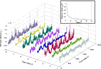
Figure 7: Volumes of $6$ representative (out of $121$ total) OD flows, taken from the operation of Internet-2 during a seven-day period. Temporal periodicities and correlations across flows are apparent. As expected, in this case ${\bf Z}$ can be well approximated by a low-rank matrix, since its normalized singular values decay rapidly to zero.

It is not uncommon for some of the OD flow rates to experience unexpected abrupt changes. These so-termed traffic volume anomalies are typically due to (unintentional) network equipment misconfiguration or outright failure, unforeseen behaviors following routing policy modifications, or, cyber attacks (e.g., DoS attacks) which aim at compromising the services offered by the network zggr05 ; lakhina ; mrspmag13 . Let $a_{f,t}$ denote the unknown amount of anomalous traffic in flow $f$ at time $t$, which one wishes to estimate. Explicitly accounting for the presence of anomalous flows, the measured traffic carried by link $l$ is then given by $y_{l,t}=\sum_{f}r_{l,f}(z_{f,t}+a_{f,t})+\epsilon_{l,t},~{}t=1,...,T$, where the noise variables $\epsilon_{l,t}$ capture measurement errors and unmodeled dynamics. Traffic volume anomalies are (unsigned) sudden changes in the traffic of OD flows, and as such their effect can span multiple links in the network. A key difficulty in unveiling anomalies from link-level measurements only is that oftentimes, clearly discernible anomalous spikes in the flow traffic can be masked through “destructive interference” of the superimposed OD flows lakhina . An additional challenge stems from missing link-level measurements $y_{l,t}$, an unavoidable operational reality affecting most traffic engineering tasks that rely on (indirect) measurement of traffic matrices Roughan . To model missing link measurements, collect the tuples $(l,t)$ associated with the available observations $y_{l,t}$ in the set $\Omega\subseteq[1,2,...,L]\times[1,2,...,T]$. Introducing the matrices ${\bf Y}:=[y_{l,t}],{\bf E}:=[\epsilon_{l,t}]\in\mathbb{R}^{L\times T}$, and ${\bf A}:=[a_{f,t}]\in\mathbb{R}^{F\times T}$, the (possibly incomplete) set of link-traffic measurements can be expressed in compact matrix form as

$$\mathcal{P}_{\Omega}({\bf Y})=\mathcal{P}_{\Omega}({\bf X}+{\bf R}{\bf A}+{\bf E})$$ (28)

where the sampling operator $\mathcal{P}_{\Omega}(.)$ sets the entries of its matrix argument not in $\Omega$ to zero, and keeps the rest unchanged. Since the objective here is not to estimate the OD flow traffic matrix ${\bf Z}$, (28) is expressed in terms of the nominal (anomaly-free) link-level traffic rates ${\bf X}:={\bf R}{\bf Z}$, which inherits the low-rank property of ${\bf Z}$. Anomalies in ${\bf A}$ are expected to occur sporadically over time, and last for a short time relative to the (possibly long) measurement interval $[1,T]$. In addition, only a small fraction of the flows is supposed to be anomalous at a any given time instant. This renders the anomaly matrix ${\bf A}$ sparse across rows (flows) and columns (time).

Recently, a natural estimator leveraging the low rank property of ${\bf X}$ and the sparsity of ${\bf A}$ was put forth in mmg13tsp , which can be found at the crossroads of compressive sampling Do06CS and timely low-rank plus sparse matrix decompositions CLMW09 ; CSPW11 . The idea is to fit the incomplete data $\mathcal{P}_{\Omega}({\bf Y})$ to the model ${\bf X}+{\bf R}{\bf A}$ [cf. (28)] in the LS error sense, as well as minimize the rank of ${\bf X}$, and the number of nonzero entries of ${\bf A}$ measured by its $\ell_{0}$-(pseudo) norm. Unfortunately, albeit natural both rank and $\ell_{0}$-norm criteria are in general NP-hard to optimize. Typically, the nuclear norm $\|{\bf X}\|_{*}:=\sum_{k}\sigma_{k}({\bf X})$ ($\sigma_{k}({\bf X})$ denotes the $k$-th singular value of ${\bf X}$) and the $\ell_{1}$-norm $\|{\bf A}\|_{1}$ are adopted as surrogates F02 ; CT05 , since they are the closest convex approximants to $\textrm{rank}({\bf X})$ and $\|{\bf A}\|_{0}$, respectively. Accordingly, one solves

$$\min_{\{{\bf X},{\bf A}\}}\|\mathcal{P}_{\Omega}({\bf Y}-{\bf X}-{\bf R}{\bf A})\|_{F}^{2}+\lambda_{\ast}\|{\bf X}\|_{*}+\lambda_{1}\|{\bf A}\|_{1}$$ (29)

where $\lambda_{*},\lambda_{1}\geq 0$ are rank- and sparsity-controlling parameters. While a non-smooth optimization problem, (29) is appealing because it is convex. An efficient accelerated proximal gradient algorithm with quantifiable iteration complexity was developed to unveil network anomalies tit_recovery_2012 . Interestingly, (29) also offers a cleansed estimate of the link-level traffic $\hat{{\bf X}}$, that could be subsequently utilized for network tomography tasks. In addition, (29) jointly exploits the spatio-temporal correlations in link traffic as well as the sparsity of anomalies, through an optimal single-shot estimation-detection procedure that turns out to outperform the algorithms in lakhina and zggr05 (the latter decouple the estimation and detection steps); see Fig. 8.

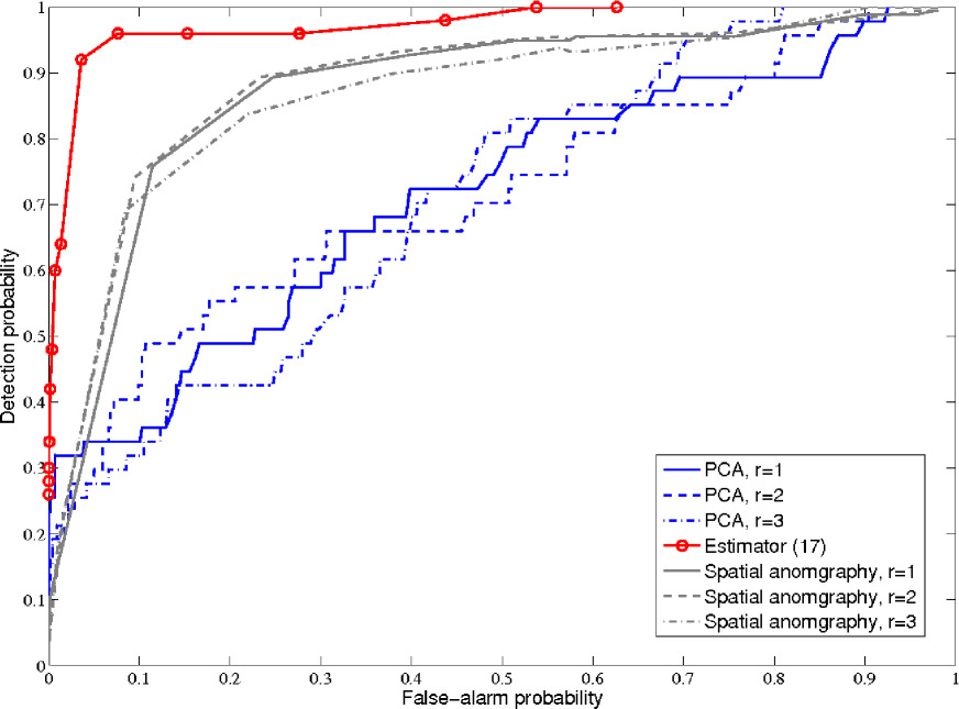
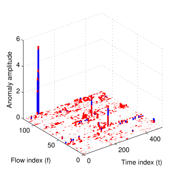
Figure 8: Unveiling anomalies from Internet-2 data. (Left) ROC curve comparison between (29) and the PCA methods in lakhina ; zggr05 , for different values of the $\text{rank}({\mathbf{Z}})$. Leveraging sparsity and low rank jointly leads to improved performance. (Right) In red, the estimated anomaly map $\hat{{\bf A}}$ obtained via (29) superimposed to the “true” anomalies shown in blue mmg13jstsp .

5.2 In-network Traffic Anomaly Detection

Implementing (29) presumes that network nodes continuously communicate their link traffic measurements to a central monitoring station, which uses their aggregation in $\mathcal{P}_{\Omega}({\bf Y})$ to unveil anomalies. While for the most part this is the prevailing operational paradigm adopted in current networks, it is prudent to reflect on the limitations associated with this architecture. For instance, fusing all this information may entail excessive protocol overheads. Moreover, minimizing the exchanges of raw measurements may be desirable to reduce unavoidable communication errors that translate to missing data. Solving (29) centrally raises robustness concerns as well, since the central monitoring station represents an isolated point of failure.

These reasons prompt one to develop fully-decentralized iterative algorithms for unveiling traffic anomalies, and thus embed network anomaly detection functionality to the routers. As in Section 2, per iteration node $i$ carries out simple computational tasks locally, relying on its own link count measurements (a submatrix ${\bf Y}_{i}$ within ${\bf Y}:=[{\bf Y}_{1}^{\top},\ldots,{\bf Y}_{n}^{\top}]^{\top}$ corresponding to router $i$’s links). Subsequently, local estimates are refined after exchanging messages only with directly connected neighbors, which facilitates percolation of local information to the whole network. The end goal is for network nodes to consent on a global map of network anomalies $\hat{{\bf A}}$, and attain (or at least come close to) the estimation performance of the centralized counterpart (29) which has all data $\mathcal{P}_{\Omega}({\bf Y})$ available.

Problem (29) is not amenable to distributed implementation because of the non-separable nuclear norm present in the cost function. If an upper bound $\textrm{rank}(\hat{\bf X})\leq\rho$ is a priori available [recall $\hat{\bf X}$ is the estimated link-level traffic obtained via (29)], the search space of (29) is effectively reduced, and one can factorize the decision variable as ${\bf X}={\bf P}{\bf Q}^{\top}$, where ${\bf P}$ and ${\bf Q}$ are $L\times\rho$ and $T\times\rho$ matrices, respectively. Again, it is possible to interpret the columns of ${\bf X}$ (viewed as points in $\mathbb{R}^{L}$) as belonging to a low-rank nominal subspace, spanned by the columns of ${\bf P}$. The rows of ${\bf Q}$ are thus the projections of the columns of ${\bf X}$ onto the traffic subspace. Next, consider the following alternative characterization of the nuclear norm (see e.g. srebro_2005 )

$$\|{\bf X}\|_{*}:=\min_{\{{\bf P},{\bf Q}\}}~{}~{}~{}\frac{1}{2}\left(\|{\bf P}\|_{F}^{2}+\|{\bf Q}\|_{F}^{2}\right),\quad\text{s. to}~{}~{}~{}{\bf X}={\bf P}{\bf Q}^{\top}$$ (30)

where the optimization is over all possible bilinear factorizations of ${\bf X}$, so that the number of columns $\rho$ of ${\bf P}$ and $\mathbf{Q}$ is also a variable. Leveraging (30), the following reformulation of (29) provides an important first step towards obtaining a decentralized algorithm for anomaly identification

$$\min_{\{{\bf P},{\bf Q},{\bf A}\}}\sum_{i=1}^{n}\left[\|\mathcal{P}_{\Omega_{i}}({\bf Y}_{i}-{\bf P}_{i}{\bf Q}^{\top}-{\bf R}_{i}{\bf A})\|_{F}^{2}+\frac{\lambda_{*}}{2n}\left(n\|{\bf P}_{i}\|_{F}^{2}+\|{\bf Q}\|_{F}^{2}\right)+\frac{\lambda_{1}}{n}\|{\bf A}\|_{1}\right]$$ (31)

which is non-convex due to the bilinear terms ${\bf P}_{i}{\bf Q}^{\top}$, and where ${\bf R}:=\left[{\bf R}_{1}^{\top},\ldots,{\bf R}_{n}^{\top}\right]^{\top}$ is partitioned into local routing tables available per router $i$. Adopting the separable Frobenius-norm regularization in (31) comes with no loss of optimality relative to (29), provided $\textrm{rank}(\hat{\bf X})\leq\rho$. By finding the global minimum of (31) [which could entail considerably less variables than (29)], one can recover the optimal solution of (29). But since (31) is non-convex, it may have stationary points which need not be globally optimum. As asserted in (mmg13tsp, , Prop. 1) however, if a stationary point $\{\bar{{\bf P}},\bar{{\bf Q}},\bar{{\bf A}}\}$ of (31) satisfies $\|\mathcal{P}_{\Omega}({\bf Y}-\bar{{\bf P}}\bar{{\bf Q}}^{\top}-\bar{{\bf A}})\|<\lambda_{*}$, then $\{\hat{\bf X}:=\bar{{\bf P}}\bar{{\bf Q}}^{\top},\hat{{\bf A}}:=\bar{{\bf A}}\}$ is the globally optimal solution of (29).

To decompose the cost in (31), in which summands inside the square brackets are coupled through the global variables $\{{\bf Q},{\bf A}\}$, one can proceed as in Section 2 and introduce auxiliary copies $\{{\bf Q}_{i},{\bf A}_{i}\}_{i=1}^{n}$ representing local estimates of $\{{\bf Q},{\bf A}\}$, one per node $i$. These local copies along with consensus constraints yield the decentralized estimator

$$\min_{\{{\bf P}_{i},{\bf Q}_{i},{\bf A}_{i}\}} \sum_{i=1}^{n}\left[\|\mathcal{P}_{\Omega_{i}}({\bf Y}_{i}-{\bf P}_{i}{\bf Q}_{i}^{\top}-{\bf R}_{i}{\bf A}_{i})\|_{F}^{2}+\frac{\lambda_{*}}{2n}\left(n\|{\bf P}_{i}\|_{F}^{2}+\|{\bf Q}_{i}\|_{F}^{2}\right)+\frac{\lambda_{1}}{n}\|{\bf A}_{i}\|_{1}\right]$$ (32)

s. to $$\quad{\bf Q}_{i}={\bf Q}_{j},\>\>{\bf A}_{i}={\bf A}_{j},\;\;i=1,\ldots,n,\;\;j\in{\cal N}_{i},\;\;i\neq j$$

which follows the general form in (2), and is equivalent to (31) provided the network topology graph is connected. Even though consensus is a fortiori imposed within neighborhoods, it carries over to the entire (connected) network and local estimates agree on the global solution of (31). Exploiting the separable structure of (32) using the ADMM, a general framework for in-network sparsity-regularized rank minimization was put forth in mmg13tsp . In a nutshell, local tasks per iteration $k=1,2,\ldots$ entail solving small unconstrained quadratic programs to refine the normal subspace ${\bf P}_{i}[k]$, in addition to soft-thresholding operations to update the anomaly maps ${\bf A}_{i}[k]$ per router. Routers exchange their estimates $\{{\bf Q}_{i}[k],{\bf A}_{i}[k]\}$ only with directly connected neighbors per iteration. This way the communication overhead remains affordable, regardless of the network size $n$.

When employed to solve non-convex problems such as (32), so far ADMM offers no convergence guarantees. However, there is ample experimental evidence in the literature that supports empirical convergence of ADMM, especially when the non-convex problem at hand exhibits “favorable” structure Boyd_ADMM . For instance, (32) is a linearly constrained bi-convex problem with potentially good convergence properties – extensive numerical tests in mmg13tsp demonstrate that this is indeed the case. While establishing convergence remains an open problem, one can still prove that upon convergence the distributed iterations attain consensus and global optimality, thus offering the desirable centralized performance guarantees mmg13tsp .

5.3 RF Cartography Via Decentralized Sparse Linear Regression

In the domain of spectrum sensing for CR networks, RF cartography amounts to constructing in a distributed fashion: i) global power spectral density (PSD) maps capturing the distribution of radiated power across space, time, and frequency; and ii) local channel gain (CG) maps offering the propagation medium per frequency from each node to any point in space cg_cartography . These maps enable identification of opportunistically available spectrum bands for re-use and handoff operation; as well as localization, transmit-power estimation, and tracking of primary user activities. While the focus here is on the construction of PSD maps, the interested reader is referred to tut_rf_cartog for a tutorial treatment on CG cartography.

A cooperative approach to RF cartography was introduced in bazerque , that builds on a basis expansion model of the PSD map $\Phi({\mathbf{x}},f)$ across space ${\mathbf{x}}\in\mathbb{R}^{2}$, and frequency $f$. Spatially-distributed CRs collect smoothed periodogram samples of the received signal at given sampling frequencies, based on which the unknown expansion coefficients are determined. Introducing a virtual spatial grid of candidate source locations, the estimation task can be cast as a linear LS problem with an augmented vector of unknown parameters. Still, the problem complexity (or effective degrees of freedom) can be controlled by capitalizing on two forms of sparsity: the first one introduced by the narrow-band nature of transmit-PSDs relative to the broad swaths of usable spectrum; and the second one emerging from sparsely located active radios in the operational space (due to the grid artifact). Nonzero entries in the parameter vector sought correspond to spatial location-frequency band pairs corresponding to active transmissions. All in all, estimating the PSD map and locating the active transmitters as a byproduct boils down to a variable selection problem. This motivates well employment of the ADMM and the least-absolute shrinkage and selection operator (Lasso) for decentralized sparse linear regression mateos_dlasso ; mmg13tsp , an estimator subsumed by (29) when ${\bf X}=\mathbf{0}_{L\times T}$, $T=1$, and matrix ${\bf R}$ has a specific structure that depends on the chosen bases and the path-loss propagation model.

Sparse total LS variants are also available to cope with uncertainty in the regression matrix, arising due to inaccurate channel estimation and grid-mismatch effects tut_rf_cartog . Nonparametric spline-based PSD map estimators rf_splines have been also shown effective in capturing general propagation characteristics including both shadowing and fading; see also Fig. 9 for an actual PSD atlas spanning $14$ frequency sub-bands.

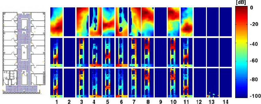
Figure 9: Spline-based RF cartography from real wireless LAN data. (Left) Detailed floor plan schematic including the location of $N=166$ sensing radios; (Right-bottom) original measurements spanning $14$ frequency sub-bands; (Right-center) estimated maps over the surveyed area; and (Right-top) extrapolated maps. The proposed decentralized estimator is capable of recovering the $9$ (out of $14$ total) center frequencies that are being utilized for transmission. It accurately recovers the power levels in the surveyed area with a smooth extrapolation to zones were there are no measurements, and suggests possible locations for the transmitters rf_splines .

6 Convergence Analysis

In this section we analyze the convergence and assess the rate of convergence for the decentralized ADMM algorithm outlined in Section 2. We focus on the batch learning setup, where the local cost functions are static.

6.1 Preliminaries

Network model revisitied and elements of algebraic graph theory. Recall the network model briefly introduced in Section 1, based on a connected graph composed of a set of $n$ nodes (agents, vertices), and a set of $L$ edges (arcs, links). Each edge $e=(i,j)$ represents an ordered pair $(i,j)$ indicating that node $i$ communicates with node $j$. Communication is assumed bidirectional so that per edge $e=(i,j)$, the edge $e^{\prime}=(j,i)$ is also present. Nodes adjacent to $i$ are its neighbors and belong to the (neighborhood) set $\mathcal{N}_{i}$. The cardinality of $|\mathcal{N}_{i}|$ equals the degree $d_{i}$ of node $i$. Let ${\mathbf{A}}_{s}\in\mathbb{R}^{Lp\times np}$ denote the block edge source matrix, where the block $[{\mathbf{A}}_{s}]_{e,i}={\mathbf{I}}_{p}\in\mathbb{R}^{p\times p}$ if the edge $e$ originates at node $i$, and is null otherwise. Likewise, define the block edge destination matrix ${\mathbf{A}}_{d}\in\mathbb{R}^{Lp\times np}$ where the block $[{\mathbf{A}}_{d}]_{e,j}={\mathbf{I}}_{p}\in\mathbb{R}^{p\times p}$ if the edge $e$ terminates at node $j$, and is null otherwise. The so-termed extended oriented incidence matrix can be written as ${\mathbf{E}}_{o}={\mathbf{A}}_{s}-{\mathbf{A}}_{d}$, and the unoriented incidence matrix as ${\mathbf{E}}_{u}={\mathbf{A}}_{s}+{\mathbf{A}}_{d}$. The extended oriented (signed) Laplacian is then given by ${\mathbf{L}}_{o}=(1/2){\mathbf{E}}_{o}^{\top}{\mathbf{E}}_{o}$, the unoriented (unsigned) Laplacian by ${\mathbf{L}}_{u}=(1/2){\mathbf{E}}_{u}^{\top}{\mathbf{E}}_{u}$, and the degree matrix ${\mathbf{D}}=\text{diag}(d_{1},\ldots,d_{n})$ is ${\mathbf{D}}=(1/2)({\mathbf{L}}_{o}+{\mathbf{L}}_{u})$. With $\Gamma_{u}$ denoting the largest eigenvalue of ${\mathbf{L}}_{u}$, and $\gamma_{o}$ the smallest nonzero eigenvalue of ${\mathbf{L}}_{o}$, basic results in algebraic graph theory establish that both $\Gamma_{u}$ and $\gamma_{o}$ are measures of network connectedness.

Compact learning problem representation. With reference to the optimization problem (2), define ${\mathbf{s}}:=[{\mathbf{s}}_{1}^{\top}\ldots{\mathbf{s}}_{n}^{\top}]^{\top}\in\mathbb{R}^{np}$ concatenating all local estimates ${\mathbf{s}}_{i}$, and ${\mathbf{z}}:=[{\mathbf{z}}_{1}^{\top}\ldots{\mathbf{z}}_{L}^{\top}]^{\top}\in\mathbb{R}^{Lp}$ concatenating all auxiliary variables ${\mathbf{z}}_{e}={\mathbf{z}}_{i}^{j}$. For notational convenience, introduce the aggregate cost function $f:\mathbb{R}^{np}\to\mathbb{R}$ as $f({\mathbf{s}}):=\sum_{i=1}^{n}f_{i}({\mathbf{s}}_{i};{\mathbf{y}}_{i})$. Using these definitions along with the edge source and destination matrices, (2) can be rewritten in compact matrix form as

$$\min_{{\mathbf{s}}}f({\mathbf{s}}),\quad\text{s. to }\>{\mathbf{A}}_{s}{\mathbf{s}}-{\mathbf{z}}=\mathbf{0},~{}{\mathbf{A}}_{d}{\mathbf{s}}-{\mathbf{z}}=\mathbf{0}.$$

Upon defining ${\mathbf{A}}:=[{\mathbf{A}}_{s}^{\top}{\mathbf{A}}_{d}^{\top}]^{\top}\in\mathbb{R}^{2Lp\times np}$ and ${\mathbf{B}}:=[-{\mathbf{I}}_{Lp}\>-{\mathbf{I}}_{Lp}]^{\top}$, (6.1) reduces to

$$\min_{{\mathbf{s}}}f({\mathbf{s}}),\quad\text{s. to }\>{\mathbf{A}}{\mathbf{s}}+{\mathbf{B}}{\mathbf{z}}=\mathbf{0}.$$

As in Section 2, consider Lagrange multipliers $\bar{{\mathbf{v}}}_{e}=\bar{{\mathbf{v}}}_{i}^{j}$ associated with the constraints ${\mathbf{s}}_{i}={\mathbf{s}}_{i}^{j}$, and $\tilde{{\mathbf{v}}}_{e}=\bar{{\mathbf{v}}}_{i}^{j}$ associated with ${\mathbf{s}}_{j}={\mathbf{s}}_{i}^{j}$. Next, define the supervectors $\bar{{\mathbf{v}}}:=[\bar{{\mathbf{v}}}_{1}^{\top}\ldots\bar{{\mathbf{v}}}_{L}^{\top}]^{\top}\in\mathbb{R}^{Lp}$ and $\tilde{{\mathbf{v}}}:=[\tilde{{\mathbf{v}}}_{1}^{\top}\ldots\tilde{{\mathbf{v}}}_{L}^{\top}]^{\top}\in\mathbb{R}^{Lp}$, collecting those multipliers associated with the constraints ${\mathbf{A}}_{s}{\mathbf{s}}-{\mathbf{z}}=\mathbf{0}$ and ${\mathbf{A}}_{d}{\mathbf{s}}-{\mathbf{z}}=\mathbf{0}$, respectively. Finally, associate multipliers ${\mathbf{v}}:=[\bar{{\mathbf{v}}}^{\top}\>\tilde{{\mathbf{v}}}^{\top}]^{\top}\in\mathbb{R}^{2Lp}$ with the constraint in (6.1), namely ${\mathbf{A}}{\mathbf{s}}+{\mathbf{B}}{\mathbf{z}}=\mathbf{0}$. This way, the augmented Lagrangian function of (6.1) is

$$L_{c}({\mathbf{s}},{\mathbf{z}},{\mathbf{v}})=f({\mathbf{s}})+{\mathbf{v}}^{\top}({\mathbf{A}}{\mathbf{s}}+{\mathbf{B}}{\mathbf{z}})+\frac{c}{2}\|{\mathbf{A}}{\mathbf{s}}+{\mathbf{B}}{\mathbf{z}}\|^{2}$$

where $c>0$ is a positive constant [cf. (2) back in Section 2].

Assumptions and scope of the convergence analysis. In the convergence analysis, we assume that (2) has at least a pair of primal-dual solutions. In addition, we make the following assumptions on the local cost functions $f_{i}$.

Assumption 1. The local cost functions $f_{i}$ are closed, proper, and convex.

Assumption 2. The local cost functions $f_{i}$ have Lipschitz gradients, meaning there exists a positive constant $M_{f}>0$ such that for any node $i$ and for any pair of points $\tilde{{\mathbf{s}}}_{a}$ and $\tilde{{\mathbf{s}}}_{b}$, it holds that $\|\nabla f_{i}(\tilde{{\mathbf{s}}}_{a})-\nabla f_{i}(\tilde{{\mathbf{s}}}_{b})\|\leq M_{f}\|\tilde{{\mathbf{s}}}_{a}-\tilde{{\mathbf{s}}}_{b}\|$.

Assumption 3. The local cost functions $f_{i}$ are strongly convex; that is, there exists a positive constant $m_{f}>0$ such that for any node $i$ and for any pair of points $\tilde{{\mathbf{s}}}_{a}$ and $\tilde{{\mathbf{s}}}_{b}$, it holds that $(\tilde{{\mathbf{s}}}_{a}-\tilde{{\mathbf{s}}}_{b})^{\top}(\nabla f_{i}(\tilde{{\mathbf{s}}}_{a})-\nabla f_{i}(\tilde{{\mathbf{s}}}_{b}))\geq m_{f}\|\tilde{{\mathbf{s}}}_{a}-\tilde{{\mathbf{s}}}_{b}\|^{2}$.

Assumption 1 implies that the aggregate function $f({\mathbf{s}}):=\sum_{i=1}^{n}f_{i}({\mathbf{s}}_{i};{\mathbf{y}}_{i})$ is closed, proper, and convex. Assumption 2 ensures that the aggregate cost $f$ has Lipschitz gradients with constant $M_{f}$; thus, for any pair of points ${\mathbf{s}}_{a}$ and ${\mathbf{s}}_{b}$ it holds that

$$\|\nabla f({\mathbf{s}}_{a})-\nabla f({\mathbf{s}}_{b})\|\leq M_{f}\|{\mathbf{s}}_{a}-{\mathbf{s}}_{b}\|.$$ (33)

Assumption 3 guarantees that the aggregate cost $f$ is strongly convex with constant $m_{f}$; hence, for any pair of points ${\mathbf{s}}_{a}$ and ${\mathbf{s}}_{b}$ it holds that

$$\big{(}{\mathbf{s}}_{a}-{\mathbf{s}}_{b}\big{)}^{\top}\big{(}\nabla f({\mathbf{s}}_{a})-\nabla f({\mathbf{s}}_{b})\big{)}\geq m_{f}\|{\mathbf{s}}_{a}-{\mathbf{s}}_{b}\|^{2}.$$ (34)

Observe that Assumptions 2 and 3 imply that the local cost functions $f_{i}$ and the aggregate cost function $f$ are differentiable. Assumption 1 is sufficient to prove global convergence of the decentralized ADMM algorithm. To establish linear rate of convergence however, one further needs Assumptions 2 and 3.

6.2 Convergence

In the sequel, we investigate convergence of the primal variables ${\mathbf{s}}(k)$ and ${\mathbf{z}}(k)$ as well as the dual variable ${\mathbf{v}}(k)$, to their respective optimal values. At an optimal primal solution pair $({\mathbf{s}}^{*},{\mathbf{z}}^{*})$, consensus is attained and ${\mathbf{s}}^{*}$ is formed by $n$ stacked copies of $\tilde{{\mathbf{s}}}^{*}$, while ${\mathbf{z}}^{*}$ also comprises $L$ stacked copies of $\tilde{{\mathbf{s}}}^{*}$, where $\tilde{{\mathbf{s}}}^{*}=\hat{{\mathbf{s}}}$ is an optimal solution of (1). If the local cost functions are not strongly convex, then there may exist multiple optimal primal solutions; instead, if the local cost functions are strongly convex (i.e., Assumption 3 holds), the optimal primal solution is unique.

For an optimal primal solution pair $({\mathbf{s}}^{*},{\mathbf{z}}^{*})$, there exist multiple optimal Lagrange multipliers ${\mathbf{v}}^{*}:=[(\bar{{\mathbf{v}}}^{*})^{\top}\>(\tilde{{\mathbf{v}}}^{*})^{\top}]^{\top}$, where $\bar{{\mathbf{v}}}^{*}=-\tilde{{\mathbf{v}}}^{*}$ Ling2014 ; Shi2014 . In the following convergence analysis, we show that ${\mathbf{v}}(k)$ converges to one of such optimal dual solutions ${\mathbf{v}}^{*}$. In establishing linear rate of convergence, we require that the dual variable is initialized so that ${\mathbf{v}}(0)$ lies in the column space of ${\mathbf{E}}_{o}$; and consider its convergence to a unique dual solution ${\mathbf{v}}^{*}:=[(\bar{{\mathbf{v}}}^{*})^{\top}\>(\tilde{{\mathbf{v}}}^{*})^{\top}]^{\top}$ in which $\bar{{\mathbf{v}}}^{*}$ and $\tilde{{\mathbf{v}}}^{*}$ also lie in the column space of ${\mathbf{E}}_{o}$. Existence and uniqueness of such a ${\mathbf{v}}^{*}$ are also proved in Ling2014 ; Shi2014 .

Throughout the analysis, define

$${\mathbf{u}}:=\left[\begin{array}[]{c}{\mathbf{s}}\\ \bar{{\mathbf{v}}}\end{array}\right],\quad{\mathbf{H}}:=\left[\begin{array}[]{cc}\frac{c}{2}{\mathbf{L}}_{u}&\mathbf{0}\\ \mathbf{0}&\frac{1}{c}{\mathbf{I}}_{Lp}\end{array}\right].$$

We consider convergence of ${\mathbf{u}}(k)$ to its optimum ${\mathbf{u}}^{*}:=[({\mathbf{s}}^{*})^{\top}\>(\bar{{\mathbf{v}}}^{*})^{\top}]^{\top}$, where $({\mathbf{s}}^{*},\bar{{\mathbf{v}}}^{*})$ is an optimal primal-dual pair. The analysis is based on several contraction inequalities, in which the distance is measured in the (pseudo) Euclidean norm with respect to the positive semi-definite matrix ${\mathbf{H}}$.

To situate the forthcoming results in context, notice that convergence of the centralized ADMM for constrained optimization problems has been proved in e.g., Eckstein1992 , and its ergodic $O(1/k)$ rate of convergence is established in He2012_SIAM ; Wang2013 . For non-ergodic convergence, He2012 proves an $O(1/k)$ rate, and Deng2014 improves the rate to $o(1/k)$. Observe that in He2012 ; Deng2014 the rate refers to the speed at which the difference between two successive primal-dual iterates vanishes, different from the speed that the primal-dual optimal iterates converge to their optima. Convergence of the decentralized ADMM is presented next in the sense that the primal-dual iterates converge to their optima. The analysis proceeds in four steps:

1. Show that $\|{\mathbf{u}}(k)-{\mathbf{u}}^{*}\|_{\mathbf{H}}^{2}$ is monotonic, namely, for all times $k\geq 0$ it holds that

   $$\|{\mathbf{u}}(k+1)-{\mathbf{u}}^{*}\|_{\mathbf{H}}^{2}\leq\|{\mathbf{u}}(k)-{\mathbf{u}}^{*}\|_{\mathbf{H}}^{2}-\|{\mathbf{u}}(k+1)-{\mathbf{u}}(k)\|_{\mathbf{H}}^{2}.$$ (35)

2. Show that $\|{\mathbf{u}}(k+1)-{\mathbf{u}}(k)\|_{H}^{2}$ is monotonically non-increasing, that is

   $$\|{\mathbf{u}}(k+2)-{\mathbf{u}}(k+1)\|_{\mathbf{H}}^{2}\leq\|{\mathbf{u}}(k+1)-{\mathbf{u}}(k)\|_{\mathbf{H}}^{2}.$$ (36)

3. Derive an $O(1/k)$ rate in a non-ergodic sense based on (35) and (36), i.e.,

   $$\|{\mathbf{u}}(k+1)-{\mathbf{u}}(k)\|_{\mathbf{H}}^{2}\leq\frac{1}{k+1}\|{\mathbf{u}}(0)-{\mathbf{u}}^{*}\|_{\mathbf{H}}^{2}.$$ (37)

4. Prove that ${\mathbf{u}}(k):=[{\mathbf{s}}(k)^{\top}\>\bar{{\mathbf{v}}}(k)^{\top}]^{\top}$ converges to a pair of optimal primal and dual solutions of (6.1).

The first three steps are similar to those discussed in He2012 ; Deng2014 . Proving the last step is straightforward from the KKT conditions of (6.1). Under S1-S4, the main result establishing convergence of the decentralized ADMM is as follows.

Theorem 6.1

If for iterations (5) and (6) the initial multiplier ${\mathbf{v}}(0):=[\bar{{\mathbf{v}}}(0)^{\top}\>\tilde{{\mathbf{v}}}(0)^{\top}]^{\top}$ satisfies $\bar{{\mathbf{v}}}(0)=-\tilde{{\mathbf{v}}}(0)$, and ${\mathbf{z}}(0)$ is such that ${\mathbf{E}}_{u}{\mathbf{s}}(0)=2{\mathbf{z}}(0)$, then with the ADMM penalty parameter $c>0$ it holds under Assumption 1 that the iterates ${\mathbf{s}}(k)$ and $\bar{{\mathbf{v}}}(k)$ converge to a pair of optimal primal and dual solutions of (6.1).

Theorem 6.1 asserts that under proper initialization, convergence of the decentralized ADMM only requires the local costs $f_{i}$ to be closed, proper, and convex. However, it does not specify a pair of optimal primal and dual solutions of (6.1), which $({\mathbf{s}}(k),\bar{{\mathbf{v}}}(k))$ converge to. Indeed, ${\mathbf{s}}(k)$ can converge to one of the optimal primal solutions ${\mathbf{s}}^{*}$, and $\bar{{\mathbf{v}}}(k)$ can converge to one of the corresponding optimal dual solutions $\bar{{\mathbf{v}}}^{*}$. The limit $({\mathbf{s}}^{*},\bar{{\mathbf{v}}}^{*})$ is ultimately determined by the initial ${\mathbf{s}}(0)$ and $\bar{{\mathbf{v}}}(0)$. Indeed, the conditions in Theorem 6.1 also guarantee ergodic and non-ergodic $o(1/k)$ convergence rates in terms of objective error and successive iterate differences, as proved in the recent paper DavisYin2014 .

6.3 Linear Rate of Convergence

Linear rate of convergence for the centralized ADMM is established in Deng2012 , and for the decentralized ADMM in Shi2014 . Similar to the convergence analysis of the last section, the proof includes the following steps:

1. Show that $\|{\mathbf{u}}(k)-{\mathbf{u}}^{*}\|_{\mathbf{H}}^{2}$ is contractive, namely, for all times $k\geq 0$ it holds that

   $$\|{\mathbf{u}}(k+1)-{\mathbf{u}}^{*}\|_{\mathbf{H}}^{2}\leq\frac{1}{1+\delta}\|{\mathbf{u}}(k)-{\mathbf{u}}^{*}\|_{\mathbf{H}}^{2}$$ (38)

   where $\delta>0$ is a constant [cf. (40)]. Note that the contraction inequality (38) implies Q-linear convergence of $\|{\mathbf{u}}(k)-{\mathbf{u}}^{*}\|_{\mathbf{H}}^{2}$.

2. Show that $\|{\mathbf{s}}(k+1)-{\mathbf{s}}^{*}\|_{\mathbf{H}}^{2}$ is R-linearly convergent since it is upper-bounded by a Q-linear convergent sequence, meaning

   $$\|{\mathbf{s}}(k+1)-{\mathbf{s}}^{*}\|^{2}\leq\frac{1}{m_{f}}\|{\mathbf{u}}(k)-{\mathbf{u}}^{*}\|_{\mathbf{H}}^{2}$$ (39)

   where $m_{f}$ is the strong convexity constant of the aggregate cost function $f$.

We now state the main result establishing linear rate of convergence for the decentralized ADMM algorithm.

Theorem 6.2

If for iterations (5) and (6) the initial multiplier ${\mathbf{v}}(0):=[\bar{{\mathbf{v}}}(0)^{\top}\>\tilde{{\mathbf{v}}}(0)^{\top}]^{\top}$ satisfies $\bar{{\mathbf{v}}}(0)=-\tilde{{\mathbf{v}}}(0)$; the initial auxiliary variable ${\mathbf{z}}(0)$ is such that ${\mathbf{E}}_{u}{\mathbf{s}}(0)=2{\mathbf{z}}(0)$; and the initial multiplier $\bar{{\mathbf{v}}}(0)$ lies in the column space of ${\mathbf{E}}_{o}$, then with the ADMM parameter $c>0$, it holds under Assumptions 1-3, that the iterates ${\mathbf{s}}(k)$ and $\bar{{\mathbf{v}}}(k)$ converge R-linearly to $({\mathbf{s}}^{*},\bar{{\mathbf{v}}}^{*})$, where ${\mathbf{s}}^{*}$ is the unique optimal primal solution of (6.1), and $\bar{{\mathbf{v}}}^{*}$ is the unique optimal dual solution lying in the column space of ${\mathbf{E}}_{o}$.

Theorem 6.2 requires the local cost functions to be closed, proper, convex, strongly convex, and have Lipschitz gradients. In addition to the initialization dictated by Theorem 6.1, Theorem 6.2 further requires the initial multiplier $\bar{{\mathbf{v}}}(0)$ to lie in the column space of ${\mathbf{E}}_{o}$, which guarantees that $\bar{{\mathbf{v}}}(k)$ converges to $\bar{{\mathbf{v}}}^{*}$, the unique optimal dual solution lying in the column space of ${\mathbf{E}}_{o}$. The primal solution ${\mathbf{s}}(k)$ converges to ${\mathbf{s}}^{*}$, which is unique since the original cost function in (1) is strongly convex.

Observe from the contraction inequality (38) that the speed of convergence is determined by the contraction parameter $\delta$: A larger $\delta$ means stronger contraction and hence faster convergence. Indeed, Shi2014 give an explicit expression of $\delta$, that is

$$\delta=\min\left\{\frac{(\mu-1)\gamma_{o}}{\mu\Gamma_{u}},\frac{2cm_{f}\gamma_{o}}{c^{2}\Gamma_{u}\gamma_{o}+\mu M_{f}^{2}}\right\}$$ (40)

where $m_{f}$ is the strong convexity constant of $f$, $M_{f}$ is the Lipschitz continuity constant of $\nabla f$, $\gamma_{o}$ is the smallest nonzero eigenvalue of the oriented Laplacian ${\mathbf{L}}_{o}$, $\Gamma_{u}$ is the largest eigenvalue of the unoriented Laplacian ${\mathbf{L}}_{u}$, $c$ is the ADMM penalty parameter, and $\mu>1$ is an arbitrary constant.

As the current form of (40) does not offer insights on how the properties of the cost functions, the underlying network, and the ADMM parameter influence the speed of convergence, Ling2014 ; Shi2014 finds the largest value of $\delta$ by tuning the constant $\mu$ and the ADMM parameter $c$. Specifically, Ling2014 ; Shi2014 shows that

$$c=M_{f}\sqrt{\frac{\mu}{\Gamma_{u}\gamma_{o}}}\quad\text{ and }\quad\sqrt{\frac{1}{\mu}}=\sqrt{\frac{1}{4}\frac{m_{f}^{2}}{M_{f}^{2}}\frac{\Gamma_{L}}{\gamma_{L}}+1}-\frac{1}{2}\frac{m_{f}}{M_{f}}\sqrt{\frac{\Gamma_{L}}{\gamma_{L}}}$$

maximizes the right-hand side of (40), so that

$$\delta=\frac{m_{f}}{M_{f}}\left[\sqrt{\frac{1}{4}\frac{m_{f}^{2}}{M_{f}^{2}}+\frac{\gamma_{o}}{\Gamma_{u}}}-\frac{1}{2}\frac{m_{f}}{M_{f}}\right].$$ (41)

The best contraction parameter $\delta$ is a function of the condition number $M_{f}/m_{f}$ of the aggregate cost function $f$, and the condition number of the graph $\Gamma_{u}/\gamma_{o}$. Note that we always have $\delta<1$, while small values of $\delta$ result when $M_{f}/m_{f}\gg 1$ or when $\Gamma_{u}/\gamma_{o}\gg 1$; that is, when either the cost function or the graph is ill conditioned. When the condition numbers are such that $\Gamma_{u}/\gamma_{o}\gg M_{f}^{2}/m_{f}^{2}$, the condition number of the graph dominates, and we obtain $\delta\approx\gamma_{o}/\Gamma_{u}$, implying that the contraction is determined by the condition number of the graph. When $M_{f}^{2}/m_{f}^{2}\gg\Gamma_{u}/\gamma_{o}$, the condition number of the cost dominates and we have $\delta\approx(m_{f}/M_{f})\sqrt{\gamma_{o}/\Gamma_{u}}$. In the latter case the contraction is constrained by both the condition number of the cost function, and the condition number of the graph.

Acknowledgements. The authors wish to thank the following friends, colleagues, and co-authors who contributed to their joint publications that the material of this chapter was extracted from: Drs. J.A. Bazerque, A. Cano, E. Dall’Anese, S. Farahmand, N. Gatsis, P. Forero, V. Kekatos, S.-J. Kim, M. Mardani, K. Rajawat, S. Roumeliotis, A. Ribeiro, W. Shi, G. Wu, W. Yin, and K. Yuan. The lead author (and while with SPiNCOM all co-authors) were supported in part from NSF grants 1202135, 1247885 1343248, 1423316, 1442686; the MURI Grant No. AFOSR FA9550-10-1-0567; and the NIH Grant No. 1R01GM104975-01.

References

- (1) Abur, A., Gomez-Exposito, A.: Power System State Estimation: Theory and Implementation. Marcel Dekker, New York, NY (2004)
- (2) Albaladejo, C., Sanchez, P., Iborra, A., Soto, F., Lopez, J. A., Torres, R.: Wireless sensor networks for oceanographic monitoring: A systematic review. Sensors. 10, 6948–6968 (2010)
- (3) Anderson, B. D., Moore, J. B.: Optimal Filtering. Prentice Hall, Englewood Cliffs, NJ (1979)
- (4) Barbarossa, S., Scutari, G.: Decentralized maximum likelihood estimation for sensor networks composed of nonlinearly coupled dynamical systems. IEEE Trans. Signal Process. 55 3456–3470 (2007)
- (5) Bazerque, J. A., Giannakis, G. B.: Distributed spectrum sensing for cognitive radio networks by exploiting sparsity. IEEE Trans. Signal Process. 58, 1847–1862 (2010)
- (6) Bazerque, J. A., Mateos, G., Giannakis, G. B.: Group Lasso on splines for spectrum cartography. IEEE Trans. Signal Process. 59, 4648–4663 (2011)
- (7) Bertsekas, D. P., Tsitsiklis, J. N.: Parallel and distributed computation: Numerical methods. 2nd Edition, Athena Scientific, Boston (1997)
- (8) Boyd, S., Vandenberghe, L.: Convex Optimization. Cambridge Univ. Press, UK (2004)
- (9) Boyd, S., Parikh, N., Chu, E., Peleato, B., Eckstein, J.: Distributed optimization and statistical learning via the alternating direction method of multipliers. Found. Trends Mach. Learn. 3, 1–122 (2011)
- (10) Boyer, T. P., Antonov, J. I., Garcia, H. E., Johnson, D. R., Locarnini, R. A., Mishonov, A. V., Pitcher, M. T., Baranova, O. K., Smolyar, I. V.: World Ocean Database. NOAA Atlas NESDIS. 60, 190 (2005)
- (11) Candes, E. J., Li, X., Ma, Y., Wright, J.: Robust principal component analysis? Journal of the ACM. 58, 1–37 (2011)
- (12) Candes, E. J., Tao, T.: Decoding by linear programming. IEEE Trans. Info. Theory. 51, 4203–4215 (2005)
- (13) Cattivelli, F. S., Lopes, C. G., Sayed, A. H.: Diffusion recursive least-squares for distributed estimation over adaptive networks. IEEE Trans. Signal Process. 56, 1865–1877 (2008)
- (14) Chandrasekaran, V., Sanghavi, S., Parrilo, P. R., Willsky, A. S.: Rank-sparsity incoherence for matrix decomposition. SIAM J. Optim. 21, 572–596 (2011)
- (15) Chang, T., Hong, M., Wang, X.: Multiagent distributed large-scale optimization by inexact consensus alternating direction method of multipliers. In: Proceedings of IEEE International Conference on Acoustics, Speech, and Signal Processing (2014)
- (16) Chen, A. and Ozdaglar, A.: A fast distributed proximal-gradient method. In: Proceedings of Allerton Conference on Communication, Control, and Computing (2012)
- (17) Dall’Anese, E., Kim, S. J., Giannakis, G. B.: Channel gain map tracking via distributed kriging. IEEE Trans. Vehicular Tech. 60, 1205–1211 (2011)
- (18) Dall’Anese, E., Zhu, H., Giannakis, G. B.: Distributed optimal power flow for smart microgrids. IEEE Trans. on Smart Grid, 4, 1464–1475 (2013)
- (19) Davis, D., Yin, W.: Convergence rate analysis of several splitting schemes. arXiv preprint arXiv:1406.4834. (2014)
- (20) Deng, W., Lai, M., Yin W.: On the convergence and parallelization of the alternating direction method of multipliers. Manuscript (2014)
- (21) Deng, W., Yin, W.: On the global and linear convergence of the generalized alternating direction method of multipliers. Manuscript (2012)
- (22) Dimakis, A., Kar, S., Moura, J. M. F., Rabbat, M., Scaglione, A.: Gossip algorithms for distributed signal processing. Proc. of the IEEE. 89, 1847–1864 (2010)
- (23) Donoho, D. L.: Compressed sensing. IEEE Trans. Info. Theory. 52, 1289 –1306 (2006)
- (24) Duchi, J., Agarwal, A., Wainwright, M.: Dual averaging for distributed optimization: Convergence analysis and network scaling. IEEE Trans. on Autom. Control, 57 592–606 (2012)
- (25) Duda, R. O., Hart, P. E., Stork, D. G.: Pattern Classification. 2nd edition, Wiley, NY (2002)
- (26) Eckstein, J., Bertsekas, D.: On the Douglas-Rachford splitting method and the proximal point algorithm for maximal monotone operators. Mathematical Programming 55, 293–318 (1992)
- (27) Farahmand, S., Roumeliotis, S. I., Giannakis, G. B.: Set-membership constrained particle filter: Distributed adaptation for sensor networks. IEEE Trans. Signal Process. 59, 4122–4138 (2011)
- (28) Fazel, M.: Matrix rank minimization with applications. Ph.D. dissertation, Electrical Eng. Dept., Stanford University (2002)
- (29) Forero, P., Cano, A., Giannakis, G. B.: Consensus-based distributed support vector machines. Journal of Machine Learning Research. 11, 1663–1707 (2010)
- (30) Forero, P., Cano, A., Giannakis, G. B.: Distributed clustering using wireless sensor networks. IEEE Journal of Selected Topics in Signal Processing. 5, 707–724 (2011)
- (31) Gabay, D., Mercier, B.: A dual algorithm for the solution of nonlinear variational problems via finite-element approximations. Comp. Math. Appl. 2, 17–40 (1976)
- (32) Giannakis, G. B., Kekatos, V., Gatsis, N., Kim, S.-J., Zhu, H., Wollenberg, B. F.: Monitoring and Optimization for Power Grids: A Signal Processing Perspective. IEEE Signal Processing Magazine, 30, 107–128 (2013)
- (33) Glowinski, R., Marrocco, A.: Sur l’approximation, par éléments finis d’orde un, et la résolution par pénalisation-dualité d’une classe de problèmes de dirichlet non-linéaires. Rev. Francaise d‘Aut. Inf. Rech. Oper. 2, 41–76 (1975)
- (34) He, B., Yuan, X.: On the convergence rate of the alternating dirction method. SIAM Journal on Numerical Analysis 50, 700–709 (2012)
- (35) He, B., Yuan, X.: On non-ergodic convergence rate of Douglas-Rachford alternating direction method of multipliers. Manuscript (2012)
- (36) Hlinka, O., Hlawatsch, F., Djuric, P. M.: Distributed particle filtering in agent networks. IEEE Signal Process. Mag. 30, 61–81 (2013)
- (37) Jakovetic, D., Xavier, J., Moura, J.: Fast distributed gradient methods. Manuscript
- (38) Kay, S.: Fundamentals of statistical signal processing: Estimation theory. Prentice-Hall, Englewood Cliffs (1993)
- (39) Kim, S.-J., Dall’Anese, E., Bazerque, J. A., Rajawat, K., Giannakis, G. B.: Advances in spectrum sensing and cross-layer design for cognitive radio networks. Elsevier E-Reference Signal Processing (2012)
- (40) Kushner, H. J., Yin, G. G.: Stochastic approximation and recursive algorithms and applications. 2nd Edition, Springer, Berlin, Germany (2003)
- (41) Lakhina, A., Crovella, M., Diot, C.: Diagnosing network-wide traffic anomalies. Proc. ACM SIGCOMM. Portland, OR (2004)
- (42) Ling, Q., Ribeiro, A.: Decentralized dynamic optimization through the alternating direction method of multipliers. IEEE Transactions on Signal Processing 62, 1185–1197 (2014)
- (43) Ling, Q., Ribeiro, A.: Decentralized linearized alternating direction method of multipliers. In: Proceedings of IEEE Intl. Conf. on Acoustics, Speech, and Signal Processing (2014)
- (44) Lloyd, S. P.: Least-squares quantization in PCM. IEEE Trans. on Info. Theory. 28, 129–137 (1982)
- (45) Lopes, C. G., Sayed, A. H.: Incremental adaptive strategies over distributed networks,” IEEE Trans. Signal Process. 55, 4064–4077 (2007)
- (46) Lopes, C. G., Sayed, A. H.: Diffusion least-mean squares over adaptive networks: Formulation and performance analysis. IEEE Trans. Signal Process. 56, 3122–3136 (2008)
- (47) Lu, Y., Roychowdhury, V., Vandenberghe, L.: Distributed parallel support vector machines in strongly connected networks. IEEE Tran. on Neural Networks. 19, 1167–1178 (2008)
- (48) Mardani, M., Mateos, G., Giannakis, G. B.: Decentralized sparsity-regularized rank minimization: Algorithms and applications. IEEE Trans. Signal Process. 61, 5374–5388 (2013)
- (49) Mardani, M., Mateos, G., Giannakis, G. B.: Dynamic Anomalography: Tracking Network Anomalies via Sparsity and Low Rank. IEEE Journal of Selected Topics in Signal Process. 7, 50-66 (2013)
- (50) Mardani, M., Mateos, G., Giannakis, G. B.: Recovery of low-rank plus compressed sparse matrices with application to unveiling traffic anomalies. IEEE Trans. Info. Theory. 59, 5186–5205 (2013)
- (51) Mateos, G., Bazerque, J. A., Giannakis, G. B.: Distributed sparse linear regression. IEEE Trans. Signal Process. 58, 5262–5276 (2010)
- (52) Mateos, G., Giannakis, G. B.: Distributed recursive least-squares: Stability and performance analysis. IEEE Trans. Signal Process. 60, 3740–3754 (2012)
- (53) Mateos, G., Rajawat, K.: Dynamic network cartography. IEEE Signal Process. Mag. 30, 29–143 (2013)
- (54) Mateos, G., Schizas, I. D., Giannakis, G. B.: Distributed recursive least-squares for consensus-based in-network adaptive estimation. IEEE Trans. Signal Process. 57, 4583–4588 (2009)
- (55) Mateos, G., Schizas, I. D., Giannakis, G. B.: Performance analysis of the consensus-based distributed LMS algorithm. EURASIP J. Advances Signal Process. Article ID 981030, 1–19 (2009)
- (56) Navia-Vazquez, A., Gutierrez-Gonzalez, D., Parrado-Hernandez, E., Navarro-Abellan, J. J.: Distributed support vector machines. IEEE Tran. on Neural Networks. 17, 1091–1097 (2006)
- (57) Nedic, A., Ozdaglar, A.: Distributed subgradient methods for multiagent optimization. IEEE Transactions on Automatic Control, 54, 48–61 (2009)
- (58) Nowak, R. D.: Distributed EM algorithms for density estimation and clustering in sensor networks. IEEE Trans. on Signal Processing. 51, 2245–2253 (2003)
- (59) Olfati-Saber, R.: Distributed Kalman filter with embedded consensus filters. Proc. 44th IEEE Conf. Decision and Control. Seville, Spain (2005)
- (60) Rabbat, M., Nowak, R.: Quantized incremental algorithms for distributed optimization. IEEE Journal on Selected Areas in Communications, 23, 798–808 (2005)
- (61) Rabbat, M., Nowak, R., Bucklew, J.: Generalized consensus computation in networked systems with erasure links. In: Proceedings of IEEE International Workshop on Signal Processing Advances for Wireless Communications (2005)
- (62) Ram, S., Nedic, A., Veeravalli, V.: Distributed stochastic subgradient projection algorithms for convex optimization. Journal of Optimization Theory and Applications, 147, 516–545 (2010)
- (63) Ribeiro, A., Schizas, I. D, Roumeliotis, S. I., Giannakis, G. B.: Kalman filtering in wireless sensor networks: Incorporating communication cost in state estimation problems. IEEE Control Syst. Mag. 30, 66–86 (2010)
- (64) Ripley, B. D.: Spatial Statistics. Wiley, Hoboken, New Jersey (1981)
- (65) Roughan, M.: A case study of the accuracy of SNMP measurements. Journal of Electrical and Computer Engineering. Article ID 812979 (2010)
- (66) Saligrama, V., Alanyali, M., Savas, O.: Distributed detection in sensor networks with packet losses and finite capacity links. IEEE Trans. on Signal Processing. 54, 4118–4132 (2006)
- (67) Schizas, I. D., G. B. Giannakis, G. B.: Consensus-Based Distributed Estimation of Random Signals with Wireless Sensor Networks, Proc. of 40th Asilomar Conf. on Signals, Systems, and Computers, 530-534, Pacific Grove, CA (2006)
- (68) Schizas, I. D., Giannakis, G. B., Roumeliotis, S. I., Ribeiro, A.: Consensus in ad hoc wsns with noisy links - Part II: Distributed estimation and smoothing of random signals. IEEE Trans. Signal Process. 56, 1650–1666 (2008)
- (69) Schizas, I. D., Mateos, G., Giannakis, G. B.: Distributed LMS for consensus-based in-network adaptive processing. IEEE Trans. Signal Process. 57, 2365–2381 (2009)
- (70) Schizas, I. D., Ribeiro, A., Giannakis, G. B.: Consensus in ad hoc wsns with noisy links - Part I: Distributed estimation of deterministic signals. IEEE Trans. Signal Process. 56, 350–364 (2008)
- (71) Schölkopf, B., Smola, A.: Learning with Kernels. Support Vector Machines, Regularization, Optimization, and Beyond. MIT Press, Boston (2002)
- (72) Shi, W., Ling, Q., Wu, G., Yin, W.: EXTRA: An exact first-order algorithm for decentralized consensus optimization. Manuscript
- (73) Shi, W., Ling, Q., Yuan, K., Wu, G., Yin, W.: On the linear convergence of the ADMM in decentralized consensus optimization. IEEE Transactions on Signal Processing (2014)
- (74) Solo, V., Kong., X.: Adaptive signal processing algorithms: Stability and performance. Prentice-Hall, Englewood Cliffs (1995)
- (75) Srebro, N., Shraibman, A.: Rank, trace-norm and max-norm. Proc. 44th Learning Theory. Springer, 545–560 (2005)
- (76) Stoica, P., Moses, R.: Spectral Analysis of Signals. Prentice Hall (2005)
- (77) Tsianos, K. and Rabbat, M.: Distributed dual averaging for convex optimization under communication delays. Proc. of American Control Conference (2012)
- (78) Wang, H., Banerjee, A.: Online alternating direction method. Manuscript (2013)
- (79) Wei, E., Ozdaglar, A.: Distributed alternating direction method of multipliers. Proc. Decision and Control Conference (2012)
- (80) Wen, Z., Goldfarb, D., Yin W.: Alternating direction augmented Lagrangian methods for semidefinite programming. Math. Prog. Comp. 2, 203–230 (2010)
- (81) Wolfe, J., Haghighi, A., Klein, D.: Fully distributed EM for very large datasets. Proc. 25th Intl. Conference on Machine Learning. Helsinki, Finland (2008)
- (82) Wood A. J., Wollenberg, B. F.: Power Generation, Operation, and Control. Wiley & Sons, New York, NY (1984)
- (83) Xiao, L., Boyd, S.: Fast linear iterations for distributed averaging. Syst. Control Lett. 53, 65–78(2004)
- (84) Xiao, L., Boyd, S., Kim, S. J.: Distributed average consensus with least-mean-square deviation. Journal of Parallel and Distributed Computing. 67, 33–46 (2007)
- (85) Yuan, K., Ling, Q., Yin, W.: On the convergence of decentralized gradient descent. Manuscript
- (86) Zhang, Y., Ge, Z., Greenberg, A., Roughan, M.: Network anomography. Proc. ACM SIGCOM Conf. on Interent Measurements. Berkeley, CA (2005)
- (87) Zhu, H., Giannakis, G. B.: Power System Nonlinear State Estimation using Distributed Semidefinite Programming. IEEE Journal of Special Topics in Signal Processing, 8, 1039–1050 (2014)
- (88) Zhu, H., Cano, A., Giannakis, G. B.: Distributed consensus-based demodulation: algorithms and error analysis. IEEE Trans. on Wireless Comms. 9, 2044–2054 (2010)
- (89) Zhu, H., Giannakis, G. B., Cano, A.: Distributed in-network channel decoding. IEEE Trans. on Signal Processing. 57, 3970–3983 (2009)