Split and overlapped binary solitons in optical lattices

Abstract

We analyze the energetic and dynamical properties of bright-bright (BB) soliton pairs in a binary mixture of Bose-Einstein condensates subjected to the action of a combined optical lattice, acting as an external potential for the first species, while modulating the intraspecies coupling constant of the second. In particular, we use a variational approach and direct numerical integrations to investigate the existence and stability of BB solitons in which the two species are either spatially separated (split soliton) or located at the same optical lattice site (overlapped soliton). The dependence of these solitons on the interspecies interaction parameter is explicitly investigated. For repulsive interspecies interaction we show the existence of a series of critical values at which transitions from an initially overlapped soliton to split solitons occur. For attractive interspecies interaction only single direct transitions from split to overlapped BB solitons are found. The possibility to use split solitons for indirect measurements of scattering lengths is also suggested.

I Introduction

Bose-Einstein condensates (BECs) are fascinating tools for simulating different physical systems. Advanced laser technology and its successful applications to ultracold atoms have enabled us to engineer potentials of different geometries. A well-established technique consists in creating a linear optical lattice (LOL) by interfering pairs of counter propagating laser beams bloch . On the other hand, laser beams can also be used to vary atomic interaction periodically in space with the help of optical Feshbach resonances theis . Periodically modulated atomic interaction leads to a nonlinear optical lattice (NOL). The LOL has been used to investigate different physical phenomena in condensed matter physics, including Bloch oscillations morsch ; salerno , generation of coherent atomic pulses (atom laser) andersonP , dynamical localization lignier ; zenesini , Landau-Zener tunneling jona ; wimb ; zenesini2 and superfluid-Mott transitions greiner .

Interatomic interaction in BECs gives rise to a nonlinearity which permits localized bound states to remain stable for a long time, due to the balance between the effects of nonlinearity and dispersion. In the presence of a LOL, the interplay between lattice periodicity and interatomic interaction was shown to induce modulation instabilities of Bloch wavefunctions near the edge bands KS02 , leading to the formation of localized excitations with chemical potentials inside band gaps, the so-called gap solitons (GSs). These excitations have been investigated both for continuous BECs, in one-dimensional alfimov ; ms1 ; sekh1 ; carusotto ; sekhpr and multi-dimensional baizakov02 ; baizakov03 ; abdullaev05 settings, and for BEC arrays trombettoni ; abdullaev01 in the presence of attractive and repulsive interactions. NOL can also support special kinds of solitons both in 1D boris and in multi-dimensional settings in combination with LOL gammal ; luz . NOLs have been used to avoid dynamical instabilities of gap-solitons and to induce long-lived Bloch oscillations salerno2 , Rabi oscillations bludov and dynamical localization dyn-loc in the nonlinear regime. For comprehensive reviews on single-component BECs in linear and/or nonlinear optical lattices see boris ; konotop ; morsch1 ; bdz .

On the other hand, the analysis of the physical properties of binary mixtures of condensates still displays open issues, and represents an interesting research topic kostov ; cruz ; binbec ; walls ; jisha ; indekeu ; two . In the past years some work has been done on the stability and dynamics of binary BEC mixtures with both components loaded in LOLs AdikhariMalomed or in NOLs abdullaev or combinations thereof sekh2 ; cheng ; balaz1 ; balaz2 .

However, BEC mixtures with one component loaded in a LOL and the other loaded in a NOL have not been investigated, to the best of our knowledge. This setting is particularly interesting because it may support new types of matter waves, due to the interplay between the different types of OL and the intrinsic nonlinearities. In particular, in absence of any interaction (e.g. with all scattering lengths tuned to zero), the spectrum of the component in the LOL displays a band structure, while that of the other component has free-particle features. It is known that for attractive intraspecies interactions, uncoupled mixtures will feature localized states. In this situation one can expect that a rich variety of bound states can be formed once the interspecies interaction is switched on.

The aim of the present paper is to study localized matter waves of binary BEC mixtures with one component loaded in a LOL and the other in a NOL. In particular, we concentrate on localized states which have chemical potentials of both components in the lower semiinfinite part of the spectrum. We call these states bright-bright (BB) solitons, or also “fundamental” solitons, because when intraspecies scattering lengths are both negatives (the case investigated in this paper) they coincide with the ground state of the system. We show that BB solitons can be classified according to the distance between the lattice sites where centers of their components densities are located. Denoting these distances by $nL,\;n=0,1,2,...$, with $L$ the spatial period of the lattices (assumed to be the same for both LOL and NOL), the $n=0$ and $n\neq 0$ families are referred to as overlapped and split BB solitons, respectively. The existence and stability of these solitons are investigated both by a variational approach (VA) for the mean-field two-component Gross-Pitaevskii equation (GPE), and by direct numerical integrations of the system. In particular, the dependence of the existence ranges of BB soliton pairs on the interspecies interaction parameter, $\gamma_{12}$, is investigated. As an interesting result, we find that one can pass from one soliton family to another by simply changing the strength of the interspecies interaction. In particular, starting from an overlapped ($n=0$) BB soliton one finds a series of repulsive critical values of $\gamma_{12}$ at which the transition from the $n$- to the $n+1$-split BB soliton occurs as $\gamma_{12}$ is adiabatically increased away from the uncoupling limit ($\gamma_{12}=0$). On the contrary, for attractive interspecies interaction only direct transition from split to overlapped BB solitons are possible. Since critical values at which transitions occur depend on physical parameters of the mixture, these phenomena suggest that split BB solitons could be used for indirect measurements of scattering lengths in real experiments.

The paper is organized as follows. In Section II, we introduce the mean field equations for the coupled system and envisage a variational study for stationary localized states. We examine the linear stability of these states for attractive and repulsive intercomponent interaction. In Section III, we introduce a time-dependent variational approach, with Gaussian trial solutions, to study different classes of BB soliton pairs. The stability of split and overlapped families of soliton pairs is checked by numerical integration of the mean-field equations. In Section IV, a numerical routine is employed to understand the role of interspecies interaction in the splitting mechanism, for both attraction and repulsion between different species. Finally, in Section V we make concluding remarks.

II Analytical formulation

Throughout this paper, we shall consider a quasi-one-dimensional binary mixture of BECs, in which the transverse motion is frozen into the ground state of a tight transverse trapping potential, with trapping frequency $\omega_{\perp}$. The mean-field dynamics of a mixture in which the two species’ particles have equal mass $m$ is modeled by the coupled GPEs stringari

$$\mathrm{i}\hbar\frac{\partial\Psi_{j}}{\partial\tau} = \biggl{(}-\frac{\hbar^{2}}{2m}\frac{\partial^{2}}{\partial s^{2}}+\mathcal{V}_{j}(s)+2a_{j}(s)\hbar\omega_{\perp}|\Psi_{j}|^{2}$$ (1)

$$\quad+2a_{12}\hbar\omega_{\perp}|\Psi_{3-j}|^{2}\biggr{)}\Psi_{j},$$

where $j=1,2$ is the species index, $\mathcal{V}_{j}$’s are the external trapping potentials, $a_{j}$’s the intraspecies scattering lengths (which generally depend on position) and $a_{12}$ the interspecies scattering length. The wave functions are normalized to the numbers of particles

$$\mathcal{N}_{j}=\int ds|\Psi_{j}|^{2}.$$ (2)

Since our system is subject to an external potential proportional to $\cos(2k_{L}s)$ generated by two counterpropagating laser beams, the inverse wavenumber $k_{L}^{-1}$ and the recoil energy $E_{r}=(\hbar k_{L})^{2}/2m$ provide natural units for length, energy and time konotop . To simplify the notation, we introduce the adimensional quantities

$$x:=k_{L}s,\quad t:=\frac{2E_{r}}{\hbar}\tau,$$

$$V_{j}:=\frac{\mathcal{V}_{j}}{2E_{r}},\quad\psi_{j}:=\sqrt{\frac{\hbar\omega_{\perp}}{2E_{r}k_{L}}}\Psi_{j},$$

$$N_{j}:=\frac{\hbar\omega_{\perp}}{2E_{r}}\mathcal{N}_{j},\quad\tilde{\gamma}_{j}:=2a_{j}k_{L},\quad\gamma_{12}:=2a_{12}k_{L},$$ (3)

yielding the GPEs

$$i\frac{\partial\psi_{j}}{\partial t}=\!\left(\!-\frac{1}{2}\frac{\partial^{2}}{\partial x^{2}}+V_{j}(x)+\tilde{\gamma}_{j}(x)|\psi_{j}|^{2}+\gamma_{12}|\psi_{3-j}|^{2}\!\right)\!\psi_{j},$$ (4)

and the constraint

$$\int dx\,|\psi_{j}(x)|^{2}=N_{j}.$$ (5)

(Note how the variables $N_{j}$, which will be used throughout this article, coincide with the actual numbers of particles $\mathcal{N}_{j}$ only up to a factor.) In the physical case of interest, only the first species is subject to an external lattice potential:

$$V_{1}(x)=V_{01}\cos(2x),\qquad V_{2}(x)=0.$$ (6)

The loose longitudinal harmonic trapping will be neglected, since we will focus on states that are localized over a few lattice sites. As for the interspecies coupling constants, we shall assume that the interaction of the second-species particles depends on the lattice modulation:

$$\tilde{\gamma}_{1}(x)=\gamma_{1},\qquad\tilde{\gamma}_{2}(x)=\gamma_{2}+V_{02}\cos(2x).$$ (7)

To allow the existence of bright solitons, which are stationary states with both species localized, the average coupling constants $\gamma_{j}$ are assumed to be negative (so that $|\gamma_{2}|>|V_{02}|$). Matter-wave bright solitons have also been observed experimentally in trapped systems Khaykovich . Since the presence of the linear and nonlinear lattice potentials in (4) is an obstruction to finding exact bright soliton solutions, our study will be based on a reasonable variational approach, with a subsequent numerical test.

II.1 Stationary solutions: overlapped solitons

We are interested in the stationary solutions of the coupled GPEs (4). The form $\psi_{j}(x,t)=\phi_{j}(x)\mathrm{e}^{-\mathrm{i}\mu_{j}t}$ yields the stationary GPEs

$$\!\left(\!-\frac{1}{2}\frac{\partial^{2}}{\partial x^{2}}+V_{j}(x)-\mu_{j}+\tilde{\gamma_{j}}(x)|\phi_{j}|^{2}+\gamma_{12}|\phi_{3-j}|^{2}\!\right)\!\phi_{j}=0,$$ (8)

where the external potentials and coupling constants are given, respectively, by (6) and (7). Each stationary state is characterized by the chemical potentials $(\mu_{1},\mu_{2})$, which are fixed by the normalization conditions.

Figure 1: Left panel: dependence of the minimum energy of the system, within the Ansatz (9), vs the number of atoms $N_{1}$, with $N_{1}+N_{2}=3$. Right panel: difference between chemical potentials $\Delta_{\mu}=\mu_{1}-\mu_{2}$ vs $N_{1}$. The parameters are fixed to $\gamma_{1}=\gamma_{2}=-1,V_{01}=-0.5$ and $V_{02}=-0.25$. Energies and chemical potentials are in units of $2E_{r}$.

Let us assume that the intraspecies interactions are attractive ($\gamma_{j}<0$). Moreover, we shall focus on the case $V_{01},V_{02}<0$: in this situation, due to the (linear and nonlinear) trapping mechanisms, density profiles peaked around the points where $\cos(2x)=1$ are energetically favorable for both species. In order to investigate the features of BB soliton pairs, we choose a Gaussian trial solution

$$\phi_{j}(x)=A_{j}\exp\left[-{x^{2}}/{2a_{j}^{2}}\right].$$ (9)

Since the amplitudes $A_{j}$ and the widths $a_{j}$ are bound by the normalization conditions

$$N_{j}=\int\mathrm{d}x\,|\phi_{j}(x)|^{2}=\sqrt{\pi}a_{j}A_{j}^{2},$$ (10)

the functions (9) have only one free parameter. Moreover, this class of trial solutions fits overlapped BB solitons, with the peak of their densities sitting at the same position, say, at $x=0$. Since, due to attractive interspecies interactions, the superposition of densities lowers the energy of the system, we expect the most energetically favorable soliton pair to be overlapped.

At fixed numbers of particles, the Gross-Pitaevskii energy functional for $\phi_{j}$ in the class (9) can be viewed as a function of the soliton width:

$$E = \int\!\mathrm{d}x\Biggl{[}\frac{1}{2}\sum_{j=1,2}\Biggl{(}\left|\frac{\partial\phi_{j}}{\partial x}\right|^{2}+\tilde{\gamma}_{j}(x)|\phi_{j}|^{4}\Biggr{)}$$

$$\qquad\quad+\gamma_{12}|\phi_{1}|^{2}|\phi_{2}|^{2}+V_{1}(x)|\phi_{1}|^{2}\Biggr{]}$$

$$= \frac{1}{\sqrt{8\pi}}\left(\frac{\sqrt{\pi}N_{1}}{\sqrt{2}a_{1}^{2}}+\frac{\sqrt{\pi}N_{2}}{\sqrt{2}a_{2}^{2}}+\sqrt{8\pi}V_{01}N_{1}\mathrm{e}^{-a_{1}^{2}}\right.$$

$$+ \left.\frac{V_{02}N_{2}^{2}}{a_{2}}\mathrm{e}^{-\frac{a_{2}^{2}}{2}}+\frac{{\gamma_{1}}N_{1}^{2}}{a_{1}}+\frac{\gamma_{2}N_{2}^{2}}{a_{2}}+\frac{{\gamma_{12}}N_{1}N_{2}}{\sqrt{a_{1}^{2}+a_{2}^{2}}}\right).$$

The optimal width values $(\bar{a}_{1}(N_{1},N_{2}),\bar{a}_{2}(N_{1},N_{2}))$ are determined by

$$\left.\frac{\partial E}{\partial a_{j}}\right|_{a_{k}=\bar{a}_{k}}=0\qquad\text{for }j=1,2,$$ (12)

and fix the trial ground state. The corresponding energy will be denoted by

$$E_{\min}(N_{1},N_{2})=E|_{a_{j}=\bar{a}_{j}(N_{1},N_{2})}.$$ (13)

The chemical potentials $\mu_{j}=\partial E_{\min}/\partial N_{j}$ can be used to test the linear stability of the ground state solution through the Vakhitov-Kolokolov criterion vakhitov .

Figure 2: Existence curves in the $\mu_{i}-N$ plane ($N\equiv N_{1}=N_{2}$) for BB solitons of the GPEs with attractive ($\gamma_{12}=-0.5$, left) and repulsive ($\gamma_{12}=0.1$, right) interspecies interaction. Other parameters are fixed as $\gamma_{1}=\gamma_{2}=-1,V_{01}=-0.5,V_{02}=-0.25$. Square and triangle lines denote numerical results obtained from Eqs. (4) by imaginary time relaxation method and refer to the first and the second component, respectively. Dashed and dot-dashed lines represent the corresponding results obtained from the minimization of the energy functional.

Relevant properties of the overlapped solitons can be inferred from the energy functional in Eq. (II.1) and the chemical potential. If one keeps constant the total number of atoms $N=N_{1}+N_{2}$, the change in the energy $E_{\min}(N_{1},N_{2})$ of the trial ground state with $N_{1}$ (or equivalently $N_{2}$) can be analyzed. Let us fix for definiteness $\gamma_{1}=\gamma_{2}=-1$, $\gamma_{12}=-0.5$, $V_{01}=-0.5$, $V_{02}=-0.25$. Throughout the paper, numbers $N_{j}$ of order one will be extensively used: recall that they are related to the actual numbers of atoms $\mathcal{N}_{j}$ by the factor $2E_{r}/\hbar\omega_{\perp}$ thru Eq. (II). In an experiment with ⁷Li atoms ($m\simeq 1.2\times 10^{-27}$ kg), with a transverse trapping potential $\omega_{\perp}\simeq 2\pi\times 700$ Hz Khaykovich ; cornish and a laser wave number $k_{L}=5\times 10^{-7}\,\mathrm{m}^{-1}$, the conversion factor is of the order of $10^{4}$.

In Fig. 1 we set the (scaled) number of particles to $N=3$, and study the behavior of the minimal energy and the difference in chemical potentials of the soliton pair. The evident asymmetry in the plot of the energy $E(N_{1},N-N_{1})$ (left panel) with respect to $N_{1}=N/2$ is related to the inhomogeneity of the lattice potentials and the self-interactions for the two components. Moreover, the difference in chemical potentials $\Delta\mu=\mu_{1}-\mu_{2}$ (right panel) can lead to changes in the numbers of particles if the system is in contact with a particle reservoir or if a transition mechanism between the two species is present.

Existence curves in the $\mu-N$ plane are plotted in Fig. 2 for the case of equal attractive intraspecies interactions and for both attractive (left panel) and repulsive (right panel) interspecies interaction. To reduce the number of parameters we have considered the case $N_{1}=N_{2}\equiv N$. The dotted lines refer to the VA results obtained from the numerical minimization of the energy (II.1), while the solid lines represent the corresponding curves obtained from numerical relaxation method and self-consistent diagonalization of the stationary GPEs in Eq. (8) ms1 ; abdullaev . From this plots one can see that $\mathrm{d}\mu_{j}/\mathrm{d}N<0$, both for the VA and for the GPE curves, which implies, according to the Vakhitov-Kolokolov criterion, that BB solitons are linearly stable. This result is also confirmed by direct numerical time integrations of the two component GPEs (4) (not shown here).

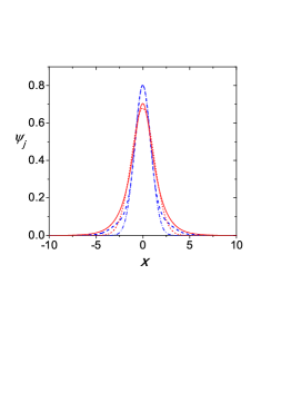
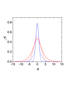
Figure 3: Profiles of BB solitons with $N_{1}=N_{2}=N$ corresponding to the $N=1$ points on the curves of Fig. 2 for attractive ($\gamma_{12}=-0.5$, left panel) and repulsive ($\gamma_{12}=0.1$, right panel) interspecies interaction. Blue (dashed and dot-dashed) and red (continuous and dotted) curves refer to first and second component, respectively. In both panels continuous and dashed lines refer to numerical solutions of Eqs. (4) found by relaxation method, while dotted and dot-dashed lines to variational analysis.

From Fig. 2 one can see that, while in the attractive case the agreement is quite good for a wide range of $N$ (this is true also for relatively large values of $\gamma_{12}$), in the repulsive case deviations of the VA and numerical curves are larger. This discrepancy is due to the fact that the Gaussian Ansatz becomes less accurate in the repulsive case, in which the interspecies interaction reduces the stability of the overlapped configuration, as one can see from Fig. 3 where VA and GPE solitons profiles are compared. However, the accuracy of the VA result increases as positive $\gamma_{12}$ values are decreased towards the uncoupling limit $\gamma_{12}=0$. Also note the existence of points where the chemical potential curves intersect, both for attractive and repulsive interspecies interactions. At these points, BB solitons, having the same number of atoms and the same chemical potentials (related to their width), will have equal VA profiles for the two components. Despite the discrepancy in the location of the intersection point, equality of profiles is well confirmed by numerical GPE results.

III Split BB solitons and dynamical properties

In the previous section, the choice of Gaussian trial wave functions (9) aimed at studying overlapped BB soliton configurations, with the peaks of the two density profiles coinciding at $x=0$. Due to attractive interspecies interaction, this configuration is expected to be the lowest-energy BB soliton pair. It is possible however to extend the analysis to split BB solitons, in which the centers of mass of the two species do not coincide.

Let us initially consider the uncoupled limit $\gamma_{12}=0$. In the case $V_{01}<0$ and $V_{02}<0$, one expects an infinite set of degenerate energy-minimizing BB solitons, since the centers of mass of each species can be located at any point $x_{0j}$ such that $\cos(2x_{0j})=0$, regardless of the other species’ density profile. These minimizing configurations can be classified in families

$$BB_{n}(\gamma_{12}=0),\qquad\textrm{with}\;n\in\mathbb{N},$$ (14)

according to the absolute distance between the centers of mass:

$$\Delta x:=|x_{02}-x_{01}|\in\left(\!\left(n-\frac{1}{2}\right)\!\pi,\!\left(n+\frac{1}{2}\right)\!\pi\right).$$ (15)

Clearly, the energy of the BB soliton configurations is the same for all families, $E_{n}(\gamma_{12}=0)=E_{0}$. When the effect of the interspecies coupling $\gamma_{12}$ can be treated as a small perturbation, one expects the existence of stationary Gross-Pitaevskii solutions close to the ones at $\gamma_{12}=0$, which can still be classified in families $BB_{n}(\gamma_{12})$ according to the criterion (15). However, if $\gamma_{12}<0$, the interspecies attraction will break the energetic degeneracy in favor of the overlapped configuration $BB_{0}$. Thus, the split solitons in $BB_{n>0}(\gamma_{12})$ become metastable. While configurations with a very large distance between the two species are almost unaffected by interspecies interactions, larger values of $|\gamma_{12}|$ weaken the (local) stability of solitons with small $n$, since attractive interactions can give a sufficient amount of energy to overcome the (linear or nonlinear) potential barrier and reduce the distance between the centers of mass. Thus, one expects a critical value $\gamma_{\mathrm{cr}}^{(n)}$, such that for $\gamma_{12}<\gamma_{\mathrm{cr}}^{(n)}$ metastable solutions in $BB_{n}$ would no longer exist.

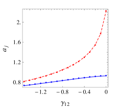
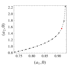
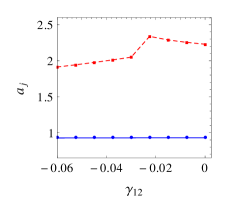
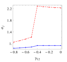
Figure 4: Numerical minimization of the pseudopotential $\Pi$ [see (22)-(23a) with soliton peaks around $(x_{01},x_{02})=(0,0)$ (top line), $(x_{01},x_{02})=(\pi,0)$ (central line), $(x_{01},x_{02})=(\pi,-\pi)$ (bottom line). Plots in the left column represent the variation of the optimal soliton widths $a_{1}$ (solid blue lines) and $a_{2}$ (dashed red lines) with $\gamma_{12}$. Plots in the right column show the behavior of one optimal width with respect to the other. The jumps observed in the central and bottom lines (right column) are due to the disappearance of local minima with $\Delta x\simeq\pi$ and $\Delta x\simeq 2\pi$ as $\gamma_{12}$ decreases under a critical value. Minima found below the critical $\gamma_{12}$ coincide with the values in the top plots and are thus not shown in the right column.

$\gamma_{12}$	$n$	$\quad\Delta x\quad$	$\quad a_{1}\quad$	$\quad a_{2}\quad$	$\quad\Pi_{\min}\quad$
0	0,1,2	$0,\pi,2\pi$	$0.929$	$2.229$	$-0.177$
$-0.25$	0	0	$0.910$	$1.472$	$-0.249$
$-0.25$	1	no local minimum
$-0.25$	2	$2.991\,\pi$	$0.930$	$2.260$	$-0.177$

Table 1: Locally stable BB soliton pairs for $N_{1}=1$, $N_{2}=1$, $\gamma_{1}=-1$, $\gamma_{2}=-1$, $V_{01}=-0.5$, $V_{02}=-0.25$, belonging to the classes $BB_{n}$ with $n=0,1,2$. The optimal parameters $\Delta x$, $a_{1}$ and $a_{2}$ (units of $k_{L}^{-1}$) are obtained by minimizing the global potential $\Pi$ (units of $2E_{r}$).

In the following, we will numerically analyze the existence of split BB soliton pairs, as well as their energetic and dynamical behavior. To this end, we shall generalize our Ansatz to include the positions of the component density centers as free parameters. We will also consider time-dependent parameters to investigate the dynamics of the system. The Gross-Pitaevskii equations (4) can be restated as a variational problem anderson

$$\delta\int{\cal{L}}\left(\psi_{j},\psi^{*}_{j},\frac{\partial\psi_{j}}{\partial x},\frac{\partial\psi^{*}_{j}}{\partial x},\frac{\partial\psi_{j}}{\partial t},\frac{\partial\psi^{*}_{j}}{\partial t}\right)\!\mathrm{d}x\,\mathrm{d}t=0,$$ (16)

where the Lagrangian density reads

$${\mathcal{L}} = \frac{1}{2}\sum_{j=1}^{2}\left[i\!\left(\psi^{*}_{j}\frac{\partial\psi_{j}}{\partial t}-\psi_{j}\frac{\partial\psi^{*}_{j}}{\partial t}\right)\!-\!\left|\frac{\partial\psi_{j}}{\partial x}\right|^{2}-\gamma_{j}|\psi_{j}|^{4}\right]$$ (17)

$$-V_{01}\cos(2x)|\psi_{1}|^{2}-\frac{V_{02}}{2}\cos(2x)|\psi_{2}|^{4}$$

$$-\gamma_{12}|\psi_{1}|^{2}|\psi_{2}|^{2}.$$

We generalize the Gaussian Ansatz (9) to

$$\psi_{j}(x,t) = A_{j}\exp\left[\mathrm{i}\frac{\mathrm{d}{x}_{0j}}{\mathrm{d}t}(x-x_{0j})+\mathrm{i}\phi_{j}(x-x_{0j})^{2}+\mathrm{i}\theta_{j}\right]$$ (18)

$$\times\exp\left[-\frac{(x-x_{0j})^{2}}{2a_{j}^{2}}\right],$$

where the variational parameters $(A_{j},a_{j},x_{0j},\phi_{j},\theta_{j})$ for $j=1,2$ are generally time-dependent and represent, respectively, the amplitude, width, center-of-mass position, frequency chirp and overall phase of a soliton in the $j$-th component. The Lagrangian $L$ for the trial wave functions (18), obtained by integrating the Lagrangian density in (17), reads

$$L = \int_{-\infty}^{+\infty}\,\,{\cal L}\,\,\mathrm{d}x$$ (19)

$$= \frac{\sqrt{\pi}}{4}\left(\sum_{j=1}^{2}\left[\frac{A_{j}^{2}}{a_{j}}+\sqrt{2}\gamma_{j}a_{j}A_{j}^{4}+4a_{j}^{3}A_{j}^{2}\phi_{j}^{2}\right.\right.$$

$$-\left.\left.2a_{j}A_{j}^{2}\left(\frac{\mathrm{d}x_{0j}}{\mathrm{d}t}\right)^{2}+4a_{j}A_{j}^{2}\frac{{\mathrm{d}\theta}_{j}}{\mathrm{d}t}+2a_{j}^{3}A_{j}^{2}\frac{\mathrm{d}\phi_{j}}{\mathrm{d}t}\right]\right.$$

$$+\left.4V_{01}\mathrm{e}^{-a_{1}^{2}}a_{1}A_{1}^{2}\cos(2x_{01})\right.$$

$$+\left.\sqrt{2}V_{02}\mathrm{e}^{-\frac{1}{2}a_{2}^{2}}a_{2}A_{2}^{4}\cos(2x_{02})\right.$$

$$+\left.\frac{4\gamma_{12}\,\mathrm{e}^{-\frac{(x_{01}-x_{02})^{2}}{{a_{1}}^{2}+{a_{2}}^{2}}}a_{1}A_{1}^{2}a_{2}A_{2}^{2}}{\sqrt{{a_{1}}^{2}+{a_{2}}^{2}}}\right).$$

Note the dependence of the interaction term on $\Delta x$, defined in (15).

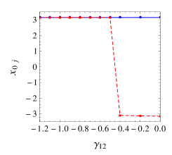
Figure 5: Left panel. Peak positions $x_{01}$ (solid blue line) and $(x_{02})$ (dotted red line) of optimal BB profiles, obtained by searching the local minimum around $(x_{01},x_{02})=(\pi,-\pi)$, for different values of $\gamma_{12}$. The sudden jump towards $(\pi,\pi)$ is due to the disappearance of the local minimum (see also Fig. 4, bottom panels). Right panel. Local minimum value of the effective potential energy in Eq. (22).

The functional derivatives of $L$ with respect to the variational parameters yield a set of Euler-Lagrange equations. After appropriate manipulation, we can obtain a picture for the dynamics of the soliton pairs. In particular, the equations

$$\frac{\mathrm{d}}{\mathrm{d}t}(\sqrt{\pi}a_{j}A_{j}^{2}) = 0,$$ (20)

$$-2a_{j}\phi_{j}+\frac{\mathrm{d}{a}_{j}}{\mathrm{d}t} = 0$$ (21)

can be interpreted as dynamical constraints on the amplitude (particle numbers conservation) and the frequency chirp. Taking into account (20)-(21), the equations of motion for the centers of mass and the width can all be derived from the effective potential

$$\Pi\left(a_{1},a_{2},x_{01},x_{02}\right) = \Pi_{1}\left(a_{1},x_{01}\right)+\Pi_{2}\left(a_{2},x_{02}\right)$$ (22)

$$+ \Pi_{12}\left(a_{1},x_{01},a_{2},x_{02}\right),$$

with

$$\Pi_{1}\left(a_{1},x_{01}\right) = \frac{N_{1}}{4a_{1}^{2}}+\frac{\gamma_{1}N_{1}^{2}}{2\sqrt{2\pi}a_{1}}$$ (23a)

$$+\mathrm{e}^{-{a_{1}}^{2}}N_{1}V_{01}\cos(2x_{01}),$$

$$\Pi_{2}\left(a_{2},x_{02}\right) = \frac{N_{2}}{4a_{2}^{2}}+\frac{\gamma_{2}N_{2}^{2}}{2\sqrt{2\pi}a_{2}}$$ (23b)

$$+\frac{\mathrm{e}^{-\frac{1}{2}{a_{2}}^{2}}N_{2}^{2}V_{02}\cos(2x_{02})}{2\sqrt{2\pi}{a_{2}}},$$

$$\Pi_{12}\left(a_{1},x_{01},a_{2},x_{02}\right)=\frac{\mathrm{e}^{-\frac{(x_{01}-x_{02})^{2}}{{a_{1}}^{2}+{a_{2}}^{2}}}\gamma_{12}N_{1}N_{2}}{\sqrt{\pi}\sqrt{{a_{1}}^{2}+{a_{2}}^{2}}},$$ (23c)

through the Newton-like equations

$$\frac{\mathrm{d}^{2}}{\mathrm{d}t^{2}}\begin{pmatrix}N_{1}x_{01}\\ N_{2}x_{02}\\ (N_{1}/2)a_{1}\\ (N_{2}/2)a_{2}\end{pmatrix}=-\begin{pmatrix}\partial_{x_{01}}\\ \partial_{x_{02}}\\ \partial_{a_{1}}\\ \partial_{a_{2}}\end{pmatrix}\Pi\left(a_{1},a_{2},x_{01},x_{02}\right).$$ (24)

The problem of finding stationary solutions within the Ansatz (18) thus reduces to searching the minima of the effective potential. The equations (24) can also be linearized around the stable equilibrium points for $\Pi$, to obtain information on small center-of-mass and width oscillations. On the other hand, due to the (still restrictive) form of the trial wave functions, the far-from-equilibrium dynamics of Eqs. (24) cannot be considered physically relevant (see the discussion below.) In Table 1, we show some illustrative results of the optimal parameters $\Delta x$, $a_{1}$ and $a_{2}$ for solitons in the classes $BB_{n}$ with $n=0,1,2$. The numbers of particles are fixed to $N_{1}=N_{2}=1$. At $\gamma_{12}=0$, the three minima are degenerate. At $\gamma_{12}=-0.25$, the split solitons in the family $BB_{2}$ are locally stable [see Eq. (14)], while the global minimum is, as expected, the overlapped configuration. Instead, no local minimum can be found in the family $BB_{1}$, indicating that $\gamma_{\mathrm{cr}}^{(1)}>-0.25$.

A more systematic picture of the existence and behavior of solitons for small $n$ with varying $\gamma_{12}$ is given in Fig. 4: a numerical minimization procedure is used to find stable configurations with their centers of mass close to some initial points $(\tilde{x}_{01},\tilde{x}_{02})$. A minimum with centers of mass around $(\tilde{x}_{01},\tilde{x}_{02})=(0,0)$ can be found for all negative $\gamma_{12}$ (top panels). On the other hand, the search of minima whose centers of mass are close to $(\tilde{x}_{01},\tilde{x}_{02})=(\pi,0)$ and $(\tilde{x}_{01},\tilde{x}_{02})=(-\pi,\pi)$ yields discontinuous behaviors in the optimal parameters (central and bottom panels). The discontinuities are present because solitons in $BB_{1}$ (respectively $BB_{2}$) exist only for $\gamma_{12}>\gamma_{\mathrm{cr}}^{(1)}$ (respectively $\gamma_{12}>\gamma_{\mathrm{cr}}^{(2)}$), while for more negative values the algorithm actually finds the global minimum belonging to $BB_{0}$. It is also worth noticing that in Fig. 4 the optimal widths $a_{1}$ and $a_{2}$ of the overlapped solitons decrease with $|\gamma_{12}|$. In the case of split solitons, the amplitudes remain almost constant, with a slight increase (more evident in $a_{2}$) with $|\gamma_{12}|$, due to the attraction exerted between densities.

These findings are corroborated by the behavior of the center-of-mass positions displayed in Fig. 5, where the displacement of the center of mass of the second species with increasing interspecies interaction is observed. The situation is the same as that depicted in Fig. 4, bottom panels. In the left panel of Fig. 5, the jump of $x_{02}$ as $|\gamma_{12}|$ is decreased signals the disappearance of the local energy minimum. The value of the local minimum of the effective potential energy (22) is shown in the right panel.

 

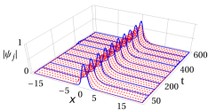
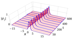
Figure 6: Time evolution of density profiles for overlapped solitons in the first (blue solid lines) and second (red dashed lines) species for $\gamma_{12}=-0.25$ (left panel) and $\gamma_{12}=-1$ (right panel). The results are obtained by direct numerical integration.

 

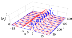
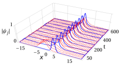
Figure 7: Time evolution of density profiles for split solitons in the first (blue solid lines) and second (red dashed lines) species for $\gamma_{12}=-0.25$ (left panel) and $\gamma_{12}=-0.38$ (right panel). In the latter case, numerical integration shows the instability of the soliton pair.

In order to check the existence and stability of BB soliton pairs as approximate solutions of the GPEs, we employ a numerical simulation of the dynamics generated by (4). First, we have checked the stationarity of overlapped soliton pairs, localized around $x=0$. It is possible to verify, for different values of $\gamma_{12}$, that the soliton pair determined by the minimization procedure is stationary within very good approximation. In Fig. 6, the time evolution of the overlapped solitons is represented for $\gamma_{12}=-0.25$ (left) and $\gamma_{12}=-1$ (right). Then, we have tested the behavior of split soliton pairs in $BB_{2}$ in different regimes. In the case $\gamma_{12}=-0.25$, which is larger than the critical value $\gamma_{\mathrm{cr}}^{(2)}\simeq-0.4$, the split configuration evolves in time with slight distortions, but it preserves the qualitative features of the initial state for all the time of the simulation (left panel of Fig. 7). When $\gamma_{12}\simeq\gamma_{\mathrm{cr}}^{(2)}$, the energetic instability of the soliton pair in $BB_{2}$ is reflected by a dynamical instability: the second-species density distribution is gradually attracted by the first species (right panel of Fig. 7), ending with an overlapped configuration, which is eventually stabilized by radiating wave packets Yulin ; garnier .

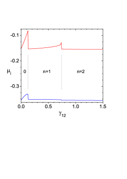
Figure 8: Dependence of chemical potentials (left panel) and distance between peaks (right panel) on repulsive interspecies interactions of a BB soliton with $N_{1}=N_{2}=1$. Other parameters are fixed as $\gamma_{1}=\gamma_{2}=-1,V_{01}=-0.5,V_{02}=-0.25$. Top (blue) and bottom (red) curves in the left panel refer to chemical potentials of first and second component, respectively, while vertical lines separate $\gamma_{12}$ regions for existence of BB solitons in $BB_{0}$ (overlapped), $BB_{1}$ and $BB_{2}$ (split).

IV Splitting dependence on interspecies interaction

In the previous section we observed that split BB solitons can become unstable at some negative critical values of the interspecies scattering length. We shall now investigate these critical values in more detail by direct numerical integration of the GPEs, both for attractive and repulsive interatomic interactions.

Let us first discuss the repulsive case. We can consider as initial state an overlapped BB soliton, centered at $x=0$, with no interspecies coupling $(\gamma_{12}=0)$, and adiabatically switch on a repulsive interspecies interaction between components at $t>0$. One expects that, due to the repulsive interspecies interaction, the initial $BB_{0}$ soliton will evolve into a split one belonging to the $BB_{1}$ family at some value $\gamma_{12}=\gamma_{\mathrm{rep}}^{(1)}$ and then into the $BB_{2}$ family at $\gamma_{12}=\gamma_{\mathrm{rep}}^{(2)}$. This picture coincides with the numerical results in Fig. 8, both in terms of the chemical potentials and the distances between peaks $\Delta x$, normalized to $\pi$. The jumps in the distance are correlated with jumps in the chemical potentials at the critical values, which are uniquely fixed by the parameters of the system. In Fig. 9, the profiles of the split solitons with $n=1$ and $n=2$ are represented, at two different $\gamma_{12}$ values belonging to their existence curve. Despite the smaller value of $\gamma_{12}$, the two BB components in the $n=1$ case appear to be more distorted in their overlapping region than in the $n=2$ case. This is an evident consequence of the exponential decay of the soliton-soliton interaction with distance [see Eq. (19)]. Notice that, as in the attractive case, the normalized distance between soliton centers is not an integer number. This is a clear consequence of the existence of a repulsive force between components.

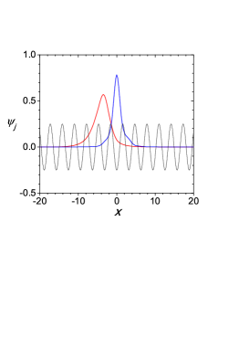
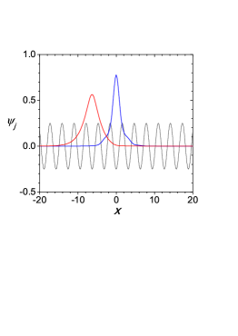
Figure 9: Split BB solitons inside the regions $n=1$ and $n=2$ of the left panel of Fig. 8, at $\gamma_{12}=0.5$ (left panel) and $\gamma_{12}=1.0$ (right panel). The blue (curve centered at zero) and red profiles refer to first and second component, respectively, while the black line shows the periodicity of the optical lattice.

When attractive interactions $\gamma_{12}<0$ are adiabatically turned on at $t>0$, we expect that an initial split soliton in $BB_{n_{0}}$, with $n_{0}>0$, will undergo only one jump towards $n=0$. Indeed, from the analysis in the previous section, we can deduce that the negative critical values are ordered as $\gamma_{\mathrm{cr}}^{(n)}>\gamma_{\mathrm{cr}}^{(n+1)}$. Thus, if $\gamma_{12}>\gamma_{\mathrm{cr}}^{(n_{0})}$, interactions give enough energy to overcome all the intermediate barriers from the $n_{0}$-th down to $n=0$. This intuitive result, based on energetic considerations, match very well the results of the numerical simulation, as one can see from Fig. 10, where the cases $n_{0}=2$ and $n_{0}=1$ are represented.

Since the critical values of $\gamma_{12}$ at which the transitions occur are uniquely fixed by the parameters of the mixture, including the number of atoms and intraspecies interactions, an experimental implementation of the above numerical simulations could be used for indirect measurements of the interspecies scattering length of BEC mixtures. The interspecies scattering length can also be measured from the oscillatory motion of coupled solitons as predicted in sekh .

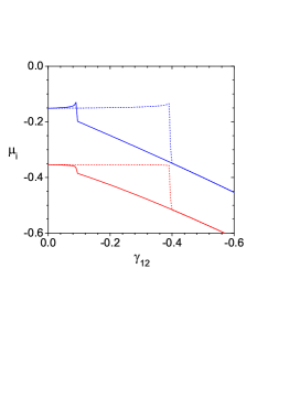
Figure 10: Dependence on attractive interspecies interaction of chemical potentials (left panel) and distance between density centers, $x_{1},x_{2}$, (right panel) of a BB soliton with $N_{1}=N_{2}=1$. Bottom (blue) and top (red) curves in the left panel refer to the first and the second component, respectively, while dotted and continuous lines (left panel) and square and triangle symbols (right panel) refer to BB solitons with centers initially separated by $\pi$ and by $2\pi$, respectively. Other parameters are fixed as $\gamma_{1}=\gamma_{2}=-1,V_{01}=-0.5,V_{02}=-0.25$.

V Conclusions

We have considered matter-wave bright-bright solitons in coupled Bose-Einstein condensates, by assuming that the first component is loaded in a linear optical lattice and the second component in a nonlinear optical lattice. In particular, the existence and stability of split and overlapped BB solitons has been investigated by VA, by direct numerical integrations of the coupled GPEs, and by direct numerical integrations of the system. The dependence of the existence ranges of BB solitons on the interspecies interaction parameter has been also investigated. In particular, for repulsive interspecies interactions we showed the existence of a series of critical values of $\gamma_{12}$ at which transitions from the $n$- to the $n+1$- split BB soliton occur. For attractive interspecies interaction we showed that only direct transitions from a split BB solitons to the overlapped BB soliton are possible. Since critical values at which transitions occur depend on physical parameters of the mixture, these phenomena suggest that split BB solitons could be used for indirect measurements of these parameters in experiments.

References

- (1) I. Bloch, J. Dalibard, W. Zwerger, Rev. Mod. Phys. 80, 885 (2008).
- (2) M. Theis, G. Thalhammer, K. Winkler, M. Hellwig, G. Ruff, R. Grimm, J.H. Denschlag, Phys. Rev. Lett. 93, 123001 (2004).
- (3) O. Morsch, J. H. Muller, M. Cristiani, D. Ciampini, and E. Arimondo, Phys. Rev. Lett. 87, 140402 (2001).
- (4) M. Salerno, V.V. Konotop, Y.V. Bludov, Phys. Rev. Lett. 101, 030405 (2008).
- (5) B. P. Anderson and M. A. Kasevich, Science 282, 1686 (1998).
- (6) H. Lignier, C. Sias, D. Ciampini, Y. Singh, A. Zenesini, O. Morsch, and E. Arimondo, Phys. Rev. Lett. 99, 220403 (2007).
- (7) A. Zenesini, H. Lignier, D. Ciampini, O. Morsch, and E. Arimondo, Phys. Rev. Lett. 102, 100403 (2009).
- (8) M. Jona-Lasinio, O. Morsch, M. Cristiani, N. Malossi, J. H. M ller, E. Courtade, M. Anderlini, and E. Arimondo, Phys. Rev. Lett. 91, 230406 (2003).
- (9) S. Wimberger, R. Mannella, O. Morsch, E. Arimondo, A. Kolovsky, A. Buchleitner, Phys. Rev. A 72, 063610 (2005).
- (10) A. Zenesini, H. Lignier, G. Tayebirad, J. Radogostowicz, D. Ciampini, R. Mannella, S. Wimberger, O. Morsch, and E. Arimondo, Phys. Rev. Lett. 103, 090403 (2009).
- (11) M. Greiner, O. Mandel, T. Esslinger, T.W. Hänsch and I. Bloch, Nature (London) 415, 39 (2002).
- (12) V.V. Konotop, M. Salerno, Phys. Rev. A 65, (2002) 021602.
- (13) G.L. Alfimov, V.V. Konotop, and M. Salerno, Europhys. Lett. 58, 7 (2002).
- (14) I. Carusotto, D. Embriaco, and G. C. La Rocca, Phys. Rev. A 65, 053611 (2002).
- (15) M. Salerno, Laser Phys. 15, 620 (2005).
- (16) G. A. Sekh, Phys. Lett. A 376, 1740 (2012).
- (17) G. A. Sekh, Pramana: J. Phys. 81 , 261 (2013).
- (18) B.B. Baizakov, V.V. Konotop, and M. Salerno, J. Phys. B 35, 5105 (2002).
- (19) B.B. Baizakov, B.A. Malomed, and Mario Salerno, Europhys. Lett. 63, 642 (2003); Phys. Rev. A. 70, 053613 (2004).
- (20) F. Kh. Abdullaev and M. Salerno, Phys. Rev. A 72, 033617 (2005).
- (21) A. Trombettoni and A. Smerzi, Phys. Rev. Lett. 86, 2353 (2001).
- (22) F.Kh. Abdullaev, B.B. Baizakov, S.A. Darmanyan, V.V. Konotop, and M. Salerno, Phys. Rev. A 64 , 043606 (2001).
- (23) Y. V. Kartashov, B. A. Malomed, and L. Torner, Rev. Mod. Phys. 83, 405 (2011).
- (24) F.Kh. Abdullaev, A. Gammal, M. Salerno, and Lauro Tomio, Phys. Rev. A 82, 043618 (2010).
- (25) F.Kh. Abdullaev, A. Gammal, H.L.F. da Luz, M. Salerno, and Lauro Tomio, J. Phys. B: At. Mol. Opt. Phys. 45, 115302 (2012).
- (26) Y. Bludov, V.V. Konotop, and M. Salerno, J. Phys. B: At. Mol. Opt. Phys. 42, 105302 (2009).
- (27) Yu. V. Bludov, V. V. Konotop, and M. Salerno, Phys. Rev. A 80, 023623 (2009); Phys. Rev. A 81, 053614 (2010).
- (28) Yu. V. Bludov, V. V. Konotop, and M. Salerno, Europhys. Lett. 87, 20004 (2009).
- (29) V. A. Brazhnyi and V. V. Konotop, Mod. Phys. Lett. B 18, 627 (2004).
- (30) O. Morsch and M. Oberthaler, Rev. Mod. Phys. 78, 179 (2006).
- (31) I. Bloch, J. Dalibard, and W. Zwerger, Rev. Mod. Phys. 80, 885 (2008).
- (32) N.A. Kostov, V.Z. Enolskii, V.S. Gerdjikov, V.V. Konotop, and M. Salerno, Phys. Rev. E 70, 056617 (2004).
- (33) H.A. Cruz, V.A. Brazhnyi, V.V. Konotop, G.L. Alfimov, and M. Salerno, Phys. Rev. A 76, 013603 (2007).
- (34) P. Facchi, G. Florio, S. Pascazio, and F. V. Pepe, J. Phys. A: Math. Theor. 44, 505305 (2011).
- (35) F. V. Pepe, P. Facchi, G. Florio, and S. Pascazio, Phys. Rev. A 86, 023629 (2012).
- (36) V. A. Brazhnyi, D. Novoa, and C. P. Jisha, Phys. Rev. A 88, 013629 (2013).
- (37) B. Van Schaeybroeck and J. O. Indekeu, Phys. Rev. A 91, 013626 (2015).
- (38) A. I. Yakimenko, K. O. Shchebetovska, S. I. Vilchinskii, and M. Weyrauch, Phys. Rev. A 85, 053640 (2012).
- (39) S. K. Adhikari and B. A. Malomed, Phys. Rev. A 77, 023607(2008)
- (40) F. Kh. Abdullaev, A. Gammal, M. Salerno, L. Tomio, Phys. Rev. A. 77, 023615 (2008)
- (41) Sk. Golam Ali and B. Talukdar, Ann. Phys. 324, 1194 (2009).
- (42) Y. Cheng, J. Phys. B: At. Mol. Opt. Phys. 42, 205005 (2009).
- (43) I. Vidanovic, A. Balaz, H. Al-Jibbouri, A. Pelster, Phys. Rev. A 84, 013618 (2011).
- (44) A. Balaz, I. Vidanovic, A. Bogojevic, and A. Pelster, Phys. Lett. A 374, 1539 (2010).
- (45) L. Pitaevskii and S. Stringari, Bose-Einstein Condensation (Oxford University Press, Oxford, 2003).
- (46) M. G. Vakhitov, A. A. Kolokolov, Izv. Vyssh. Uch. Zav. Radiofizika 16, 1020 (1973) [English Transl. Radiophys. Quant. Electron. 39, 51].
- (47) L. Khaykovich, F. Schreck, G. Ferrari, T. Bourdel, J. Cubizolles, L. D. Carr, Y. Castin and C. Salomon, Science 296, 1290 (2002).
- (48) A. L. Marchant, , T. P. Billam, T. P. Wiles, M. M. H. Yu, S. A. Gardiner, and S. L. Cornish, Nature Communications 4, 1865, (2013).
- (49) D. Anderson, Phys. Rev. A 27, 3135 (1983).
- (50) A. V. Yulin, D. V. Skryabin, and P. St. J. Russell, Phys. Rev. Lett. 91, 260402 (2003).
- (51) F. Kh. Abdullaev and J. Garnier, Phys. Rev. A 72, 061605(R) (2005).
- (52) G. A. Sekh and M. Salerno, A. Saha and B. Talukdar, Phys. Rev. A 85, 023639 (2012).