Instantly Decodable Network Coding for Real-Time Scalable Video Broadcast over Wireless Networks

Abstract

In this paper, we study a real-time scalable video broadcast over wireless networks in instantly decodable network coded (IDNC) systems. Such real-time scalable video has a hard deadline and imposes a decoding order on the video layers. We first derive the upper bound on the probability that the individual completion times of all receivers meet the deadline. Using this probability, we design two prioritized IDNC algorithms, namely the expanding window IDNC (EW-IDNC) algorithm and the non-overlapping window IDNC (NOW-IDNC) algorithm. These algorithms provide a high level of protection to the most important video layer before considering additional video layers in coding decisions. Moreover, in these algorithms, we select an appropriate packet combination over a given number of video layers so that these video layers are decoded by the maximum number of receivers before the deadline. We formulate this packet selection problem as a two-stage maximal clique selection problem over an IDNC graph. Simulation results over a real scalable video stream show that our proposed EW-IDNC and NOW-IDNC algorithms improve the received video quality compared to the existing IDNC algorithms.

I Introduction

Network coding has shown great potential to improve throughput, delay and quality of services in wireless networks [1, 2, 3, 4, 5, 6, 7, 8, 9, 10, 11, 12, 13]. These merits of network coding make it an attractive candidate for multimedia applications [10, 11, 12]. In this paper, we are interested in real-time scalable video applications [14, 15], which compress video frames in the form of one base layer and several enhancement layers. The base layer provides the basic video quality and the enhancement layers provide successive improved video qualities. Using such a scalable video stream, the sender adapts a video bit rate to the available network bandwidth by sending the base layer and as many enhancement layers as possible. Moreover, the real-time scalable video has two distinct characteristics. First, it has a hard deadline such that the video layers need to be decoded on-time to be usable at the applications. Second, the video layers exhibit a hierarchical order such that a video layer can be decoded only if this layer and all its lower layers are received. Even though scalable video can tolerate the loss of one or more enhancement layers, this adversely affects the video quality experienced by viewers. Therefore, it is desirable to design network coding schemes so that the received packets before the deadline contribute to decoding the maximum number of video layers.

Network coding schemes are often adopted and designed to be suitable for different applications. For example, the works in [16, 17, 18, 19] adopted random linear network coding (RLNC) strategies for scalable video transmission and designed window based RLNC such that coded packets are formed across all packets in different numbers of video layers. In particular, the authors in [16] used a probabilistic approach for selecting coding windows and included the packets in the lower video layers into all coded packets to obtain high decoding probabilities for the lower layers. However, the authors in [18] considered a scalable video transmission with a hard deadline and used a deterministic approach for selecting coding windows over all transmissions before the deadline. Despite the best throughput performance of RLNC, in this paper, we adopt instantly decodable network coding (IDNC) strategies due to its several attractive properties [8, 9, 20, 21, 22, 23, 24, 25, 26]. IDNC aims to provide instant packet decodability upon successful packet reception at the receivers. This instant decodability property allows a progressive recovery of the video layers as the receivers decode more packets. Furthermore, the encoding process of IDNC is performed using simple XOR operations compared to more complicated operations over large Galois fields performed in RLNC. The XOR operations also reduce packet overhead compared to the coefficient reporting overhead required in RLNC. The decoding process of IDNC is performed using XOR operations, which is suitable for implementation in simple and cost-efficient receivers, compared to complex matrix inversion performed in RLNC.

Due to these attractive properties, the authors in [20, 21, 22, 23] considered IDNC for wireless broadcast of a set of packets and aimed to service the maximum number of receivers with a new packet in each transmission. In [24, 25], the authors addressed the problem of minimizing the number of transmissions required for broadcasting a set of packets in IDNC systems and formulated the problem into a stochastic shortest path (SSP) framework. However, the works in [20, 21, 22, 23, 24, 25] neither considered dependency between source packets to use at the applications nor considered explicit packet delivery deadline. Several other works in IDNC considered different importance of packets and prioritized packets differently in coding decisions. In particular, the authors in [8] adopted IDNC for video streaming and showed that their proposed IDNC schemes are asymptotically throughput optimal for the three-receivers system subject to sequential packet delivery deadline constraints. However, the work in [8] neither considered dependency between source packets as is present in the scalable video applications nor considered an arbitrary number of receivers. Another work in [11] considered a single layer video transmission and determined the importance of each video packet based on its contribution to the video quality. The selected IDNC packet in [11] maximized the video quality in the current transmission without taking into account the coding opportunities and the video quality over the successor transmissions before the deadline.

In the context of IDNC for scalable video with multiple layers, the most related works to ours are [27, 28]. In [27], the authors considered that a set of packets forming the base layer has high priority compared to an another set of packets forming the enhancement layers. However, the IDNC algorithms in [27] aimed to reduce the number of transmissions required for delivering all the packets instead of giving priority to reducing the number of transmissions required for delivering the high priority packets. The coding decisions in [27] also searched for the existence of a special IDNC packet that can simultaneously reduce the number of transmissions required for delivering the high priority packets and the number of transmissions required for delivering all the packets. On the other hand, the authors in [28] discussed the hierarchical order of video layers with motivating examples and proposed a heuristic packet selection algorithm. The IDNC algorithm in [28] aimed to balance between the number of transmissions required for delivering the base layer and the number of transmissions required for delivering all video layers. Both works in [27, 28] ignored the hard deadline and did not strictly prioritize to deliver the base layer packets before the deadline. However, for real-time scalable video transmission, addressing the hard deadline for the base layer packets is essential as all other packets depend on the base layer packets.

In this paper, inspired by real-time scalable video that has a hard deadline and decoding dependency between video layers, we are interested in designing an efficient IDNC framework that maximizes the minimum number of decoded video layers over all receivers before the deadline (i.e., improves fairness in terms of the minimum video quality across all receivers). In such scenarios, by taking into account the deadline, IDNC schemes need to make coding decisions over the packets in the first video layer or the packets in all video layers. While the former guarantees the highest level of protection to the first video layer, the latter increases the possibility of decoding a large number of video layers before the deadline. In this context, our main contributions are summarized as follows.

• We derive the upper bound on the probability that the individual completion times of all receivers for a given number of video layers meet the deadline. Using this probability, we are able to approximately determine whether the broadcast of any given number of video layers can be completed before the deadline with a predefined probability.

• We design two prioritized IDNC algorithms for scalable video, namely the expanding window IDNC (EW-IDNC) algorithm and the non-overlapping window IDNC (NOW-IDNC) algorithm. EW-IDNC algorithm selects a packet combination over the first video layer and computes the resulting upper bound on the probability that the broadcast of that video layer can be completed before the deadline. Only when this probability meets a predefined high threshold, the algorithm considers additional video layers in coding decisions in order to increase the number of decoded video layers at the receivers.

• In EW-IDNC and NOW-IDNC algorithms, we select an appropriate packet combination over a given number of video layers that increases the possibility of decoding those video layers by the maximum number of receivers before the deadline. We formulate this problem as a two-stage maximal clique selection problem over an IDNC graph. However, the formulated maximal clique selection problem is NP-hard and even hard to approximate. Therefore, we exploit the properties of the problem formulation and design a computationally simple heuristic packet selection algorithm.

• We use a real scalable video stream to evaluate the performance of our proposed algorithms. Simulation results show that our proposed EW-IDNC and NOW-IDNC algorithms increase the minimum number of decoded video layers over all receivers compared to the IDNC algorithms in [23, 28] and achieve a similar performance compared to the expanding window RLNC algorithm in [16, 18] while preserving the benefits of IDNC strategies.

The rest of this paper is organized as follows. The system model and IDNC graph are described in Section II. We illustrate the importance of appropriately choosing a coding window in Section III and draw several guidelines for prioritized IDNC algorithms in Section IV. Using these guidelines, we design two prioritized IDNC algorithms in Section V. We formulate the problem of finding an appropriate packet combination in Section VI and design a heuristic packet selection algorithm in Section VII. Simulation results are presented in Section VIII. Finally, Section IX concludes the paper.

II Scalable Video Broadcast System

II-A Scalable Video Coding

We consider a system that employs the scalable video codec (SVC) extension to H.264/AVC video compression standard [14, 15]. A group of pictures (GOP) in scalable video has several video layers and the information bits of each video layer is divided into one or more packets. The video layers exhibit a hierarchical order such that each video layer can only be decoded after successfully receiving all the packets of this layer and its lower layers. The first video layer (known as the base layer) encodes the lowest temporal, spatial, and quality levels of the original video and the successor video layers (known as the enhancement layers) encode the difference between the video layers of higher temporal, spatial, and quality levels and the base layer. With the increase in the number of decoded video layers, the video quality improves at the receivers.

II-B System Model

We consider a wireless sender (e.g., a base station or a wireless access point) that wants to broadcast a set of $N$ source packets forming a GOP, $\mathcal{N}=\{P_{1},...,P_{N}\}$, to a set of $M$ receivers, $\mathcal{M}=\{R_{1},...,R_{M}\}$. A network coding scheme is applied on the packets of a single GOP as soon as all the packets are ready, which implies that neither merging of GOPs nor buffering of packets in more than one GOP at the sender is allowed. This significant aspect arises from the minimum delivery delay requirement in real-time video streaming. Time is slotted and the sender can transmit one packet per time slot $t$. There is a limit on the total number of allowable time slots $\Theta$ used to broadcast the $N$ packets to the $M$ receivers, as the deadline for the current GOP expires after $\Theta$ time slots. Therefore, at any time slot $t\in[1,2,...,\Theta]$, the sender can compute the number of remaining transmissions for the current GOP as, $Q=\Theta-t+1$.

In the scalable video broadcast system, the sender has $L$ scalable video layers and each video layer consists of one or more packets. Let the set $\mathcal{N}=\{P_{1}^{1},P_{2}^{1},...,P_{n_{1}}^{1},...,P_{1}^{L},P_{2}^{L},...,P_{n_{L}}^{L}\}$ denote all the packets in the $L$ video layers, with $n_{\ell}$ being the number of packets in the $\ell$-th video layer. In fact, $N=\sum_{\ell=1}^{L}n_{\ell}$. Although the number of video layers in a GOP of a video stream is fixed, depending on the video content, $n_{\ell}$ and $N$ can have different values for different GOPs. We denote the set that contains all packets in the first $\ell$ video layers as $\mathcal{N}^{1:\ell}$ and the cardinality of $\mathcal{N}^{1:\ell}$ as $N^{1:\ell}$.

The receivers are assumed to be heterogeneous (i.e., the channels between the sender and the receivers are not necessarily identical) and each transmitted packet is subject to an independent Bernoulli erasure at receiver $R_{i}$ with probability $\epsilon_{i}$. Each receiver listens to all transmitted packets and feeds back to the sender a positive or negative acknowledgement (ACK or NAK) for each received or lost packet. After each transmission, the sender stores the reception status of all packets at all receivers in an $M\times N$ state feedback matrix (SFM) $\mathbf{F}=[f_{i,j}],$ $\;\forall R_{i}\in\mathcal{M},P_{j}\in\mathcal{N}$ such that:

$$f_{i,j}=\begin{cases}0&\text{if packet $P_{j}$ is received by receiver $R_{i}$},\\ 1&\text{if packet $P_{j}$ is missing at receiver $R_{i}$}.\end{cases}$$ (1)

Example 1

An example of SFM with $M=2$ receivers and $N=5$ packets is given as follows:

$$\mathbf{F}=\begin{pmatrix}1&0&1&1&1\\ 0&1&1&0&0\\ \end{pmatrix}.$$ (2)

In this example, we assume that packets $P_{1}$ and $P_{2}$ belong to the first (i.e., base) layer, packets $P_{3}$ and $P_{4}$ belong to the second layer and packet $P_{5}$ belongs to the third layer. Therefore, the set containing all packets in the first two video layers is $\mathcal{N}^{1:2}=\{P_{1},P_{2},P_{3},P_{4}\}$.

Definition 1

A window over the first $\ell$ video layers (denoted by $\omega_{\ell}$) includes all the packets in $\mathcal{N}^{1:\ell}=\{P_{1}^{1},P_{2}^{1},...,P_{n_{1}}^{1},...,P_{1}^{\ell},P_{2}^{\ell},...,P_{n_{\ell}}^{\ell}\}$.

There are $L$ windows for a GOP with $L$ video layers as shown in Fig. 1. The SFM corresponding to the window $\omega_{\ell}$ over the first $\ell$ video layers is an $M\times N^{1:\ell}$ matrix $\mathbf{F}^{1:\ell}$, which contains the first $N^{1:\ell}$ columns of SFM $\mathbf{F}$.

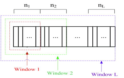
Figure 1: $L$ windows for an $L$-layer GOP with $n_{\ell}$ packets in the $\ell$-th layer.

Based on the SFM, the following two sets of packets can be attributed to each receiver $R_{i}$ at any given time slot $t$:

• The Has set of receiver $R_{i}$ in the first $\ell$ video layers ($\mathcal{H}_{i}^{1:\ell}$) is defined as the set of packets that are decoded by receiver $R_{i}$ from the first $\ell$ video layers. In Example 1, the Has set of receiver $R_{2}$ in the first two video layers is $\mathcal{H}_{2}^{1:2}=\{P_{1},P_{4}\}$.

• The Wants set of receiver $R_{i}$ in the first $\ell$ video layers ($\mathcal{W}_{i}^{1:\ell}$) is defined as the set of packets that are missing at receiver $R_{i}$ from the first $\ell$ video layers. In other words, $\mathcal{W}_{i}^{1:\ell}=\mathcal{N}^{1:\ell}\setminus\mathcal{H}_{i}^{1:\ell}$. In Example 1, the Wants set of receiver $R_{2}$ in the first two video layers is $\mathcal{W}_{2}^{1:2}=\{P_{2},P_{3}\}$.

The cardinalities of $\mathcal{H}_{i}^{1:\ell}$ and $\mathcal{W}_{i}^{1:\ell}$ are denoted by $H_{i}^{1:\ell}$ and $W_{i}^{1:\ell}$, respectively. The set of receivers having non-empty Wants sets in the first $\ell$ video layers is denoted by $\mathcal{M}_{w}^{1:\ell}$ (i.e., $\mathcal{M}_{w}^{1:\ell}=\left\{R_{i}\middle|\mathcal{W}_{i}^{1:\ell}\neq\varnothing\right\}$). At any given SFM $\mathbf{F}^{1:\ell}$ at time slot $t$, receiver $R_{i}$ having non-empty Wants set in the first $\ell$ video layers (i.e., $R_{i}\in\mathcal{M}_{w}^{1:\ell}$) belongs to one of the following three sets:

• The critical set of receivers for the first $\ell$ video layers ($\mathcal{C}^{1:\ell}$) is defined as the set of receivers with the number of missing packets in the first $\ell$ video layers being equal to the number of remaining $Q$ transmissions (i.e., $W_{i}^{1:\ell}=Q,\forall R_{i}\in\mathcal{C}^{1:\ell}$).

• The affected set of receivers for the first $\ell$ video layers ($\mathcal{A}^{1:\ell}$) is defined as the set of receivers with the number of missing packets in the first $\ell$ video layers being greater than the number of remaining $Q$ transmissions (i.e., $W_{i}^{1:\ell}>Q,\forall R_{i}\in\mathcal{A}^{1:\ell}$).

• The non-critical set of receivers for the first $\ell$ video layers ($\mathcal{B}^{1:\ell}$) is defined as the set of receivers with the number of missing packets in the first $\ell$ video layers being less than the number of remaining $Q$ transmissions (i.e., $W_{i}^{1:\ell}<Q,\forall R_{i}\in\mathcal{B}^{1:\ell}$).

In fact, $\mathcal{C}^{1:\ell}\cup\mathcal{A}^{1:\ell}\cup\mathcal{B}^{1:\ell}=\mathcal{M}_{w}^{1:\ell}$. We denote the cardinalities of $\mathcal{C}^{1:\ell}$, $\mathcal{A}^{1:\ell}$ and $\mathcal{B}^{1:\ell}$ as $C^{1:\ell}$, $A^{1:\ell}$ and $B^{1:\ell}$, respectively.

Definition 2

A transmitted packet is instantly decodable for receiver $R_{i}$ if it contains exactly one source packet from $\mathcal{W}_{i}^{1:L}$.

Definition 3

Receiver $R_{i}$ is targeted by packet $P_{j}$ in a transmission when this receiver will immediately decode missing packet $P_{j}$ upon successfully receiving the transmitted packet.

Definition 4

At time slot $t$, individual completion time of receiver $R_{i}$ for the first $\ell$ video layers (denoted by $T_{W_{i}^{1:\ell}}$) is the total number of transmissions required to deliver all the missing packets in $\mathcal{W}_{i}^{1:\ell}$ to receiver $R_{i}$.

Individual completion time of receiver $R_{i}$ for the first $\ell$ video layers can be $T_{W_{i}^{1:\ell}}=W_{i}^{1:\ell},W_{i}^{1:\ell}+1,...$ depending on the number of transmissions that receiver $R_{i}$ is targeted with a new packet and the channel erasures experienced by receiver $R_{i}$ in those transmissions.

Definition 5

At time slot $t$, individual completion times of all receivers for the first $\ell$ video layers (denoted by $T^{1:\ell}$) is the total number of transmissions required to deliver all the missing packets from the first $\ell$ video layers to all receivers in $\mathcal{M}_{w}^{1:\ell}$.

In other words, given SFM $\mathbf{F}^{1:\ell}$ at time slot $t$, $T^{1:\ell}$ defines the total number of transmissions required to complete the broadcast of $\ell$ video layers.

Definition 6

At time slot $t$, individual completion times of all non-critical receivers for the first $\ell$ video layers (denoted by $T_{B}^{1:\ell}$) is the total number of transmissions required to deliver all the missing packets from the first $\ell$ video layers to all non-critical receivers in $\mathcal{B}^{1:\ell}$.

II-C IDNC Graph and Packet Generation

We define the representation of all feasible packet combinations that are instantly decodable by a subset of, or all receivers, in the form of a graph. As described in [21, 24], the IDNC graph $\mathcal{G}(\mathcal{V},\mathcal{E})$ is constructed by first inducing a vertex $v_{ij}\in\mathcal{V}$ for each missing packet $P_{j}\in\mathcal{W}_{i}^{1:L},\;\forall R_{i}\in\mathcal{M}$. Two vertices $v_{ij}$ and $v_{mn}$ in $\mathcal{G}$ are connected (adjacent) by an edge $e_{ij,mn}\in\mathcal{E}$, when one of the following two conditions holds:

• C1: $P_{j}=P_{n}$, the two vertices are induced by the same missing packet $P_{j}$ of two different receivers $R_{i}$ and $R_{m}$.

• C2: $P_{j}\in\mathcal{H}_{m}^{1:L}$ and $P_{n}\in\mathcal{H}_{i}^{1:L}$, the requested packet of each vertex is in the Has set of the receiver of the other vertex.

TABLE I: Main notations and their descriptions

	Description		Description
$Q$	Number of remaining transmissions	$L$	Number of video layers
$\mathcal{M}$	Set of $M$ receivers	$\mathcal{N}^{1:\ell}$	Set of $N^{1:\ell}$ packets
$R_{i}$	The $i-$th receiver in $\mathcal{M}$	$P_{j}$	The $j-$th packet in $\mathcal{N}$
$\mathbf{F}^{1:\ell}$	$M\times N^{1:\ell}$ state feedback matrix	$\omega_{\ell}$	$\ell$-th window among $L$ windows
$\mathcal{H}_{i}^{1:\ell}$	Has set of receiver $R_{i}$ in $\ell$ layers	$\mathcal{W}_{i}^{1:\ell}$	Wants set of receiver $R_{i}$ in $\ell$ layers
$T_{W_{i}^{1:\ell}}$	Individual completion time of receiver $R_{i}$ for $\ell$ layers	$T^{1:\ell}$	Individual completion times of all receivers for $\ell$ layers
$\mathcal{G}^{1:\ell}$	IDNC graph constructed from $\mathbf{F}^{1:\ell}$	$T_{B}^{1:\ell}$	Individual completion times of all non-critical receivers for $\ell$ layers
$\mathcal{C}^{1:\ell}$	Critical set of receivers for the first $\ell$ layers	$\mathcal{A}^{1:\ell}$	Affected set of receivers for the first $\ell$ layers
$\mathcal{B}^{1:\ell}$	Non-critical set of receivers for the first $\ell$ layers	$\mathcal{M}_{w}^{1:\ell}$	Set of receivers having non-empty Wants sets in the first $\ell$ layers
$v_{ij}$	A vertex in an IDNC graph induced by missing packet $P_{j}$ at receiver $R_{i}$	$\mathcal{X}(\kappa)$	Set of targeted receivers in maximal clique $\kappa$

Given this graph representation, the set of all feasible IDNC packets can be defined by the set of all maximal cliques in graph $\mathcal{G}$. The sender can generate an IDNC packet for a given transmission by XORing all the source packets identified by the vertices of a selected maximal clique (represented by $\kappa$) in graph $\mathcal{G}$. Note that each receiver can have at most one vertex (i.e., one missing packet) in a maximal clique $\kappa$ and the selection of a maximal clique $\kappa$ is equivalent to the selection of a set of targeted receivers (represented by $\mathcal{X}(\kappa)$). A summary of the main notations used in this paper is presented in Table I.

III Importance of Appropriately Choosing a Coding Window

In scalable video with multiple layers, the sender needs to choose a window of video layers and the corresponding SFM to select a packet combination in each transmission. In general, different windows lead to different packet combinations and result in different probabilities of completing the broadcast of different numbers of video layers before the deadline. To further illustrate, let us consider the following SFM with $M=2$ receivers and $N=2$ packets at time slot $t$:

$$\mathbf{F}=\begin{pmatrix}0&1\\ 1&1\\ \end{pmatrix}.$$ (3)

In this scenario, we assume that packet $P_{1}$ belongs to the first video layer and packet $P_{2}$ belongs to the second video layer. We further assume that there are two remaining transmissions before the deadline, i.e., $Q=2$. Given two video layers, there are two windows such as $\omega_{1}=\{P_{1}\}$ and $\omega_{2}=\{P_{1},P_{2}\}$. With these windows, the possible packet transmissions at time slot $t$ are:

• Case 1: Window $\omega_{1}$ leads to packet $P_{1}$ transmission since it targets receiver $R_{2}$ and $\mathcal{M}_{w}^{1:1}=\{R_{2}\}$.

• Case 2: Window $\omega_{2}$ leads to packet $P_{2}$ transmission since it targets receivers $R_{1}$ and $R_{2}$ and $\mathcal{M}_{w}^{1:2}=\{R_{1},R_{2}\}$.

(Case 1:) With packet $P_{1}$ transmitted at time slot $t$, we can compute the probabilities of completing the broadcast of different numbers of video layers before the deadline as follows.

1. The probability of completing the first video layer broadcast before the deadline can be computed as, $\mathds{P}[T^{1:1}\leq 2]=(1-\epsilon_{2})+\epsilon_{2}(1-\epsilon_{2})$.

   • $(1-\epsilon_{2})$ defines the packet reception probability at receiver $R_{2}$ at time slot $t$.

   • $\epsilon_{2}(1-\epsilon_{2})$ defines the probability that packet $P_{1}$ is lost at receiver $R_{2}$ at time slot $t$ and is received at receiver $R_{2}$ at time slot $t+1$.

   Remark 1

   It can be stated that the missing packets of all receivers need to be attempted at least once in order to have a possibility of delivering all the missing packets to all receivers.

2. Using Remark 1, the sender transmits packet $P_{2}$ at time slot $t+1$. Consequently, the probability of completing both video layers’ broadcast before the deadline can be computed as, $\mathds{P}[T^{1:2}\leq 2]=(1-\epsilon_{2})(1-\epsilon_{1})(1-\epsilon_{2})$. This is the probability that each missing packet is received from one transmission (i.e., one attempt).

A summary of probability expressions used throughout Case 1 can be found in Table II.

TABLE II: Probability expressions used in Case 1

		$P_{1}(t)$	-	$P_{1}(t)$	$P_{1}(t+1)$		$P_{1}(t)$	$P_{2}(t+1)$
$\mathds{P}[T^{1:1}\leq 2]$	$R_{1}$	-	-	-	-	$\mathds{P}[T^{1:2}\leq 2]$	-	$(1-\epsilon_{1})$
	$R_{2}$	$(1-\epsilon_{2})$	-	$\epsilon_{2}$	$(1-\epsilon_{2})$		$(1-\epsilon_{2})$	$(1-\epsilon_{2})$

TABLE III: Probability expressions used in Case 2

	$P_{2}(t)$	$P_{1}(t+1)$		$P_{2}(t)$	$P_{1}\oplus P_{2}$	$P_{2}(t)$	$P_{1}(t+1)$
$\mathds{P}[T^{1:1}\leq 2]$	-	-	$\mathds{P}[T^{1:2}\leq 2]$	$\epsilon_{1}$	$(1-\epsilon_{1})$	$(1-\epsilon_{1})$	-
	-	$(1-\epsilon_{2})$		$(1-\epsilon_{2})$	$(1-\epsilon_{2})$	$(1-\epsilon_{2})$	$(1-\epsilon_{2})$

(Case 2:) With packet $P_{2}$ transmitted at time slot $t$, we can compute the probabilities of completing the broadcast of different numbers of video layers before the deadline as follows.

1. The sender transmits packet $P_{1}$ at time slot $t+1$. Consequently, the probability of completing the first video layer broadcast before the deadline can be computed as, $\mathds{P}[T^{1:1}\leq 2]=(1-\epsilon_{2})$. This is the probability that packet $P_{1}$ is received at receiver $R_{2}$ at time slot $t+1$.

2. Using Remark 1, the sender transmits either coded packet $P_{1}\oplus P_{2}$ or packet $P_{1}$ at time slot $t+1$. Consequently, the probability of completing both video layers’ broadcast before the deadline can be computed as, $\mathds{P}[T^{1:2}\leq 2]=\epsilon_{1}(1-\epsilon_{2})(1-\epsilon_{1})(1-\epsilon_{2})+(1-\epsilon_{1})(1-\epsilon_{2})(1-\epsilon_{2})$.

   • $\epsilon_{1}(1-\epsilon_{2})(1-\epsilon_{1})(1-\epsilon_{2})$ represents coded packet $P_{1}\oplus P_{2}$ transmission at time slot $t+1$. The transmitted packet $P_{2}$ at time slot $t$ can be lost at receiver $R_{1}$ with probability $\epsilon_{1}$ and can be received at receiver $R_{2}$ with probability $(1-\epsilon_{2})$. With this loss and reception status, the sender transmits coded packet $P_{1}\oplus P_{2}$ to target both receivers and the probability that both receivers receive the transmitted packet is $(1-\epsilon_{1})(1-\epsilon_{2})$.

   • $(1-\epsilon_{1})(1-\epsilon_{2})(1-\epsilon_{2})$ represents packet $P_{1}$ transmission at time slot $t+1$. This is the probability that each missing packet is received from one attempt.

A summary of probability expressions used throughout Case 2 can be found in Table III. Using the results in Case 1 and Case 2, for given time slot $t$, we can conclude that:

• Packet $P_{1}$ transmission resulting from window $\omega_{1}$ is a better decision in terms of completing the first video layer broadcast since $\mathds{P}[T^{1:1}\leq 2]$ is larger in Case 1.

• Packet $P_{2}$ transmission resulting from window $\omega_{2}$ is a better decision in terms of completing both video layers broadcast since $\mathds{P}[T^{1:2}\leq 2]$ is larger in Case 2.

Remark 2

The above results illustrate that it is not always possible to select a packet combination that achieves high probabilities of completing the broadcast of different numbers of video layers before the deadline. In general, some packet transmissions (resulting from different windows) can increase the probability of completing the broadcast of the first video layer, but reduce the probability of completing the broadcast of all video layers and vice versa.

IV Guidelines for Prioritized IDNC Algorithms

In this section, we systematically draw several guidelines for the prioritized IDNC algorithms that can maximize the minimum number of decoded video layers over all receivers before the deadline.

IV-A Feasible Windows of Video Layers

With the assist of the following definitions, for a given SFM $\mathbf{F}$ at time slot $t$, we determine the video layers which can be included in a feasible window and can be considered in coding decisions.

Definition 7

The smallest feasible window (i.e., window $\omega_{\ell}$) includes the minimum number of successive video layers such that the Wants set of at least one receiver in those video layers is non-empty. This can be defined as, $\omega_{\ell}=\min\{|\omega_{1}|,...,|\omega_{L}|\}$ such that $\exists R_{i}|\mathcal{W}_{i}^{1:\ell}\neq\varnothing$.

In this paper, we address the problem of maximizing the minimum number of decoded video layers over all receivers. Therefore, we define the largest feasible window as follows:

Definition 8

The largest feasible window (i.e., window $\omega_{\ell+\mu}$ , where $\mu$ can be $0,1,...,L-\ell$) includes the maximum number of successive video layers such that the Wants sets of all receivers in those video layers are less than or equal to the remaining $Q$ transmissions. This can be defined as, $\omega_{\ell+\mu}=\max\{|\omega_{1}|,...,|\omega_{L}|\}$ such that $\mathcal{W}_{i}^{1:\ell+\mu}\leq Q,\forall R_{i}\in\mathcal{M}$.

Note that there is no affected receiver over the largest feasible window $\omega_{\ell+\mu}$ (i.e., all receivers belong to critical and non-critical sets in the first $\ell+\mu$ video layers) since an affected receiver will definitely not be able to decode all its missing packets within remaining $Q$ transmissions. An exception to considering no affected receiver in the largest feasible window is when it is the smallest feasible window, i.e., $\omega_{\ell+\mu}=\omega_{\ell}$, in which case it is possible $\mathcal{A}^{1:\ell}(t)\neq\varnothing$.

Definition 9

A feasible window includes any number of successive video layers ranging from the smallest feasible window $\omega_{\ell}$ to the largest feasible window $\omega_{\ell+\mu}$. In other words, a feasible window can be any window from $\{\omega_{\ell},\omega_{\ell+1},...,\omega_{\ell+\mu}\}$.

Figure 2: SFMs corresponding to the feasible windows in Example 2

Example 2

To further illustrate these feasible windows, consider the following SFM at time slot $t$:

$$\mathbf{F}=\begin{pmatrix}0&0&1&1&1&1\\ 0&0&1&0&0&1\\ \end{pmatrix}.$$ (4)

In this example, we assume that packets $P_{1}$ and $P_{2}$ belong to the first video layer, packets $P_{3}$ and $P_{4}$ belong to the second video layer, packet $P_{5}$ belongs to the third video layer and packet $P_{6}$ belongs to the fourth video layer. We also assume that number of remaining transmissions $Q=3$. The smallest feasible window includes the first two video layers (i.e., $\omega_{2}=\{P_{1},P_{2},P_{3},P_{4}\}$) and the largest feasible window includes the first three video layers (i.e., $\omega_{3}=\{P_{1},P_{2},P_{3},P_{4},P_{5}\}$). Note that the fourth video layer is not included in the largest feasible window since receiver $R_{1}$ has three missing packets in the first three layers, which is already equal to the number of remaining three transmissions (i.e., $W_{1}^{1:3}=Q=3$). Fig. 2 shows the extracted SFMs from SFM in (4) corresponding to the feasible windows.

IV-B Probability that the Individual Completion Times Meet the Deadline

The works in [24, 25] showed that finding the optimal IDNC schedule for minimizing the overall completion time is computationally intractable due to the curse of dimensionality of dynamic programming. Indeed, the random nature of channel erasures requires the consideration of all possible SFMs and their possible coding decisions to find the optimal IDNC schedule. With the aim of designing low complexity prioritized IDNC algorithms, after selecting a packet combination over any given feasible window $\omega_{\ell}$ at time slot $t$, we compute the resulting upper bound on the probability that the individual completion times of all receivers for the first $\ell$ video layers is less than or equal to remaining $Q-1$ transmissions (represented by $\hat{\mathds{P}}^{(t+1)}[T^{1:\ell}\leq Q-1]$ and defined in (10)). Since this probability is computed separately for each receiver and ignores the interdependence of receivers’ packet reception captured in the SFM, its computation is simple and does not suffer from the curse of dimensionality as in [24, 25].

To derive probability $\hat{\mathds{P}}^{(t+1)}[T^{1:\ell}\leq Q-1]$, we first consider a scenario with one sender and one receiver $R_{i}$. Here, individual completion time of this receiver for the first $\ell$ layers can be $T_{W_{i}^{1:\ell}}=W_{i}^{1:\ell},W_{i}^{1:\ell}+1,...$. The probability of $T_{W_{i}^{1:\ell}}$ being equal to $W_{i}^{1:\ell}+z,z\in[0,1,...,Q-W_{i}]$ can be expressed using negative binomial distribution as:

$$\mathds{P}[T_{W_{i}^{1:\ell}}=W_{i}^{1:\ell}+z]=\binom{W_{i}^{1:\ell}+z-1}{z}(\epsilon_{i})^{z}(1-\epsilon_{i})^{W_{i}^{1:\ell}}.$$ (5)

Consequently, the probability that individual completion time $T_{W_{i}^{1:\ell}}$ of receiver $R_{i}$ is less than or equal to remaining $Q$ transmissions can be expressed as:

$$\mathds{P}[T_{W_{i}^{1:\ell}}\leq Q]=\sum_{z=0}^{Q-W_{i}^{1:\ell}}\mathds{P}[T_{W_{i}^{1:\ell}}=W_{i}^{1:\ell}+z].$$ (6)

We now consider a scenario with one sender and multiple receivers in $\mathcal{M}_{w}^{1:\ell}$. We assume that all receivers in $\mathcal{M}_{w}^{1:\ell}$ are targeted with a new packet in each transmission. This is an ideal scenario and defines a lower bound on individual completion time of each receiver. Consequently, we can compute an upper bound on the probability that individual completion time of each receiver meets the deadline. Although this ideal scenario is not likely to occur, especially in systems with large numbers of receivers and packets, we can still use this probability upper bound as a metric in designing our computationally simple IDNC algorithms. Having described the ideal scenario with multiple receivers, for a given feasible window $\omega_{\ell}$ at time slot $t$, we compute the upper bound on the probability that individual completion times of all receivers for the first $\ell$ video layers is less than or equal to remaining $Q$ transmissions as:

$$\hat{\mathds{P}}^{(t)}[T^{1:\ell}\leq Q]=\prod_{R_{i}\in\mathcal{M}_{w}^{1:\ell}}\sum_{z=0}^{Q-W_{i}^{1:\ell}}\mathds{P}[T_{W_{i}^{1:\ell}}=W_{i}^{1:\ell}+z].$$ (7)

Due to the instant decodability constraint, it may not be possible to target all receivers in $\mathcal{M}_{w}^{1:\ell}$ with a new packet at time slot $t$. After selecting a packet combination over a given feasible window $\omega_{\ell}$ at time slot $t$, let $\mathcal{X}$ be the set of targeted receivers and $\mathcal{M}_{w}^{1:\ell}\setminus\mathcal{X}$ be the set of ignored receivers. We can express the resulting upper bound on the probability that the individual completion times of all receivers for the first $\ell$ video layers, starting from the successor time slot $t+1$, is less than or equal to the remaining $Q-1$ transmissions as:

$$\hat{\mathds{P}}^{(t+1)}[T^{1:\ell}\leq Q-1] =\prod_{R_{i}\in\mathcal{X}}\left(\mathds{P}^{(t)}[T_{W_{i}^{1:\ell}-1}\leq Q-1].(1-\epsilon_{i})+\mathds{P}^{(t)}[T_{W_{i}^{1:\ell}}\leq Q-1].(\epsilon_{i})\right)$$

$$\prod_{R_{i}\in\mathcal{M}_{w}^{1:\ell}\setminus\mathcal{X}}\mathds{P}^{(t)}[T_{W_{i}^{1:\ell}}\leq Q-1].$$ (8)

• In the first product in expression (IV-B), we compute the probability that a targeted receiver receives its $W_{i}^{1:\ell}-1$ or $W_{i}^{1:\ell}$ missing packets in the remaining $Q-1$ transmissions. Note that the number of missing packets at a targeted receiver can be $W_{i}^{1:\ell}-1$ with its packet reception probability $(1-\epsilon_{i})$ or can be $W_{i}^{1:\ell}$ with its channel erasure probability $\epsilon_{i}$.

• In the second product in expression (IV-B), we compute the probability that an ignored receiver receives its $W_{i}^{1:\ell}$ missing packets in the remaining $Q-1$ transmissions.

By taking expectation of packet reception and loss cases in the first product in (IV-B), we can simplify expression (IV-B) as:

$$\hat{\mathds{P}}^{(t+1)}[T^{1:\ell}\leq Q-1]=\prod_{R_{i}\in\mathcal{X}}\mathds{P}^{(t)}[T_{W_{i}^{1:\ell}}\leq Q]\prod_{R_{i}\in\mathcal{M}_{w}^{1:\ell}\setminus\mathcal{X}}\mathds{P}^{(t)}[T_{W_{i}^{1:\ell}}\leq Q-1].$$ (9)

Note that a critical and ignored receiver $R_{i}\in\{\mathcal{C}^{1:\ell}\cap(\mathcal{M}_{w}^{1:\ell}\setminus\mathcal{X})\}$ cannot decode all missing packets in $W_{i}^{1:\ell}$ in the remaining $Q-1$ transmissions since $W_{i}^{1:\ell}$ is equal to $Q$ transmissions for a critical receiver. With this and an exceptional case of having affected receivers described in Section IV-A, we can set:

$$\begin{split}\hat{\mathds{P}}^{(t+1)}&[T^{1:\ell}\leq Q-1]\\ &=\begin{cases}0&{}\textstyle\\ \;\;\;\;\;\;\;\;\;\;\;\;\;\;\;\;\;\;\;\;\;\;\;\;\;\;\;\;\;\;\;\;\;\;\;\;\;\;\;\;\;\;\;\;\;\;\;\;\text{If $\mathcal{C}^{1:\ell}\cap(\mathcal{M}_{w}^{1:\ell}\setminus\mathcal{X})\neq\varnothing$ or $\mathcal{A}^{1:\ell}\neq\varnothing$}&{}\textstyle\\ \prod_{R_{i}\in\mathcal{X}}\mathds{P}^{(t)}[T_{W_{i}^{1:\ell}}\leq Q]\prod_{R_{i}\in\mathcal{M}_{w}^{1:\ell}\setminus\mathcal{X}}\mathds{P}^{(t)}[T_{W_{i}^{1:\ell}}\leq Q-1]&\text{Otherwise}\end{cases}\end{split}$$ (10)

In this paper, we use expression (10) as a metric in designing the computationally simple IDNC algorithms for real-time scalable video.

IV-C Design Criterion for Prioritized IDNC Algorithms

In Section III, we showed that some windows and subsequent packet transmissions increase the probability of completing the broadcast of the first video layer, but reduce the probability of completing the broadcast of all video layers and vice versa. This complicated interplay of selecting an appropriate window motivates us to define a design criterion. The objective of the design criterion is to expand the coding window over the successor video layers (resulting in an increased possibility of completing the broadcast of those video layers) after providing a certain level of protection to the lower video layers.

Design Criterion 1

The design criterion for the first $\ell$ video layers is defined as the probability $\hat{\mathds{P}}^{(t+1)}[T^{1:\ell}\leq Q-1]$ meets a certain threshold $\lambda$ after selecting a packet combination at time slot $t$.

In other words, the design criterion for the first $\ell$ video layers is satisfied when logical condition $\hat{\mathds{P}}^{(t+1)}[T^{1:\ell}\leq Q-1]\geq\lambda$ is true after selecting a packet combination at time slot $t$. Here, probability $\hat{\mathds{P}}^{(t+1)}[T^{1:\ell}\leq Q-1]$ is computed using expression (10) and threshold $\lambda$ is chosen in a deterministic manner according to the level of protection provided to each video layer.

In scalable video applications, each decoded layer contributes to the video quality and the layers are decoded following the hierarchical order. Therefore, the selected packet combination at time slot $t$ requires to satisfy the design criterion following the decoding order of the video layers. In other words, the first priority is satisfying the design criterion for the first video layer (i.e., $\hat{\mathds{P}}^{(t+1)}[T^{1:1}\leq Q-1]\geq\lambda$), the second priority is satisfying the design criterion for the first two video layers (i.e., $\hat{\mathds{P}}^{(t+1)}[T^{1:2}\leq Q-1]\geq\lambda$) and so on. Having satisfied such a prioritized design criterion, the coding window can continue to expand over the successor video layers to increase the possibility of completing the broadcast of those video layers.

V Prioritized IDNC Algorithms for Scalable Video

In this section, using the guidelines drawn in Section IV, we design two prioritized IDNC algorithms that increase the probability of completing the broadcast of a large number of video layers before the deadline. These algorithms provide unequal levels of protection to the video layers and adopt prioritized IDNC strategies to meet the hard deadline for the most important video layer in each transmission.

V-A Expanding Window Instantly Decodable Network Coding (EW-IDNC) Algorithm

Our proposed expanding window instantly decodable network coding (EW-IDNC) algorithm starts by selecting a packet combination over the smallest feasible window and iterates by selecting a new packet combination over each expanded feasible window while satisfying the design criterion for the video layers in each window. Moreover, in EW-IDNC algorithm, a packet combination (i.e., a maximal clique $\kappa$) over a given feasible window is selected following Section VI or Section VII.

At Step 1 of Iteration 1, the EW-IDNC algorithm selects a maximal clique $\kappa$ over the smallest feasible window $\omega_{\ell}$. At Step 2 of Iteration 1, the algorithm computes the probability $\hat{\mathds{P}}^{(t+1)}[T^{1:\ell}\leq Q-1]$ using expression (10). At Step 3 of Iteration 1, the algorithm performs one of the following two steps.

• It proceeds to Iteration 2 and considers window $\omega_{\ell+1}$, if $\hat{\mathds{P}}^{(t+1)}[T^{1:\ell}\leq Q-1]\geq\lambda$ and $|\omega_{\ell}|<|\omega_{\ell+\mu}|$. This is the case when the design criterion for the first $\ell$ video layers is satisfied and the window can be further expanded.

• It broadcasts the selected $\kappa$ at this Iteration 1, if $\hat{\mathds{P}}^{(t+1)}[T^{1:\ell}\leq Q-1]<\lambda$ or $|\omega_{\ell}|=|\omega_{\ell+\mu}|$. This is the case when the design criterion for the first $\ell$ video layers is not satisfied or the window is already the largest feasible window.

(Iteration 1) Consider the smallest feasible window $\omega_{\ell}$;

Select maximal clique $\kappa$ over window $\omega_{\ell}$;

Compute probability $\hat{\mathds{P}}^{(t+1)}[T^{1:\ell}\leq Q-1]$ using expression (10);

if $\hat{\mathds{P}}^{(t+1)}[T^{1:\ell}\leq Q-1]\geq\lambda$ and $|\omega_{\ell}|<|\omega_{\ell+\mu}|$ then

       Proceed to Iteration 2 and consider $\omega_{\ell+1}$;

else

      Broadcast the selected $\kappa$ at this Iteration 1;

end if

(Iteration 2) Select new maximal clique $\kappa$ over expanded window $\omega_{\ell+1}$;

Compute probability $\hat{\mathds{P}}^{(t+1)}[T^{1:\ell+1}\leq Q-1]$ using expression (10);

if $\hat{\mathds{P}}^{(t+1)}[T^{1:\ell+1}\leq Q-1]\geq\lambda$ and $|\omega_{\ell+1}|<|\omega_{\ell+\mu}|$ then

       Proceed to Iteration 3 and consider $\omega_{\ell+2}$;

      

else if  $\hat{\mathds{P}}^{(t+1)}[T^{1:\ell+1}\leq Q-1]\geq\lambda$ and $|\omega_{\ell+1}|=|\omega_{\ell+\mu}|$  then

       Broadcast the selected $\kappa$ at this Iteration 2;

      

else

      Broadcast the selected $\kappa$ at the previous Iteration 1;

end if

(Iteration 3) Repeat the steps of Iteration 2;

Algorithm 1 Expanding Window IDNC (EW-IDNC) Algorithm

At Step 1 of Iteration 2, the EW-IDNC algorithm selects a new maximal clique $\kappa$ over the expanded feasible window $\omega_{\ell+1}$. At Step 2 of Iteration 2, the algorithm computes the probability $\hat{\mathds{P}}^{(t+1)}[T^{1:\ell+1}\leq Q-1]$ using expression (10). At Step 3 of Iteration 2, the algorithm performs one of the following three steps.

• It proceeds to Iteration 3 and considers window $\omega_{\ell+2}$, if $\hat{\mathds{P}}^{(t+1)}[T^{1:\ell+1}\leq Q-1]\geq\lambda$ and $|\omega_{\ell+1}|<|\omega_{\ell+\mu}|$. This is the case when the design criterion for the first $\ell+1$ video layers is satisfied and the window can be further expanded.

• It broadcasts the selected $\kappa$ at this Iteration 2, if $\hat{\mathds{P}}^{(t+1)}[T^{1:\ell+1}\leq Q-1]\geq\lambda$ and $|\omega_{\ell+1}|=|\omega_{\ell+\mu}|$. This is the case when the design criterion for the first $\ell+1$ video layers is satisfied but the window is already the largest feasible window.

• It broadcasts the selected $\kappa$ at the previous Iteration 1, if $\hat{\mathds{P}}^{(t+1)}[T^{1:\ell+1}\leq Q-1]<\lambda$. This is the case when the design criterion for the first $\ell+1$ video layers is not satisfied.

At Iteration 3, the algorithm performs the steps of Iteration 2. This iterative process is repeated until the algorithm reaches to the largest feasible window $\omega_{\ell+\mu}$ or the design criterion for the video layers in a given feasible window is not satisfied. The proposed EW-IDNC algorithm is summarized in Algorithm 1.

V-B Non-overlapping Window Instantly Decodable Network Coding (NOW-IDNC) Algorithm

Our proposed non-overlapping window instantly decodable network coding (NOW-IDNC) algorithm always selects a maximal clique $\kappa$ over the smallest feasible window $\omega_{\ell}$ following Section VI or Section VII. This guarantees the highest level of protection to the most important video layer, which has not been decoded yet by all receivers. In fact, the video layers are broadcasted one after another following their decoding order in a non-overlapping manner.

VI Packet Selection Problem over a Given Window

In this section, we address the problem of selecting a maximal clique $\kappa$ over any given window $\omega_{\ell}$ that increases the possibility of decoding those $\ell$ video layers by the maximum number of receivers before the deadline. We first extract SFM $\mathbf{F}^{1:\ell}$ corresponding to window $\omega_{\ell}$ and construct IDNC graph $\mathcal{G}^{1:\ell}$ according to the extracted SFM $\mathbf{F}^{1:\ell}$. We then select a maximal clique $\kappa^{*}$ over graph $\mathcal{G}^{1:\ell}$ in two stages. The packet selection problem can be summarized as follows.

• We partition IDNC graph $\mathcal{G}^{1:\ell}$ into critical graph $\mathcal{G}_{c}^{1:\ell}$ and non-critical graph $\mathcal{G}_{b}^{1:\ell}$. The critical graph $\mathcal{G}_{c}^{1:\ell}$ includes the vertices generated from the missing packets in the first $\ell$ video layers at the critical receivers in $\mathcal{C}^{1:\ell}$. Similarly, the non-critical graph $\mathcal{G}_{b}^{1:\ell}$ includes the vertices generated from the missing packets in the first $\ell$ video layers at the non-critical receivers in $\mathcal{B}^{1:\ell}$.

• We prioritize the critical receivers for the first $\ell$ video layers over the non-critical receivers for the first $\ell$ video layers since all the missing packets at the critical receivers cannot be delivered without targeting them in the current transmission (i.e., $W_{i}^{1:\ell}=Q,\forall R_{i}\in\mathcal{C}^{1:\ell}$).

• If there is one or more critical receivers (i.e., $\mathcal{C}^{1:\ell}\neq\varnothing$), in the first stage, we select $\kappa_{c}^{*}$ to target a subset of, or if possible, all critical receivers. We define $\mathcal{X}_{c}$ as the set of targeted critical receivers who have vertices in $\kappa_{c}^{*}$.

• If there is one or more non-critical receivers (i.e., $\mathcal{B}^{1:\ell}\neq\varnothing$), in the second stage, we select $\kappa_{b}^{*}$ to target a subset of, or if possible, all non-critical receivers that do not violate the instant decodability constraint for the targeted critical receivers in $\kappa_{c}^{*}$. We define $\mathcal{X}_{b}$ as the set of targeted non-critical receivers who have vertices in $\kappa_{b}^{*}$.

VI-A Maximal Clique Selection Problem over Critical Graph

With maximal clique $\kappa_{c}^{*}$ selection, each critical receiver in $\mathcal{C}^{1:\ell}(t)$ experiences one of the following two events at time slot $t$:

• $R_{i}\in\mathcal{X}_{c}$, the targeted critical receiver can still receive $W_{i}^{1:\ell}$ missing packets in the exact $Q=W_{i}^{1:\ell}$ transmissions.

• $R_{i}\in\mathcal{C}^{1:\ell}\setminus\mathcal{X}_{c}$, the ignored critical receiver cannot receive $W_{i}^{1:\ell}$ missing packets in the remaining $Q-1$ transmissions and becomes an affected receiver at time slot $t+1$.

Let $\mathcal{A}^{1:\ell}(t+1)$ be the set of affected receivers for the first $\ell$ video layers at time slot $t+1$ after $\kappa_{c}^{*}$ transmission at time slot $t$. The critical receivers that are not targeted at time slot $t$ will become the new affected receivers, and the critical receivers that are targeted at time slot $t$ can also become the new affected receivers if they experience an erasure in this transmission. Consequently, we can express the expected increase in the number of affected receivers from time slot $t$ to time slot $t+1$ after selecting $\kappa_{c}^{*}$ as:

$$\mathds{E}[A^{1:\ell}(t+1)-A^{1:\ell}(t)] =(C^{1:\ell}(t)-|\mathcal{X}_{c}|)+\sum_{R_{i}\in\mathcal{X}_{c}}\epsilon_{i}$$

$$=C^{1:\ell}(t)-\sum_{R_{i}\in\mathcal{X}_{c}}1+\sum_{R_{i}\in\mathcal{X}_{c}}\epsilon_{i}$$

$$=C^{1:\ell}(t)-\sum_{R_{i}\in\mathcal{X}_{c}}(1-\epsilon_{i}).$$ (11)

We now formulate the problem of minimizing the expected increase in the number of affected receivers for the first $\ell$ video layers from time slot $t$ to time slot $t+1$ as a critical maximal clique selection problem over critical graph $\mathcal{G}_{c}^{1:\ell}$ such as:

$$\kappa_{c}^{*}(t) =\arg\;\min_{\kappa_{c}\in\mathcal{G}_{c}^{1:\ell}}\left\{\mathds{E}[A^{1:\ell}(t+1)-A^{1:\ell}(t)]\right\}$$

$$=\arg\;\min_{\kappa_{c}\in\mathcal{G}_{c}^{1:\ell}}\left\{C^{1:\ell}(t)-\sum_{R_{i}\in\mathcal{X}_{c}(\kappa_{c})}(1-\epsilon_{i})\right\}.$$ (12)

In other words, the problem of minimizing the expected increase in the number of affected receivers is equivalent to finding all the maximal cliques in the critical IDNC graph, and selecting the maximal clique among them that results in the minimum expected increase in the number of affected receivers.

VI-B Maximal Clique Selection Problem over Non-critical Graph

Once maximal clique $\kappa_{c}^{*}$ is selected among the critical receivers in $\mathcal{C}^{1:\ell}(t)$, there may exist vertices belonging to the non-critical receivers in non-critical graph $\mathcal{G}_{b}^{1:\ell}$ that can form even a bigger maximal clique. In fact, if the selected new vertices are connected to all vertices in $\kappa_{c}^{*}$, the corresponding non-critical receivers are targeted without affecting IDNC constraint for the targeted critical receivers in $\kappa_{c}^{*}$. Therefore, we first extract non-critical subgraph $\mathcal{G}_{b}^{1:\ell}(\kappa_{c}^{*})$ of vertices in $\mathcal{G}_{b}^{1:\ell}$ that are adjacent to all the vertices in $\kappa_{c}^{*}$ and then select $\kappa_{b}^{*}$ over subgraph $\mathcal{G}_{b}^{1:\ell}(\kappa_{c}^{*})$.

With these considerations, we aim to maximize the upper bound on the probability that individual completion times of all non-critical receivers for the first $\ell$ video layers, starting from the successor time slot $t+1$, is less than or equal to the remaining $Q-1$ transmissions (represented by $\hat{\mathds{P}}^{(t+1)}[T_{B}^{1:\ell}\leq Q-1]$). We formulate this problem as a non-critical maximal clique selection problem over graph $\mathcal{G}_{b}^{1:\ell}(\kappa_{c}^{*})$ such as:

$$\kappa_{b}^{*}(t)=\arg\;\max_{\kappa_{b}\in\mathcal{G}_{b}^{1:\ell}(\kappa_{c}^{*})}\left\{\hat{\mathds{P}}^{(t+1)}[T_{B}^{1:\ell}\leq Q-1]\right\}.$$ (13)

By maximizing probability $\hat{\mathds{P}}^{(t+1)}[T_{B}^{1:\ell}\leq Q-1]$ upon selecting a maximal clique $\kappa_{b}$, the sender increases the probability of transmitting all packets in the first $\ell$ video layers to all non-critical receivers in $\mathcal{B}^{1:\ell}(t)$ before the deadline. Using similar arguments for non-critical receivers as in expression (9), we can define expression (13) as:

$$\kappa_{b}^{*}(t)=\arg\;\max_{\kappa_{b}\in\mathcal{G}_{b}^{1:\ell}(\kappa_{c}^{*})}\left\{\prod_{R_{i}\in\mathcal{X}_{b}(\kappa_{b})}\mathds{P}^{(t)}[T_{W_{i}^{1:\ell}}\leq Q]\prod_{R_{i}\in\mathcal{B}^{1:\ell}(t)\setminus\mathcal{X}_{b}(\kappa_{b})}\mathds{P}^{(t)}[T_{W_{i}^{1:\ell}}\leq Q-1]\right\}.$$ (14)

In other words, the problem of maximizing probability $\hat{\mathds{P}}^{(t+1)}[T_{B}^{1:\ell}\leq Q-1]$ for all non-critical receivers is equivalent to finding all the maximal cliques in the non-critical subgraph $\mathcal{G}_{b}^{1:\ell}(\kappa_{c}^{*})$, and selecting the maximal clique among them that results in the maximum probability $\hat{\mathds{P}}^{(t+1)}[T_{B}^{1:\ell}\leq Q-1]$.

Remark 3

The final served maximal clique $\kappa^{*}$ over a given window $\omega_{\ell}$ is the union of two maximal cliques $\kappa_{c}^{*}$ and $\kappa_{b}^{*}$ (i.e., $\kappa^{*}=\{\kappa_{c}^{*}\cup\kappa_{b}^{*}\}$).

It is well known that an $V$-vertex graph has $O(3^{V/3})$ maximal cliques and finding a maximal clique among them is NP-hard [29]. Therefore, solving the formulated packet selection problem quickly leads to high computational complexity even for systems with moderate numbers of receivers and packets ($V=O(MN)$). To reduce the computational complexity, it is conventional to design an approximation algorithm. However, the problem is even hard to approximate since there is no $O(V^{1-\delta})$ approximation for the best maximal clique among $O(3^{V/3})$ maximal cliques for any fixed $\delta>0$ [30].

VII Heuristic Packet Selection Algorithm over a Given Window

Due to the high computational complexity of the formulated packet selection problem in Section VI, we now design a low-complexity heuristic algorithm following the problem formulations in (VI-A) and (14). This heuristic algorithm selects maximal cliques $\kappa_{c}$ and $\kappa_{b}$ based on a greedy vertex search over IDNC graphs $\mathcal{G}_{c}^{1:\ell}$ and $\mathcal{G}_{b}^{1:\ell}(\kappa_{c})$, respectively.

• If there is one or more critical receivers (i.e., $\mathcal{C}^{1:\ell}(t)\neq\varnothing$), in the first stage, the algorithm selects maximal clique $\kappa_{c}$ to reduce the number of newly affected receivers for the first $\ell$ video layers after this transmission.

• If there is one or more non-critical receivers (i.e., $\mathcal{B}^{1:\ell}(t)\neq\varnothing$), in the second stage, the algorithm selects maximal clique $\kappa_{b}$ to increase the probability $\hat{\mathds{P}}^{(t+1)}[T_{B}^{1:\ell}\leq Q-1]$ after this transmission.

VII-A Greedy Maximal Clique Selection over Critical Graph

To select critical maximal clique $\kappa_{c}$, the proposed algorithm starts by finding a lower bound on the potential new affected receivers, for the first $\ell$ video layers from time slot $t$ to time slot $t+1$, that may result from selecting each vertex from critical IDNC graph $\mathcal{G}_{c}^{1:\ell}$. At Step 1, the algorithm selects vertex $v_{ij}$ from graph $\mathcal{G}_{c}^{1:\ell}$ and adds it to $\kappa_{c}$. Consequently, the lower bound on the expected number of new affected receivers for the first $\ell$ video layers after this transmission that may result from selecting this vertex can be expressed as:

$$A^{1:\ell(1)}(t+1)-A^{1:\ell}(t)=C^{1:\ell}(t)-\sum_{R_{m}\in\{R_{i}\cup\mathcal{M}_{ij}^{\mathcal{G}_{c}^{1:\ell}}\}}(1-\epsilon_{m}).$$ (15)

Here, $A^{1:\ell(1)}(t+1)$ represents the number of affected receivers for the first $\ell$ video layers at time slot $t+1$ after transmitting $\kappa_{c}$ selected at Step 1 and $\mathcal{M}_{ij}^{\mathcal{G}_{c}^{1:\ell}}$ is the set of critical receivers that have at least one vertex adjacent to vertex $v_{ij}$ in $\mathcal{G}_{c}^{1:\ell}$. Once $A^{1:\ell(1)}(t+1)-A^{1:\ell}(t)$ is calculated for all vertices in $\mathcal{G}_{c}^{1:\ell}$, the algorithm chooses vertex $v_{ij}^{*}$ with the minimum lower bound on the expected number of new affected receivers as:

$$v_{ij}^{*}=\arg\min_{v_{ij}\in\mathcal{G}_{c}^{1:\ell}}\left\{A^{1:\ell(1)}(t+1)-A^{1:\ell}(t)\right\}.$$ (16)

After adding vertex $v_{ij}^{*}$ to $\kappa_{c}$ (i.e., $\kappa_{c}=\{v_{ij}^{*}\}$), the algorithm extracts the subgraph $\mathcal{G}_{c}^{1:\ell}(\kappa_{c})$ of vertices in $\mathcal{G}_{c}^{1:\ell}$ that are adjacent to all the vertices in $\kappa_{c}$. At Step 2, the algorithm selects another vertex $v_{mn}$ from subgraph $\mathcal{G}_{c}^{1:\ell}(\kappa_{c})$ and adds it to $\kappa_{c}$. Consequently, the new lower bound on the expected number of new affected receivers can be expressed as:

$$A^{1:\ell(2)}(t+1)-A^{1:\ell}(t) =C^{1:\ell}(t)-\left(\sum_{R_{i}\in\mathcal{X}_{c}(\kappa_{c})}(1-\epsilon_{i})+\sum_{R_{o}\in\{R_{m}\cup\mathcal{M}_{mn}^{\mathcal{G}_{c}^{1:\ell}(\kappa_{c})}\}}(1-\epsilon_{o})\right)$$

$$=\left(C^{1:\ell}(t)-\sum_{R_{m}\in\{R_{i}\cup\mathcal{M}_{ij}^{\mathcal{G}_{c}^{1:\ell}}\}}(1-\epsilon_{m})\right)+\sum_{R_{o}\in\mathcal{M}_{ij}^{\mathcal{G}_{c}^{1:\ell}}\setminus(R_{m}\cup\mathcal{M}_{mn}^{\mathcal{G}_{c}^{1:\ell}(\kappa_{c})})}(1-\epsilon_{o})$$

$$=\left(A^{1:\ell(1)}(t+1)-A^{1:\ell}(t)\right)+\sum_{R_{o}\in\{\mathcal{M}_{ij}^{\mathcal{G}_{c}^{1:\ell}}\setminus(R_{m}\cup\mathcal{M}_{mn}^{\mathcal{G}_{c}^{1:\ell}(\kappa_{c})})\}}(1-\epsilon_{o}).$$ (17)

Since $(R_{m}\cup\mathcal{M}_{mn}^{\mathcal{G}_{c}^{1:\ell}(\kappa_{c})})$ is a subset of $\mathcal{M}_{ij}^{\mathcal{G}_{c}^{1:\ell}}$, the last term in (VII-A) is resulting from the stepwise increment on the lower bound on the expected number of newly affected receivers due to selecting vertex $v_{mn}$. Similar to Step 1, once $A^{1:\ell(2)}(t+1)-A^{1:\ell}(t)$ is calculated for all vertices in the subgraph $\mathcal{G}_{c}^{1:\ell}(\kappa_{c})$, the algorithm chooses vertex $v_{mn}^{*}$ with the minimum lower bound on the expected number of new affected receivers as:

$$v_{mn}^{*}=\arg\min_{v_{mn}\in\mathcal{G}_{c}^{1:\ell}(\kappa_{c})}\{A^{1:\ell(2)}(t+1)-A^{1:\ell}(t)\}.$$ (18)

After adding new vertex $v_{mn}^{*}$ to $\kappa_{c}$ (i.e., $\kappa_{c}=\{\kappa_{c},v_{mn}^{*}\}$), the algorithm repeats the vertex search process until no further vertex in $\mathcal{G}_{c}^{1:\ell}$ is adjacent to all the vertices in $\kappa_{c}$.

VII-B Greedy Maximal Clique Selection over Non-critical Graph

To select non-critical maximal clique $\kappa_{b}$, the proposed algorithm extracts the non-critical IDNC subgraph $\mathcal{G}_{b}^{1:\ell}(\kappa_{c})$ of vertices in $\mathcal{G}_{b}^{1:\ell}$ that are adjacent to all the vertices in $\kappa_{c}$. This algorithm starts by finding the maximum probability $\hat{\mathds{P}}^{(t+1)}[T_{B}^{1:\ell}\leq Q-1]$ that may result from selecting each vertex from subgraph $\mathcal{G}_{b}^{1:\ell}(\kappa_{c})$. At Step 1, the algorithm selects vertex $v_{ij}$ from $\mathcal{G}_{b}^{1:\ell}(\kappa_{c})$ and adds it to $\kappa_{b}$. Consequently, the probability $\hat{\mathds{P}}^{(t+1),(1)}[T_{B}^{1:\ell}\leq Q-1]$ that may result from selecting this vertex at Step 1 can be computed as:

$$\hat{\mathds{P}}^{(t+1),(1)}[T_{B}^{1:\ell}\leq Q-1] =\prod_{R_{m}\in\{R_{i}\cup\mathcal{M}_{ij}^{\mathcal{G}_{b}^{1:\ell}(\kappa_{c})}\}}\mathds{P}[T_{W_{m}^{1:\ell}}\leq Q]$$

$$\prod_{R_{m}\in\{\mathcal{B}^{1:\ell}(t)\setminus(R_{i}\cup\mathcal{M}_{ij}^{\mathcal{G}_{b}^{1:\ell}(\kappa_{c})})\}}\mathds{P}[T_{W_{m}^{1:\ell}}\leq Q-1].$$ (19)

Here, $\mathcal{M}_{ij}^{\mathcal{G}_{b}^{1:\ell}(\kappa_{c})}$ is the set of non-critical receivers that have at least one vertex adjacent to vertex $v_{ij}$ in $\mathcal{G}_{b}^{1:\ell}(\kappa_{c})$. Once probability $\hat{\mathds{P}}^{(t+1),(1)}[T_{B}^{1:\ell}\leq Q-1]$ is calculated for all vertices in $\mathcal{G}_{b}^{1:\ell}(\kappa_{c})$, the algorithm chooses vertex $v_{ij}^{*}$ with the maximum probability as:

$$v_{ij}^{*}=\arg\max_{v_{ij}\in\mathcal{G}_{b}^{1:\ell}(\kappa_{c})}\{\hat{\mathds{P}}^{(t+1),(1)}[T_{B}^{1:\ell}\leq Q-1]\}.$$ (20)

After adding vertex $v_{ij}^{*}$ to $\kappa_{b}$ (i.e., $\kappa_{b}=\{v_{ij}^{*}\}$), the algorithm extracts the subgraph $\mathcal{G}_{b}^{1:\ell}(\kappa_{c}\cup\kappa_{b})$ of vertices in $\mathcal{G}_{b}^{1:\ell}(\kappa_{c})$ that are adjacent to all the vertices in $(\kappa_{c}\cup\kappa_{b})$. At Step 2, the algorithm selects another vertex $v_{mn}$ from subgraph $\mathcal{G}_{b}^{1:\ell}(\kappa_{c}\cup\kappa_{b})$ and adds it to $\kappa_{b}$. Note that the new set of potentially targeted non-critical receivers after Step 2 is $\{R_{i}\cup R_{m}\cup\mathcal{M}_{mn}^{\mathcal{G}_{b}^{1:\ell}(\kappa_{c}\cup\kappa_{b})}\}$, which is a subset of $\{R_{i}\cup\mathcal{M}_{ij}^{\mathcal{G}_{b}^{1:\ell}(\kappa_{c})}\}$. Consequently, the new probability $\hat{\mathds{P}}^{(t+1),(2)}[T_{B}^{1:\ell}\leq Q-1]$ due to the stepwise reduction in the number of targeted non-critical receivers can be computed as:

$$\hat{\mathds{P}}^{(t+1),(2)}[T_{B}^{1:\ell}\leq Q-1] =\prod_{R_{o}\in\{R_{i}\cup R_{m}\cup\mathcal{M}_{mn}^{\mathcal{G}_{b}^{1:\ell}(\kappa_{c}\cup\kappa_{b})}\}}\mathds{P}[T_{W_{o}^{1:\ell}}\leq Q]$$

$$\prod_{R_{o}\in\{\mathcal{B}^{1:\ell}(t)\setminus(R_{i}\cup R_{m}\cup\mathcal{M}_{mn}^{\mathcal{G}_{b}^{1:\ell}(\kappa_{c}\cup\kappa_{b})})\}}\mathds{P}[T_{W_{o}^{1:\ell}}\leq Q-1].$$ (21)

Extract SFM $\mathbf{F}^{1:\ell}$ corresponding to a given window $\omega_{\ell}$;

Construct $\mathcal{G}^{1:\ell}(\mathcal{V},\mathcal{E})$ according to the extracted SFM $\mathbf{F}^{1:\ell}$;

Partition $\mathcal{G}^{1:\ell}$ into $\mathcal{G}_{c}^{1:\ell}$ and $\mathcal{G}_{b}^{1:\ell}$ according to the receivers in $\mathcal{C}^{1:\ell}$ and $\mathcal{B}^{1:\ell}$, repsectivley;

Initialize $\kappa_{c}=\varnothing$ and $\kappa_{b}=\varnothing$;

while $\mathcal{G}_{c}^{1:\ell}\neq\varnothing$ do

       Compute $A^{1:\ell}(t+1)-A^{1:\ell}(t),\forall v_{ij}\in\mathcal{G}_{c}^{1:\ell}(\kappa_{c})$ using (15) or (VII-A);

       Select $v_{ij}^{*}=\arg\min_{v_{ij}\in\mathcal{G}_{c}^{1:\ell}(\kappa_{c})}\{A^{1:\ell}(t+1)-A^{1:\ell}(t)\}$;

       Set $\kappa_{c}\leftarrow\kappa_{c}\cup v_{ij}^{*}$;

       Update subgraph $\mathcal{G}_{c}^{1:\ell}(\kappa_{c})$ and $\mathcal{G}_{b}^{1:\ell}(\kappa_{c})$;

      

end while

while $\mathcal{G}_{b}^{1:\ell}\neq\varnothing$ do

       Compute $\hat{\mathds{P}}^{(t+1)}[T_{B}^{1:\ell}\leq Q-1],\forall v_{ij}\in\mathcal{G}_{b}^{1:\ell}(\kappa_{c}\cup\kappa_{b})$ using (VII-B) or (VII-B);

       Select $v_{ij}^{*}=\arg\max_{v_{ij}\in\mathcal{G}_{b}^{1:\ell}(\kappa_{c}\cup\kappa_{b})}\{\hat{\mathds{P}}^{(t+1)}[T_{B}^{1:\ell}\leq Q-1]\}$;

       Set $\kappa_{b}\leftarrow\kappa_{b}\cup v_{ij}^{*}$;

       Update subgraph $\mathcal{G}_{b}^{1:\ell}(\kappa_{c}\cup\kappa_{b})$;

      

end while

Set $\kappa\leftarrow\kappa_{c}\cup\kappa_{b}$.

Algorithm 2 Heuristic Packet Selection Algorithm over a Given Window

Similar to Step 1, once probability $\hat{\mathds{P}}^{(t+1),(2)}[T_{B}^{1:\ell}\leq Q-1]$ is calculated for all vertices in the subgraph $\mathcal{G}_{b}^{1:\ell}(\kappa_{c}\cup\kappa_{b})$, the algorithm chooses vertex $v_{mn}^{*}$ with the maximum probability as:

$$v_{mn}^{*}=\arg\max_{v_{mn}\in\mathcal{G}_{b}^{1:\ell}(\kappa_{c}\cup\kappa_{b})}\{\hat{\mathds{P}}^{(t+1),(2)}[T_{B}^{1:\ell}\leq Q-1]\}.$$ (22)

After adding new vertex $v_{mn}^{*}$ to $\kappa_{b}$ (i.e., $\kappa_{b}=\{\kappa_{b},v_{mn}^{*}\}$), the algorithm repeats the vertex search process until no further vertex in $\mathcal{G}_{b}^{1:\ell}$ is adjacent to all the vertices in ($\kappa_{c}\cup\kappa_{b}$).

Remark 4

The final maximal clique $\kappa$ is union of $\kappa_{c}$ and $\kappa_{b}$ (i.e., $\kappa=\kappa_{c}\cup\kappa_{b}$). The proposed heuristic algorithm is summarized in Algorithm 2. Note that we use this heuristic packet selection algorithm to select a maximal clique over a given window in EW-IDNC and NOW-IDNC algorithms in Section VIII (Simulation Results).

Remark 5

The complexity of the proposed heuristic packet selection algorithm is $O(M^{2}N)$ since it requires weight computations for the $O(MN)$ vertices in each step and a maximal clique can have at most $M$ vertices. Using this heuristic algorithm, the complexity of the EW-IDNC algorithm is $O(M^{2}NL)$ since it can perform the heuristic algorithm at most $L$ times over $L$ windows. Moreover, using this heuristic algorithm, the complexity of the NOW-IDNC algorithm is $O(M^{2}N)$ since it performs the heuristic algorithm once over the smallest feasible window.

VIII Simulation Results over a Real Video Stream

In this section, we first discuss the scalable video test stream used in the simulation and then present the performances of different algorithms for that video stream.

VIII-A Scalable Video Test Stream

We now describe the H.264/SVC video test stream used in this paper. We consider a standard video stream, Soccer [31]. This stream is in common intermediate format (CIF, i.e., $352\times 288$) and has $300$ frames with $30$ frames per second. We encode the stream using the JSVM 9.19.14 version of H.264/SVC codec [15, 32] while considering the GOP size of $8$ frames and temporal scalability of SVC. As a result, there are $38$ GOPs for the test stream. Each GOP consists of a sequence of I, P and B frames that are encoded into four video layers as shown in Fig. 3. The frames belonging to the same video layer are represented by the identical shade and the more important video layers are represented by the darker shades. In fact, the GOP in Fig. 3 is a closed GOP, in which the decoding of the frames inside the GOP is independent of frames outside the GOP [18]. Based on the figure, we can see that a receiver can decode $1,2,4$ or $8$ frames upon receiving first 1, 2, 3 or 4 video layers, respectively. Therefore, nominal temporal resolution of 3.75, 7.5, 15 or 30 frames per second is experienced by a viewer depending on the number of decoded video layers.

To assign the information bits to packets, we consider the maximum transmission unit (MTU) of $1500$ bytes as the size of a packet. We use $100$ bytes for header information and remaining $1400$ bytes for video data. The average number of packets in the first, second, third and fourth video layers over $38$ GOPs are $8.35,3.11,3.29$ and $3.43$, respectively. For a GOP of interest, given that the number of frames per GOP is 8, the video frame rate is 30 frames per second, the transmission rate is $\alpha$ bit per second and a packet length is $1500\times 8$ bits, the allowable number of transmissions $\Theta$ for a GOP is fixed. We can conclude that $\Theta=\frac{8\alpha}{1500\times 8\times 30}$.

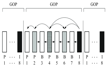
Figure 3: A closed GOP with $4$ layers and $8$ frames (a sequence of I, P and B frames).

VIII-B Simulation Results

We present the simulation results comparing the performance of our proposed EW-IDNC and NOW-IDNC algorithms to the following algorithms.

• Expanding window RLNC (EW-RLNC) algorithm [16, 18] that uses RLNC strategies to encode the packets in different windows while taking into account the decoding order of video layers and the hard deadline. The encoding and decoding processes of EW-RLNC algorithm are described in Appendix A.

• Maximum clique (Max-Clique) algorithm [23] that uses IDNC strategies to service a large number of receivers with any new packet in each transmission while ignoring the decoding order of video layers and the hard deadline.

• Interrelated priority encoding (IPE) algorithm [28] that uses IDNC strategies to reduce the number of transmissions required for delivering the base layer packets while ignoring the hard deadline.

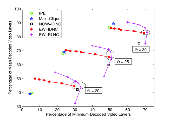
Figure 4: Percentage of mean decoded video layers versus percentage of minimum decoded video layers for different deadlines $\Theta$

Figs. 4 and 5 show the percentage of mean decoded video layers and the percentage of minimum decoded video layers performances of different algorithms for different deadlines $\Theta$ (for $M=15,\epsilon=0.2$) and different numbers of receivers $M$ (for $\Theta=25,\epsilon=0.2$). We choose 6 values for threshold $\lambda$ from [0.2, 0.95] with step size of 0.15. This results in 6 points on each trade-off curve of EW-IDNC and EW-RLNC algorithms such as $\lambda=0.2$ and $\lambda=0.95$ correspond to the top point and the bottom point, respectively. Moreover, we use ellipses to represent efficient operating points (i.e., thresholds $\lambda$) on the trade-off curves. From both figures, we can draw the following observations:

• As expected from EW-IDNC and EW-RLNC algorithms, the minimum decoded video layers over all receivers increases with the increase of threshold $\lambda$ at the expense of reducing the mean decoded video layers over all receivers. In general, given a small threshold $\lambda$, the design criterion is satisfied for a large number of video layers in each transmission, which results in a large coding window and a low level of protection to the lower video layers. Consequently, several receivers may decode a large number of video layers, while other receivers may decode only the first video layer before the deadline. To increase the minimum decoded video layers while respecting the mean decoded video layers, an efficient threshold $\lambda$ for the EW-IDNC algorithm is around $0.95$ and an efficient threshold $\lambda$ for the EW-RLNC algorithm is around $0.65$.

• EW-RLNC algorithm performs poorly for large thresholds (e.g., $\lambda=0.95$ representing the bottom point on the trade-off curve) due to transmitting a large number of coded packets from the smaller windows to obtain high decoding probabilities of the lower video layers at all receivers. Note that EW-RLNC algorithm explicitly determines the number of coded packets from each window at the beginning of the $\Theta$ transmissions. In contrast, our proposed EW-IDNC algorithm uses feedbacks to determine an efficient coding window in each transmission.

  

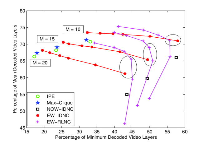
  Figure 5: Percentage of mean decoded video layers versus percentage of minimum decoded video layers for different number of receivers $M$

• Our proposed EW-IDNC algorithm achieves similar performances compared to the EW-RLNC algorithm in terms of the minimum and the mean decoded video layers. In fact, both algorithms guarantee a high probability of completing the broadcast of a lower video layer (using threshold $\lambda$) before expanding the window over the successor video layers.

• Our proposed NOW-IDNC algorithm achieves a similar performance compared to EW-IDNC and EW-RLNC algorithms in terms of the minimum decoded video layers. However, the NOW-IDNC algorithm performs poorly in terms of the mean decoded video layers due to always selecting a packet combination over a single video layer.

  

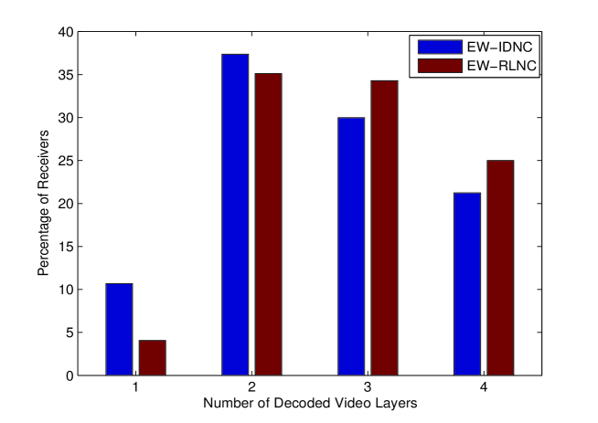
  Figure 6: Histogram showing the percentage of receivers that successfully decode one, two, three and four video layers before the deadline

• As expected, Max-Clique and IPE algorithms perform poorly compared to our proposed EW-IDNC and NOW-IDNC algorithms in terms of the minimum decoded video layers. Both Max-Clique and IPE algorithms make coding decisions across all video layers and thus, do not address the hard deadline for the most important video layer. As a result, several receivers may receive packets from the higher video layers, which cannot be used for decoding those video layers if a packet in a lower video layer is missing after the deadline.

Fig. 6 shows the histogram obtained by EW-IDNC algorithm (using $\lambda=0.95$) and EW-RLNC algorithm (using $\lambda=0.65$) for $\Theta=25,M=15,\epsilon=0.2$. This histogram illustrates the percentage of receivers that successfully decode one, two, three and four video layers before the deadline. From this histogram, we can see that most of the receivers decode three or four video layers out of four video layers in a GOP. Moreover, the percentage of receivers that decode the first four video layers in EW-RLNC algorithm is slightly higher compared to that in EW-IDNC algorithm. This better performance of EW-RLNC algorithm comes at the expense of higher packet overhead, higher encoding and decoding complexities as discussed in Section I.

IX Conclusion

In this paper, we developed an efficient, yet computationally simple, IDNC framework for real-time scalable video broadcast over wireless networks. In particular, we derived an upper bound on the probability that the individual completion times of all receivers meet the deadline. Using this probability with other guidelines, we designed EW-IDNC and NOW-IDNC algorithms that provide a high level of protection to the most important video layer before considering additional video layers in coding decisions. We used a real scalable video stream in the simulation and showed that our proposed IDNC algorithms improve the received video quality compared to the existing IDNC algorithms and achieve a similar performance compared to the EW-RLNC algorithm. Future research direction is to extend the proposed IDNC framework to cooperative systems, where the receivers cooperate with each other to recover their missing packets [33]. In general, the short-range channels between the receivers are better compared to the long-range channels between the base station to the receivers, which can be beneficial for real-time video streams with hard deadlines.

Appendix A Expanding Window Random Linear Network Coding

We follow the work in [18] and consider a deterministic approach, where the number of coded packets from each window is explicitly determined at the beginning of the period of $\Theta$ transmissions. The sender broadcasts these coded packets in $\Theta$ transmissions without receiving any feedback. Let us assume that $\theta_{\ell}$ coded packets are generated (and thus transmitted) from the packets in the $\ell$-th window $\omega_{\ell}$. Then $\Sigma_{\ell=1}^{L}\theta_{\ell}=\Theta$ and $\mathbf{z}=[\theta_{1},\theta_{2},...,\theta_{L}]$ is an EW-RLNC transmission policy. Given a fixed number of allowable transmissions $\Theta$, all possible transmission policies can be defined as all combinations of the number of coded packets from each window. Now, we describe the process of selecting a transmission policy as follows.

We use $\mathbf{n}=[n_{1},n_{2},...,n_{L}]$ to denote the number of packets from different layers in a GOP. For a given transmission policy $\mathbf{z}$, we denote the probability that receiver $R_{i}$ with erasure probability $\epsilon_{i}$ can decode the packets of layer $\ell$ (and all the packets of its lower layers) by $\mathds{P}_{i}^{\ell}(\mathbf{n},\mathbf{z})$. This probability can be computed using expression (1) in [18]. Now we extend this probability to $M$ receivers and compute the probability that $M$ receivers can decode the packets of layer $\ell$ (and all the packets of its lower layers) as follows:

$$\mathds{P}^{\ell}(\mathbf{n},\mathbf{z})=\prod_{R_{i}\in\mathcal{M}}\mathds{P}_{i}^{\ell}(\mathbf{n},\mathbf{z}).$$ (23)

Given transmission policy $\mathbf{z}$, the probability in (23) is computed for each of $L$ video layers. Furthermore, we consider all possible transmission policies and compute probability $\mathds{P}^{\ell}(\mathbf{n},\mathbf{z}),\forall\ell\in[1,...,L]$, for each transmission policy. Finally, we select the transmission policy $\mathbf{z}$ among all transmission policies that satisfies condition $\mathds{P}^{\ell}(\mathbf{n},\mathbf{z})\geq\lambda$ for the largest number of $\ell$ successive video layers (i.e., satisfies condition for the largest $\ell$-th video layer and of course all its lower layers). Here, condition $\mathds{P}^{\ell}(\mathbf{n},\mathbf{z})\geq\lambda$ is adopted following the same approach as in our proposed EW-IDNC algorithm. The details of decoding a video layer based on the number of received packets from different windows can be found in [18].

References

- [1] S. Katti, H. Rahul, W. Hu, D. Katabi, M. Médard, and J. Crowcroft, “Xors in the air: practical wireless network coding,” in ACM SIGCOMM Comput. Commun. Review, vol. 36, no. 4, 2006, pp. 243–254.
- [2] W. Zeng, C. T. Ng, and M. Médard, “Joint coding and scheduling optimization in wireless systems with varying delay sensitivities,” in 9th Annual IEEE Communications Society Conference on Sensor, Mesh and Ad Hoc Communications and Networks (SECON), 2012, pp. 416–424.
- [3] X. Wang, C. Yuen, and Y. Xu, “Coding-based data broadcasting for time-critical applications with rate adaptation,” IEEE Trans. Veh. Technol., vol. 63, no. 5, pp. 2429–2442, 2014.
- [4] M. Muhammad, M. Berioli, and T. de Cola, “A simulation study of network-coding-enhanced pep for tcp flows in geo satellite networks,” in IEEE International Conference on Communications (ICC), 2014, pp. 3588–3593.
- [5] Z. Dong, X. Wang, S. H. Dau, and C. Yuen, “Delay minimization for relay-based cooperative data exchange with network coding,” in IEEE 78th Vehicular Technology Conference (VTC Fall), 2013, pp. 1–5.
- [6] M. Yan and A. Sprintson, “Weakly secure network coding for wireless cooperative data exchange,” in IEEE Global Telecommunications Conference (GLOBECOM), 2011, pp. 1–5.
- [7] J. El-Najjar, H. M. AlAzemi, and C. Assi, “On the interplay between spatial reuse and network coding in wireless networks,” IEEE Trans. Wireless Commun., vol. 10, no. 2, pp. 560–569, 2011.
- [8] X. Li, C.-C. Wang, and X. Lin, “On the capacity of immediately-decodable coding schemes for wireless stored-video broadcast with hard deadline constraints,” IEEE J. Sel. Areas Commun., vol. 29, no. 5, pp. 1094–1105, 2011.
- [9] ——, “Optimal immediately-decodable inter-session network coding (idnc) schemes for two unicast sessions with hard deadline constraints,” in 49th Annual Allerton Conference on Communication, Control, and Computing (Allerton), 2011, pp. 784–791.
- [10] E. Magli, M. Wang, P. Frossard, and A. Markopoulou, “Network coding meets multimedia: A review,” IEEE Trans. Multimedia, vol. 15, no. 5, pp. 1195–1212, 2013.
- [11] H. Seferoglu and A. Markopoulou, “Video-aware opportunistic network coding over wireless networks,” IEEE J. Sel. Areas Commun., vol. 27, no. 5, pp. 713–728, 2009.
- [12] H. Seferoglu, L. Keller, B. Cici, A. Le, and A. Markopoulou, “Cooperative video streaming on smartphones,” in 49th Annual Allerton Conference on Communication, Control, and Computing (Allerton), 2011, pp. 220–227.
- [13] S. Y. El Rouayheb, M. A. R. Chaudhry, and A. Sprintson, “On the minimum number of transmissions in single-hop wireless coding networks,” in IEEE Information Theory Workshop (ITW), 2007, pp. 120–125.
- [14] P. Seeling, M. Reisslein, and B. Kulapala, “Network performance evaluation using frame size and quality traces of single-layer and two-layer video: A tutorial,” IEEE Commun. Surveys Tuts., vol. 6, no. 3, pp. 58–78, 2004.
- [15] H. Schwarz, D. Marpe, and T. Wiegand, “Overview of the scalable video coding extension of the h. 264/avc standard,” IEEE Trans. Circuits Syst. Video Technol., vol. 17, no. 9, pp. 1103–1120, 2007.
- [16] D. Vukobratovic and V. Stankovic, “Unequal error protection random linear coding strategies for erasure channels,” IEEE Trans. Commun., vol. 60, no. 5, pp. 1243–1252, 2012.
- [17] S. Wang, C. Gong, X. Wang, and M. Liang, “An efficient retransmission strategy for wireless scalable video multicast,” IEEE Wireless Commun. Lett., vol. 1, no. 6, pp. 581–584, 2012.
- [18] M. Esmaeilzadeh, P. Sadeghi, and N. Aboutorab, “Random linear network coding for wireless layered video broadcast: General design methods for adaptive feedback-free transmission,” 2014. [Online]. Available: http://arxiv.org/abs/1411.1841
- [19] L. Lima, S. Gheorghiu, J. Barros, M. Médard, and A. L. Toledo, “Secure network coding for multi-resolution wireless video streaming,” IEEE J. Sel. Areas Commun., vol. 28, no. 3, pp. 377–388, 2010.
- [20] P. Sadeghi, R. Shams, and D. Traskov, “An optimal adaptive network coding scheme for minimizing decoding delay in broadcast erasure channels,” EURASIP J. on Wireless Commun. and Netw., pp. 1–14, 2010.
- [21] S. Sorour and S. Valaee, “Minimum broadcast decoding delay for generalized instantly decodable network coding,” in IEEE Global Telecommunications Conference (GLOBECOM), 2010, pp. 1–5.
- [22] L. Keller, E. Drinea, and C. Fragouli, “Online broadcasting with network coding,” in Fourth Workshop on Network Coding, Theory, and Applications (NetCod), 2008, pp. 1–6.
- [23] A. Le, A. S. Tehrani, A. G. Dimakis, and A. Markopoulou, “Instantly decodable network codes for real-time applications,” in International Symposium on Network Coding (NetCod), 2013, pp. 1–6.
- [24] S. Sorour and S. Valaee, “On minimizing broadcast completion delay for instantly decodable network coding,” in IEEE International Conference on Communications (ICC), 2010, pp. 1–5.
- [25] N. Aboutorab, P. Sadeghi, and S. Sorour, “Enabling a tradeoff between completion time and decoding delay in instantly decodable network coded systems,” IEEE Trans. Commun., vol. 62, no. 4, pp. 1296 –1309, 2014.
- [26] C. Zhan, V. C. Lee, J. Wang, and Y. Xu, “Coding-based data broadcast scheduling in on-demand broadcast,” IEEE Trans. Wireless Commun., vol. 10, no. 11, pp. 3774–3783, 2011.
- [27] M. Muhammad, M. Berioli, G. Liva, and G. Giambene, “Instantly decodable network coding protocols with unequal error protection,” in IEEE International Conference on Communications (ICC), 2013, pp. 5120–5125.
- [28] S. Wang, C. Gong, X. Wang, and M. Liang, “Instantly decodable network coding schemes for in-order progressive retransmission,” IEEE Commun. Lett., vol. 17, no. 6, pp. 1069–1072, 2013.
- [29] M. R. Garey and D. S. Johnson, Computers and intractability. freeman New York, 1979.
- [30] J. Hastad, “Clique is hard to approximate within n 1-&epsiv,” in IEEE 37th Annual Symposium on Foundations of Computer Science, 1996, pp. 627–636.
- [31] “Test video sequences (retrieved june 2014).” [Online]. Available: ftp://ftp.tnt.uni-hannover.de/pub/svc/testsequences/
- [32] “Joint scalable video model (jsvm) reference software, version 9.19.14,” 2011. [Online]. Available: http://www.hhi.fraunhofer.de/en/fields-of-competence/image-processing/research-groups/image-video-coding/svc-extension-of-h264avc/jsvm-reference-software.html
- [33] N. J. Hernandez Marcano, J. Heide, D. E. Lucani, and F. H. Fitzek, “On the throughput and energy benefits of network coded cooperation,” in IEEE 3rd International Conference on Cloud Networking (CloudNet), 2014, pp. 138–142.