Possible Evidence for Planck-Scale Resonant Particle Production during Inflation from the CMB Power Spectrum

Abstract

The power spectrum of the cosmic microwave background from both the Planck and WMAP data exhibits a slight dip for multipoles in the range of $l=10-30$. We show that such a dip could be the result of the resonant creation of massive particles that couple to the inflaton field. For our best-fit models, the epoch of resonant particle creation reenters the horizon at a wave number of $k_{*}\sim 0.00011\pm 0.0004$ ($h$ Mpc^-1). The amplitude and location of this feature corresponds to the creation of a number of degenerate fermion species of mass $\sim(8-11)/\lambda^{3/2}$ $m_{pl}$ during inflation where $\lambda\sim(1.0\pm 0.5)N^{-2/5}$ is the coupling constant between the inflaton field and the created fermion species, while $N$ is the number of degenerate species. Although the evidence is of marginal statistical significance, this could constitute new observational hints of unexplored physics beyond the Planck scale.

I INTRODUCTION

The Planck Satellite PlanckXIII ; PlanckXX has provided the highest resolution yet available in the determination of the power spectrum of the cosmic microwave background (CMB). Analysis of this power spectrum provides powerful constraints on the physics of the very early universe PlanckXX .

The primordial power spectrum is believed to derive from quantum fluctuations generated during the inflationary epoch Liddle ; cmbinflate . In this paper we discuss a peculiar feature visible in the observed power spectrum near multipoles $\ell=10-30$. This is an interesting region in the CMB power spectrum because it corresponds to angular scales that are not yet in causal contact, so that the observed power spectrum is close to the true primordial power spectrum.

An illustration of the Planck observed power spectrum in this region is shown in Figure 1. Although the error bars are large, there is a noticeable systematic deviation in the range $\ell=10-30$ below the best fit based upon the standard $\Lambda$CDM cosmology with a power-law primordial power spectrum. There is also a well-known possible suppression of the quadrupole moment in the CMB (not shown). These same features are visible in the CMB power spectrum from the Wilkinson Microwave Anisotropy Probe (WMAP) WMAP9 , and hence, are likely a true feature in the CMB power spectrum, although it should be noted that in the Planck Cosmological Parameters paper PlanckXX the deviation from a simple power law in the range $\ell=10-30$ was deduced to be of weak statistical significance due to the large cosmic variance at low $\ell$.

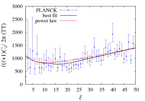
Figure 1: (Color online) CMB power spectrum in the range of $\ell=3-50$ Points with error bars are from the Planck Data Release PlanckXIII . The dashed line shows the best standard $\Lambda$CDM fit to the Planck CMB power spectrum based upon a power-law primordial power spectrum. The solid line shows the best fit for a model with resonant particle creation during inflation.

Nevertheless, a number of mechanisms have been proposed Iqbal15 to deal with the suppression of the power spectrum on large scales and low multipoles. In addition to being an artifact of cosmic variance PlanckXX ; Efstathiou03a , large-scale power suppression could arise from changes in the effective inflation-generating potential Hazra14 , differing initial conditions at the beginning of inflation Berera98 ; Contaldi03 ; Boyanovsky06 ; Powell07 ; Wang08 ; Broy15 ; Cicoli14 ; Das15 ; Mathews15 , the ISW effect Das14b , effects of spatial curvature Efstathiou03b , non-trivial topology Luminet03 , geometry Campanelli06 ; Campanelli07 , a violation of statistical anisotropies Hajian03 , effects of a cosmological-constant type of dark energy during inflation Gordon04 , the bounce due to a contracting phase to inflation Piao04 ; Liu13 , the production of primordial micro black-holes Scardigli11 , hemispherical anisotropy and non-gaussianity McDonald14a ; McDonald14b , the scattering of the inflationary trajectory in multiple field inflation by a hidden feature in the isocurvature direction Wang15 , brane symmetry breaking in string theory Kitazawa14 ; Kitazawa15 , quantum entanglement in the M-theory landscape Holman08 , or loop quantum cosmology Barrau14 , etc. Most of these works, however, were mainly concerned with the suppression of the lowest moments.

In the present work, however, we are concerned specifically with suppression of the power spectrum in the range $\ell=10-30$. In spite of the weak statistical significance, several recent works PlanckXX ; Hazra14 ; Kitazawa14 ; Kitazawa15 ; Wang15 have deemed it worthwhile to consider the physical consequences of this deviation, as it could point the way to new interesting physics at and above the Planck scale.

Indeed, in the Planck cosmological analysis PlanckXX the inflaton potential and the Hubble parameter evolution were reconstructed during the observable part of inflation by using a Taylor expansion of the inflaton potential or $H(\phi)$. When higher-order terms were allowed, both reconstructions found a change in the slope of the potential at the beginning of the observable range, thus better fitting the low-$\ell$ temperature deficit. As noted in that paper, however, these models were not significantly favored compared to lower order parameterizations that lead to slow-roll evolution at all times.

Also, in the Planck analysis three distinct methods to reconstruct the primordial power spectrum all independently found common patterns in the primordial power spectrum of curvature perturbations related to the dip at $\ell=10-30$ in the temperature power spectrum.

Although it is of weak statistical significance, a number of works have proposed explanations of this particular dip anomaly as a possible hint of new physics. One way to explain the anomaly is by a phase transition in the inflation potential Hazra14 . This is consistent with the abrupt changes in the slope of the inflation potential noted in the Planck reconstruction PlanckXX .

In Ref. Hazra14 this feature was fit with a class of models dubbed first order Wiggly Whipped inflation whereby the field starts rolling from a steeper power law potential and smoothly transitions to a flat power law potential. This sharp feature in the inflaton potential produces a departure from the initial slow-roll phase, imprinting a large scale suppression in the scalar primordial power spectrum. The best fits to the dip in such large field models were found to have a transition from a faster roll to the slow roll inflation at an inflaton field value of $\phi\approx 15~{}m_{pl}$.

As noted in that paper, however, in general this transition and any features in the large field potential produce a suppression of scalar relative to tensor modes at small $k$. This, however, is not consistent with the latest Planck results PlanckXX indicating a small tensor to scalar ratio. This fit also introduces wiggles in the primordial perturbation. Such wiggles in the matter power spectrum might also be used to constrain this possibility.

In Kitazawa14 ; Kitazawa15 the suppression of low multipoles and the dip for $\ell=10-30$ were simultaneously fit in a string-theory brane symmetry breaking mechanism. This mechanism splits boson and fermion excitations in string theory, leaving behind an exponential potential that is too steep for the inflaton to emerge from the initial singularity while descending it. As a result, the scalar field generically ”bounces against an exponential wall.” Just as in Hazra14 , this steep potential then introduces an infrared depression and a pre inflationary break in the power spectrum of scalar perturbations, reproducing the observed feature.

In Wang15 the dip at $\ell=10-30$ is explicitly related to the CMB cold spot with an angular radius of $\sim 10^{o}$ noted in both the Planck PlanckXIII and the WMAP WMAP9 sky maps in the direction $(l,b)=(209^{o},-57^{o})$. In their scenario, this could be due to a scattering of a multiple-field inflationary trajectory off of a hidden feature in the isocurvature direction. The inflaton then loses some energy. If only a patch of the sky hits that feature due to stochastic fluctuations then a cold spot in the sky and a corresponding dip in the temperature power spectrum ensues.

In the present work, however, rather than to address the implications for the inflation-generating potential, we consider the possibility that new trans-Planckian physics occurs near the end of the inflation epoch corresponding to the resonant creation chung00 ; Mathews04 of Planck-scale particles that couple to the inflaton field. Our best fit is shown by the solid line in Figure 1 which we describe in detail in the following sections.

This interpretation has the intriguing aspect that, if correct, an opportunity emerges to use the CMB to probe properties of new particle species that existed at and above the Planck scale ($m_{pl}\sim 10^{19}$ GeV). That is the goal of the present work.

Indeed, massive particles generically exist at and above the Planck scale due to the compactification schemes of string theory from the Kaluza-Klein states, winding modes, string excitations, etc. Moreover, the coupling of the inflaton to other particle species near the end of inflation is not only natural, but probably required. This is because the energy density in the inflaton must be converted to entropy in light or heavy particle species at the end of inflation as a means to reheat the universe. Hence, the existence of Planck-scale mass particles that couple to the inflaton near the end of inflation is a scenario that is both natural and even required. Moreover, this provides a possible opportunity to uncover new physics in the trans-Planckian regime.

In our previous study Mathews04 a similar analysis was made of a possible bump in the CMB in the range of very high multipoles. At that time there appeared to be an excess power in the CMB power spectrum for multipoles in the range $\ell=2000-3500$ in the combined (CBI cbi1 ; cbi2 ; cbi3 , ACBAR acbar , BIMA BIMA , and VSA VSA ) data, contrary to the expectation from the WMAP results WMAP1 . Since that time, however, better high resolution data have eliminated the apparent excess.

The present analysis, however, is significantly different from that previous work. In place of a bump we now seek to fit a dip in the power spectrum. This is achieved by use of a different Lagrangian. Also, the feature we fit here is at low multipoles and therefore much more likely a part of the primordial spectrum. Moreover, the deduced particle properties are much different than that of the previous study and even of opposite sign coupling. Hence, here we present new results on possible resonant fermion particle production during inflation.

II Resonant Particle Production during Inflation

The details of the resonant particle creation paradigm during inflation have been explained in Refs. chung00 ; Mathews04 . Indeed, the idea was originally introduced Kofman94 as a means for reheating after inflation. Since chung00 subsequent work Elgaroy03 ; Romano08 ; Barnaby09 ; Fedderke15 has elaborated on the basic scheme into a model with coupling between two scalar fields. Here, we summarize essential features of the canonical single fermion field coupled to the inflaton as a means to clarify the possible physics of the $\ell=10-30$ dip.

In this minimal extension from the basic picture, the inflaton $\phi$ is postulated to couple to particles whose mass is of order the inflaton field value. These particles are then resonantly produced as the field obtains a critical value during inflation. If even a small fraction of the inflaton field is affected in this way, it can produce an observable feature in the primordial power spectrum. In particular, there can be either an excess in the power spectrum as noted in chung00 ; Mathews04 , or a dip in the power spectrum as described in this paper. Such a dip offers important new clues to the trans-Planckian physics of the early universe.

We note that particle creation corresponding to an imaginary part of the effective action of quantum fields has been considered in Starobinsky02 . In that case the same creation should occur at the present time. Thus, compatibility with the diffuse $\gamma$-ray background can be used to rule out the possibility of measurable effects from this type of trans-Planckian particle creation in the CMB anisotropy. However, the effect of interest here is a perturbation in the simple scalar field due to direct coupling to Planck-mass particles at energies for which the inflation potential is comparable to the particle mass and cannot occur at the present time. The present scenario, therefore is not constrained by the diffuse gamma-ray background.

In the simplest slow roll approximation Liddle ; cmbinflate , the generation of density perturbations of amplitude, $\delta_{H}(k)$, when crossing the Hubble radius is just,

$$\delta_{H}(k)\approx{H^{2}\over 5\pi\dot{\phi}}~{}~{},$$ (1)

where $H$ is the expansion rate, and $\dot{\phi}$ is the rate of change of the inflaton field when the comoving wave number $k$ crosses the Hubble radius during inflation. We caution, however, that resonant particle production could affect the inflaton field. In that case the conjugate momentum in the field $\dot{\phi}$ could be altered. This could cause either an increase or a diminution in $\delta_{H}(k)$ (the primordial power spectrum) for those wave numbers which exit the horizon during the resonant particle production epoch. In particular, when $\dot{\phi}$ is accelerated due to particle production, it may deviate from the slow-roll condition. In chung00 , however, this correction was analyzed and found to be $<<20\%$. Hence, for our purposes we can ignore this correction.

For the application here, we adopt a positive Yukawa coupling of strength $\lambda$ between the inflaton field $\phi$ and the field $\psi$ of $N$ fermion species. This differs from chung00 ; Mathews04 who adopted a negative Yukawa coupling. With our choice, the total Lagrangian density including the inflaton scalar field $\phi$, the Dirac fermion field, and the Yukawa coupling term is then simply,

$${\cal L}_{\rm tot} = \frac{1}{2}\partial_{\mu}\phi\partial^{\mu}\phi-V(\phi)$$ (2)

$$+ i\bar{\psi}\not{\partial}\psi-m\bar{\psi}\psi+N\lambda\phi\bar{\psi}\psi~{}~{}.$$

For this Lagrangian, it is obvious that the fermions have an effective mass of

$$M(\phi)=m-N\lambda\phi~{}~{}.$$ (3)

This vanishes for a critical value of the inflaton field, $\phi_{*}=m/N\lambda$. Resonant fermion production will then occur in a narrow range of the inflaton field amplitude around $\phi=\phi_{*}$.

Note, that the vanishing of the effective mass term with a negative coupling term as in chung00 ; Mathews04 requires a positive mass term in the associated free particle Lagrangian. To achieve this a scenario was adopted in that paper whereby the inflaton $\phi$ controls the fermion mass $\psi$ through the coupling

$$L_{int}=-[M_{f}-M_{pl}f(\frac{\phi}{M_{pl}})]\bar{\psi}\psi~{}~{},$$ (4)

where $M_{f}$ is the fermion mass. In that case, imposing $f>>1$ leads to a positive mass term and a cancellation of the effective mass is possible. Here, however, we consider the simpler case of $f<<1$ so that a simple free-particle Lagrangian is sufficient.

As in chung00 ; Mathews04 we label the epoch at which particles are created by an asterisk. So, the cosmic scale factor is labeled $a_{*}$ at the time $t_{*}$ at which resonant particle production occurs. Considering a small interval around this epoch, one can treat $H=H_{*}$ as approximately constant (slow roll inflation). The number density $n$ of particles can be taken as zero before $t_{*}$ and afterwards as $n=n_{*}[a_{*}/a(t)]^{3}$. The fermion vacuum expectation value can then be written,

$$\langle\bar{\psi}\psi\rangle=n_{*}\Theta(t-t_{*})\exp{[-3H_{*}(t-t_{*})]}~{}~{}.$$ (5)

where $\Theta$ is a step function.

Then following the derivation in chung00 ; Mathews04 , we have the following modified equation of motion for the scalar field coupled to $\psi$:

$$\ddot{\phi}+3H\dot{\phi}=-V^{\prime}(\phi)+N\lambda\langle\bar{\psi}\psi\rangle~{}~{},$$ (6)

where $V^{\prime}(\phi)=dV/{d\phi}$. The solution to this differential equation after particle creation $(t>t_{*})$ is then similar to that derived in Refs. chung00 ; Mathews04 but with a sign change for the coupling term, i.e.

$$\dot{\phi}(t>t_{*}) = \dot{\phi}_{*}\exp{[-3H(t-t_{*})]}$$ (7)

$$- \frac{V^{\prime}(\phi)_{*}}{3H_{*}}\bigl{[}1-\exp{[-3H(t-t_{*})]}\bigr{]}$$

$$+ N\lambda n_{*}(t-t_{*})\exp{[-3H_{*}(t-t_{*})]}~{}~{}.$$

The physical interpretation here is that the rate of change of the scalar field rapidly increases due to the coupling to particles created at the resonance $\phi=\phi_{*}$.

Then, using Eq. (1) for the fluctuation as it exits the horizon, and constant $H\approx H_{*}$ in the slow-roll condition along with

$$d\ln{a}=Hdt~{}~{},$$ (8)

one obtains the perturbation in the primordial power spectrum as it exits the horizon:

$$\delta_{H}=\frac{[\delta_{H}(a)]_{N\lambda=0}}{1+\Theta(a-a_{*})(N\lambda n_{*}/|\dot{\phi}_{*}|H_{*})(a_{*}/a)^{3}\ln{(a/a_{*})}}~{}~{}.$$ (9)

Here, it is clear that the power in the fluctuation of the inflaton field will diminish as the particles are resonantly created when the universe grows to some critical scale factor $a_{*}$.

Using $k_{*}/k=a_{*}/a$, then the perturbation spectrum Eq. (9) can be reduced Mathews04 to a simple two-parameter function.

$$\delta_{H}(k)=\frac{[\delta_{H}(a)]_{N\lambda=0}}{1+\Theta(k-k_{*})A(k_{*}/k)^{3}\ln{(k/k_{*})}}~{}~{}.$$ (10)

where the amplitude $A$ and characteristic wave number $k_{*}$ ($k/k_{*}\geq 1$) can be fit to the observed power spectrum from the relation:

$$k_{*}=\frac{\ell_{*}}{r_{lss}}~{}~{},$$ (11)

where $r_{lss}$ is the comoving distance to the last scattering surface, taken here to be 14 Gpc.

The connection between resonant particle creation and the CMB temperature fluctuations is straightforward. As usual, temperature fluctuations are expanded in spherical harmonics, $\delta T/T=\sum_{l}\sum_{m}a_{lm}Y_{lm}(\theta,\phi)$ ($2\leq l<\infty$ and $-l\leq m\leq l$). The anisotropies are then described by the angular power spectrum, $C_{l}=\langle|a_{lm}|^{2}\rangle$, as a function of multipole number $l$. One then merely requires the conversion from perturbation spectrum $\delta_{H}(k)$ to angular power spectrum $C_{l}$. This is easily accomplished using the CAMB code Camb . When converting to the angular power spectrum, the amplitude of the narrow particle creation feature in $\delta_{H}(k)$ is spread over many values of $\ell$. Hence, the particle creation feature looks like a broad dip in the power spectrum.

We have made a multi-dimensional Markov Chain Monte-Carlo analysis Christensen ; Lewis of the CMB using the Planck data PlanckXIII and the CosmoMC code Lewis . For simplicity and speed in the present study we only marginalized over parameters which do not alter the matter or CMB transfer functions. Hence, we only varied $A$ and $k_{*}$, along with the six parameters, $\Omega_{b}h^{2},\Omega_{c}h^{2},\theta,\tau,n_{s},A_{s}$. Here, $\Omega_{b}$ is the baryon content, $\Omega_{c}$ is the cold dark matter content, $\theta$ is the acoustic peak angular scale, $\tau$ is the optical depth, $n_{s}$ is the power-law spectral index, and $A_{s}$ is the normalization. As usual, both $n_{s}$ and $A_{s}$ are normalized at $k=0.05$ Mpc^-1.

Figure 2 shows contours of likelihood for the resonant particle creation parameters, $A$ and $k_{*}$. Adding this perturbation to the primordial power spectrum improves the total $\chi^{2}$ for the fit from 9803 to 9798. One expects that the effect of interest here would only make a small change ($\Delta\chi^{2}=5$) in the overall fit because it only affects a limited range of $l$ values with large error bars. Nevertheless, from the likelihood contours we can deduce a mean value of $A=1.7\pm 1.5$ with a maximum likelihood value of $A=1.5$, and a mean value of $k_{*}=0.0011\pm 0.0004~{}h~{}{\rm Mpc}^{-1}$

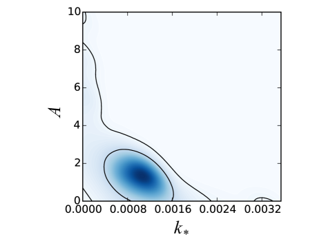
Figure 2: (Color online) Constraints on parameters $A$ and $k_{*}$ from the MCMC analysis of the CMB power spectrum. Contours show 1 and 2$\sigma$ limits. The horizontal axis is in units of ($h$ Mpc^-1).

Of course, it is obvious that adding extra parameters should improve the goodness of fit. One should quantify the statistical significance of the improvement over a simple power-law primordial power spectrum. A $\Delta\chi^{2}=5$ in the fit corresponds to a 92% confidence level for two free parameters, hence less than a 2$\sigma$ confidence limit. To be more precise, the Bayesian information criterion (BIC) can be used to select whether one model is better than another by introducing a penalty term for the number of parameters in the model fit. Under the assumption that the model errors are independent and obey a normal distribution, then the BIC can be rewritten in terms of $\Delta\chi^{2}$ as BIC$\approx\Delta\chi^{2}+df\cdot\ln{n}$ where $df$ is the number of degrees of freedom in the test and $n$ is the number of points in the observed data. For the 30 multipoles in the range of the fit, the introduction of 2 new free parameters then corresponds to a BIC$=1.8$. Generally, BIC$>2$ is considered positive evidence for an improvement in the fit. Hence, one must conclude that the evidence for this fit is statistically weak. Nevertheless, it is worthwhile to examine the possible physical meaning of the deduced parameters.

III Physical Parameters

The values of $A$ and $k_{*}$ determined from from the CMB power spectrum relate to the inflaton coupling $\lambda$ and fermion mass $m$, for a given inflation model via Eqs. (9) and (10).

$$A=|\dot{\phi}_{*}|^{-1}N\lambda n_{*}H_{*}^{-1}~{}~{}.$$ (12)

The coefficient $A$ can be related directly to the coupling constant $\lambda$ using the approximation chung00 ; birrellanddavies ; Kofman:1997yn ; Chung:1998bt for the particle production Bogoliubov coefficient

$$|\beta_{k}|^{2}=\exp\left(\frac{-\pi k^{2}}{a_{*}^{2}N\lambda|\dot{\phi}_{*}|}\right).$$ (13)

Then,

$$n_{*}=\frac{2}{\pi^{2}}\int_{0}^{\infty}dk_{p}\,k_{p}^{2}\,|\beta_{k}|^{2}=\frac{N\lambda^{3/2}}{2\pi^{3}}|\dot{\phi}_{*}|^{3/2}~{}~{}.$$ (14)

This give us

$$A = \frac{N\lambda^{5/2}}{2\pi^{3}}\frac{\sqrt{|\dot{\phi}_{*}|}}{H_{*}}$$ (15)

$$\approx \frac{N\lambda^{5/2}}{2\sqrt{5}\pi^{7/2}}\frac{1}{\sqrt{\delta_{H}(k_{*})|_{\lambda=0}}}~{}~{}.$$ (16)

where we have used the usual approximation for the primordial slow roll inflationary spectrum Liddle ; cmbinflate . This means that regardless of the exact nature of the inflationary scenario, for any fixed inflationary spectrum $\delta_{H}(k)|_{\lambda=0}$ without the back reaction, we have the particle production giving a dip of the form Eq. (10) with the parameter $A$ expressed in terms of the coupling constant through Eq. (16). Given that the CMB normalization requires $\delta_{H}(k)|_{\lambda=0}\sim 10^{-5}$, we then have

$$A\sim 1.3N\lambda^{5/2}.$$ (17)

Hence, for the maximum likelihood value of $A\sim 1.5$, we have

$$\lambda\approx\frac{(1.0\pm 0.5)}{N^{2/5}}~{}~{}.$$ (18)

So, $\lambda\leq 1$ requires $N>1$ as expected.

The fermion particle mass $m$ can then be deduced from $m=N\lambda\phi_{*}$. From Eq. (18) then we have $m\approx\phi_{*}/\lambda^{3/2}$. For this purpose, however, one must adopt a specific form for the inflaton potential to determine $\phi_{*}$ appropriate to the scale $k_{*}$. Here, we adopt a general monomial potential whereby:

$$V(\phi)=\Lambda_{\phi}m_{pl}^{4}\biggl{(}\frac{\phi}{m_{pl}}\biggr{)}^{\alpha}~{}~{},$$ (19)

for which there is a simple analytic relation Liddle between the value of $\phi_{*}$ and the number of e-folds ${\cal N}(k_{*})$ between when $k_{*}$ exits the horizon and the end of inflation, i.e.

$${\cal N}(k_{*})=\frac{1}{m_{\rm pl}^{2}}\int_{\phi_{end}}^{\phi_{*}}\frac{V(\phi)}{V^{\prime}(\phi)}d\phi~{}~{},$$ (20)

implies

$$\phi_{*}=\sqrt{2\alpha{\cal N}}m_{pl}~{}~{}.$$ (21)

For $k_{*}=0.0011\pm 0.0004~{}h~{}{\rm Mpc}^{-1}$, and $k_{H}=a_{0}H_{0}=(h/3000)$ Mpc${}^{-1}\sim 0.0002,$ we have ${\cal N}-{\cal N}_{*}=ln{(k_{H}/k_{*})}<1$. Typically one expects ${\cal N}(k_{*})\sim{\cal N}\sim 50-60$. We note, however, that one can have the number of e-folds as low as ${\cal N}\sim 25$ in the case of thermal inflation Liddle . For standard inflation a monomial potential with $\alpha=2$ would have $\phi_{*}\sim(14-15)~{}m_{pl}$. However, the limits on the tensor to scalar ration from the Planck analysis PlanckXX rule out $\alpha=2$ at the 95% confidence level. Monomial potentials are more consistent with $\alpha=1$ ($\phi_{*}=(10-11)~{}m_{pl}$), or even $\alpha=2/3$ ($\phi_{*}=(8-9)~{}m_{pl}$). Hence, we have roughly the constraint,

$$m\sim(8-11)~{}\frac{m_{\rm pl}}{\lambda^{3/2}}~{}~{}.$$ (22)

So, one can deduce a family of possible properties of the resonantly produced particle (i.e. its mass and coupling strength) in terms of a single parameter, the degeneracy $N$. This is illustrated in Figure 3 that shows allowed values and uncertainty in the coupling constant and particle mass as a function of the number of degenerate species for a $\phi^{2/3}$ inflaton effective potential experiencing 50 $e$-folds of inflation.

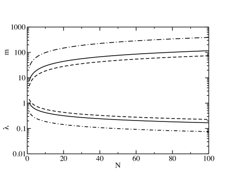
Figure 3: Implied values of $\lambda$ and $m$ as a function of the number of degenerate species $N$ for a $\phi^{2/3}$ inflaton effective potential experiencing 50 $e$-folds of inflation. Upper curves show the allowed mass. Lower curves are the coupling constant. Solid line is for the best-fit normalization $A=1.5$. The dashed and dot-dashed lines show the uncertainties due to the upper and lower limits on $A$, respectively.

Indeed, it is natural chung00 to have a large degeneracy (e.g. $N\sim 10-100$ in Figure 3) among trans-Planckian massive particles. Supergravity and super-string theories generally contain a spectrum of particles with masses well in excess of the Planck mass. Moreover, the compact extra-dimensions lead to a tower of nearly degenerate Kaluza-Klein (KK) states Kolb84 ; Lewis03 , and as noted above, reheating may require that some of these particles couple to the inflaton field near the end of inflation.

IV Matter Power Spectrum

It is perhaps obvious that the matter power spectrum will be unaffected by the $\ell=10-30$ anomaly since, as noted above, this range of multipoles is for the most part not yet in causal contact. Nevertheless, the largest multipoles affected by this dip are near the scale of the horizon at decoupling. Hence, as in other studies Hazra14 for completeness, we examine the impact of this anomaly on the matter power spectrum.

It is straight forward to determine the matter power spectrum. To convert the amplitude of the perturbation as each wave number $k$ enters the horizon, $\delta_{H}(k)$, to the present-day power spectrum, $P(k)$, which describes the amplitude of the fluctuation at a fixed time, one utilizes the transfer function, $T(k)$ efstathiou which is easily computed using the CAMB code Camb for various sets of cosmological parameters (e.g. $\Omega$, $H_{0}$, $\Lambda$, $\Omega_{B}$). An adequate approximate expression for the structure power spectrum is then

$$\frac{k^{3}}{2\pi^{2}}P(k)=\left(\frac{k}{aH_{0}}\right)^{4}T^{2}(k)\delta^{2}_{H}(k)\ .$$ (23)

This expression is only valid in the linear regime, which in comoving wave number is up to approximately $k^{<}_{\sim}0.2~{}h$ Mpc^-1 and therefore adequate for our purposes. However, we also correct for the nonlinear evolution of the power spectrum Peacock .

Figure 4 shows the matter power spectrum from the Wiggle-Z Dark Energy Survey wiggle compared to the computed maximum likelihood power spectrum with and without the perturbation due to the resonant particle creation. Unfortunately, the perturbation is on a scale too large to be probed by the observed matter power spectrum.

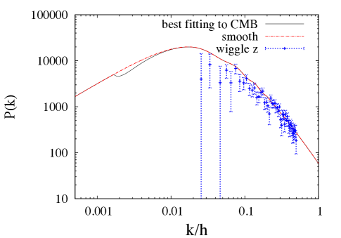
Figure 4: (Color online) Comparison of the observed galaxy cluster function from wiggle with the spectrum implied from the fits to the matter power spectrum with (solid line) and without (dashed line) resonant particle creation during inflation as described in the text.

V Conclusion

We have analyzed the $\ell=10-30$ dip in the Planck CMB power spectrum in the context of a model for the creation $N$ nearly degenerate trans-Planckian massive fermions during inflation. The best fit to the CMB power spectrum implies an optimum feature at $k_{*}=0.0011\pm 0.0004~{}h$ Mpc^-1 and $A\approx 1.7\pm 1.5$. For monomial inflation potentials consistent with the Planck tensor-to-scalar ratio, this feature would correspond to the resonant creation of nearly degenerate particles with $m\sim 8-11$ $m_{pl}/\lambda^{3/2}$ and a Yukawa coupling constant $\lambda$ between the fermion species and the inflaton field of $\lambda\approx(1.0\pm 0.5)N^{-2/5}$ for $N$ degenerate fermion species.

Obviously there is a need for more precise determinations of the CMB power spectrum for multipoles in the range of $\ell=10-30$, although this may ultimately be limited by the cosmic variance.

Nevertheless, in spite of these caveats, we conclude that if the present analysis is correct, this may be one of the first hints at observational evidence of new particle physics at the Planck scale. Indeed, one expects a plethora of particles at the Planck scale, particularly in the context of string theory. Perhaps, the presently observed CMB power spectrum contains the first suggestion that a subset of such particles may have coupled to the inflaton field leaving a relic signature of their existence in the CMB primordial power spectrum.

- (1) Planck Collaboration, Astron. & Astrophys. Submitted (2015) ArXive:1502.01589, astro-ph
- (2) Planck Collaboration, Astron. & Astrophys. Submitted (2015) ArXive:1502.02114, astro-ph
- (3) A. R. Liddle and D. H. Lyth, Cosmological Inflation and Large Scale Structure, (Cambridge University Press: Cambridge, UK), (1998).
- (4) E. W. Kolb and M. S. Turner, The Early Universe, (Addison-Wesley, Menlo Park, Ca., 1990).
- (5) G. Hinshaw, et al. (WMAP Collaboration) Astrophys. J. Suppl. Ser., 208, 19 (2013).
- (6) A. Iqbal, J. Prasad, T. Souradeep, and M. A. Malik, JCAP, 06, 014 (2015).
- (7) G. Efstathiou, Mon. Not. R. Astron. Soc. 346 L26, (2003).
- (8) D. K. Hazra, A. Shafieloo, G. F. Smoot, and A. A. Starobinsky, JCAP, 08, 048 (2014).
- (9) A. Berera, L.-Z. Fang, and G. Hinshaw, Phys. Rev. D 57 2207, (1998).
- (10) C. R. Contaldi, M. Peloso, L. Kofman, and A. Linde, JCAP 7 2, (2003).
- (11) D. Boyanovsky, H. J. de Vega, and N. G. Sanchez, Phys. Rev. D 74 123006, ( 2006).
- (12) B. A. Powell and W. H. Kinney, Phys. Rev. D 76 063512, (2007).
- (13) I.-Chin Wang and K.-W. Ng,Phys. Rev. D 77 083501, (2008).
- (14) B. J. Broy, D. Roest, and A. Westphal, Phys. Rev. D 91, 023514, (2015) .
- (15) M. Cicoli, S. Downes, B. Dutta, F. G. Pedro, and A. Westphal, JCAP 12 30, (2014).
- (16) S. Das, G. Goswami, J. Prasad, and R. Rangarajan, JCAP, 06, 01 (2015).
- (17) G. J. Mathews, I.-S. Suh, N. Q. Lan, and T. Kajino, Phys Rev. D, Submitted (2015).
- (18) S. Das and T. Souradeep, JCAP 2, 2, (2014).
- (19) G. Efstathiou, Mon. Not. R. Astron. Soc. 343 L95 (2003).
- (20) J.-P. Luminet, J. R. Weeks, A. Riazuelo, R. Lehoucq, and J.-P. Uzan, Nature, 425 593 (2003).
- (21) L. Campanelli, P. Cea, and L. Tedesco, Phys. Rev. Lett. 97 131302, (2006).
- (22) L. Campanelli, P. Cea, and L. Tedesco, Phys. Rev. D 76 063007, (2007).
- (23) A. Hajian and T. Souradeep, Astrophys. J. Lett. 597 L5, (2003).
- (24) C. Gordon and W. Hu, Phys. Rev. D 70 083003, (2004).
- (25) Y.-S. Piao, B. Feng, and X. Zhang, Phys. Rev. D 69 103520, (2004).
- (26) Z.-G. Liu, Z.-K. Guo, and Y.-S. Piao, Phys. Rev. D 88 063539, (2013).
- (27) F. Scardigli, C. Gruber, and P. Chen, Phys. Rev. D 83 063507 (2011).
- (28) J. McDonald, Phys. Rev. D 89 127303, (2014).
- (29) J. McDonald, JCAP 11 012, (2014).
- (30) Y. Wang and Y.-Z. Ma, eprint arXiv:1501.00282v1 (2015).
- (31) N. Kitazawa and A. Sagnotti, EPJ Web of Conferences 95, 03031 (2015).
- (32) N. Kitazawa and A. Sagnotti, Mod. Phys. Lett. A 30, 1550137 (2015).
- (33) R. Holman, L. Mersini-Houghton, and T. Takahashi, Phys. Rev. D 77, 063511 (2008).
- (34) A. Barrau, T. Cailleteau, J. Grain, and J. Mielczarek, Classical and Quantum Gravity 31 053001 (2014).
- (35) D. J. H. Chung, E. W. Kolb, A. Riotto, and I. I. Tkachev, Phys. Rev. D 62, 043508 (2000).
- (36) G. J. Mathews, D. Chung, K. Ichiki, T. Kajino, and M. Orito, Phys. Rev. D70, 083505 (2004).
- (37) B. S. Mason, et al. (CBI Collaboration), Astrophys. J., 591, 540 (2003).
- (38) T. J. Pearson, et al. (CBI Collaboration), Astrophys. J., 591, 556 (2003).
- (39) A. C. S. Readhead, et al., Astrophys. J. in press, (2004).
- (40) C. L. Kuo et al., (ACBAR Collaboration), Astrophys. J., 600, 32 (2004).
- (41) K. S. Dawson, et al., BIMA Collaboration), Astrophys. J., 581, 86 (2002).
- (42) K. Grainge, et al., VSA Collaboration), Mon. Not. R. Astron. Soc., 341, L23, (2003).
- (43) C. L. Bennett, et al. (WMAP Collaboration), Astrophys. J., Suppl., 148, 99 (2003); D. L. Spergel, et al., Astrophys. J. Suppl., 148, 175 (2003).
- (44) L. Kofman, A. D. Linde, and A. A. Starobinsky, Phys. Rev. Lett. 73 3195 (1994).
- (45) O. Elgaroy, S. Hannestad, and T. Haugboelle, JCAP, 09, 008 (2003).
- (46) A. E. Romano and M. Sasaki, Phys. Rev. D 78, 103522 (2008).
- (47) N. Barnaby, Z. Huang, L. Kofman, and D. Pogosyan, Phys. Rev. D 80, 043501 (2009).
- (48) M. A. Fedderke, E. W. Kolb, M. Wyman, Phys. Rev., D 91, 063505 (2015).
- (49) A. A. Starobinsky and I. I. Tkachev, J. Exp. Th. Phys. Lett., 76, 235 (2002).
- (50) A. Lewis, A. Challinor, and A. Lasenby, Astrophys. J., 538, 473 (2000).
- (51) N. Christensen and R. Meyer, L. Knox, and B. Luey, Class. and Quant. Grav., 18, 2677 (2001).
- (52) A. Lewis and S. Bridle, Phys. Rev. D 66, 103511 (2002).
- (53) N. D. Birrell and P. C. W. Davies, Quantum Fields in Curved Space, (Cambridge Univ. Press, Cambridge, 1982).
- (54) L. Kofman, A. Linde and A. A. Starobinsky, Phys. Rev. D 56, 3258 (1997).
- (55) D. J. H. Chung, Phys. Rev. D 67, 083514 (2003).
- (56) E. W. Kolb and R. Slansky, Phys. Lett 135B, 378 (1984).
- (57) Our Superstring Universe: Strings, Branes, Extra Dimensions and Superstring-M Theory , by L.E. Lewis, Jr. (iUniverse, Inc. NE, USA; 2003)
- (58) G. P. Efstathiou, in Physics of the Early Universe, (SUSSP Publications, Edinburgh, 1990), eds. A. T. Davies, A. Heavens, and J. Peacock.
- (59) J. A. Peacock and S. J. Dodds, Mon. Not. R. Astron. Soc., 280 L19 (1996).
- (60) E. A. Kazin, et al. (Wiggle-Z Dark Energy Survey), MNRAS 441, 3524 3542 (2014).